HypeR: Hypothetical Reasoning With What-If and How-To Queries Using a Probabilistic Causal Approach

Abstract.

What-if (provisioning for an update to a database) and how-to (how to modify the database to achieve a goal) analyses provide insights to users who wish to examine hypothetical scenarios without making actual changes to a database and thereby help plan strategies in their fields. Typically, such analyses are done by testing the effect of an update in the existing database on a specific view created by a query of interest. In real-world scenarios, however, an update to a particular part of the database may affect tuples and attributes in a completely different part due to implicit semantic dependencies. To allow for hypothetical reasoning while accommodating such dependencies, we develop HypeR, a framework that supports what-if and how-to queries accounting for probabilistic dependencies among attributes captured by a probabilistic causal model. We extend the SQL syntax to include the necessary operators for expressing these hypothetical queries, define their semantics, devise efficient algorithms and optimizations to compute their results using concepts from causality and probabilistic databases, and evaluate the effectiveness of our approach experimentally.

1. Introduction

Hypothetical reasoning is a crucial element in decision-making and risk assessment in business (GolfarelliR09a, ; singh2013use, ; ZhangCSW07, ), healthcare (Qureshi14, ; RamakrishnanNDSCE04, ), real estate (donner2018digital, ), etc. Such analysis is split by previous work into two categories: what-if analysis and how-to analysis. What-if analysis (BalminPP00, ; LakshmananRS08, ; HerodotouB11, ) is usually meant for testing assumptions and projections on a particular outcome by allowing users to pose queries about hypothetical updates in the database and examining their effect on a query result. Users detail a specific hypothetical scenario whose effect they wish to examine on their view of choice and the system computes the view as if the update has been performed in the database. On the other hand, how-to analysis (MeliouGS11, ; MeliouS12, ) has the reverse goal; users specify a target effect that they want to achieve and the system computes the appropriate hypothetical updates that have to be performed in the database to fulfill the goal.

Example 0.

Consider a simplified version of the Amazon product database (HeM16, ) shown in Figure 1 describing product details and product reviews. Each tuple has a unique tuple identifier next to it for clarity. Now, consider an analyst who wants to examine the effect of laptop prices on their Amazon ratings. She may ask “what would be the effect of increasing the price of Asus laptops by 10% on their average ratings?”. This what-if query asks about the effect of the hypothetical update on the database (increasing the Price) on a specific view (average Rating). She may also be interested in “what fraction of Asus laptops would have rating more than 4.0 if their price drops by $100?” or “What would be the average sentiment in the reviews for cameras if their color was changed to red?”. A different analyst may also be interested in maximizing the average rating of laptops reviews by changing their price. She may ask “how to maximize the average rating of laptops and cameras by updating the price of laptops so that it will not drop below 500 and increase above 800, and will be at most 100 away from it original value?” or “How to increase average sentiment in the reviews for cameras by changing their color?” Both queries are forms of hypothetical reasoning that can assist analysts and decision-makers in gaining insights about their products and their marketing strategies.

Multiple works in the database community have studied hypothetical reasoning. A substantial part of these (MeliouGS11, ; MeliouS12, ; DeutchIMT13, ; DeutchMT15, ; ArabG17, ; DeutchMR19, ) has focused on provenance updates and view manipulation as a main component for answering such queries. Therein, hypothetical updates are captured by changing values in the provenance and thus updating the view generated by the query of interest. However, in many real world situations, due to complex probabilistic causal dependencies between attributes of tuples that are relationally connected, updating an attribute of a tuple has collateral effects on other attributes of the same tuple, as well as attributes of other tuples. Such dependencies cannot be expressed and captured by provenance. We illustrate with an example.

Example 0.

Reconsider Example 1. The provenance of the average rating of Asus laptops will not change if the price of the laptops is augmented. Similarly, for the how-to query, the provenance of the average rating of laptops and cameras will not be affected by the change in price. Thus, previous work in databases fails to account for the collateral effect that increasing the price of a laptop may have on the user’s ratings. Note that due to our lack of knowledge about the underlying process that leads to the user’s ratings, we may only reason about the probabilistic effect of increasing the price on user’s ratings. Figure 2 gives an intuitive description of potential dependencies between the attributes of the database in Figure 1. For example, changing the Price of a laptop may affect its Rating (denoted as the edge from the blue Price node to the blue Rating node in Figure 2). Furthermore, increasing the Price of Asus laptops may affect the Rating of Vaio laptops and vice versa (denoted as the edge from the red Price node to the blue Rating node in Figure 2). In general, a directed edge stands for an effect of the outbound node on the inbound node, e.g., Price affects Rating. Accounting for such dependencies is crucial for sound hypothetical reasoning.

	PID	Category	Price	Brand	Color	Quality
$p_{1}$	1	Laptop	999	Vaio	Silver	0.7
$p_{2}$	2	Laptop	529	Asus	Black	0.65
$p_{3}$	3	Laptop	599	HP	Silver	0.5
$p_{4}$	4	DSLR Camera	549	Canon	Black	0.75
$p_{5}$	5	Sci Fi eBooks	15.99	Fantasy Press	Blue	0.4

(a) Product

	PID	ReviewID	Sentiment	Rating
$r_{1}$	1	1	-0.95	2
$r_{2}$	2	2	0.7	4
$r_{3}$	2	3	-0.2	1
$r_{4}$	3	3	0.23	3
$r_{5}$	3	5	0.95	5
$r_{6}$	4	5	0.7	4

(b) Review

Figure 1. Amazon product database

Figure 2. A graph showing the dependencies between the attributes in the database in Figure 1. Blue nodes are attributes of the same tuple and the red node is an attribute of a different tuple. A dashed edge denotes a dependency between attributes of different tuples

In this paper, we propose a novel probabilistic framework for hypothetical reasoning in relational databases that accounts for collateral effects of hypothetical updates on the entire data. Our system, HypeR (Hypothetical Reasoning), allows users to ask complex relational what-if and how-to queries using a SQL-like declarative language. The underlying inference mechanism, then, internally accounts for the probabilistic causal effect of hypothetical updates and computes probabilistic answers to such hypothetical queries. Our framework brings together techniques from probabilistic databases (DalviS07, ; AntovaKO07a, ), and recent advancements in inference from relational data (SalimiPKGRS20, ; vanderweele2013social, ; zheleva2021causal, ), to provide a principled approach for computing complex what-if and how-to queries from relational databases. Specifically, HypeR relies on causal reasoning to capture background knowledge on probabilistic causal dependencies between attributes and interprets hypothetical updates as real world actions that potentially affect the other attributes.

Our framework supports a rich class of what-if queries that involve joins and aggregations to support complex real-world what-if scenarios in relational domains. HypeR captures what-if queries through a novel model that can accommodate complex probabilistic dependencies, and computes their results efficiently by employing optimizations from probabilistic databases and causal inference. In addition, our framework supports complex how-to queries and frames them as an optimization problem on the search space of consistent what-if queries, and searches for a hypothetical update that optimizes the desired query result. HypeR employs an efficient routine to solve this optimization problem, by expressing it as an Integer Program (IP) that can be efficiently handled using the existing IP solvers.

Our main contributions can be summarized as follows:

• We propose a formal probabilistic model for hypothetical what-if and how-to queries in relational domains that combines notions from probabilistic databases and causality. Our model assigns a probability to each possible world (DalviS07, ) that can be obtained after a hypothetical update according to the underlying probabilistic causal dependencies. We further define a probabilistic possible world semantics for complex what-if and how-to queries that support joins and aggregations.

• We develop a declarative language that extends the standard SQL syntax with new operators that capture hypothetical reasoning in relational domains and allow users to succinctly formulate complex probabilistic what-if and how-to queries.

• Evaluating hypothetical queries in a naive manner can be inefficient due to the need to iterate over all possible worlds, or explore the space of all possible hypothetical updates. To address these, we develop a suite of optimizations that allows HypeR to efficiently evaluate hypothetical queries:

  • We use the model of block-independent databases (ReS07, ), i.e., the database can be partitioned into blocks of tuples where the tuples in different blocks are independent, meaning there are no causal dependencies between the tuples across different blocks (without background knowledge, we assume tuple independence). We then show that what-if queries can be evaluated independently within each block and the results can be combined to get the result over the entire database.

  • We further show that under some assumptions complex what-if queries in relational domains can be evaluated using the existing techniques in causal inference and machine leaning.

  • We frame how-to queries as an optimization problem and develop an efficient mechanism to solve this optimization problem, by expressing it as an Integer Program (IP) that can be efficiently handled using the existing IP solvers.

• We perform an extensive experimental evaluation of HypeR on both real and synthetic data. On real datasets, we show that the query output by HypeR matches the conclusions from prior studies in fair and explainable AI (GalhotraPS21, ). On synthetic datasets, we show that HypeR’s query output is accurate as compared to other baselines. Running time analysis shows that both what-if and how-to components of HypeR are highly efficient.

2. Probabilistic Updates in HypeR

In this section we describe our notations and then define the probabilistic hypothetical update model in HypeR (Section 2.1) that serve as the basis for probabilistic what-if and how-to queries in the following sections. Then in Section 2.2, we review necessary concepts from probabilistic causal models (pearl2009causality, ) that capture the propagation of the effect of an update through other attributes due to underlying dependencies between them and succinctly defines the probability distribution after updates.

Notations. Let $D$ be a standard multi-relational database; we use $D$ for both schema and instance (as a set of tuples) where it is clear from the context. For each relation $R$ in $D$, $\texttt{Attr}(R)$ denotes the set of attributes of $R$ and ${{\mathbf{A}}}=\cup_{R\in D}\texttt{Attr}(R)$ denotes the set of attributes in $D$. For attributes $A$ appearing in multiple relations, we use $R.A$ for disambiguation. For an attribute $A\in{{\mathbf{A}}}$, $\texttt{Dom}(A)$ denotes the domain of $A$; $A_{i}[t]\in\texttt{Dom}(A_{i})$ denotes the value of the attribute $A_{i}$ of the tuple $t$. We assume that each relation $R$ has a (primary) key, that can be a single or a combination of multiple attributes. For easy reference, we annotate each tuple with a unique identifier as demonstrated by the identifiers $p_{i},r_{j}$ in Figure 1. We assume each relation can be modeled as a set of tuples (set semantics) and, for a relation $R$, we use the notation $t\in R$ to denote a tuple in $R$.

For the purpose of hypothetical updates, a subset of attributes that can change values directly or indirectly in tuples is referred to as mutable attributes, the other attributes are immutable attributes. The attribute that is updated in hypothetical updates is called the update attribute, and the final effect is measured on an output attribute as specified by the user. The update and output attributes are always mutable, and the key attributes are always immutable.

Example 0.

In Figure 1(a), the database has two relations Product and Review with keys $\{{\tt PID}\}$ and $\{\tt{PID,ReviewID}\}$ respectively. For example, suppose $\texttt{Dom}(Price)=[0,500K]$. In tuple $p_{1}$, $Category[p_{1}]=Laptop$ and $Price[p_{1}]=999$ etc. The mutable attributes are Price, Quality, Color, Rating, and Sentiment, whereas Brand and Category are immutable. The update attribute is Price in relation Product, and the output attribute is Rating in relation Review.

We assume the update and output attributes do not appear in multiple relations, but as Example 1 illustrates, they can appear in two different tuples.

2.1. Probabilistic Hypothetical Updates

HypeR interprets hypothetical updates in terms of real world interventions that potentially influence the value of other attributes in the data due to probabilistic dependencies between the attributes and tuples. To capture such probabilistic influence, we use the notion of possible worlds from the literature of probabilistic databases (DalviS07, ) as the set of all possible instances on the same schema with the same number of tuples in each relation that may contain different values in their mutable attributes from the appropriate domains.

Definition 0 (Possible worlds).

Let $R$ in $D$ be a relation where in $\texttt{Attr}(R)$, $A_{1},\cdots,A_{m}$ are immutable attributes (including keys) and $B_{1},\cdots,B_{\ell}$ are mutable attributes. For a tuple $t\in R$, a possible world of tuple $t$ is the set (assuming values are associated with corresponding attribute names for disambiguation)

$$PWD(t)=\{A_{1}[t],\cdots,A_{m}[t],v_{1},\cdots,v_{\ell}~{}\mathrel{\mathop{\mathchar 58\relax}}~{}v_{i}\in\texttt{Dom}(B_{i}),i=1\text{ to }\ell\}.$$

The set of possible worlds of relation $R$ is $PWD(R)=\times_{t\in R}PWD(t)$. The set of possible worlds of a database $D$ is $PWD(D)=\times_{R\in D}PWD(R)$.

Next we define the notion of hypothetical updates.

Definition 0 (Hypothetical updates).

A hypothetical update $U=u_{R,B,f,S}$ on a database $D$ is a 4-tuple that includes a relation $R$ in $D$ containing the mutable update attribute $B\in\texttt{Attr}(R)$, a subset of tuples $S\subseteq R$ where the update will be applied, and a function $f\mathrel{\mathop{\mathchar 58\relax}}\texttt{Dom}(B)\to\texttt{Dom}(B)$ specifying the update for attribute $B[t]$ for tuples $t\in S$ to $f(B[t])$.

In other words, the hypothetical update $u_{R,B,f,S}$ forces all tuples in set $S$ in relation $R$ to take the value $f(B[t])$ instead of $B[t]$. In the what-if query in Example 1, intuitively, $R={\tt Product}$, $S$ defines the set of Asus laptops, $B$ is Price, and $f$ increases the price by 10% (see Section 3.1 for details). This update, in turn, may change values of other mutable attributes in $R$ or even mutable attributes in other relations $R^{\prime}$ in $D$ through causal dependencies as discussed next in Section 2.2, eventually (possibly) changing the output attribute. These changes are likely not deterministic (e.g., changing price of a laptop does not change its reviews or their sentiments in a fixed way), therefore, we model the state of the database after a hypothetical update as a probability distribution called the post-update distribution.

Definition 0 (Post-update distribution).

Given a database $D$ and an update $U=u_{R,B,f,S}$ (Definition 3), the post-update distribution is a probability distribution over possible worlds, i.e., ${\tt\mathrm{Pr}}_{D,U}\mathrel{\mathop{\mathchar 58\relax}}PWD(D)\to[0,1]$ such that $\sum_{I\in PWD(D)}{\tt\mathrm{Pr}}_{D,U}(I)=1$.

While the previous definition defines the post-update distribution in a generic form, there will be restrictions imposed by the hypothetical update as well as by its effect on the distribution of other attributes (e.g., for all possible worlds with non-zero probability, the value of attribute $B$ for tuples $t\in S$ must be $f(B[t])$). We define this post-update distribution with the help of a probabilistic relational causal model in Section 2.2.

2.2. Causal Model for Probabilistic Updates

In this paper, we use causal modeling to capture probabilistic causal dependencies between attributes in relational domains, and to account for the collateral effect of hypothetical updates on other attributes. Specifically, HypeR rests on relational causal models, recently introduced in (SalimiPKGRS20, ), which are briefly reviewed next.

Probabilistic Relational Causal Models (PRCM). A probabilistic relational causal model (PRCM) associated with a relational instance $D$ is a tuple $({\mathbf{\epsilon}},\mathcal{V},Pr_{{\mathbf{\epsilon}}},{\mathbf{\phi}})$, where ${\mathbf{\epsilon}}$ is a set of unobserved exogenous (noise) variables distributed according to $Pr_{{\mathbf{\epsilon}}}$, $\mathcal{V}$ is a set of endogenous ground variables associated with observed attribute values of each tuple $A[t]$, for all $A\in\texttt{Attr}(R)$, $t\in R$ and $R\in D$, and $\phi$ is a set of structural equations. The structural equations capture the causal dependencies among the attributes and are of the form $\phi_{A_{i}[t]}\mathrel{\mathop{\mathchar 58\relax}}\texttt{Dom}(Pa_{\mathcal{V}}(A_{i}[t]))\times\texttt{Dom}(Pa_{{\mathbf{\epsilon}}}(A_{i}[t]))\to\texttt{Dom}(A_{i}[t])$, where $Pa_{{\mathbf{\epsilon}}}(A_{i}[t])\subseteq{\mathbf{\epsilon}}$ and $Pa_{\mathcal{V}}(A_{i}[t])\subseteq\mathcal{V}-\{A_{i}[t]\}$ respectively denote the exogenous and endogenous parents of $A_{i}[t]$. A PRCM is associated with a ground causal graph $G$, whose nodes are the endogenous variables $\mathcal{V}$ and whose edges are all pairs $(X,Y)$ (directed edges) such that $X\in\mathcal{V}$ and $Y\in Pa_{\mathcal{V}}(A_{i}[t])$. In this paper we assume the underling causal model is acyclic. Due to uncertainty over the unobserved noise variables, the structural equations can be seen a set of probabilistic dependencies of the form ${\tt\mathrm{Pr}}(A[t]\mid Pa_{{\mathbf{\mathcal{V}}}}(A[t]))$ between the attributes. From now on, we will use $A[t]$ interchangeability to refer to both an attribute value and the ground variable associated with it.

Figure 3. Part of the ground causal graph for the tuples in Figure 1. $A[p_{i}]$ ($A[r_{j}]$) represents the attribute $A$ of tuple $p_{i}$ ($r_{j}$). Blue nodes are related to $p_{1}$, red nodes are related to $p_{2}$, and dashed edges represent cross-tuple dependencies. Cross-tuple edges between Quality and Rating are dropped.

Example 0.

Reconsider the database in Figure 1 and the causal diagram in Figure 2. Part of its ground version w.r.t. the database is depicted in Figure 3, where the blue nodes are related to the tuple $p_{1}$ and the red nodes are related to the tuple $p_{2}$. Cross-attribute dependencies within the same tuple are illustrated as solid edges and cross-tuple dependencies between the tuples are shown as dashed edges.

To be able to estimate the conditional probability distributions ${\tt\mathrm{Pr}}(A[t]\mid Pa_{{\mathbf{\mathcal{V}}}}(A[t]))$, for $t\in R$, from the relational instance $D$, we make the following assumptions that are common in causal inference from relational data (SalimiPKGRS20, ; vanderweele2013social, ). First, since $Pa_{{\mathbf{\mathcal{V}}}}(A[t])$, the set of parents of $A[t]$ may have variable cardinality for each $t\in R$, we assume there exists a distribution preserving summary function $\psi$ that projects $Pa_{{\mathbf{\mathcal{V}}}}(A[t])$ into a fixed size vector such that ${\tt\mathrm{Pr}}(A[t]\mid Pa_{{\mathbf{\mathcal{V}}}}(A[t]))={\tt\mathrm{Pr}}(A[t]\mid\psi(Pa_{{\mathbf{\mathcal{V}}}}(A[t])))$, for each $t\in R$ . Second, we assume the conditional probability distributions ${\tt\mathrm{Pr}}(A[t]\mid\psi\big{(}Pa_{{\mathbf{\mathcal{V}}}}(A[t]))\big{)}$ are the same for all $t\in D$, i.e., the conditional probability distributions ${\tt\mathrm{Pr}}(A_{i}[t]\mid\psi\big{(}Pa_{\mathcal{V}}(A_{i}[t]))\big{)}$ are independent of a particular $t\in R$ and can be readily estimated from $D$, hence we denote them by unified notation ${\tt\mathrm{Pr}}_{D}(A_{i}\mid\psi(Pa(A_{i})))$. For more discussion on these assumptions, please see (SalimiPKGRS20, ).

Example 0.

Continuing Example 1, suppose we want to update attribute Price and examine its effect on Rating. Since each product has one price but several review ratings in Figure 1, we will summarize the Rating attribute into the Product table by, e.g., averaging the Rating for each product and price. Thus, for $p_{2}$, we will have $Price=529$ and $Rating=Average(4,2)=3$ (the average over tuples $r_{2}$ and $r_{3}$).

Post-update distribution by PRCM. We describe how the post-update distribution (Definition 4) is defined using a PRCM in HypeR. Given a relation $R$ in $D$, an update attribute $B\in\texttt{Attr}(R)$, a hypothetical update $U=u_{R,B,f,S}$ (Definition 3) can be interpreted as an intervention that modifies the underlying PRCM and replaces the structural equation associated with the variables $B[t]$ for all $t\in S$ with the constant $f(B[t])$. Updating $B[t]$ propagates through all relations, tuples and attributes according to the underlying PRCM. The post-update state of a tuple $t^{\prime}\in R^{\prime}$ in a relation $R^{\prime}$ in $D$ is the solutions to each ground variable $A[t^{\prime}]$, for $A\in\texttt{Attr}(R^{\prime})$, in the modified set of structural equations. Now, the uncertainty over unobserved noise variables $\epsilon$ induces uncertainty over post-update states of all tuples $t^{\prime}$ captured by their post-update distribution on the possible worlds (Definition 2): ${\tt\mathrm{Pr}}_{D,U}(\tau)$ for $\tau\in PWD(t^{\prime})$, and in turn, the post-update distribution of the entire database ${\tt\mathrm{Pr}}_{D,U}(I)$ for $I\in PWD(D)$. As we will show in Section 3.3, to answer what-if and how-to queries in HypeR, it suffices to estimate the post-update conditional distributions of the form ${\tt\mathrm{Pr}}_{D,U}(Y=y\mid B=b,{\mathbf{C}}=c)$, where $Y,B,{\mathbf{C}}\in\texttt{Attr}(R)$, that measures the probabilistic influence of the update $U$ on subset of tuples for which $B=b$ and ${\mathbf{C}}={\mathbf{c}}$. It is known that if ${\mathbf{C}}$ satisfies a graphical criterion called backdoor-criterion (see Section 3.3) w.r.t. $B$ and $Y$ in the causal model $G$, then the following holds:

(1) $$\scriptsize{\tt\mathrm{Pr}}_{D,U}(Y=y\mid B=b,{\mathbf{C}}={\mathbf{c}})={\tt\mathrm{Pr}}_{D}(Y=y\mid B=f(b),{\mathbf{C}}={\mathbf{c}})$$

Where, the RHS of (1) can be estimated from $D$ using standard techniques in causal inference and Machine Learning. Equation (1) also extends to multi-relation databases (see Section A).

Background knowledge on causal DAG.  While in this paper we assume the underlying causal model is available, HypeR is designed to work with any level of background knowledge. If the causal DAG is not available, HypeR assumes a canonical causal model in which all attributes affect both the output and the updated attribute. In other words, HypeR assumes (1) holds for ${\mathbf{C}}=\texttt{Attr}(R)$, i.e., all attributes are considered in the backdoor set in Equation 1, ensuring that the ground truth backdoor set is a subset of $\texttt{Attr}(R)$. We also examine this case experimentally in Section 5.

3. Probabilistic What-If queries

In this section we describe the syntax of probabilistic what-if queries supported by HypeR (Section 3.1), describe their semantics as expected value from the post-update distribution on possible worlds (Section 3.2), and present efficient algorithms and optimizations to compute the answers to what-if queries (Section 3.3).

$${{\textsc{Use}}}\ RelevantView\ {\tt\textsc{As}}\$$

$$\quad\quad({\textsc{Select}}\ T1.PID,T1.Category,T1.Price,T1.Brand,$$

$$\quad\quad\quad{\tt\textsc{Avg}}(Sentiment){\tt\textsc{As}}\ Senti,{\tt\textsc{Avg}}(T2.Rating){\tt\textsc{As}}\ Rtng$$

$$\quad\quad{\tt\textsc{From}}\ Product~{}{\tt\textsc{As}}\ T1,Review~{}{\tt\textsc{As}}\ T2$$

$$\quad\quad{\textsc{Where}}\ T1.PID=T2.PID$$

$$\quad\quad{\tt\textsc{Group By}}\ T1.PID,T1.Category,T1.Price,T1.Brand)$$

$${\textsc{When}}\ Brand=^{\prime}Asus^{\prime}$$

$${\textsc{Update}}(Price)=1.1\times{\tt{\textsc{Pre}}}(Price)$$

$${\textsc{Output}}\ {\tt\textsc{Avg}}(POST(Rtng))$$

$${\textsc{ For}}\ {\tt{\textsc{Pre}}}(Category)=`Laptop^{\prime}~{}{\tt\textsc{And}}\ {\tt{\textsc{Pre}}}(Brand)=`Asus^{\prime}$$

$${\tt\textsc{And}}\ {\textsc{Post}}(Senti)>0.5$$

Figure 4. What-if query asking “If the prices of all Asus products is increased by by 10%, what would the effect on average ratings of Asus laptops having average sentiments in the reviews ¿ 0.5 after the update?”

3.1. Syntax of Probabilistic What-If Queries

A what-if query has two parts (see Figure 4):

• The required Use operator in the first part defines a single table as the relevant view with relevant attributes including the update and the output attribute to be used in the second part. The Use operator can simply mention the table name if no transformation is needed, and both update and output attributes belong to this table (e.g., ‘Use Review’). Otherwise, a standard SQL query within the Use operator can define this relevant view as discussed below.

• The second part includes the new operators for hypothetical what-if queries supported by HypeR: the required Update and Output clauses for specifying the update and outcome attribute from the relevant view, and optional When and For clauses.

The second part takes as input the relevant view, denoted ${{\mathcal{V}}^{rel}}$ (named as RelevantView in Figure 4), as defined by the required Use operator in the first part containing all relevant attributes, and therefore does not mention any table name for disambiguation in its operators. Recall that a hypothetical update in HypeR is of the form $U=u_{R,B,f,S}$, where the updated attribute $B\in\texttt{Attr}(R)$ in $D$, and is changed for all tuples $t\in S$ in $R$ according to the function $f$ (Definition 3). In the what-if query, the relevant view ${{\mathcal{V}}^{rel}}$ defined by the first part combines the update and outcome attributes (${\tt Price}$ and Rating in Figure 4) along with other attributes used in the second part. In particular, the SQL query defining ${{\mathcal{V}}^{rel}}$ includes the update attribute $B$ in the Select clause along with the key of $R$ (here ${\tt PID}$), and other attributes from $R$ and (in aggregated form) from other relations in $D$ that are used in the second part of the query. A group-by is performed on the attributes coming from relation $R$ Note that the first part always outputs a view having the same number of tuples as in $R$, which is ensured as the Select and Group By clauses include the key of $R$.

The required Update operator mentions the update attribute $B$ along with the function $f$. HypeR allows hypothetical update functions $f$ of the form $Update(B)=<const>$, $Update(B)=<const>~{}\times~{}{\tt{\textsc{Pre}}}(B)$, and $Update(B)=<const>~{}+~{}{\tt{\textsc{Pre}}}(B)$, where $<const>$ is a constant specified by the user (here 1.1 models a 10% price increase). ${\tt{\textsc{Pre}}}(A)$ and ${\textsc{Post}}(A)$ respectively denote the value of an attribute $A$ before the hypothetical update (i.e., as given in the database instance $D$) and after the update according to the PRCM (see Sections 2.2 and 3.2); except in the operator as ‘Update($B$)’ which defines updating the value of $B$, Pre is assumed by default if Pre or Post is not explicitly mentioned in the query. Update is always performed w.r.t. the Pre value of an attribute, rather than the Post value which is the result of the update. The optional SQL query in the Use operator defining the relevant view can only have Pre values of attributes, so Pre is omitted in the query. Note that for immutable attributes $A$, ${\tt{\textsc{Pre}}}(A)={\textsc{Post}}(A)$.

The optional When operator specifies the set $S$ in Definition 3; any valid SQL predicate can be used here that is defined for each tuple in the relevant view ${{\mathcal{V}}^{rel}}$, and allows selection of a subset of tuples from ${{\mathcal{V}}^{rel}}$, e.g., $A=<const>$, $A\in\ ({\textsc{Select}}\ \cdots{\tt\textsc{As}}\ A\cdots)$ etc. If the When operator is not specified we assume $S=R$ and the hypothetical update is applied to all tuples in $R$. Since the update is applied to the original attribute values, it can only use ${\tt{\textsc{Pre}}}(A)$ value for an attribute $A$, and therefore Pre is omitted.

The required Output operator mentions the output attribute $Y$ (here ${\tt Rtng}$) on which we want to measure the effect of the hypothetical update. If $Y$ belongs to another table $R^{\prime}\neq R$, the SQL query in the Use operator describes how $R$ and $R^{\prime}$ are combined in the join condition, and a SQL aggregate operator $aggr_{1}$ ($SUM,AVG,COUNT$) is used to aggregate $Y$ (here ${\tt\textsc{Avg}}(T2.Rating)$) to have a unique value for each tuple in $R$ identified by its key in the relevant view. Note that the effect of an update is outputted as a single value, so another SQL aggregate operator $aggr$ is used in the Output clause (here again Avg). If the user wants to measure effects on different subsets of tuples, it can be achieved by the use of the optional For operator described below. The Output operator can only use ${\textsc{Post}}(A)$ values of attributes after the update.

The output specified in the Output operator is computed only considering the tuples in the relevant view ${{\mathcal{V}}^{rel}}$ that satisfy the conditions in the optional For operator (details in Section 3.2). If no For operator is provided, all tuples in ${{\mathcal{V}}^{rel}}$ are used to compute the output. For can contain both ${\tt{\textsc{Pre}}}(A)$ and ${\textsc{Post}}(A)$ values of attributes, and Pre can be optionally provided for clarity. Further, like When, any valid SQL predicate can be used that is defined on individual tuples in relevant view ${{\mathcal{V}}^{rel}}$.

Example 0.

Consider the what-if query statement shown in Figure 4. It checks the effect of hypothetically updating the price by 10% (Update) on Brand = ’Asus’ (When). The effect is measured on their average of average ratings (Output) – the first average on ratings of the same type of Asus products, and the second average is on different types of Asus products, but only for Category = ‘Laptop’ (i.e., does not include phones for instance), and where the post-update average sentiment is still above $0.5$. Since Rating and Sentiment come from the Review table whereas the update attribute Price belongs to the Product table, they are aggregated in the SQL query in the Use operator for each Product tuple.

HypeR supports multiple updates in a what-if query with attributes $B_{1},B_{2},\cdots$, e.g., ${\textsc{Update}}(Price)=500\ {\tt\textsc{And}}\ {\textsc{Update}}(Color)=Red$, provided there are no paths from any $B_{i}[t]$ to any $B_{j}[t^{\prime}]$ for any two tuples $t,t^{\prime}$ - a fact that we will use in Section 4 for how-to queries; we discuss other extensions in Section 7. Here, we discuss single-attribute updates for simplicity.

3.2. Semantics of Probabilistic What-If Queries

Here we define the semantics of what-if queries described in Section 3.1 as the expected value of the output attribute over possible worlds consistent with a what-if queries.

The operators in the what-if queries are evaluated in this order: Use $\rightarrow$ When$\rightarrow$ Update $\rightarrow$ For $\rightarrow$ Output.

(1) The Use operator outputs the relevant view ${{\mathcal{V}}^{rel}}$ that contains all relevant attributes for the what-if query by a standard group-by SQL query.

(2) The When operator takes ${{\mathcal{V}}^{rel}}$ as input, and defines the set $S$ in the update $U=u_{R,B,f,S}$. Suppose this operator uses an SQL predicate ${\mu}_{{\textsc{When}}}$ defined on a subset of attributes of ${{\mathcal{V}}^{rel}}$. Then the output of the When operator is the view ${{\mathcal{V}}^{rel}}_{w}=\{t\in{{\mathcal{V}}^{rel}}~{}\mathrel{\mathop{\mathchar 58\relax}}~{}{\mu}_{{\textsc{When}}}(t)=true\}$. Note that in both Use and When operators, the pre-update values (Pre values are assumed by default) from the given database $D$ are used.

(3) Then the ‘Update $B=f({\tt{\textsc{Pre}}}(B))$’ operation is applied to the tuples $t\in{{\mathcal{V}}^{rel}}_{w}$ on attribute $B$. As described in Section 2.2, this update is equivalent to modifying the structural equation $\phi_{B[t]}$ in the PRCM by replacing them with a constant value $f({\tt{\textsc{Pre}}}(B))$. Due to uncertainty induced by the noise variables, at this point, we get a set of possible worlds $PWD(D)$ (Definition 2) along with a post-update distribution ${\tt\mathrm{Pr}}_{D,U}$ on $PWD(D)$ induced by the update $U$. Clearly, some possible worlds $I$ have ${\tt\mathrm{Pr}}_{D,U}(I)=0$, e.g., if for a tuple $t$ in relation $R$ of $I$ such that $t$ corresponds to a tuple in ${{\mathcal{V}}^{rel}}_{w}$ with the same key, $B[t]\neq f({\tt{\textsc{Pre}}}(B[t]))$.

(4 and 5) For the remaining For and Output operators, let us first fix a possible world $I\in PWD(D)$ obtained from the previous step. Let ${{\mathcal{V}_{I}}^{rel}}$ be the output of the SQL query in the Use operator on $I$. Suppose the predicate in the For operator is ${\mu}_{{\textsc{ For}}}$, which may include ${\tt{\textsc{Pre}}}(A)$ and ${\textsc{Post}}(A^{\prime})$ values for different attributes $A,A^{\prime}$. For every tuple $t$ (in any relation in $D$) and attribute $A$, consider two values of $A[t]$: ${\tt{\textsc{Pre}}}(A[t])$ of $t$ in $D$ and ${\textsc{Post}}(A[t])$ of $t$ in $I$ (some values remain the same in Pre and Post, e.g., if $A$ is immutable or if there is no effect of updating $B$ for $S$ tuples on $A$). Using these values, we evaluate the predicate ${\mu}_{{\textsc{ For}}}$, and using tuples from $R$ that satisfy this predicate, we compute the aggregate $aggr_{Q}$ (${\tt\textsc{Avg}}(Rating)$ in Figure 4) mentioned in the Output operator using their values in $I$ (i.e., Post values).

This aggregate $aggr_{Q}$ is computed on attribute values $Y[t]$ for $t\in{{\mathcal{V}_{I}}^{rel}}$, where $Y$ itself can be an aggregated attribute $Y=aggr_{{{\textsc{Use}}}}(Y^{\prime})$ if it is coming from a different relation than the one containing the update attribute as defined by the SQL query in the Use operator (in Figure 4, $Y=Rtng$, $Rtng={\tt\textsc{Avg}}(Review.Rating)$, and both $aggr_{Q}$ and $aggr_{{{\textsc{Use}}}}$ are Avg). Hence, when a possible world $I\in PWD(D)$ is fixed, the what-if query answer is computed as follows:

Definition 0 (What-if query result on a possible world).

Given a what-if query $Q$ and a database $D$, the answer to $Q$ on a given possible world $I\in PWD(D)$ is the aggregate $aggr_{Q}$ over $Y_{I}[t]$ values using the notations above:

(2) $${{{\tt val}}_{\tt whatif}}(Q,D,I)=aggr(\{Y_{I}[t]~{}\mathrel{\mathop{\mathchar 58\relax}}~{}{\mu}_{{\textsc{ For}}}(t)=true,t\in{{\mathcal{V}}^{rel}}\})$$

where $Y_{I}[t]$ denotes the value of attribute $Y$ for tuple $t$ in the possible world $I$. Here $t$ is tuple in the relevant view ${{\mathcal{V}}^{rel}}$ and therefore corresponds to a unique tuple in relation $R$.

Then the final value of the what-if query is the expected query result on all possible worlds of $D$:

Definition 0 (What-if query result).

Given a what-if query $Q$ and a database $D$, the result of $Q(D)$ is the expected value of ${{{\tt val}}_{\tt whatif}}(Q,D,I)$ over all possible worlds $I\in PWD(D)$, using the post-update probability distribution ${\tt\mathrm{Pr}}_{D,U}$:

$${{{\tt val}}_{\tt whatif}}(Q,D) = \mathbb{E}_{I\in PWD(D)}[{{{\tt val}}_{\tt whatif}}(Q,D,I)]$$

(3) $$= \sum_{I\in PWD(D)}{{{\tt val}}_{\tt whatif}}(Q,D,I)\cdot{\tt\mathrm{Pr}}_{D,U}(I)$$

3.3. Computation of What-If Queries

The semantics presented in Section 3.2 does not directly lead to an efficient algorithm to compute the answer to what-if queries by Definition 3, since (1) the number of possible worlds can be exponential in the size of the database $D$, and (2) computation of post-update distribution ${\tt\mathrm{Pr}}_{D,U}$ is non-trivial. In this section, we present our algorithm for computing what-if query answers that use two key ideas to address these challenges: (a) Instead of computing the what-if query over the entire database, we decompose it into smaller problems and compute modified queries on subsets of tuples that are ‘independent’ of each other (as fewer tuples make the computation more efficient). Then we combine the results to get the result of the original query over the entire database. (b) To compute the distribution ${\tt\mathrm{Pr}}_{D,U}$ needed for estimating the query result, we use techniques from the observational causal inference and the graphical causal model literature (pearl2009causality, ) when the post-update distribution is determined by a PRCM.

Decomposing the computation

The decomposition, and subsequently the composition of answers, is achieved by the use of block-independent databases and decomposable aggregate functions supported by HypeR (SUM, COUNT, AVERAGE) described below.

Block-independent database decomposition. We adapt the notion of block-independent database model that has been used in probabilistic databases (ReS07, ; DalviRS09, ) and hypothetical reasoning (JampaniXWPJH08, ). First, we need the notion of independence in our context. We say that two tuples $t,t^{\prime}\in D$ are independent if there are no paths in the ground causal graph $G$ (ref. Section 2.2) between $A[t]$ and $A^{\prime}[t^{\prime}]$ for any two attributes $A,A^{\prime}$.

Given a database $D$ and a PRCM with a ground causal graph $G$, ${\mathcal{B}}=\{D_{1},\ldots,D_{\ell}\}$ is called a block-independent decomposition of $D$ if (i) $\{D_{1},\ldots,D_{\ell}\}$ forms a partition of $D$, i.e., each $D_{i}\subseteq D$, $\cup_{i=1}^{l}D_{i}=D$, and $D_{i}\cap D_{j}=\emptyset$ for $i\neq j$, and (ii) for each $t\in D_{i}$ and $t^{\prime}\in D_{j}$ where $i\neq j$, $t$ and $t^{\prime}$ are independent. Note that these tuples $t$ and $t^{\prime}$ can come from the same or different relations of $D$.

We compute block-independent decomposition of database $D$ given a causal graph $G$ as follows. The block decomposition process performs a topological ordering of the nodes in the causal graph and then performing a DFS or BFS on it, and is therefore linear in the size of the causal DAG. The causal DAG has at most $n\times k$ nodes where $n$ is the number of tuples in $D$ and $k=|\texttt{Attr}(D)|$. In particular, the decomposition does not depend on the structure or complexity of the query. Block-independent decomposition provides an optimization in our algorithms; in the worst case, all tuples may be included in a single block.

Example 0.

Consider the causal graph of the PRCM (Figure 3) defined on the database presented in Figure 1. The procedure first performs a topological sort of the nodes. For example, in Figure 2, the node $Brand[p_{1}]$ is first, and then the node $Quality[p_{1}]$ etc. Then, the algorithm performs a BFS to detect the connected components of the graph which are all tuples belonging to the same category, along with their reviews. The block-independent decomposition of the database $D$ in Figure 1 is then ${\mathcal{B}}=\{D_{1},D_{2},D_{3}\}$ where $D_{1}=\{p_{1},p_{2},p_{3},r_{1},r_{2},r_{3},r_{4},r_{5}\}$, $D_{2}=\{p_{4},r_{6}\}$, and $D_{3}=\{p_{5}\}$ corresponding to laptops, camera, and books along with their reviews.

Decomposable functions. The aggregate functions supported by HypeR are decomposable as defined below, which allows us to combine results from each block after a block-independent decomposition to compute the answer to a what-if query. Since the immutable attributes include keys that are unchanged in all possible worlds $I\in PWD(D)$ of $D$ (Definition 2), given a block-independent decomposition $\mathcal{B}$ of $D$, we will use the corresponding decomposition ${\mathcal{B}}_{I}$ of $I$ where the same tuples identified by their keys go to the same blocks in $\mathcal{B}$ and ${\mathcal{B}}_{I}$. The aggregate functions $f_{Q,D},f^{\prime}_{Q,D}$ below map a set of tuples to a real number whereas $g$ maps a set of real numbers to another real number.

Definition 0 (Decomposable aggregate function).

Given a database $D$, a block-independent decomposition $\mathcal{B}=\{D_{1},\ldots,D_{\ell}\}$ of $D$, a what-if query $Q$, and any possible world $I\in PWD(D)$ of $D$, an aggregate function $f_{Q,D}$ is decomposable if there exist aggregate functions $f^{\prime}_{Q,D}$ and $g$ such that:

• $f_{Q,D}(I)=g(\{f^{\prime}_{Q,D}(D_{i})\mid\forall D_{i}\in\mathcal{B}_{I}\})$ where $\mathcal{B}_{I}$ is the block partition of $I$ corresponding to $\mathcal{B}$,

• $\alpha g(\{x_{1},\ldots,x_{l}\})=g(\{\alpha x_{1},\ldots,\alpha x_{l}\})$, $\forall\alpha\geq 0$, and

• $g(\{x_{1},\ldots,x_{l}\})+g(\{y_{1},\ldots,y_{l}\})=g(\{x_{1}+y_{1},\ldots,x_{l}+y_{l}\})$

When the aggregate function $aggr$ given in Equation (2):
${{{\tt val}}_{\tt whatif}}(Q,D,I)$ = $aggr(\{Y_{I}[t]~{}\mathrel{\mathop{\mathchar 58\relax}}~{}{\mu}_{{\textsc{ For}}}(t)=true,t\in{{\mathcal{V}}^{rel}}\})$ is decomposable, we show that the computation can be performed on the blocks $\mathcal{B}_{I}$ and then aggregated to compute ${{{\tt val}}_{\tt whatif}}(Q,D,I)$. We note that every supported aggregate function in this paper (Sum, Avg, Count) is decomposable. We demonstrate this for Avg below.

Example 0.

Reconsider the what-if query in Figure 4. Suppose the database can be partitioned into blocks by Category as demonstrated in Example 4. In this case, $aggr={\tt\textsc{Avg}}$ and $Y=Rtng={\tt\textsc{Avg}}(T2.Rating)$, and for any $I\in PWD(D)$, ${{{\tt val}}_{\tt whatif}}(Q,D,I)={\tt\textsc{Avg}}(\{Rtng_{I}[t]\mid t\in{{\mathcal{V}}^{rel}},Category[t]=Laptop,Brand[t]=Asus,{\textsc{Post}}(Senti[t])>0.5\})$ We use the standard formula for decomposing average: ${\tt\textsc{Avg}}(D)$ = $\frac{1}{|D|}\sum_{i=1}^{\ell}{\tt\textsc{Sum}}(D_{i})$. For each block $D_{i}\in{\mathcal{B}}_{I}$, $f^{\prime}_{Q,D}(D_{i})$ = $\frac{1}{|D|}$ ${\tt\textsc{Sum}}(\{Rtng_{I}[t]\mid t\in{{\mathcal{V}_{I}}^{rel}}\cap D_{i}$, $Category[t]=Laptop$, $Brand[t]=Asus$, ${\textsc{Post}}(Senti[t])>0.5\})$ Here, $g={\tt\textsc{Sum}}$, and Sum satisfies the properties in Definition 5.

In the proof of the following proposition, we leverage the ability to marginalize the distribution ${\tt\mathrm{Pr}}_{D,U}$ over the possible worlds of the database $D$ (Definition 4) given a what-if query $Q$ to get a distribution and a set of possible worlds for any block $D_{i}\in{\mathcal{B}}$, which we denote by $PWD(D_{i})\subseteq PWD(D)$. $PWD(D_{i})$ are all instances where all tuples $t^{\prime}\notin D_{i}$ remain unchanged and all mutable attributes of $t\in B_{i}$ get all possible values from their respective domains. We further denote $\overline{PWD}(D_{i})$ as the set of possible worlds of $D_{i}$ that only includes the tuples in $D_{i}$; i.e., $\overline{PWD}(D_{i})$ is the projection of $PWD(D_{i})$ on $D_{i}$. All proofs are deferred to the appendix (Section A) due to space constraints.

Proposition 0 (Decomposed computation).

Given a database $D$, its block-independent decomposition $\mathcal{B}=\{D_{1},\ldots,D_{\ell}\}$, and a what-if query $Q$ whose result on a possible world $I\in PWD(D)$ is ${{{\tt val}}_{\tt whatif}}(Q,D,I)=aggr(\{Y_{I}[t]~{}\mathrel{\mathop{\mathchar 58\relax}}~{}{\mu}_{{\textsc{ For}}}(t)=true,t\in{{\mathcal{V}}^{rel}}\})$ (Definition 2), if $aggr$ is a decomposable function, i.e., if there exist functions $g$ and $f^{\prime}_{Q,D}$ according to Definition 5, then

(4) $${{{\tt val}}_{\tt whatif}}(Q,D)=g(\{{{{\tt val}}_{\tt whatif}}(Q^{\prime},D_{i})\mid\forall D_{i}\in\mathcal{B}\})$$

where $Q^{\prime}$ is the same query as $Q$ with $f^{\prime}_{Q,D}$ replacing $aggr$ and

(5) $${{{\tt val}}_{\tt whatif}}(Q^{\prime},D_{i})=\mathbb{E}_{I_{j}\in\overline{PWD}(D_{i})}[{{{\tt val}}_{\tt whatif}}(Q^{\prime},D_{i},I_{j})]$$

Computing results with causal inference

We show the connection between the what-if query results and techniques in observational causal inference. This connection will allow us to compute the results for each block as given in Equation (5). Specifically, we show how the computation in each block is done by the post-update probabilities, which we further reduce to pre-update probabilities.

Proposition 0 (Connection to causal inference for Count).

Given a database $D$ with its block independent decomposition $\mathcal{B}_{D}$, a block $D_{i}\in\mathcal{B}_{D}$, a ground causal graph $G$, a what-if query $Q^{\prime}$ where $Agg={\tt\textsc{Count}}$, and the For operator is denoted by ${\mu}_{{\textsc{ For}}}$, the following holds.

$${{{\tt val}}_{\tt whatif}}(Q^{\prime},D_{i})=\sum_{t\in D_{i}}\left(\sum_{k}\left({\tt\mathrm{Pr}}_{D_{i},U}(\mu_{{\textsc{ For}},{\textsc{Post}}}^{k}(t)={\tt true}|\mu_{{\textsc{ For}},{\tt{\textsc{Pre}}}}^{k}(t)={\tt true})\right)\right)$$

In this equation, ${\tt\mathrm{Pr}}_{D_{i},U}(\mu_{{\textsc{ For}},{\textsc{Post}}}^{k}(t)={\tt true}|{\mu}_{{\textsc{ For}},{\tt{\textsc{Pre}}}}^{k}(t)={\tt true})$ denotes the sum of probabilities of all possible worlds of $D_{i}$ such that the tuple $t$ that satisfied ${\mu}_{{\textsc{ For}},{\tt{\textsc{Pre}}}}^{k}(t)={\tt true}$ before the update $U$ also satisfies ${\mu}_{{\textsc{ For}},{\textsc{Post}}}^{k}(t)$ after the update.

The proof of the proposition relies on the fact that the sum of probabilities of all possible worlds is $1$ and the fact that a For clause can be represented as a CNF of Pre and Post conditions. Proposition 8 assumes $Agg={\tt\textsc{Count}}$, however, a similar result for $Agg={\tt\textsc{Sum}}/{\tt\textsc{Avg}}$ can be found in the appendix (Section A).

Estimating the probability values. The expression in Proposition 8 relies on the post-update distribution to evaluate conditional probability of certain attribute values. For example, we need a way to estimate ${\tt\mathrm{Pr}}_{D,U}(A_{i}=a_{i}\mid A_{j}=a_{j},{\mu}_{{\textsc{When}}})$ when $aggr={\tt\textsc{Count}}$. Our goal is to find a way to estimate these probability values from the input database $D$, assuming we have a PRCM.

To do so, we leverage the notion of backdoor criterion from causal inference (pearl2009causality, ). A set of attributes ${\mathbf{C}}$ satisfies the backdoor criterion w.r.t. $A_{i}$ and $B$ if no attribute $C\in{\mathbf{C}}$ is a descendant of $A_{i}$ or $B$ and all paths from $B$ to $A_{i}$ which contain an incoming edge into $A_{i}$ are blocked by ${\mathbf{C}}$. For example, in Figure 3, Brand[$p_{1}$], Quality[$p_{1}$], and Category[$p_{1}$] satisfy the backdoor criterion with respect to Sentiment[$p_{1}$] and Rating[$p_{1}$]. Using this criterion, we show (in the full version) that the element ${\tt\mathrm{Pr}}_{D,U}(A_{i}=a_{i}\mid B=b,C=c,A_{j}=a_{j},{\mu}_{{\textsc{When}}})$ in the query result expression in Proposition 8 can be estimated from ${\tt\mathrm{Pr}}_{D}$ using the following calculations.

$${\tt\mathrm{Pr}}_{D,U}(A_{i}=a_{i}\mid A_{j}=a_{j},{\mu}_{{\textsc{When}}})=$$

$$\sum_{c\in\texttt{Dom}(C)}{\tt\mathrm{Pr}}_{D,U}(A_{i}=a_{i}\mid C=c,A_{j}=a_{j},{\mu}_{{\textsc{When}}}){\tt\mathrm{Pr}}_{D}(C=c|A_{j}=a_{j},{\mu}_{{\textsc{When}}})$$

The first probability term can be simplified as follows.

$${\tt\mathrm{Pr}}_{D,U}(A_{i}=a_{i}\mid C=c,A_{j}=a_{j},{\mu}_{{\textsc{When}}})=$$

$$\sum_{b\in\texttt{Dom}(B)}{\tt\mathrm{Pr}}_{D,U}(A_{i}=a_{i}\mid B=b,C=c,A_{j}=a_{j},{\mu}_{{\textsc{When}}})\cdot$$

$$\quad\quad\quad\quad{\tt\mathrm{Pr}}_{D}(B=b|C=c,A_{j}=a_{j},{\mu}_{{\textsc{When}}})$$

This shows that the query output relies on ${\tt\mathrm{Pr}}_{D,U}(A_{i}=a_{i}\mid B=b,C=c,A_{j}=a_{j},{\mu}_{{\textsc{When}}})$, which can be estimated from ${\tt\mathrm{Pr}}_{D}$ using equation  (1). Using these probability calculations, we estimate the query output from the input data distribution ${\tt\mathrm{Pr}}_{D}$. The equations require that we iterate over the values in the domain of ${\mathbf{B}}$ and ${\mathbf{C}}$, which can be inefficient as the domain set size increases exponentially with the number of attributes in the set. However, the majority of the values in $\texttt{Dom}({\mathbf{C}})$ would have zero-support in the database $D$, implying ${\tt\mathrm{Pr}}_{D}(C=c|A_{j}=a_{j},{\mu}_{{\textsc{When}}})=0$ for ${\mathbf{C}}=c$. Therefore, we build an index of values in $\texttt{Dom}({\mathbf{C}})$ to efficiently identify the set of values that would generate a positive probability-value. This optimization ensures that the runtime is linear in the database size.

4. Probabilistic How-To queries

How-to queries support reverse data management (e.g., (MeliouGS11Reverse, )), and suggest how a given mutable attribute can be updated to optimize the output attributes subject to various constraints. In this section we describe the syntax of probabilistic how-to queries supported by HypeR  (Section 4.1), describe their semantics (Section 4.2), and present algorithms to compute their answers (Section 4.3). How-to queries are computed by solving an optimization problem over several relevant what-if queries.

$${{\textsc{Use}}}\ (\ldots)\quad\texttt{/* same as Figure~{}\ref{fig:whatif-query} */}$$

$${\textsc{When}}\ Brand=`Asus^{\prime}~{}{\tt\textsc{And}}\ Category=`Laptop^{\prime}$$

$${\tt{\textsc{HowToUpdate}}}\ Price,Color$$

$${\tt{\textsc{Limit}}}\ 500\leq Post(Price)\leq 800~{}{\tt\textsc{And}}\$$

$$\quad\quad L1({\tt{\textsc{Pre}}}(Price),{\textsc{Post}}(Price))\leq 400$$

$${\tt{\textsc{ToMaximize}}}\ {\tt\textsc{Avg}}({\textsc{Post}}(Rtng))$$

$${\textsc{ For}}\ ({\tt{\textsc{Pre}}}(Category)=^{\prime}Laptop^{\prime}~{}{\tt\textsc{Or}}$$

$$\quad\quad{\tt{\textsc{Pre}}}(Category)=^{\prime}DSLR\ Camera^{\prime})~{}{\tt\textsc{And}}\ Brand=^{\prime}Asus^{\prime}$$

Figure 5. How-to query asking “how to maximize the average rating of Asus laptops and cameras over the determined view by changing the price and/or color of Asus laptops so that it will not drop below 500 and increase above 800, and will be at most 400 away from it original value?”

4.1. Syntax of Probabilistic How-To Queries

The syntax of how-to queries in HypeR is similar to that of what-if queries (see Figures 4 and 5, and Section 3.1). How-to queries have two parts. The first part uses the required Use operator and is identical to the Use operator in the what-if queries in its functionality – it defines the relevant view ${{\mathcal{V}}^{rel}}$ that contains the key of the relation containing the update attribute, and includes all attributes used in the second part of the query; attributes coming from other relations are aggregated.

In the second part, the optional When and For operators have the same functions as the what-if queries. Then When operator specifies the set $S$ on which an update $U=u_{R,B,f,S}$ can be applied, whereas the For operator defines the subset on which the effect is estimated. Like what-if queries, When only includes pre-update values ${\tt{\textsc{Pre}}}(A)$, whereas For can include both pre- and post-update values ${\tt{\textsc{Pre}}}(A),{\textsc{Post}}(A)$.

The required HowToUpdate operator corresponds to the Update operator of what-if queries, and uses ${\tt{\textsc{Pre}}}(A)$, but instead of specifying an attribute (or a set of attributes) to update, it specifies the set of mutable attributes that can be updated. In Figure 5, ‘HowToUpdate Price, Color’ states that any combination of these three attributes can be updated, and some attributes can be left unchanged as well. To ensure that the updates on these attributes are valid, our algorithms assume that, for any pair of the attributes mentioned in this clause $A_{1},A_{2}$, there are no paths in the ground causal graph of the PRCM between $A_{1}[t]$ and $A_{2}[t^{\prime}]$ for any $t,t^{\prime}\in D$.

Possible outputs of the how-to queries are of these forms for each attribute $A$ specified in the HowToUpdate operator: (i) ${\textsc{Update}}(B)=<const>$, (ii) ${\textsc{Update}}(B)=<const>~{}\times~{}{\tt{\textsc{Pre}}}(B)$, (iii) ${\textsc{Update}}(B)=<const>~{}+~{}{\tt{\textsc{Pre}}}(B)$, and ${\textsc{Update}}(B)$ = no change, where $<const>$ is a constant found by our algorithms from the search space. One example output of this HowToUpdate query is

$$\{\texttt{Price: 1.1x,~{} Color: no change}\}$$

stating the price should be increased by 10%, the color should be changed to red, and the category should not be changed.

The optional Limit operator states the constraints for optimization, i.e., it defines the conditions that restrict the post-update values of update attributes specified in the HowToUpdateUpdate operator for tuples in ${{\mathcal{V}}^{rel}}$ that satisfy the When operator. In particular, if an attribute $A$ is numeric, its updates can be bounded by numeric limits, e.g., $l\leq{\textsc{Post}}(A)\leq h$, $l\leq{\textsc{Post}}(A)$, ${\textsc{Post}}(A)\leq{\tt{\textsc{Pre}}}(A)+<const>$, ${\textsc{Post}}(A)\leq{\tt{\textsc{Pre}}}(A)\times<const>$, etc., and if $A$ is categorical or numeric, the user can specify the permissible values as a set, e.g., ${\textsc{Post}}(A)\ {\tt{\textsc{In}}}\ (v_{1},v_{2},v_{3})$. Furthermore, this operator allows users to specify the maximal or minimal $L1$ distance between the original attribute values (${\tt{\textsc{Pre}}}(A)$) and the updated ones (${\textsc{Post}}(A)$) for attributes $A$ in the HowToUpdate operator for the tuples satisfying the condition in the When operator: $L1({\textsc{Post}}(A),{\tt{\textsc{Pre}}}(A))$ takes a vector of values $V_{u}$ and $V_{u}[i]$ is an update value of the $i$’th attribute mentioned in the Limit operator, and returns the normalized $L1$ distance between the original value vector the vector of update values $|V_{u}-V_{orig}|$. The $L1$ operator helps model the cost of an update (with suitable weights) as some updates can be more expensive than the others.

Finally, the how-to query needs to include a required ToMaximize or ToMinimize operator, which specifies an aggregated value of an attribute from the relevant view ${{\mathcal{V}}^{rel}}$ that is to be maximized or minimized using the updates on the attributes specified in the HowToUpdate operator. Only post-update values ${\textsc{Post}}(A)$ of attributes are allowed in ToMaximize and ToMinimize.

Example 0.

Consider the query in Figure 5. It asks for the maximum value of the average value of Rtng (HowToUpdate) by updating the tuples with Brand = ‘Asus’, Category = ‘Laptop’ (When). The attributes allowed to be updated are  Price, Color (HowToUpdate). The update to the Price attribute is restricted to $[500,800]$, where distance between the original values and the updated values in this attribute has to be $\leq 400$. The average of Rtng is computed over the view defined by the For operator.

4.2. Semantics of Probabilistic How-To Queries

We next define the results of how-to queries in terms of what-if queries. Intuitively, every how-to query optimizes over a set of what-if queries, where each what-if query contains a possible update allowed in the how-to query. Assuming, without losing generality, that the how-to query contains a ToMaximize operator, the result of the how-to query is then the what-if query that yields the maximum result of the output attribute in the ToMaximize operator of the how-to query, subject to the constraints on post-update values of attributes specified in the Limit operator.

Definition 0 (Candidate what-if query).

Given a how-to query $Q_{HT}$ that includes (i) a ToMaximize operator of $Agg(Post(Y))$, (ii) a HowToUpdate operator with update attributes $B_{1},\ldots,B_{c}$, and (iii) a Limit operator that without loss of generality specifies permissible ranges ${\mathcal{R}_{i}}$ and $L1({\tt{\textsc{Pre}}}(B_{i}),{\textsc{Post}}(B_{i}))<\theta_{i}$ for all $i\in[1,c]$ (if there are no constraints on the range in $Q_{HT}$ for $B_{i}$, $\mathcal{R}_{i}=\texttt{Dom}(B_{i})$ and if no $L1$ constraint is specified, $\theta_{i}=\infty$), a candidate what-if query is a what-if query $Q_{WI}$ such that:

• The Use, When, and For operators in $Q_{WI}$ are identical to the ones in $Q_{HT}$,

• $Q_{WI}$ contains ${\textsc{Update}}\ B_{j_{1}}=b_{1},\ldots,B_{j_{k}}=b_{k}$, where $\{j_{1},\ldots,j_{k}\}$ $\subseteq$ $\{1,\ldots,c\}$, $b_{i}\in{\mathcal{R}_{j_{i}}}$, and $L1({\tt{\textsc{Pre}}}(B_{j_{i}}),{\textsc{Post}}(B_{j_{i}}))<\theta_{j_{i}}$.

• The Output operator in $Q_{WI}$ specifies the attribute $Agg(Post(Y))$ from the ToMaximize operator in $Q_{HT}$.

This query is denoted as $Q_{WI}((B_{i_{1}},b_{1}),\ldots,(B_{i_{c}},b_{c}))$. The set of all candidate what-if queries for a how-to query $Q_{HT}$ is denoted by ${{\mathcal{Q}}_{whatif}}(Q_{HT})$.

Example 0.

A candidate what-if query $Q_{WT}((Price,500))$ for the how-to query depicted in Figure 5 is given below (Use operator is the same as that in Figure 4):

$${{\textsc{Use}}}\ (\ldots)$$

$${\textsc{When}}\ Brand=`Asus^{\prime}~{}{\tt\textsc{And}}\ Category=`Laptop^{\prime}$$

$${\textsc{Update}}\ Price=500$$

$${\textsc{Output}}\ {\tt\textsc{Avg}}({\textsc{Post}}(Rating))$$

$${\textsc{ For}}\ ({\tt{\textsc{Pre}}}(Category)=^{\prime}Laptop^{\prime}~{}{\tt\textsc{Or}}$$

$$\quad\quad{\tt{\textsc{Pre}}}(Category)=^{\prime}DSLR\ Camera^{\prime})~{}{\tt\textsc{And}}\ Brand=^{\prime}Asus^{\prime}$$

In particular, the update on the Price attribute is in $[500,800]$ and satisfies the L1 distance since the original price of the Asus laptop is $529$, and the rest of the query is identical to the query in Figure 5.

We now define the result if a how-to query that optimizes over the result of all candidate what-if queries.

Definition 0 (How-to query result).

Given a database $D$ and a how-to query $Q_{HT}$ with a ToMaximize operator, the result of $Q_{HT}$ is defined as follows:

(6) $$argmax_{Q_{WI}\in{{\mathcal{Q}}_{whatif}}(Q_{HT})}{{{\tt val}}_{\tt whatif}}(Q_{WI},D)$$

where ${{{\tt val}}_{\tt whatif}}(Q_{WI},D)$ denotes the result of the what-if query $Q_{WI}$ on D as defined in Definition 3; ToMinimize is defined similarly.

We take the argmax of ${{\mathcal{Q}}_{whatif}}(Q_{HT})$ since a how-to query asks about the manner in which the database needs to be updated and not about the result. This corresponds to the output we defined and demonstrated in Section 4.1. Definition 4 requires taking the maximum over a large set of candidate what-if queries, which can even be infinite if the domain is continuous. In the next section, we provide optimizations to make their computation feasible.

4.3. Computation of How-to queries

The naive approach to computing the result of a how-to query by Definition 4 is inefficient as it evaluates a large number of candidate what-if queries. Instead, we model the problem of computing the result of how-to queries as an Integer Program (IP). Denote by ${\mathbf{U}}=\{B_{1},\cdots,B_{c}\}$ the set of update attributes in the HowToUpdate operator. For each attribute $B_{i}\in{\mathbf{U}}$, we enumerate all permissible updates (denoted by $S_{B_{i}}$) and define an indicator variable $\delta_{b_{i}}$ for every $b_{i}$ which denotes the potential updated value of attribute $B_{i}$. For example, the set $S_{Price}$ can consist of the following updates:

$$S_{A}\equiv \{\texttt{1.1x{\tt{{Pre}}}(Price)},~{}\texttt{1.2x{\tt{{Pre}}}(Price)},\ldots,~{}\texttt{2.5x{\tt{{Pre}}}(Price)}$$

$$~{}\texttt{100+{\tt{{Pre}}}(Price)},~{}\texttt{200+{\tt{{Pre}}}(Price)},\ldots,~{}\texttt{500+{\tt{{Pre}}}(Price)},$$

$$~{}\texttt{250 },\texttt{300},\ldots,\texttt{600}\}$$

The elements of set $S_{A}$ are defined such that all these updates satisfy the constraints mentioned in Limit  operator. If the set of potential updates is continuous, we bucketize them so that we can treat their values as discrete. Given a set $S_{B_{i}}$ and variables $\delta_{b_{i}}$ for all ${b_{i}}\in S_{B_{i}}$, we add a constraint for each attribute that $\sum_{b_{i}\in S_{B_{i}}}\delta_{b_{i}}\leq 1$ to ensure that at most one of the updates is performed. If $\delta_{b_{i}}$ is zero for all values in $S_{B_{i}}$, then $B_{i}$ is not updated. Given this formulation, the corresponding what-if query is estimated as a linear expression by using Proposition 8 and training a regression function over the dataset $D$. Let this linear function be $\phi\mathrel{\mathop{\mathchar 58\relax}}\texttt{Dom}({\mathbf{U}})\rightarrow O$, where $O$ is the range of the output of candidate what-if queries. The following IP models the solution to the how-to query using the variables $\delta_{b_{i}}$.

(7) $$\operatorname*{argmax}\quad\phi(D,\sum_{b_{1}\in S_{B_{1}}}\delta_{b_{1}}b_{1},\ldots,\sum_{b_{c}\in S_{B_{c}}}\delta_{b_{c}}b_{c})$$

(8) $$\text{subject to }\quad\quad\quad\quad\quad\sum_{b_{i}\in S_{B_{i}}}\delta_{b_{i}} \leq 1,\quad\forall i=1~{}to~{}c$$

(9) $$\quad\delta_{b_{i}}\in\{0,1\},\quad\forall b_{i}\in S_{B_{i}},\forall i=1~{}to~{}c$$

In addition to these constraints, additional constraints are added to the IP based on the constraints in the Limit operator. Since all constraints and the objective function are linear equations, we leverage standard IP solvers to calculate the output of the HowToUpdate query. Note that the number of constraints in the IP grows linearly with the number of attributes in ${\mathbf{U}}$ and the number of variables grows linearly in the number of possible updates for each attribute.

Extension to preferential multi-objective optimization. HypeR can be adapted to the settings where an user aims to optimize multiple objectives that are lexicographically ordered based on preference. Consider a ordered set of preferences $p_{1},\ldots,p_{t}$ where each preference $p_{i}$ is less important than $p_{j}$ for $j<i$. In this case, we propose to solve IP iteratively as follows. First, we can solve the single objective optimization problem for the first preference $p_{1}$ as described above, ignoring other preferences. In the subsequent iteration, the identified objective value of the first considered objective is added as a constraint to maximize the second preference $p_{2}$. In this way, all previously solved objectives are added as constraints while optimizing for a preference $p_{i}$. The solution to the last integer program that optimizes for $p_{t}$ where all other preferences are added as constraints is returned as the final solution to the preferential multi-objective optimization.

Example 0.

Consider the database in Figure 1 and a how-to query that aims to maximize the average ratings as a first priority and the average sentiment as a second priority. In the first IP, we will solve for the clause ${\tt{\textsc{ToMaximize}}}\ {\tt\textsc{Avg}}({\textsc{Post}}(Rtng))$, where $Rtng$ are the ratings. Suppose the maximum average rating we get is $c$. We then solve the IP for the clause ${\tt{\textsc{ToMaximize}}}\ {\tt\textsc{Avg}}({\textsc{Post}}(Sentiment))$ and add the constraint that (${\tt\textsc{Avg}}({\textsc{Post}}(Rtng))$) will equal $c$.

5. experiments

We evaluate the effectiveness of HypeR and its variants on various real-world and synthetic datasets and answer the following questions:

1. Do the results provided by HypeR make sense in real-world scenarios?

2. How does HypeR compare to other baselines for hypothetical reasoning when the ground truth is available?

3. How does the runtime of HypeR depend on query complexity and dataset properties like number of tuples, the causal graph structure, discretization of continuous attributes, and the number of attributes in different operators of the query?

4. How does combining a sampling approach with HypeR influences runtime performance and the quality of the results?

Our experimental study includes 5 datasets and 3 baselines that are either inspired by previous approaches or simulate the absence of a causal model. We provide a qualitative and quantitative evaluation of HypeR, showing that it gives logical results in real-world scenarios and achieves interactive performance in most cases.

Implementation and setup. We implemented the algorithms in Python. HypeR was run on a MacOS laptop with 16GB RAM and 2.3 GHz Dual-Core Intel Core i5 processor. We used random forest regressor (randomforest, ) to estimate conditional probabilities.

5.1. Datasets and Baselines

We give a short description of the datasets and baselines used in this section.

Datasets. The following datasets and causal models were used.

• The Adult income dataset (Adult, ) comprises demographic information of individuals along with their education, occupation, hours of work, annual income, etc. It is composed of a single table. We used the causal graph from prior studies (chiappa2019path, ).

• German dataset (Dua2019, ) contains details of bank account holders including demographic and financial information along with their credit risk. It composed of a single table and the causal graph was used from (chiappa2019path, ).

• Amazon dataset (HeM16, ) is a relational database consisting of two types of tables, as described in Figure 1, and the causal graph is presented in Figure 2. We identified product brand from their description, used Spacy (spacy, ) for sentiment analysis of reviews and estimated quality score from expert blogs (pcmag, ).

• German-Syn is a synthetically generated dataset using the same causal graph as German dataset (Dua2019, ). It consists of a single table. We consider two different versions for our analysis, one with 20K records and the other with 1 million records.

• Student-Syn dataset contains two different tables (a) Student information consisting of their age, gender, country of origin and their attendance. (b) Student participation attributes like discussion points, assignment scores, announcements read and overall grade. Each student was considered to enroll in $5$ different courses and their overall grade is an average over respective courses. This data was generated keeping in mind the effect of attendance on class discussions, announcements and grade. The causal model has student age, gender and country of origin as the root nodes, which affect their attendance and other performance related attributes.

Variations. In the experiments, HypeR is run assuming that background knowledge about the causal graph is known a priori. We consider one variation where the causal model is not available (denoted by HypeR-NB), and another where we perform sampling for training the regressor (denoted HypeR-sampled).

• HypeR-NB: when no causal model is available, all attributes are assumed to affect the updated attribute and the output.

• HypeR-sampled: is an optimized version of HypeR that considers a randomly chosen subset of $100$k records for the calculation of conditional probabilities of Proposition 8. The choice of sample size is discussed in Section 5.2

Baselines..We consider two different baselines of HypeR to evaluate hypothetical queries:

• Indep: baseline inspired by previous work on provenance updates (DeutchIMT13, ): this approach ignores the causal graph and assumes that there is no dependency between different attributes and tuples.

• Opt-HowTo: baseline for how-to analysis where we compute the optimal solution by enumerating all possible updates, evaluating what-if query output for each update and choosing the one that returns the optimal result.

5.2. HypeR and its sampling variant

First, we evaluate the effectiveness of HypeR with its variant HypeR-sampled to understand the tradeoff between quality and running time. Figure 6 compares the effect of changing the sample size on the quality of output generated (Figure 6(a)) and running time (Figure  6(b)) by HypeR-sampled. Figure 6(a) shows that the standard deviation in query output of HypeR-sampled reduces with an increase in sample size and is within $1\%$ of the mean whenever more than $100k$ samples are considered. In terms of running time, we observe a linear increase in time taken to calculate query output. Due to low variance of HypeR-sampled for $100k$ samples and reasonable running time, we consider 100k as the sample-size for subsequent analysis.

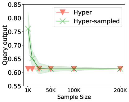
(a) Solution quality

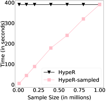
(b) Running time

Figure 6. Effect of varying sample size on HypeR-sampled output and running time for German-Syn (1M) dataset

5.3. What-If Real World Use Cases

$${{\textsc{Use}}}\ D~{}~{}{\textsc{Update}}(B)=b~{}~{}{\textsc{Output}}\ {\tt\textsc{Count}}(Credit=Good)~{}~{}{\textsc{ For}}\ {\tt{\textsc{Pre}}}(A)=a$$

(a) What-if query (German dataset): What fraction of individuals will have good credit if $B$ is updated to $b$?

$${{\textsc{Use}}}\ D\quad\quad{\textsc{Update}}(B)=b\quad\quad{\textsc{Output}}\ {\tt\textsc{Count}}(*)$$

$${\textsc{ For}}\ {\textsc{Post}}(Income)>50k~{}{\tt\textsc{And}}\ {\tt{\textsc{Pre}}}(A)=a$$

(b) What-if query (Adult dataset): How many individuals with attribute $A=a$ will have income $\geq 50K$ if $B$ is updated to $b$?

Figure 7. What-if queries for real world use cases

Table 1. Average Runtime in seconds for Count query to evaluate the effect of a hypothetical update on target for what-if queries. The time in (..) in the last row is by HypeR(-NB)-sampled, which takes the same time as HypeR(-NB) on all other datasets with $<100k$ tuples.

Dataset	Att. [$\#$]	Rows[$\#$]	HypeR	HypeR-NB	Indep
Adult (Adult, )	15	32k	45s	105s	3s
German (Dua2019, )	21	1k	1.2s	12.5s	0.4s
Amazon (HeM16, )	5,3	3k, 55k	1.7s	10.5s	0.8s
Student-syn	3,6	10k,50k	4.5s	12.3s	1.2s
German-Syn (20k)	6	20k	7.2s	22.45s	1.4s
German-Syn (1M)	6	1M	390s (44.5s)	1173s (132s)	73s

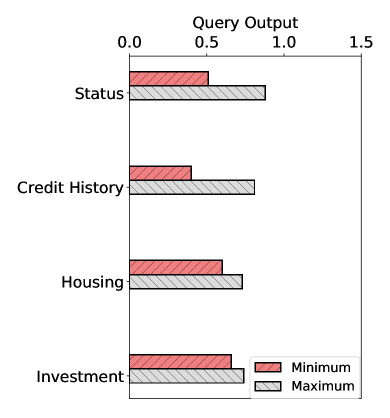
(a) German

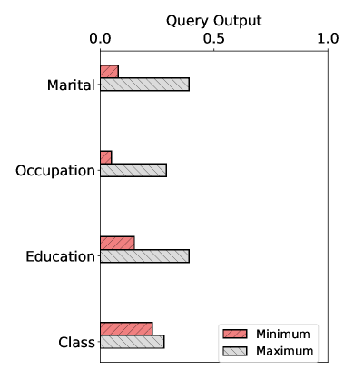
(b) Adult

Figure 8. What-if query output for German and Adult datasets on updating each attribute to their min and max values; a larger gap denotes higher attribute importance.

In this experiment, we evaluate the output of HypeR  on a diverse of hypothetical queries on various real-world datasets. Due to the absence of ground-truth, we discuss the coherence of our observations with intuitions from existing literature.

German. We considered a hypothetical update of fixing attributes ‘Status’, ‘Credit history’, and ‘housing’ to their respective minimum and maximum values to evaluate the effect of these attributes on individual credit. Figure 7(a) demonstrates the query template where $X,x,X_{2},x_{2}$ are varied to evaluate the effect of different updates. Whenever status or credit history are updated to the maximum value, more than $81\%$ of the individuals have good credit. Similarly, updating these attributes to the minimum value reduces the credit rating of more than $30\%$ individuals. On the other hand, updating other attributes like ‘housing’ and ‘investment’ affects the credit score of less than $20\%$ individuals. Figure 8(a) presents the effect of updating these attributes to their minimum and maximum value. Larger gap in the query output for Status and credit history shows that these attributes have a higher impact on credit score. We also tested the effect of updating pairs of attributes and observed that updating ‘credit history’ and ‘status’ at the same time can affect the credit score of more than $70\%$ individuals. These observations are consistent with our intuitions that credit history and account status have the maximum impact of individual credit.

Adult. This dataset has been widely studied in the fairness literature to understand the impact of individual’s gender on their income. It has a peculiar inconsistency where married individuals report total household income demonstrating a strong causal impact of marital status on their income (DBLP:conf/sigmod/SalimiGS18, ; TAGH+17, ; 10.1109/ICDM.2011.72, ). We ran a hypothetical what-if query to analyze the fraction of high-income individuals when everyone is married (Figure 7(b)). We observed that $38\%$ of the individuals have more than $50$K salary. Similarly, if all individuals were unmarried or divorced, less than $9\%$ individuals have salary more than $50$K. This wide gap in the fraction of high-income individuals for two different updates of marital status demonstrate its importance to predict household income. Figure 8(b) shows the effect of updating the attributes with the minimum or the maximum value in their domain. Additionally, updating class of all individuals has a smaller impact on the fraction with higher income. These observations match the observations of existing literature (GalhotraPS21, ), where marital status, occupation and education have the highest influence on income.

Amazon. We evaluated the effect of changing price of products of different brands on their rating. When all products have price more than the $80^{th}$ percentile, around $32\%$ of the products have average rating of more than $4$. On further reducing the laptop prices to $60^{th}$ and $40^{th}$ percentiles, more than $60\%$ of the products get an average rating of more than $4$. This shows that reducing laptop price increases average product ratings. Among different brands, we observed that Apple laptops have the maximum increase in rating on reducing laptop prices, followed by Dell, Toshiba, Acer and Asus. These observations are consistent with previous studies on laptop brands (amazonstudy, ), which mention Apple as the top-quality brand in terms of quality, customer support, design, and innovation.

5.4. Solution Quality Comparison

In this experiment, we analyzed the quality of the solution generated by HypeR with respect to the ground truth and baselines over synthetic datasets. The ground truth values are calculated using the structural equations of the causal DAG for the synthetic data.

What-if. For the German-Syn (1M) dataset, Figure 10(a) presents the output of a query that updates different attributes related to individual income and evaluates the probability of achieving good credit. For all attributes, HypeR, HypeR-sampled, and HypeR-NB estimate the query output accurately with an error margin of less than $5\%$. In contrast, Indep baseline ignores the causal structure and relies on correlation between attributes to evaluate the output. Since, the individuals with high status are highly correlated with good credit, Indep incorrectly outputs that updating Status would automatically improve credit for most of the individuals.

For the Student-Syn dataset, Figure 10(b) presents the average grade of individuals on updating different attributes that are an indicator of their academic performance. In all cases, HypeR and HypeR-NB output is accurate while Indep is confused by correlation between attributes and outputs noisy results. In addition to these hypothetical updates, we considered complex what-if queries that analyzed the effect of assignment and discussion attributes on individuals that read announcements and have high attendance. In these individuals, we observed that improving assignment score has the maximum effect on overall grade of individuals.

How-to. For the German-Syn (20k) dataset, we considered a how-to query that aims to maximize the fraction of individuals receiving good credit. We provided Status, Savings, Housing and Credit amount as the set of attributes in the HowToUpdate operator. HypeR returned that updating two attributes i) account status, and ii) housing attributes is sufficient to achieve good credit. This showed that updating a single attribute would not maximize the fraction of individuals with good credit. We evaluated the ground truth (Opt-HowTo) by enumerating all possible update queries and used the structural equations of the causal graph to evaluate the post-update value of the objective function for each update. We identified that HypeR’s output matches the ground truth update.

For the Student-Syn dataset, we evaluated a how-to query to maximize average grades of individuals with a budget of updating atmost one attribute. HypeR returned that improving individual attendance provide the maximum benefit in average grades. This output is consistent with ground truth calculated by evaluating the effect of all possible updates (Opt-HowTo).

Effect of discretization. HypeR bucketizes all continuous attributes before solving the integer program. In this experiment, we evaluate the effect of number of buckets on the solution quality and running time on a modified version of German-Syn (20k) dataset that contains continuous attributes. We partitioned the dataset into equi-width buckets and compared the solution returned by HypeR and the optimal solution calculated after discretization (Opt-discrete) with the ground truth solution (OptHowTo). Figure 9(a) compares the quality of HypeR and Opt-discrete as a ratio of the optimal value. We observe that the solution quality improves with the increase in the number of buckets and the returned solution is within $10\%$ of the optimal value whenever we consider more than $4$ buckets. The solution returned by Opt-discrete is similar to that of HypeR. The time taken by Opt-discrete increases exponentially with the number of buckets. In contrast, time taken by HypeR does not increase considerably as the number of variables in the integer program depends linearly on the number of buckets. This shows that running HypeR over a bucketized version of the dataset leads to competitive quality in reasonable amount of time.

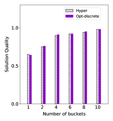
(a) Solution quality

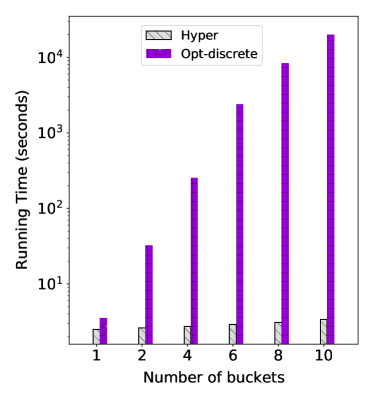
(b) Running time

Figure 9. How-to Query output for German-Syn (20k) with varying number of buckets.

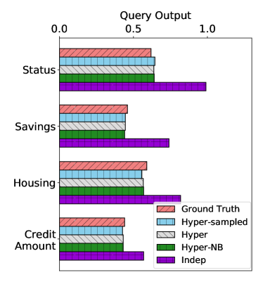
(a) German-Syn (1M)

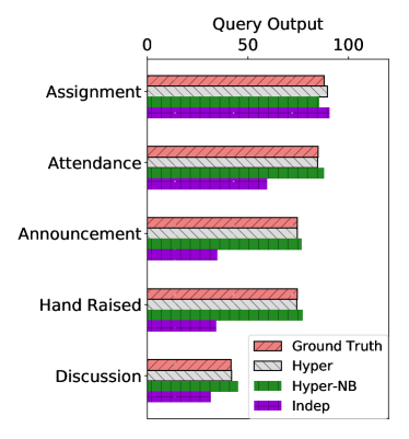
(b) Students-Syn

Figure 10. What-If Query output.

5.5. Runtime Analysis and Comparison

In this section, we evaluate the effect of different facets of the input on the runtime of HypeR. Note that our approach comprises two steps: (a) creating the aggregate view on which the query should be computed (done using a join-aggregate query), and (b) training regression functions to calculate conditional probability in the calculation of query output (the mathematical expression is in Proposition 8). This training is performed over a subset of the attributes of the view computed in the previous step. Training a regression function is more time-consuming than computing the aggregate view in step (1). Therefore, HypeR is as scalable as prior techniques for regression (we use a random forest regressor from the sklearn package). Hence the parameters we consider include (1) database size, (2) backdoor set size (see Section 3.3), and (3) query complexity. Since the effect of (1), (2) on the runtime of what-if query evaluation is directly translated to an effect on the runtime of how-to query evaluation, for how-to queries, we focus on the effect of the number of attributes in the HowToUpdate operator which will change the optimization function $\phi$ (see Section 4.3). We use the synthetic datasets German-Syn and Student-Syn.

What-if: database size. Table 1 presents the average running time to evaluate the response to a what-if query in seconds. To further evaluate the effect of database size on running time, we considered German-Syn dataset and varied the number of tuples from $10K$ to $1M$. In this experiment we consider a new variation of HypeR, denoted by HypeR-sampled, which considers a randomly chosen subset of $100K$ records for the calculation of conditional probabilities of Proposition 8. Figure 12 compares the average time taken by HypeR, HypeR-sampled with Indep for five different What-If queries and Opt-HowTo for How-to queries. We observed a linear increase in running time with respect to the dataset size for all techniques except HypeR-sampled. The increase in running time is due to the time taken to train a regressor which is used to estimate conditional probabilities for query output calculation To answer a what-if (or how-to) queries, aggregate view calculation requires less than $1\%$ of the total time. The majority of the time is spent on calculating the query output using the result in Proposition 8. Therefore, the time taken by HypeR-sampled does not increase considerably when the dataset size is increased beyond 100K.

What-if: backdoor set size. This experiment changed the background knowledge to increase the backdoor set from $2$ attributes to $6$ attributes. The running time to calculate expected fraction of high credit individuals on updating account status increased from $7.2$ seconds when backdoor set contains age and sex to $22.45$ seconds when the backdoor set contains all attributes.

What-if: query complexity. In this experiment, we synthetically add multiple attributes in the Student-syn dataset and the different operators of the query to estimate their on running time.

On adding multiple attributes in the Use operator, the time taken to compute the relevant view increases minutely. For Student-Syn, Use operator was evaluated in less than $0.5$ seconds when $5$ different attributes are added from other datasets. The increase in these attributes do not affect the running time of subsequent steps unless the attributes in For operator increase.

We now compare the effect of adding multiple attributes in the For  operator of a Count query. Adding conditions involving Pre value of randomly chosen attributes increases the number of attributes used to train the regressor, which increases the running time (Figure 11(a)). Running time increased from $4.2$ seconds when For  operator is empty to $12.1$ seconds and $17.7$ seconds when it contains $5$ and $10$ attributes, respectively. In contrast, Indep is more efficient as it does not use additional attributes to compute query output. However, if the added attribute is in the backdoor set, then the output is evaluated faster. To understand the effect of adding such attributes, we considered a query where the backdoor set contained $10$ binary attributes. To evaluate the output, probability calculation iterated over the domain of backdoor attributes and required $49.7$ seconds. The running time reduced to $7.4$ seconds when $5$ conditions on these attributes are added to the For operator.

How-to: query complexity. Figure 11(b) presents the effect of the number of attributes in HowToUpdate operator on the time taken to process the query. Increasing attributes leads to a linear increase in the number of variables in the integer program. Therefore, the time taken by HypeR increases from $7$ seconds for $5$ attributes in HowToUpdate operator to $20$ seconds for $10$ attributes. In contrast, Opt-HowTo considers all possible combinations of attribute values in the domain of attributes in the HowToUpdateoperator. It takes around $4$minutes for $5$ attributes and more than $90$ minutes for $10$ attributes. This shows that the Integer Program based optimization provides orders of magnitude improvement in running time.

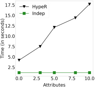
(a) What-if ( For operator)

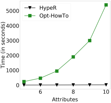
(b) How-to (HowToUpdate)

Figure 11. Running Time comparison on varying number of attributes in different operators for Student-Syn dataset.

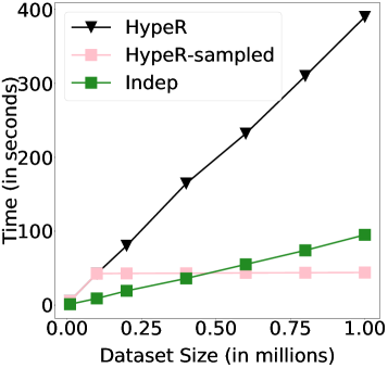
(a) What-if query

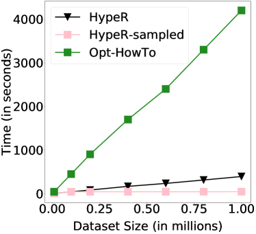
(b) How-to query

Figure 12. Running Time comparison on varying dataset size for German-Syn dataset averaged over five different queries.

6. related work

Here we review relevant literature in hypothetical reasoning in databases, probabilistic databases, and causality. The main distinction of this paper from previous work is a framework that allows for hypothetical reasoning over relational databases using a post-update distribution over possible worlds that is able to capture both direct and indirect probabilistic dependencies between attributes and tuples using a probabilistic relational causal model.

Previous work has focused on What-if and How-to analysis mainly in terms of provenance and view updates. Due to its practicality, and real applications like evaluating business strategies, there have been several works that developed support for hypothetical what-if reasoning in SQL, OLAP, and map-reduce environments (BalminPP00, ; LakshmananRS08, ; ZhouC09, ; HerodotouB11, ; NievaSS20, ). What-if reasoning through provenance updates have been studied in (DeutchIMT13, ; DeutchMT15, ; ArabG17, ; DeutchMR19, ) to efficiently measure the direct effect of updating values in the database on a view created by the query. Nguyen et. al. (Nguyen0WZYTS18, ) study the problem of efficiently performing what-if analysis with conflicting goals using data grids. Other works have considered models for hypothetical reasoning in temporal databases (ArenasB02, ; HartmannFMRT19, ), where Arenas et. al. (ArenasB02, ) focused on a logical model in which each transaction updates the database and the goal is to answer a query about the generated sequence of states, without performing the update on the whole database, and GreyCat (HartmannFMRT19, ) focused on time-evolving graphs. Christiansen et. al. (ChristiansenA98, ) propose an approach that considers a single possible world and then modifies the query evaluation procedure within a logic-based framework. Another part of hypothetical reasoning is how-to queries which have been explored mostly in terms of provenance updates (MeliouGS11Reverse, ; MeliouGS11, ; MeliouS12, ) that compute their results with hypothetical updates modeled as a Mixed Integer Program. MCDB (JampaniXWPJH08, ) allows users to create an uncertain database that has randomly generated values in the attributes or tuples (that may be correlated with other attributes or tuples). These are generated using variable generation functions that can be arbitrarily complex. It then evaluates queries over this database using Monte Carlo simulations. Eisenreich et. al. (EisenreichR10, ) propose a data analysis system allowing users to input attribute-level uncertainty and correlations using histograms and then perform operations on the data such as aggregating or filtering uncertain values. We note that uncertainty in databases has been studied in previous work on probabilistic databases (AgrawalBSHNSW06, ; DalviS07, ; AntovaKO07a, ; DalviRS09, ; Suciu20, ) where each tuple or value has a probability or confidence level attached to it, and in stochastic package queries (BrucatoYAHM20, ) that allow for optimization queries on stochastic attributes. We adapt and use the concept of block-independent database model from probabilistic databases (ReS07, ; DalviRS09, ) in this paper. The framework suggested in this paper uses a probabilistic relational causal model (SalimiPKGRS20, ) to model updates as interventions and generate the post-update distribution that describes the dependencies between the attributes and tuples. There is a vast literature on observational causal inference on stored data in AI and Statistics (e.g., (greenland1999relation, ; robins1989probability, ; greenland1999epidemiology, ; tian2000probabilities, ; robertson1996common, ; cox1984probability, ; pearl2009causality, ; angrist1996identification, ; rubin2005causal, )), and we use standard techniques from this literature to compute query output.

7. conclusions

We have defined a probabilistic model for hypothetical reasoning in relational databases. While the post-update distribution can stem from any probabilistic model, we focus here on causal models. We develop HypeR: a novel framework that supports what-if and how-to queries and performs hypothetical updates on the database, measures their effect, and computes the query results. Our framework includes new SQL-like operators to support these queries for testing a wide variety of hypothetical scenarios. We prove that the results of our queries can be computed using causal inference and we further devise an optimizations by block-independent decompositions. We show that our approach provides query results that are rational and account for implicit dependencies in the database. In future work, we plan to add support for multi-attribute updates consisting of dependent attributes and also account for database constraints and other semantic constraints. Extensions to cyclic dependencies of attributes in causal graphs is an intriguing future work. One idea that can be explored is ‘unfolding’ cyclic dependencies between attributes A and B by using a time component on attributes, and adding edges from $A[t]$ to $B[t^{\prime}]$ and $B[t]$ to $A[t^{\prime}]$ where time $t^{\prime}>t$ (called ‘chain graphs’, e.g., (DBLP:conf/uai/ShermanS19, ; ogburn2020causal, )). We also plan to develop an interactive UI where users can pose and explore hypothetical queries.

Appendix A Appendix: Computation of What-if queries and Proofs

The computation of what-if queries in the most general form uses a number of techniques including decomposable aggregates, block-independent decompositions (when available), and causal graphs (when available) and backdoor condition from the causal inference literature. For readability, we decompose the computations and their correctness proofs in the following steps:

1. (Section A.1) Computation of what-if queries for a single-relation database with a block-independent decomposition can be reduced to computation of (modified) what-if queries on individual blocks using properties of decomposble aggregate functions (see Proposition 1). This step is omitted if there are no block-independent decomposition, i.e., if the entire database forms a single block.

2. (Section A.2) Computation of what-if queries for a single block within a single-relation database. This calculation leverages the causal graph $G$ and the set of attributes that satisfy the backdoor criterion to estimate the query output for a block.

3. (Section A.3) Extends the analysis of single-relation database to multi-relation database.

4. (Section A.4) Presents the key ideas used to estimate the conditional probability distribution from the original database $D$ in our algorithms.

A.1. Reduction from Block-Independent Decomposition to Individual Blocks

First we give a proof that the computation of a what-if query can be computed as the aggregate of the results of what-if queries over each block where the database $D$ has a single relation $R$, such that both the update attribute $B$ and the outcome attribute $Y$ belong to $\texttt{Attr}(R)$ for any given what-if query $Q$. In particular, on such a database, we can assume without loss of generality that the relevant view ${{\mathcal{V}}^{rel}}=R=D$, although some of the attributes of $R$ may not be used in the second part of query $Q$. Further, both the update attribute $B$ and the outcome attribute $Y$ belong to $\texttt{Attr}(R)$. In Section A.2 we show how what-if queries are answered on each block that cannot be decomposed further.

Proposition 0.

Given a single-relation database $D=R={{\mathcal{V}}^{rel}}$ containing both the update attribute $B$ and outcome attribute $Y$, its block-independent decomposition $\mathcal{B}=\{D_{1},\ldots,D_{\ell}\}$, and a what-if query $Q$ whose result on a possible world $I\in PWD(D)$ is ${{{\tt val}}_{\tt whatif}}(Q,D,I)=aggr(\{Y_{I}[t]~{}\mathrel{\mathop{\mathchar 58\relax}}~{}{\mu}_{{\textsc{ For}}}(t)=true,t\in{{\mathcal{V}}^{rel}}\})$ (Definition 2), if $aggr$ is a decomposable function, i.e., if there exist functions $g$ and $f^{\prime}_{Q,D}$ according to Definition 5, then

(10) $${{{\tt val}}_{\tt whatif}}(Q,D)=g(\{{{{\tt val}}_{\tt whatif}}(Q^{\prime},D_{i})~{}\mathrel{\mathop{\mathchar 58\relax}}~{}\forall D_{i}\in\mathcal{B}\})$$

where $Q^{\prime}$ is the same query as $Q$ with $f^{\prime}_{Q,D}$ replacing $aggr$, $\overline{PWD}(D_{i})$ denotes the possible worlds for tuples in $D_{i}$, and

(11) $${{{\tt val}}_{\tt whatif}}(Q^{\prime},D_{i})=\mathbb{E}_{I_{i}\in\overline{PWD}(D_{i})}[{{{\tt val}}_{\tt whatif}}(Q^{\prime},D_{i},I_{i})]$$

Proof.

Recall the query result in Definition 3:

$${{{\tt val}}_{\tt whatif}}(Q,D)=\mathbb{E}_{I\in PWD(D)}[{{{\tt val}}_{\tt whatif}}(Q,D,I)]$$

(12) $$=\sum_{I\in PWD(D)}{\tt\mathrm{Pr}}_{D,U}(I)\times{{{\tt val}}_{\tt whatif}}(Q,D,I)$$

Using the assumption that ${{{\tt val}}_{\tt whatif}}(Q,D,I)=g(\{{{{\tt val}}_{\tt whatif}}(Q^{\prime},D_{i},I_{i})~{}\mathrel{\mathop{\mathchar 58\relax}}~{}I_{i}\in\mathcal{B}_{I}\})$, we get the following.

(13) $$\scriptsize{{{\tt val}}_{\tt whatif}}(Q,D)=\sum_{I\in PWD(D)}\left({\tt\mathrm{Pr}}_{D,U}(I)\cdot g(\{{{{\tt val}}_{\tt whatif}}(Q^{\prime},D_{i},I_{i})~{}\mathrel{\mathop{\mathchar 58\relax}}~{}I_{i}\in\mathcal{B}_{I}\})\right)$$

Assuming block-level independence, we substitute ${\tt\mathrm{Pr}}_{D,U}(I)$ for $\prod_{I_{i}\in\mathcal{B}_{I}}{\tt\mathrm{Pr}}_{D_{i},U}(I_{i})$, where ${\tt\mathrm{Pr}}_{D_{i},U}$ denotes the post-update probability distribution of $D_{i}$. Therefore,

(14) $$(\ref{eq:13}) =\sum_{I\in PWD(D)}\left(\left(\prod_{I_{j}\in\mathcal{B}_{I}}{\tt\mathrm{Pr}}_{D_{j},U}(I_{j})\right)\left(g(\{{{{\tt val}}_{\tt whatif}}(Q^{\prime},D_{i},I_{i})~{}\mathrel{\mathop{\mathchar 58\relax}}~{}I_{i}\in\mathcal{B}_{I}\})\right)\right) =\sum_{I\in PWD(D)}g\left(\left\{\left(\prod_{I_{j}\in\mathcal{B}_{I}}{\tt\mathrm{Pr}}_{D_{j},U}(I_{j})\right){{{\tt val}}_{\tt whatif}}(Q^{\prime},D_{i},I_{i})~{}\mathrel{\mathop{\mathchar 58\relax}}~{}I_{i}\in\mathcal{B}_{I}\right\}\right)$$

Note that for the second transition, we used the property of function $g$ in Definition 5: $\alpha g(\{x_{1},\ldots,x_{l}\})=g(\{\alpha x_{1},\ldots,\alpha x_{l}\})$, $\forall\alpha\geq 0$.

Now, suppose that for the block $I_{i}\in\mathcal{B}_{I}$ of $I\in PWD(D)$, the corresponding block in $D$ is $D_{i}\in\mathcal{B}_{D}$, with tuples having the same key.
Separating out ${\tt\mathrm{Pr}}_{D_{i},U}(I_{i})$ from $\prod_{I_{j}\in\mathcal{B}_{I}}{\tt\mathrm{Pr}}_{D_{j},U}(I_{j})$, we get the following.

(15) $$=\sum_{I\in PWD(D)}g\left\{\left(\left(\prod_{I_{j}\in\mathcal{B}_{I}\setminus\{I_{i}\}}{\tt\mathrm{Pr}}_{D_{j},U}(I_{j})\right)\times{\tt\mathrm{Pr}}_{D_{i},U}(I_{i})\times{{{\tt val}}_{\tt whatif}}(Q^{\prime},D_{i},I_{i})\right)~{}\mathrel{\mathop{\mathchar 58\relax}}~{}~{}I_{i}\in\mathcal{B}_{I}\right\}$$

(16) $$=\sum_{I\in PWD(D)}g\left\{\left(\left(\prod_{I_{j}\in\mathcal{B}_{I}\setminus\{I_{i}\}}{\tt\mathrm{Pr}}_{D_{j},U}(I_{j})\right)\times{\tt\mathrm{Pr}}_{D_{i},U}(I_{i})\times{{{\tt val}}_{\tt whatif}}(Q^{\prime},D_{i},I_{i})\right)~{}\mathrel{\mathop{\mathchar 58\relax}}~{}\forall D_{i}\in\mathcal{B}_{D}\right\}$$

(17) $$=g\left\{\sum_{I\in PWD(D)}\left(\left(\prod_{I_{j}\in\mathcal{B}_{I}\setminus\{I_{i}\}}{\tt\mathrm{Pr}}_{D_{j},U}(I_{j})\right)\times{\tt\mathrm{Pr}}_{D_{i},U}(I_{i})\times{{{\tt val}}_{\tt whatif}}(Q^{\prime},D_{i},I_{i})\right)~{}\mathrel{\mathop{\mathchar 58\relax}}~{}\forall D_{i}\in\mathcal{B}_{D}\right\}$$

In the last step, we used the property of function $g$ from Definition 5: $g(\{x_{1},\ldots,x_{l}\})+g(\{y_{1},\ldots,y_{l}\})=g(\{x_{1}+y_{1},\ldots,x_{l}+y_{l}\})$.
Substituting $PWD(D)$ as the Cartesian product of $\overline{PWD}(D_{k})$ over blocks, $PWD(D)=\bigtimes_{D_{k}\in\mathcal{B}_{D}}\overline{PWD}(D_{k})$, hence,

(18) $$(\ref{eq:19}) =g\left\{\sum_{\begin{subarray}{c}I\in\bigtimes_{D_{k}\in\mathcal{B}_{D}}\overline{PWD}(D_{k})\end{subarray}}\left(\left(\prod_{I_{j}\in\mathcal{B}_{I}\setminus\{I_{i}\}}{\tt\mathrm{Pr}}_{D_{j},U}(I_{j})\right)\times{\tt\mathrm{Pr}}_{D_{i},U}(I_{i})\times{{{\tt val}}_{\tt whatif}}(Q^{\prime},D_{i},I_{i})\right)~{}\mathrel{\mathop{\mathchar 58\relax}}~{}\forall D_{i}\in\mathcal{B}_{D}\right\}$$

Substituting ${\bigtimes_{D_{k}\in\mathcal{B}_{D}}\overline{PWD}(D_{k})}=\overline{PWD}(D_{i})\times\left(\bigtimes_{D_{k}\in\mathcal{B}_{D}\setminus\{D_{i}\}}\overline{PWD}(D_{k})\right)$

(19) $$=g\left\{\sum_{\begin{subarray}{c}I\in\overline{PWD}(D_{i})\times\\ \left(\bigtimes_{D_{k}\in\mathcal{B}_{D}\setminus\{D_{i}\}}\overline{PWD}(D_{k})\right)\end{subarray}}\left(\left(\prod_{I_{j}\in\mathcal{B}_{I}\setminus\{I_{i}\}}{\tt\mathrm{Pr}}_{D_{j},U}(I_{j})\right)\times{\tt\mathrm{Pr}}_{D_{i},U}(I_{i})\times{{{\tt val}}_{\tt whatif}}(Q^{\prime},D_{i},I_{i})\right)~{}\mathrel{\mathop{\mathchar 58\relax}}~{}\forall{D_{i}\in\mathcal{B}_{D}}\right\}$$

Let $I=I_{i}\cup I_{i}^{\prime}$ where $I_{i}^{\prime}\in\left(\bigtimes_{D_{k}\in\mathcal{B}_{D}\setminus\{D_{i}\}}\overline{PWD}(D_{k})\right)$.

(20) $$=g\left\{\sum_{\begin{subarray}{c}I_{i}\in\\ \overline{PWD}(D_{i})\end{subarray}}\quad\sum_{\begin{subarray}{c}I_{i}^{\prime}\in\\ \left(\bigtimes_{D_{k}\in\mathcal{B}_{D}\setminus\{D_{i}\}}\overline{PWD}(D_{k})\right)\end{subarray}}\left(\left(\prod_{I_{j}\in\mathcal{B}_{I}\setminus\{I_{i}\}}{\tt\mathrm{Pr}}_{D_{j},U}(I_{j})\right)\times{\tt\mathrm{Pr}}_{D_{i},U}(I_{i})\times{{{\tt val}}_{\tt whatif}}(Q^{\prime},D_{i},I_{i})\right)~{}\mathrel{\mathop{\mathchar 58\relax}}~{}\forall{D_{i}\in\mathcal{B}_{D}}\right\}$$

Separating out the terms that depend on $D_{i}$ and $I_{i}$ from the rest.

(21) $$=g\left\{\sum_{\begin{subarray}{c}I_{i}\in\\ \overline{PWD}(D_{i})\end{subarray}}\left(\left({\tt\mathrm{Pr}}_{D_{i},U}(I_{i})\times{{{\tt val}}_{\tt whatif}}(Q^{\prime},D_{i},I_{i})\right)\quad\times\sum_{\begin{subarray}{c}I_{i}^{\prime}\in\\ \left(\bigtimes_{D_{k}\in\mathcal{B}_{D}\setminus\{D_{i}\}}\overline{PWD}(D_{k})\right)\end{subarray}}\left(\prod_{I_{j}\in\mathcal{B}_{I}\setminus\{I_{i}\}}{\tt\mathrm{Pr}}_{D_{j},U}(I_{j})\right)\right)~{}\mathrel{\mathop{\mathchar 58\relax}}~{}\forall{D_{i}\in\mathcal{B}_{D}}\right\}$$

Blocks $I_{j}\in\mathcal{B}_{I}\setminus\{I_{i}\}$ are independent. Therefore, $\left(\prod_{I_{j}\in\mathcal{B}_{I}\setminus\{I_{i}\}}{\tt\mathrm{Pr}}_{D_{j},U}(I_{j})\right)={\tt\mathrm{Pr}}_{D\setminus D_{i},U}(I_{i}^{\prime})$, where $I_{i}^{\prime}=\cup_{I_{j}\in\mathcal{B}_{I}\setminus\{I_{i}\}}I_{j}$, which denotes the post-update probability of all blocks except $I_{i}$. Hence,

(22) $$(\ref{eq:24}) =g\left\{\sum_{\begin{subarray}{c}I_{i}\in\\ \overline{PWD}(D_{i})\end{subarray}}\left(\left({\tt\mathrm{Pr}}_{D_{i},U}(I_{i})\times{{{\tt val}}_{\tt whatif}}(Q^{\prime},D_{i},I_{i})\right)\quad\times\sum_{\begin{subarray}{c}I_{i}^{\prime}\in\\ \left(\bigtimes_{D_{k}\in\mathcal{B}_{D}\setminus\{D_{i}\}}\overline{PWD}(D_{k})\right)\end{subarray}}\left({\tt\mathrm{Pr}}_{D\setminus D_{i},U}(I_{i}^{\prime})\right)\right)~{}\mathrel{\mathop{\mathchar 58\relax}}~{}\forall{D_{i}\in\mathcal{B}_{D}}\right\}$$

Since $\sum_{\begin{subarray}{c}I_{i}^{\prime}\in\left(\bigtimes_{D_{k}\in\mathcal{B}_{D}\setminus\{D_{i}\}}\overline{PWD}(D_{k})\right)\end{subarray}}\left({\tt\mathrm{Pr}}_{D\setminus D_{i},U}(I_{i}^{\prime})\right)$ is $1$ (the sum of probabilities of possible worlds of all blocks except $D_{i}$),

(23) $$(\ref{eq:22}) =g(\{\sum_{\begin{subarray}{c}I_{i}\in\overline{PWD}(D_{i})\end{subarray}}\left({\tt\mathrm{Pr}}_{D_{i},U}(I_{i})\times{{{\tt val}}_{\tt whatif}}(Q^{\prime},D_{i},I_{i})\right)~{}\mathrel{\mathop{\mathchar 58\relax}}~{}\forall D_{i}\in\mathcal{B}_{D}\})$$

Notice that the term $\sum_{\begin{subarray}{c}I_{i}\in\overline{PWD}(D_{i})\end{subarray}}\left({\tt\mathrm{Pr}}_{D_{i},U}(I_{i})\times{{{\tt val}}_{\tt whatif}}(Q^{\prime},D_{i},I_{i})\right)$ denotes the expected value of $f^{\prime}_{Q,D_{i}}$ over the post-update distribution, denoted by $\mathbb{E}_{I_{i}\in\overline{PWD}(D_{i})}[{{{\tt val}}_{\tt whatif}}(Q^{\prime},D_{i},I_{i})]$, and thus ${{{\tt val}}_{\tt whatif}}(Q^{\prime},D_{i})=\mathbb{E}_{I_{i}\in\overline{PWD}(D_{i})}[{{{\tt val}}_{\tt whatif}}(Q^{\prime},D_{i},I_{i})]$, and ${{{\tt val}}_{\tt whatif}}(Q,D)=g(\{{{{\tt val}}_{\tt whatif}}(Q^{\prime},D_{i})~{}\mathrel{\mathop{\mathchar 58\relax}}~{}\forall D_{i}\in\mathcal{B}\})$ as stated in the proposition. ∎

A.2. Computation for a single-block

In this section we show how to compute ${{{\tt val}}_{\tt whatif}}(Q^{\prime},D_{i})$ using the causal graph of the block $D_{i}$ given a (possibly modified) what-if query $Q^{\prime}$. First, in Section A.2.1, we consider the case where the predicate in the For operator ($\mu_{{\textsc{ For}}}$) is a disjunction of different For sub-operators explained below. We then show that a For clause that does not satisfy a disjoint property can be modified using the principle of inclusion-exclusion. Lastly, we show that any For clause can be represented as a disjunction that satisfies these properties in Section A.2.4.

A.2.1. For operator has Disjunction of Conjunctions of Pre and Post operators, and $Agg={\tt\textsc{Count}}$ in the what-if query

Here we assume that the aggregate operator $Agg={\tt\textsc{Count}}$ in the what-if query. Further, we assume that the For operator ($\mu_{{\textsc{ For}}}$) is a disjunction of different For sub-operators denoted by $\lor_{k}{\mu}_{{\textsc{ For}}}^{k}$ and these sub-operators satisfy the following conditions.

1. Each sub-operator ${\mu}_{{\textsc{ For}}}^{k}$ can be decomposed into a conjunction over two For clauses, one denoting For condition on pre-update values of the tuples, and the other referring to the post-update values of the tuples. This condition is required to separate out the conditions applied by the For operator on the original/pre-update value of a tuple $t\in D$ and its post-update values.

2. Disjointness: Each pair of tuple (t,t’), where $t\in D,t^{\prime}\in I$ for any $I\in PWD(D)$ satisfies at most one of the sub-operators ${\mu}_{{\textsc{ For}}}^{k}$.

For example, consider a For clause,

$$\left({\tt{\textsc{Pre}}}(A_{1})=1\right)\lor\left({\tt{\textsc{Pre}}}(A_{1})\in\{2,3,4\}\wedge{\textsc{Post}}(A_{2})=2\right)\lor\left({\tt{\textsc{Pre}}}(A_{1})>4\wedge{\textsc{Post}}(A_{2})=5\right).$$

It consists of three different sub-clauses separated by disjunctions: (a) ${\tt{\textsc{Pre}}}(A_{1})=1$, (b) ${\tt{\textsc{Pre}}}(A_{1})\in\{2,3,4\}\wedge{\textsc{Post}}(A_{2})=2$, and (c) ${\tt{\textsc{Pre}}}(A_{1})>4\wedge{\textsc{Post}}(A_{2})=5$. In this case a tuple $t\in D$ and its post-update tuple $t^{\prime}\in I$ can satisfy only one of the three sub-clauses.

(A) Computation of what-if query in a block in terms of the post-update probabilities of tuples.  Proposition 2 shows how the computation in each block is done by the post-update probabilities, which we further reduce to pre-update probabilities in step (B) below. To prove Proposition 2, we augment the notation presented in Definition 2 for the For operator to be more fine-grained and define ${\mu}_{{\textsc{ For}},{\tt{\textsc{Pre}}}}$ and ${\mu}_{{\textsc{ For}},{\textsc{Post}}}$ as the conditions in the For operator that are defined with the Pre and Post operators, respectively. The Boolean representation of disjoint For clauses is denoted as $\lor_{k}({\mu}_{{\textsc{ For}},{\tt{\textsc{Pre}}}}^{k}\wedge{\mu}_{{\textsc{ For}},{\textsc{Post}}}^{k})$ where any tuple $t\in D$ and the corresponding tuple $t^{\prime}$ sharing the same key (denoted by ${\mathbf{key}}[t]={\mathbf{key}}[t^{\prime}]$, where ${\mathbf{key}}$ refers to all attributes defining the primary key of the tuple) in any possible world $I\in PWD(D)$ satisfies at most one of the sub-clauses $({\mu}_{{\textsc{ For}},{\tt{\textsc{Pre}}}}^{k}\wedge{\mu}_{{\textsc{ For}},{\textsc{Post}}}^{k})$.

Proposition 0.

Given a single-relation database $D$ with its block independent decomposition $\mathcal{B}_{D}$, a block $D_{i}\in\mathcal{B}_{D}$, a ground causal graph $G$, a what-if query $Q^{\prime}$ where $Agg={\tt\textsc{Count}}$, and For operator is denoted by ${\mu}_{{\textsc{ For}}}$ where ${\mu}_{{\textsc{ For}}}$ can be represented as a disjunction of conjunction of disjoint For conditions, $\lor_{k}({\mu}_{{\textsc{ For}},{\tt{\textsc{Pre}}}}^{k}\wedge{\mu}_{{\textsc{ For}},{\textsc{Post}}}^{k})$, the following holds.

(24) $${{{\tt val}}_{\tt whatif}}(Q^{\prime},D_{i})=\sum_{t\in D_{i}}\left(\sum_{k}\left({\tt\mathrm{Pr}}_{D_{i},U}({\mu}_{{\textsc{ For}},{\textsc{Post}}}^{k}(t)={\tt true}|{\mu}_{{\textsc{ For}},{\tt{\textsc{Pre}}}}^{k}(t)={\tt true})\right)\right)$$

In this equation, ${\tt\mathrm{Pr}}_{D_{i},U}(\mu_{{\textsc{ For}},{\textsc{Post}}}^{k}(t)={\tt true}|{\mu}_{{\textsc{ For}},{\tt{\textsc{Pre}}}}^{k}(t)={\tt true})$ denotes the sum of probabilities of all possible worlds of $D_{i}$ such that the tuple $t$ that satisfied ${\mu}_{{\textsc{ For}},{\tt{\textsc{Pre}}}}^{k}(t)={\tt true}$ before the update $U$ also satisfies ${\mu}_{{\textsc{ For}},{\textsc{Post}}}^{k}(t)$ after the update.

Proof.

Using equation (5) in Proposition 7, we expand ${{{\tt val}}_{\tt whatif}}(Q^{\prime},D_{i})$ as follows. Here $\mathbbm{1}$ denotes the indicator function.

(25) $${{{\tt val}}_{\tt whatif}}(Q^{\prime},D_{i}) =\mathbb{E}_{I_{i}\in\overline{PWD}(D_{i})}[{{{\tt val}}_{\tt whatif}}(Q^{\prime},D_{i},I_{i})]$$

(26) $$=\sum_{\begin{subarray}{c}I_{j}\in\overline{PWD}(D_{i})\end{subarray}}\left({\tt\mathrm{Pr}}_{D_{i},U}(I_{j})\times{{{\tt val}}_{\tt whatif}}(Q^{\prime},D_{i},I_{j})\right)$$

(27) $$=\sum_{\begin{subarray}{c}I_{j}\in\overline{PWD}(D_{i})\end{subarray}}\left({\tt\mathrm{Pr}}_{D_{i},U}(I_{j})\times\sum_{t\in D_{i},t^{\prime}\in I_{j}~{}\mathrel{\mathop{\mathchar 58\relax}}~{}{\mathbf{key}}[t]={\mathbf{key}}[t^{\prime}]}\left(\mathbbm{1}\{\lor_{k}\left({\mu}_{{\textsc{ For}},{\tt{\textsc{Pre}}}}^{k}(t)={\tt true}\wedge{\mu}_{{\textsc{ For}},{\textsc{Post}}}^{k}(t^{\prime})={\tt true}\right)\}\right)\right)$$

Since $\lor_{k}({\mu}_{{\textsc{ For}},{\tt{\textsc{Pre}}}}^{k}\wedge{\mu}_{{\textsc{ For}},{\textsc{Post}}}^{k})$ consists of disjoint For conjunctive predicates, a pair of tuples $(t,t^{\prime})$ having the same ${\mathbf{key}}$ can satisfy atmost one of the sub-predicates. Therefore, $\left(\mathbbm{1}\{\lor_{k}\left({\mu}_{{\textsc{ For}},{\tt{\textsc{Pre}}}}^{k}(t)={\tt true}\wedge{\mu}_{{\textsc{ For}},{\textsc{Post}}}^{k}(t^{\prime})={\tt true}\right)\}\right)$ can be written as a sum of different indicator random variables.

(28) $$=\sum_{\begin{subarray}{c}I_{j}\in\overline{PWD}(D_{i})\end{subarray}}\left({\tt\mathrm{Pr}}_{D_{i},U}(I_{j})\times\sum_{t\in D_{i},t^{\prime}\in I_{j}~{}\mathrel{\mathop{\mathchar 58\relax}}~{}{\mathbf{key}}[t]={\mathbf{key}}[t^{\prime}]}\left(\sum_{k}\mathbbm{1}\left\{{\mu}_{{\textsc{ For}},{\tt{\textsc{Pre}}}}^{k}(t)={\tt true}\wedge{\mu}_{{\textsc{ For}},{\textsc{Post}}}^{k}(t^{\prime})={\tt true}\right\}\right)\right)$$

By splitting the inner indicator into a product of the indicators of the two conjunctions and extracting the sum over $k$:

(29) $$=\sum_{\begin{subarray}{c}I_{j}\in\overline{PWD}(D_{i})\end{subarray}}\sum_{k}\left({\tt\mathrm{Pr}}_{D_{i},U}(I_{j})\times\sum_{t\in D_{i}}\left(\mathbbm{1}\{{\mu}_{{\textsc{ For}},{\tt{\textsc{Pre}}}}^{k}(t)={\tt true}\}\times\mathbbm{1}\{{\mu}_{{\textsc{ For}},{\textsc{Post}}}^{k}(t^{\prime})={\tt true},\text{where }{\mathbf{key}}[t]={\mathbf{key}}[t^{\prime}],t^{\prime}\in I^{\prime}\}\right)\right)$$

(30) $$=\sum_{t\in D_{i}}\sum_{k}\left(\mathbbm{1}\{{\mu}_{{\textsc{ For}},{\tt{\textsc{Pre}}}}^{k}(t)={\tt true}\}\times\sum_{\begin{subarray}{c}I_{j}\in\overline{PWD}(D_{i})\end{subarray}}\left({\tt\mathrm{Pr}}_{D_{i},U}(I_{j})\times\sum_{t^{\prime}\in I_{j}~{}\mathrel{\mathop{\mathchar 58\relax}}~{}{\mathbf{key}}[t]={\mathbf{key}}[t^{\prime}]}\mathbbm{1}\{{\mu}_{{\textsc{ For}},{\textsc{Post}}}^{k}(t^{\prime})={\tt true}\}\right)\right)$$

(31) $$=\sum_{t\in D_{i}}\left(\sum_{k}\mathbbm{1}\{{\mu}_{{\textsc{ For}},{\tt{\textsc{Pre}}}}^{k}(t)={\tt true}\}\times\left(\sum_{\begin{subarray}{c}I_{j}\in\overline{PWD}(D_{i})\\ t^{\prime}\in I_{j},{\mathbf{key}}[t]={\mathbf{key}}[t^{\prime}]\end{subarray}}\left({\tt\mathrm{Pr}}_{D_{i},U}(I_{j})\times\mathbbm{1}\{{\mu}_{{\textsc{ For}},{\textsc{Post}}}^{k}(t^{\prime})={\tt true}\}\right)\right)\right)$$

(32) $$=\sum_{t\in D_{i}}\left(\sum_{k}\left(\sum_{\begin{subarray}{c}I_{j}\in\overline{PWD}(D_{i})\\ t^{\prime}\in I_{j},{\mathbf{key}}[t]={\mathbf{key}}[t^{\prime}]\end{subarray}}\left({\tt\mathrm{Pr}}_{D_{i},U}(I_{j})\times\mathbbm{1}\{{\mu}_{{\textsc{ For}},{\tt{\textsc{Pre}}}}^{k}(t)={\tt true}\wedge{\mu}_{{\textsc{ For}},{\textsc{Post}}}^{k}(t^{\prime})={\tt true}\}\right)\right)\right)$$

(33) $$=\sum_{t\in D_{i}}\left(\sum_{k}\left({\tt\mathrm{Pr}}_{D_{i},U}(\mu_{{\textsc{ For}},{\textsc{Post}}}^{k}(t)={\tt true}|\mu_{{\textsc{ For}},{\tt{\textsc{Pre}}}}^{k}(t)={\tt true})\right)\right)$$

Note that if a tuple $t$ is not affected by the update, ${\tt\mathrm{Pr}}_{D_{i},U}(\mu_{{\textsc{ For}},{\textsc{Post}}}^{k}(t)={\tt true}|\mu_{{\textsc{ For}},{\tt{\textsc{Pre}}}}^{k}(t)={\tt true})=\mathbbm{1}\{\mu_{{\textsc{ For}},{\tt{\textsc{Pre}}}}^{k}(t)={\tt true}\wedge\mu_{{\textsc{ For}},{\textsc{Post}}}^{k}(t)={\tt true}\}$.

∎

(B) Reduction of post-update probability in equation (24) of Proposition 2 in terms of the causal graph of given database $D$.  The expression in equation (24) in Proposition 2 relies on the post-update probability distribution of the block $D_{i}$, denoted by ${\tt\mathrm{Pr}}_{D_{i},U}$. We now use the backdoor criterion from causal inference literature [38] to simplify these expressions and estimate the probability from the input database $D$, which we review briefly. A set of attributes ${\mathbf{C}}$ satisfies the backdoor criterion w.r.t. $B$ and $Y$ if no attribute $C\in{\mathbf{C}}$ is a descendant of $Y$ or $B$ and all paths from $B$ to $Y$ which contain an incoming edge into $Y$ are blocked by ${\mathbf{C}}$. A path is considered to be blocked by ${\mathbf{C}}$ if there is a non-collider attribute on the path that is present in ${\mathbf{C}}$ or if a collider attribute is not in ${\mathbf{C}}$ then none of the descendant of the collider is in ${\mathbf{C}}$. With the help of the backdoor criterion, we leverage the following property for our simplification [38], which reduces post-update probability ${\tt\mathrm{Pr}}_{D,U}$ to the pre-update distribution ${\tt\mathrm{Pr}}_{D}$.

(34) $$\scriptsize{\tt\mathrm{Pr}}_{D,U}(Y=y\mid B=b,{\mathbf{C}}={\mathbf{c}})={\tt\mathrm{Pr}}_{D}(Y=y\mid B=f(b),{\mathbf{C}}={\mathbf{c}})$$

where $f(b)$ denotes the post-update value of $B=b$.

Computation of blocking set $C$:  Let ${\mathbf{C}}$ denote a set of attributes that satisfy the backdoor criterion with respect to the update attribute $B$ and the attributes in ${\mu}_{{\textsc{ For}},{\textsc{Post}}}^{k}$. We use the ground causal graph $G$ to identify the minimal subset of all ancestors of $B$ and attributes in ${\mu}_{{\textsc{ For}},{\textsc{Post}}}^{k}$ that block all backdoor paths [38] by a greedy procedure: we start with all non-descendants of $B,Y$ excluding $B,Y$ as ${\mathbf{C}}$, and the remove one node at a time until we reach a minimal set for blocking that cannot be reduced further. In case $G$ is not known, we consider all attributes of all tuples in the block $D_{i}$ to satisfy the backdoor criterion.

Computation of post-update probability for $Agg={\tt\textsc{Count}}$ We will use ${\mathbf{C}}_{k}$ to denote the backdoor set for sub-predicate ${\mu}^{k}$, and ${\mathbf{c}}_{k}\in\texttt{Dom}({\mathbf{C}}_{k})$ to denote a combination of values from the domain of these nodes. Then

(35) $${\tt\mathrm{Pr}}_{D_{i},U}(\mu_{{\textsc{ For}},{\textsc{Post}}}^{k}(t)={\tt true}|\mu_{{\textsc{ For}},{\tt{\textsc{Pre}}}}^{k}(t)={\tt true})$$

(36) $$=\sum_{{\mathbf{c}}_{k}\in~{}\texttt{Dom}({\mathbf{C}}_{k})}\left({\tt\mathrm{Pr}}_{D_{i},U}({\mu}_{{\textsc{ For}},{\textsc{Post}}}^{k}(t)={\tt true}~{}|~{}{\mu}_{{\textsc{ For}},{\tt{\textsc{Pre}}}}^{k}(t)={\tt true},{\mathbf{C}}_{k}[t]={\mathbf{c}}_{k})\times{\tt\mathrm{Pr}}_{D_{i},U}({\mathbf{C}}_{k}[t]={\mathbf{c}}_{k}~{}|~{}{\mu}_{{\textsc{ For}},{\tt{\textsc{Pre}}}}^{k}(t)={\tt true})\right)$$

Since the second component only involves non-descendants of the update attribute $B$ in the set ${\mathbf{C}}_{k}$, therefore for these ${\mathbf{C}}_{k}[t]$, post-update probability ${\tt\mathrm{Pr}}_{D_{i},U}$ is the same as the pre-update probability ${\tt\mathrm{Pr}}_{D_{i}}$. Hence,

(37) $$(\ref{eq:36}) =\sum_{{\mathbf{c}}_{k}\in~{}\texttt{Dom}({\mathbf{C}}_{k})}\left({\tt\mathrm{Pr}}_{D_{i},U}({\mu}_{{\textsc{ For}},{\textsc{Post}}}^{k}(t)={\tt true}~{}|~{}{\mu}_{{\textsc{ For}},{\tt{\textsc{Pre}}}}^{k}(t)={\tt true},{\mathbf{C}}_{k}[t]={\mathbf{c}}_{k})\times{\tt\mathrm{Pr}}_{D_{i}}({\mathbf{C}}_{k}[t]={\mathbf{c}}_{k}~{}|~{}{\mu}_{{\textsc{ For}},{\tt{\textsc{Pre}}}}^{k}(t)={\tt true})\right)$$

We now use the same simplification to split the first term into two terms, using conditional probabilities with respect to the value $b$ of $B$ before the update.

$$(\ref{eq:37}) =\sum_{{\mathbf{c}}_{k}\in~{}\texttt{Dom}({\mathbf{C}}_{k})}(\sum_{b\in~{}\texttt{Dom}(B)}\left({\tt\mathrm{Pr}}_{D_{i},U}({\mu}_{{\textsc{ For}},{\textsc{Post}}}^{k}(t)={\tt true}~{}|~{}{\mu}_{{\textsc{ For}},{\tt{\textsc{Pre}}}}^{k}(t)={\tt true},B[t]=b,{\mathbf{C}}_{k}[t]={\mathbf{c}}_{k})\times{\tt\mathrm{Pr}}_{D_{i},U}(B[t]=b~{}|~{}{\mu}_{{\textsc{ For}},{\tt{\textsc{Pre}}}}^{k}(t)={\tt true},{\mathbf{C}}_{k}={\mathbf{c}}_{k})\right)$$

(38) $$\quad\quad\quad\quad\quad\quad\times{\tt\mathrm{Pr}}_{D_{i}}\left({\mathbf{C}}_{k}[t]={\mathbf{c}}_{k}~{}|~{}{\mu}_{{\textsc{ For}},{\tt{\textsc{Pre}}}}^{k}(t)={\tt true}\right))$$

Since $B[t]=b$ refers to the pre-update value of attribute $B$, the second term ${\tt\mathrm{Pr}}_{D_{i},U}(B[t]=b~{}|~{}{\mu}_{{\textsc{ For}},{\tt{\textsc{Pre}}}}^{k}(t)={\tt true},{\mathbf{C}}_{k}={\mathbf{c}}_{k})$ is the same as ${\tt\mathrm{Pr}}_{D_{i}}(B[t]=b~{}|~{}{\mu}_{{\textsc{ For}},{\tt{\textsc{Pre}}}}^{k}(t)={\tt true},{\mathbf{C}}_{k}={\mathbf{c}}_{k})$. Hence,

$$(\ref{eq:38}) =\sum_{{\mathbf{c}}_{k}\in~{}\texttt{Dom}({\mathbf{C}}_{k})}(\sum_{b\in~{}\texttt{Dom}(B)}\left({\tt\mathrm{Pr}}_{D_{i},U}({\mu}_{{\textsc{ For}},{\textsc{Post}}}^{k}(t)={\tt true}~{}|~{}{\mu}_{{\textsc{ For}},{\tt{\textsc{Pre}}}}^{k}(t)={\tt true},B[t]=b,{\mathbf{C}}_{k}[t]={\mathbf{c}}_{k})\times{\tt\mathrm{Pr}}_{D_{i}}(B[t]=b~{}|~{}{\mu}_{{\textsc{ For}},{\tt{\textsc{Pre}}}}^{k}(t)={\tt true},{\mathbf{C}}_{k}={\mathbf{c}}_{k})\right)$$

(39) $$\quad\quad\quad\quad\quad\quad\times{\tt\mathrm{Pr}}_{D_{i}}\left({\mathbf{C}}_{k}[t]={\mathbf{c}}_{k}|{\mu}_{{\textsc{ For}},{\tt{\textsc{Pre}}}}^{k}(t)={\tt true}\right))$$

Using, equation (34), we replace the post-update probability ${\tt\mathrm{Pr}}_{D_{i},U}$ in the first term with ${\tt\mathrm{Pr}}_{D_{i}}$ and $B[t]=b$ with $B[t]=f(b)$ as specified in the update $U$:

$$(\ref{eq:eq39}) =\sum_{{\mathbf{c}}_{k}\in~{}\texttt{Dom}({\mathbf{C}}_{k})}(\sum_{b\in~{}\texttt{Dom}(B)}\left({\tt\mathrm{Pr}}_{D_{i}}({\mu}_{{\textsc{ For}},{\textsc{Post}}}^{k}(t)={\tt true}~{}|~{}{\mu}_{{\textsc{ For}},{\tt{\textsc{Pre}}}}^{k}(t)={\tt true},B[t]=f(b),{\mathbf{C}}_{k}[t]={\mathbf{c}}_{k})\times{\tt\mathrm{Pr}}_{D_{i}}(B[t]=b~{}|~{}{\mu}_{{\textsc{ For}},{\tt{\textsc{Pre}}}}^{k}(t)={\tt true},{\mathbf{C}}_{k}={\mathbf{c}}_{k})\right)$$

(40) $$\quad\quad\quad\quad\quad\quad\times{\tt\mathrm{Pr}}_{D_{i}}\left({\mathbf{C}}_{k}[t]={\mathbf{c}}_{k}|{\mu}_{{\textsc{ For}},{\tt{\textsc{Pre}}}}^{k}(t)={\tt true}\right))$$

Replacing (40) in equation (33) and summing over all tuples $t$ in $D_{i}$ and all disjoint sub-predicates ${\mu}_{{\textsc{ For}},{\tt{\textsc{Pre}}}}^{k}\wedge{\mu}_{{\textsc{ For}},{\textsc{Post}}}^{k}$, we get the final expression for computing the post-update probability for $Agg={\tt\textsc{Count}}$.

Complexity The computation of (40) iterates over all values in the domain of attributes ${{\mathbf{C}}_{k}}\cup\{B\}$ and computes three different probability values for each value of these attributes. Each probability calculation expression is estimated from the input database $D$ using regression analysis and runs in time linear in the number of records under the homogeneity assumption (please see Section A.4 for more details). Additionally, ${\tt\mathrm{Pr}}_{D_{i}}\left(B[t]=b|{\mathbf{C}}_{k}[t]=c_{k},{\mu}_{{\textsc{ For}},{\tt{\textsc{Pre}}}}^{k}(t)={\tt true}\right)$ is $0$ if the original database contains no tuple with the value $c_{k}$ for ${{\mathbf{C}}_{k}}$ and $b$ for $B[t]$. Therefore, the expression contains non-zero terms only when the support of attribute values $c_{k}\in\texttt{Dom}({\mathbf{C}}_{k})$ and $b$ is non-zero. Using this property, our implementation first identifies all values in ${{\mathbf{C}}_{k}}\cup\{B\}$ that have non-zero support and ignores the rest. Therefore, the overall complexity is $O(n\times\gamma(B\cup{\mathbf{C}}_{k}))$ where the $\gamma$ function identifies values with non-zero support. This shows that $\gamma(B\cup{\mathbf{C}}_{k})<n$ (because each value has non-zero support) and $\gamma(B\cup{\mathbf{C}}_{k})<|\texttt{Dom}(B)|\times_{A\in{\mathbf{C}}_{k}}|\texttt{Dom}(A)|$ (because $\gamma$ denotes a subset of all possible values in the domain of the attributes), simplifying the overall complexity to $O(n\times\min\{n,|\texttt{Dom}(B)|\times_{A\in{\mathbf{C}}_{k}}|\texttt{Dom}(A)|\})$. Hence, the computation can be done in time polynomial in data complexity [55] (when the size of the schema and the query is fixed), but can be exponential in query complexity depending on the size of the backdoor set ${\mathbf{C}}_{k}$.

Probability distribution ${\tt\mathrm{Pr}}_{D_{i}}$ denotes the probability distribution of constructing $D_{i}$ which is dependent on the causal graph $G$. Even though the initial database $D$ is fixed, we assume that all tuples are generated homogeneously according to the causal graph.

A.2.2. Computation for $Agg=SUM$ and $AVG$

Proposition 2 showed that a disjunction of disjoint For sub-predicates translates to a summation of probability values when $Agg={\tt\textsc{Count}}$. The condition for $Agg=SUM$ and its proof are similar. We now simplify ${{{\tt val}}_{\tt whatif}}$ when $Agg=SUM$ for a single sub-predicate which consists of a conjunction of Pre and Post predicates $({\mu}_{{\textsc{ For}},{\tt{\textsc{Pre}}}}\wedge{\mu}_{{\textsc{ For}},{\textsc{Post}}})$. In general, the final value is obtained by summing over all sub-predicates $({\mu}^{k}_{{\textsc{ For}},{\tt{\textsc{Pre}}}}\wedge{\mu}^{k}_{{\textsc{ For}},{\textsc{Post}}})$ similar to (33).

Proposition 0.

Given a single-relation database $D$ and a block $D_{i}\in\mathcal{B}_{D}$ and a what-if query $Q^{\prime}$ with aggregate $Agg={\tt\textsc{Sum}}$, where the predicate in the For operator is ${\mu}_{{\textsc{ For}}}=({\mu}_{{\textsc{ For}},{\tt{\textsc{Pre}}}}\wedge{\mu}_{{\textsc{ For}},{\textsc{Post}}})$, the following holds.

(41) $${{{\tt val}}_{\tt whatif}}(Q^{\prime},D_{i})=\sum_{t\in D_{i}}\left(\sum_{y\in\texttt{Dom}(Y)}\left(y\times{\tt\mathrm{Pr}}_{D_{i},U}(Y[t]=y,\mu_{{\textsc{ For}},{\textsc{Post}}}(t)={\tt true}~{}|~{}\mu_{{\textsc{ For}},{\tt{\textsc{Pre}}}}(t)={\tt true})\right)\right)$$

Proof.

Similar to (25)-(26),

(42) $${{{\tt val}}_{\tt whatif}}(Q^{\prime},D_{i}) =\sum_{\begin{subarray}{c}I_{j}\in\overline{PWD}(D_{i})\end{subarray}}\left({\tt\mathrm{Pr}}_{D_{i},U}(I_{j})\times{{{\tt val}}_{\tt whatif}}(Q^{\prime},D_{i})\right)$$

(43) $$=\sum_{\begin{subarray}{c}I_{j}\in\overline{PWD}(D_{i})\end{subarray}}\left({\tt\mathrm{Pr}}_{D_{i},U}(I_{j})\times\sum_{t\in D_{i},t^{\prime}\in I_{j}~{}\mathrel{\mathop{\mathchar 58\relax}}~{}{\mathbf{key}}{}[t]={\mathbf{key}}{}[t^{\prime}]}\left(Y[t^{\prime}]\times\mathbbm{1}\{{\mu}_{{\textsc{ For}},{\tt{\textsc{Pre}}}}(t)={\tt true}\wedge{\mu}_{{\textsc{ For}},{\textsc{Post}}}(t^{\prime})={\tt true}\}\right)\right)$$

(44) $$=\sum_{\begin{subarray}{c}I_{j}\in\overline{PWD}(D_{i})\end{subarray}}\left({\tt\mathrm{Pr}}_{D_{i},U}(I_{j})\times\sum_{t\in D_{i}}\left(Y[t^{\prime}]\times\mathbbm{1}\{{\mu}_{{\textsc{ For}},{\tt{\textsc{Pre}}}}(t)={\tt true}\}\times\mathbbm{1}\{{\mu}_{{\textsc{ For}},{\textsc{Post}}}(t^{\prime})={\tt true},\text{where }{\mathbf{key}}{}[t]={\mathbf{key}}{}[t^{\prime}],t^{\prime}\in I^{\prime}\}\right)\right)$$

(45) $$=\sum_{t\in D_{i}}\left(\mathbbm{1}\{{\mu}_{{\textsc{ For}},{\tt{\textsc{Pre}}}}(t)={\tt true}\}\times\sum_{\begin{subarray}{c}I_{j}\in\overline{PWD}(D_{i})\end{subarray}}\left({\tt\mathrm{Pr}}_{D_{i},U}(I_{j})\times\sum_{t^{\prime}\in I_{j}~{}\mathrel{\mathop{\mathchar 58\relax}}~{}{\mathbf{key}}{}[t]={\mathbf{key}}{}[t^{\prime}]}Y[t^{\prime}]\times\mathbbm{1}\{{\mu}_{{\textsc{ For}},{\textsc{Post}}}(t^{\prime})={\tt true}\}\right)\right)$$

(46) $$=\sum_{t\in D_{i}}\left(\mathbbm{1}\{{\mu}_{{\textsc{ For}},{\tt{\textsc{Pre}}}}(t)={\tt true}\}\times\sum_{\begin{subarray}{c}I^{\prime}\in\overline{PWD}_{D_{i}}\\ t^{\prime}\in I^{\prime},{\mathbf{key}}{}[t]={\mathbf{key}}{}[t^{\prime}]\end{subarray}}Y[t^{\prime}]\times\left({\tt\mathrm{Pr}}_{D_{i},U}(I^{\prime})\times\mathbbm{1}\{{\mu}_{{\textsc{ For}},{\textsc{Post}}}(t^{\prime})={\tt true}\}\right)\right)$$

(47) $$=\sum_{t\in D_{i}}\left(\sum_{y\in\texttt{Dom}(Y)}\left(y\times{\tt\mathrm{Pr}}_{D_{i},U}(Y[[t]=y,\mu_{{\textsc{ For}},{\textsc{Post}}}(t)={\tt true}~{}|~{}\mu_{{\textsc{ For}},{\tt{\textsc{Pre}}}}(t)={\tt true})\right)\right)$$

∎

The post-update probability distribution ${\tt\mathrm{Pr}}_{D_{i},U}$ can be estimated from the input database $D_{i}$ using the backdoor criterion, as shown above in equations (35)-(40). Proposition 3 extends to the case where $Agg={\tt\textsc{Avg}}$ as Avg is equivalent to dividing the output of Sum by the number of tuples, $|D_{i}|$, which remains constant in all possible worlds of $D_{i}$. Similarly, Proposition 3 extends to any aggregate function that can be expressed as $c\times{\tt\textsc{Sum}}$ for some constant $c$.

A.2.3. Relaxing the disjointness property of the For predicate expressed as a Boolean formula.

When the For operator cannot be directly expressed as a disjunction of disjoint sub-predicates but is an arbitrary Boolean formula, it can be translated into an equivalent formulation that satisfies disjointness by using the principle of inclusion-exclusion. For example, consider ${\mu}_{{\textsc{ For}}}={\mu}^{1}_{{\textsc{ For}}}\lor{\mu}^{2}_{{\textsc{ For}}}$. that does not satisfy disjoint property. Using principle of inclusion exclusion, ${\mu}_{{\textsc{ For}}}=({\mu}^{1}_{{\textsc{ For}}}\wedge\bar{{\mu}}^{2}_{{\textsc{ For}}})\lor({\mu}^{2}_{{\textsc{ For}}}\wedge\bar{{\mu}}^{1}_{{\textsc{ For}}})\lor({\mu}^{1}_{{\textsc{ For}}}\wedge{\mu}^{2}_{{\textsc{ For}}})$ where $\bar{{\mu}}$ denotes the negation of the For operator. In this way, any general Boolean formula can be split into different components that satisfy disjoint property.
Complexity: If the Boolean formula consists of $t$ sub-predicates separated by disjunction, the disjoint sub-predicates identified by the principle of inclusion-exclusion is $2^{t}$ where each sub-predicate contains the same set of attributes as the ones in the original For predicate. Note that this translation of the Boolean formula does not affect the dependence of our algorithm on the dataset size, hence the complexity still remains polynomial in data complexity.

A.2.4. Extension to general For predicates

In the two previous propositions, we considered the case where For can be represented as a Boolean formula over different sub-predicates involving single tuples $t$. In this section, we analyze more complex For operators. For example, consider a for clause ${\mu}_{{\textsc{ For}}}\equiv{\tt{\textsc{Pre}}}(A_{i})-{\textsc{Post}}(A_{i})<2$, where the Pre and the Post conditions are immediately not separable and we cannot decompose the For operator directly. Instead, we construct a different For predicate which captures the same set of tuples but can be represented as a disjunction of disjoint sub-predicates over Pre and Post attribute values of tuples.

Proposition 0.

Given a what-if query $Q$ with For operator $\mu_{For}$, the output of the query is equivalent to that of a what-if query $Q^{\prime}$, where $Q^{\prime}$ and $Q$ differ only in that the ${\mu}_{{\textsc{ For}}}$ predicate of $Q^{\prime}$ can be written as a disjunction of different For operators $\lor_{k}({\mu}_{{\textsc{ For}},{\tt{\textsc{Pre}}}}^{k}\wedge{\mu}_{{\textsc{ For}},{\textsc{Post}}}^{k})$ such that every tuple $t\in D$ or $t^{\prime}\in I$, where ${\mathbf{key}}[t]={\mathbf{key}}[t^{\prime}]$, satisfies a single ${\mu}_{{\textsc{ For}},{\tt{\textsc{Pre}}}}^{k}\wedge{\mu}_{{\textsc{ For}},{\textsc{Post}}}^{k}$ sub-predicate.

Proof.

The For operator defines a subset of $D$ containing a single relation $R$, and the instances $I\in PWD(D)$ to evaluate the query response. Let $T_{I}$ denote the set of pairs of tuples in $D$ and corresponding tuples in an instance $I\in PWD(D)$ that satisfy the complex ${\mu}_{{\textsc{ For}}}$ operator. Formally, $T_{I}=\{(t,t^{\prime})~{}\mathrel{\mathop{\mathchar 58\relax}}~{}\forall t\in D,\forall t^{\prime}\in I,{\mathbf{key}}[t]={\mathbf{key}}[t^{\prime}]\text{ and}~{}{\mu}_{{\textsc{ For}}}(t,t^{\prime})={\tt true}\}$. We consider $T=\bigcup_{I\in PWD(D)}T_{I}$ and use these tuples to construct an alternative ${\mu}_{{\textsc{ For}}}$ operator that is a disjunction of disjoint sub-operators, where each sub-operator ${\mu}_{{\textsc{ For}}}^{i}$ uniquely captures a tuple $(t,t^{\prime})\in T$, i.e., ${\mu}_{{\textsc{ For}}}^{i}(t,t^{\prime})={\tt true}$ and ${\tt false}$ for any other pair of tuples. This sub-operator is defined as a conjunction of attribute values of the tuples $t$ and $t^{\prime}$, i.e., $\wedge_{A_{i}\in\texttt{Dom}(R)}{\tt{\textsc{Pre}}}(A_{i})=A_{i}[t]\wedge_{A_{j}\in\texttt{Dom}(R)}{\textsc{Post}}(A_{j})=A_{j}[t]$ In this way, any complex For operator can be represented as a disjunction of at most $|T|$ For sub-operators, where each sub-operator consists of conjunction of Pre and Post conditions. ∎

We demonstrate the construction of ${\mu}_{{\textsc{ For}}}$ for an example non-boolean predicate, ${\tt{\textsc{Pre}}}(A_{i})-{\textsc{Post}}(A_{i})<2\wedge{\tt{\textsc{Pre}}}(A_{i})\geq{\textsc{Post}}(A_{i})$, where $\texttt{Dom}(A_{i})=\{1,2,3,4\}$. In this case, we iterate over the values to identify values that satisfy the condition. Different sets of values that satisfy the For predicate are ${\tt{\textsc{Pre}}}(A_{i})=4\wedge{\textsc{Post}}(A_{i})=3$, ${\tt{\textsc{Pre}}}(A_{i})=4\wedge{\textsc{Post}}(A_{i})=4$, ${\tt{\textsc{Pre}}}(A_{i})=3\wedge{\textsc{Post}}(A_{i})=2$, ${\tt{\textsc{Pre}}}(A_{i})=3\wedge{\textsc{Post}}(A_{i})=3$, ${\tt{\textsc{Pre}}}(A_{i})=2\wedge{\textsc{Post}}(A_{i})=1$, ${\tt{\textsc{Pre}}}(A_{i})=2\wedge{\textsc{Post}}(A_{i})=2$, ${\tt{\textsc{Pre}}}(A_{i})=1\wedge{\textsc{Post}}(A_{i})=1$. Therefore, we represent ${\mu}_{{\textsc{ For}}}\equiv({\tt{\textsc{Pre}}}(A_{i})-{\textsc{Post}}(A_{i})<2)\wedge({\tt{\textsc{Pre}}}(A_{i})\geq{\textsc{Post}}(A_{i}))$ as a disjunction of seven different For sub-predicates, each constraining the Pre and Post values of attributes in the original For clause. In this way, we can represent the original For predicate as a disjunction of multiple sub-operator where each sub-operator contains a conjunctive condition on Pre and Post values of different attributes. The number of sub-operators in this decomposition is dependent on the domain of attributes involved in the original For clause, which is exponential in the query complexity.

A.3. Extension to Multi-Relation Database

Recall from Section 3.1 that, when we have multiple relations in the what-if query $Q$, we have a relevant view ${{\mathcal{V}}^{rel}}$ containing the primary keys of the tuples from the relation $R$ (= $D$ for a single-relation database) containing the update attribute $B$, and having other relevant attributes as well as an aggregated form of the output attribute $Y$. Here we argue that our analysis so far extends to what-if queries with multiple relations because of following reasons.

• ${{\mathcal{V}}^{rel}}$ has the same blocks as the relation $R$ containing the update attribute $B$ (Proposition 5 below). This shows that the query output by aggregating the output from individual blocks in $R$ is equivalent to aggregating the output from individual blocks in ${{\mathcal{V}}^{rel}}$.

• The backdoor criterion analysis presented in (1) extends to multi-relation databases where attributes from different relations are embedded according to an aggregate function. To prove this condition, we leverage the analysis from prior literature on causal inference on multi-relation database [47].

A.3.1. Proof that ${{\mathcal{V}}^{rel}}$ Has the Same Blocks as the Multi-Relation Database

We next prove that the block decomposition procedure that we describe in Section 3.3 places two tuples in the same block in a multi-relation database $D$ if and only if it places their aggregated version in ${{\mathcal{V}}^{rel}}$ in the same block if it was performed on ${{\mathcal{V}}^{rel}}$.

Recall that our procedure for dividing the database $D$ into independent blocks, which includes taking a tuple $t_{1}$, identifying all tuples with paths to and from $t_{1}$ in the causal graph and add them to the same block as $t_{1}$.This is repeated until all tuples are included in some block.

Proposition 0.

Given a (multi-relation) database $D$, its block-independent decomposition $\mathcal{B}=\{D_{1},\ldots,D_{\ell}\}$, and a what-if query $Q$ creating update view ${{\mathcal{V}}^{rel}}$, then $t,t^{\prime}\in D$ are placed in the same block by the above procedure of computing blocks in Section 3.3 if and only if their corresponding tuples in ${{\mathcal{V}}^{rel}}$, i.e., $t_{v},t^{\prime}_{v}\in{{\mathcal{V}}^{rel}}$ would have been placed in the same block, if the block decomposition procedure was performed on ${{\mathcal{V}}^{rel}}$. where $t_{v}$ corresponds to $t$ if it contains a subset of its attributes or an aggregated form thereof (i.e., ${\mathbf{key}}[t]={\mathbf{key}}[t_{v}]$).

Proof.

($\Leftarrow$) Assume $t,t^{\prime}\in D$ are not placed in the same block $D_{i}$ by our procedure in Section 3.3. Assume further that the block $D_{i}\subseteq D$ contains $t$ (and not $t^{\prime}$). If $t,t^{\prime}$ do not have primary key-foreign key relationship, then we know that $t_{v}\neq t_{v}^{\prime}$ in ${{\mathcal{V}}^{rel}}$ (since they cannot be summarized to the same tuple) and the attributes of $t_{v}$ and $t_{v}^{\prime}$ are still independent in ${{\mathcal{V}}^{rel}}$ or dropped from ${{\mathcal{V}}^{rel}}$. Therefore $t_{v}$ and $t_{v}^{\prime}$ will be in different blocks if we apply our procedure on ${{\mathcal{V}}^{rel}}$. Assume $t,t^{\prime}$ are independent but have a key relationship possibly through other tuples. According to our procedure, $D_{i}$ contains all tuples that have a path to or from $t$ in the causal graph. In particular, $D_{i}$ contains all tuples that have a primary key-foreign key relationship with $t$, as the causal graph contains edges between such tuples. Since $t^{\prime}\not\in D_{i}$, in particular, it does not share a primary key-foreign key relationship with $t$. As mentioned in Section 3.1, ${{\mathcal{V}}^{rel}}$ is created over the relation $R$ containing the update attribute $B$ in $Q$, and other attributes from different relations that are aggregated to $R$ with respect to the tuples in $R$. Suppose $t_{v},t_{v}^{\prime}\in{{\mathcal{V}}^{rel}}$ are the tuples generated from the (possibly aggregated) attributes of $t,t^{\prime}$ and $t\in R$ w.l.o.g. Here $t_{v}\in{{\mathcal{V}}^{rel}}$ can only contain summarized attributes of tuples that have a primary key-foreign key relationship with $t$, and thus cannot include attributes with the key of $t^{\prime}$ and vice versa. Furthermore, if the attributes of $t$ and $t^{\prime}$ were placed in different blocks in $D$, and they were summarized to $t_{v}\neq t_{v}^{\prime}\in{{\mathcal{V}}^{rel}}$, then the attributes of $t_{v}$ and $t_{v}^{\prime}$ are will also be placed in different blocks if the procedure is performed on ${{\mathcal{V}}^{rel}}$. So in ${{\mathcal{V}}^{rel}}$, $t_{v},t_{v}^{\prime}\in{{\mathcal{V}}^{rel}}$ will also be placed in different blocks.

($\Rightarrow$) Assume $t,t^{\prime}\in D$ share the same block $D_{i}$, then there is a tuple $t^{\prime\prime}\in R\cap D_{i}$ (it may be the case that $t=t^{\prime\prime}$ or $t^{\prime}=t^{\prime\prime}$) and attributes $A,A^{\prime},A^{\prime\prime}$ such that there is a path to/from $A[t]$ to/from $A^{\prime\prime}[t^{\prime\prime}]$ to/from $A^{\prime}[t^{\prime}]$. If in ${{\mathcal{V}}^{rel}}$, $t$ and $t^{\prime}$ are aggregated to the same tuple with the key of $t^{\prime\prime}$ (e.g., $r_{2}$, $r_{3}$ are summarized to the same tuple using $p_{2}$ in the view created by the what-if query in Figure 4 in our running example), then, denote this tuple by $t_{v}^{\prime\prime}\in{{\mathcal{V}}^{rel}}$. $t_{v}^{\prime\prime}$ has the same key as $t^{\prime\prime}$ so, in particular, $t_{v}^{\prime\prime}$ will be in the same block with itself. Otherwise, both $t$ and $t^{\prime}$ are in $R$, and clearly they will be placed in the same block if the procedure is performed on ${{\mathcal{V}}^{rel}}$ since they were placed in the same block when the procedure was performed on $D$. ∎

A.3.2. Backdoor Criterion for a multi-relation database.

First, we discuss the construction of an augmented causal graph $G^{\prime}$ which contains new nodes denoting aggregated values of attributes collected from different relations. Then, we present the analysis that backdoor criterion presented in equation 1 holds with respect to $G^{\prime}$, extending the previous analysis to this setting.

Augmented causal graph. Given the ground causal graph $G$, we construct an augmented causal graph $G^{\prime}$ following the procedure from prior literature [47]. The augmented graph contains all nodes from the ground causal graph along with new nodes denoting aggregated attributes from different relations. These aggregated attribute nodes are a superset of the aggregated attributes in the Use clause of the query. Aggregated node $A^{\prime}\equiv Agg(A_{1},\ldots,A_{t})$ is added as a child of every $A_{i}$ for all $i\in\{1,\ldots,t\}$ and $A^{\prime}$ is added as a parent of all children of $A_{i}$ in $G$. Notice that each $A_{i}$ has same set of children under the homogeneity assumption. In addition to these new edges, all edges between $A_{i}$ and its children in the ground causal graph are removed.

Using this augmented causal graph, we show the backdoor criterion mentioned in equation 1 holds for multi-relation database using two different properties. For this analysis, we define a $\vec{b}$ to denote a vector of attribute values $B$ of all units in an augmented causal graph. Under this notation, we first use the counterfactual interpretation of backdoor set [39] to simplify ${\tt\mathrm{Pr}}_{D,U}(Y|B=\vec{b},{\mathbf{C}}={\mathbf{c}})={\tt\mathrm{Pr}}_{D,f(\vec{b})}(Y|{\mathbf{C}}={\mathbf{c}})$ (Proposition 6) where $f$ maps each value $b_{i}\in\vec{(}b)$ according to the update. Second, we use the backdoor set analysis from [47] to reduce ${\tt\mathrm{Pr}}_{D,f(\vec{b})}(Y|{\mathbf{C}}={\mathbf{c}})$ to ${\tt\mathrm{Pr}}_{D}(Y|B=f(\vec{b}),{\mathbf{C}}={\mathbf{c}})$.

Proposition 0 (Counterfactual Interpretation of Backdoor [39]).

Given an augmented causal graph $G^{\prime}$ with an update $B\leftarrow f(\vec{b})$, the following holds.

$${\tt\mathrm{Pr}}_{D,U}(Y|B=\vec{b},{\mathbf{C}}={\mathbf{c}})={\tt\mathrm{Pr}}_{D,f(\vec{b})}(Y|{\mathbf{C}}={\mathbf{c}}),$$

where ${\mathbf{C}}$ denotes a set of attributes that satisfy the backdoor criterion in the augmented causal graph $G^{\prime}$.

Now, we re-state the result from [47] which is then used to simplify ${\tt\mathrm{Pr}}_{D,f(\vec{b})}(Y|{\mathbf{C}}={\mathbf{c}})$.

Theorem 7 (Relational Adjustment Formula [47]).

Given an augmented relational causal graph $G^{\prime}$, treatment and updated attribute $T$ with the update $U\equiv(B\leftarrow f(\vec{b}))$ where all units that are not in a set $S$ are not updated (equivalent to $f$ denoting an identity function). Note that $S$ is defined by the Use clause of the query. We have the following relational adjustment formula:

$${\tt\mathrm{Pr}}_{D,U}[Y[x^{\prime}]|{\mathbf{Z}}=z]={\tt\mathrm{Pr}}_{D}[Y[x^{\prime}]|{\mathbf{Z}}={\mathbf{z}},B=f(\vec{b})]$$

where ${\mathbf{Z}}$ is the set of nodes in $G^{\prime}$ corresponding to the groundings of a subset of attributes such that

$$Y[x^{\prime}]\mbox{$\perp\!\!\!\perp$}\left(\bigcup_{x\in S}Pa(B[x])\right)|_{G^{\prime}}\left({\mathbf{Z}},\bigcup_{x\in S}B[x]\right)$$

To use this theorem, we show that the set of backdoor variables ${\mathbf{C}}$ satisfies the condition $Y[x^{\prime}]\mbox{$\perp\!\!\!\perp$}\left(\cup_{x\in S}Pa(T[x])\right)|_{G^{\prime}}{\mathbf{C}},\cup_{x\in S}T[x]$.

Proposition 0.

Given an augmented relational causal graph $G^{\prime}$, with an update $B\leftarrow f(\vec{b})$, the following holds.

$${\tt\mathrm{Pr}}_{D,f(\vec{b})}(Y|{\mathbf{C}}={\mathbf{c}})={\tt\mathrm{Pr}}_{D}(Y|f(\vec{b}),{\mathbf{C}}={\mathbf{c}})$$

where ${\mathbf{C}}$ denotes a set of attributes that satisfy the backdoor criterion in the augmented causal graph $G^{\prime}$.

Proof.

Let ${\mathbf{C}}$ denote the set of backdoor variables for the update with respect to the augmented causal graph $G^{\prime}$. This means that all backdoor paths from $B$ to $Y$ are blocked by ${\mathbf{C}}$. This means either of the two conditions hold

1. A variable $X\in{\mathbf{Pa}}(B)$ is in the set ${\mathbf{C}}$,

2. A variable $X\in{\mathbf{Pa}}(B)$ is not in the backdoor set $X\notin{\mathbf{C}}$ but the path from $X$ to $Y$ is blocked by the set ${\mathbf{C}}$.

Now consider all paths from ${\mathbf{Pa}}(B)\setminus{\mathbf{C}}$ to $Y$. Among these paths, all paths through $B$ are blocked by $B$ and other paths are blocked by ${\mathbf{C}}$ (because of the second point above). Therefore, $Y$ is independent of ${\mathbf{Pa}}(B)$ when conditioned on $B$ and ${\mathbf{C}}$. Using ${\mathbf{C}}$ as the set of variables $Z$ in Theorem 7, we get the following.

(48) $${\tt\mathrm{Pr}}_{D,f(\vec{b})}(Y|{\mathbf{C}}={\mathbf{c}})={\tt\mathrm{Pr}}_{D}(Y|f(\vec{b}),{\mathbf{C}}={\mathbf{c}})$$

∎

Using Propositions 6 and 8, equation (1) extends to the multi-relation database.

A.4. Algorithm Implementation

Previous analysis showed that the query output can be decomposed into conditional probability distribution over the original database $D$ (or a block $D_{i}$). For implementation purpose, we assume that all tuples are homogeneously generated according to a causal graph $G$ (as mentioned in Section 2.2). For example, a probability value ${\tt\mathrm{Pr}}_{D}(A_{i}[t]=a_{i}|A_{j}[t]=a_{j}),\forall t\in D$ is assumed to be distributed according to a distribution ${\tt\mathrm{Pr}}_{D}(A_{i}|A_{j})$. In this case, HypeR uses the input database $D$ to learn a single regression function (with the conditioning set as features and $A_{i}$ as the prediction variable) to estimate the conditional probability distribution ${\tt\mathrm{Pr}}_{D}(A_{i}|A_{j})$ This assumption is commonly used in causal inference to estimate conditional effects of specific attributes on the outcome [47, 54].

Our algorithms crucially rely on the domain of the set of attributes that satisfy the backdoor criterion (say ${\mathbf{C}}$). Naively, the $\texttt{Dom}({\mathbf{C}})$ grows exponentially in the number of attributes $|{\mathbf{C}}|$. However, majority of the values in the domain would have zero-support in the database $D$. To efficiently ignore such values $c\in\texttt{Dom}({\mathbf{C}})$, we construct an index to process the database $D$ to store all values that have non-zero support. In this way, our algorithm complexity remains linear in the database size and does not grow exponentially with the size of ${\mathbf{C}}$.

References

- [1] Pcmag ({https://www.pcmag.com/}).
- [2] Spacy https://spacy.io/.
- [3] Top laptop brands in the world https://www.globalbrandsmagazine.com/top-laptop-brands-in-the-world/, 2021.
- [4] P. Agrawal, O. Benjelloun, A. D. Sarma, C. Hayworth, S. U. Nabar, T. Sugihara, and J. Widom. Trio: A system for data, uncertainty, and lineage. In VLDB, pages 1151–1154, 2006.
- [5] J. D. Angrist, G. W. Imbens, and D. B. Rubin. Identification of causal effects using instrumental variables. Journal of the American statistical Association, 91(434):444–455, 1996.
- [6] L. Antova, C. Koch, and D. Olteanu. Maybms: Managing incomplete information with probabilistic world-set decompositions. In ICDE, pages 1479–1480, 2007.
- [7] B. S. Arab and B. Glavic. Answering historical what-if queries with provenance, reenactment, and symbolic execution. In USENIX, 2017.
- [8] M. Arenas and L. E. Bertossi. Hypothetical temporal reasoning in databases. J. Intell. Inf. Syst., 19(2):231–259, 2002.
- [9] A. Balmin, T. Papadimitriou, and Y. Papakonstantinou. Hypothetical queries in an OLAP environment. In VLDB, pages 220–231, 2000.
- [10] M. Brucato, N. Yadav, A. Abouzied, P. J. Haas, and A. Meliou. Stochastic package queries in probabilistic databases. In SIGMOD, pages 269–283, 2020.
- [11] S. Chiappa. Path-specific counterfactual fairness. In Proceedings of the AAAI Conference on Artificial Intelligence, volume 33, pages 7801–7808, 2019.
- [12] H. Christiansen and T. Andreasen. A practical approach to hypothetical database queries. In DYNAMICS, volume 1472, pages 340–355, 1998.
- [13] L. A. Cox Jr. Probability of causation and the attributable proportion risk. Risk Analysis, 4(3):221–230, 1984.
- [14] N. N. Dalvi, C. Ré, and D. Suciu. Probabilistic databases: diamonds in the dirt. Commun. ACM, 52(7):86–94, 2009.
- [15] N. N. Dalvi and D. Suciu. Efficient query evaluation on probabilistic databases. VLDB J., 16(4):523–544, 2007.
- [16] D. Deutch, Z. G. Ives, T. Milo, and V. Tannen. Caravan: Provisioning for what-if analysis. In CIDR, 2013.
- [17] D. Deutch, Y. Moskovitch, and N. Rinetzky. Hypothetical reasoning via provenance abstraction. In SIGMOD, pages 537–554, 2019.
- [18] D. Deutch, Y. Moskovitch, and V. Tannen. Provenance-based analysis of data-centric processes. VLDB J., 24(4):583–607, 2015.
- [19] H. Donner, K. Eriksson, and M. Steep. Digital cities: Real estate development driven by big data. Technical report, Working Paper. 2018. Available online: https://gpc. stanford. edu …, 2018.
- [20] D. Dua and C. Graff. UCI machine learning repository, 2017.
- [21] K. Eisenreich and P. Rösch. Handling uncertainty and correlation in decision support. In Proceedings of the Fourth International VLDB workshop on Management of Uncertain Data (MUD 2010), volume WP10-04, pages 145–159, 2010.
- [22] S. Galhotra, R. Pradhan, and B. Salimi. Explaining black-box algorithms using probabilistic contrastive counterfactuals. In SIGMOD, pages 577–590, 2021.
- [23] M. Golfarelli and S. Rizzi. What-if simulation modeling in business intelligence. Int. J. Data Warehous. Min., 5(4):24–43, 2009.
- [24] S. Greenland. Relation of probability of causation to relative risk and doubling dose: a methodologic error that has become a social problem. American journal of public health, 89(8):1166–1169, 1999.
- [25] S. Greenland and J. M. Robins. Epidemiology, justice, and the probability of causation. Jurimetrics, 40:321, 1999.
- [26] T. Hartmann, F. Fouquet, A. Moawad, R. Rouvoy, and Y. L. Traon. Greycat: Efficient what-if analytics for data in motion at scale. Inf. Syst., 83:101–117, 2019.
- [27] R. He and J. J. McAuley. Ups and downs: Modeling the visual evolution of fashion trends with one-class collaborative filtering. In WWW, pages 507–517, 2016.
- [28] H. Herodotou and S. Babu. Profiling, what-if analysis, and cost-based optimization of mapreduce programs. Proc. VLDB Endow., 4(11):1111–1122, 2011.
- [29] R. Jampani, F. Xu, M. Wu, L. L. Perez, C. M. Jermaine, and P. J. Haas. MCDB: a monte carlo approach to managing uncertain data. In SIGMOD, pages 687–700, 2008.
- [30] L. V. S. Lakshmanan, A. Russakovsky, and V. Sashikanth. What-if OLAP queries with changing dimensions. In ICDE, pages 1334–1336, 2008.
- [31] M. Lichman. Uci machine learning repository, 2013.
- [32] A. Meliou, W. Gatterbauer, and D. Suciu. Bringing provenance to its full potential using causal reasoning. In TaPP, 2011.
- [33] A. Meliou, W. Gatterbauer, and D. Suciu. Reverse data management. Proc. VLDB Endow., 4(12):1490–1493, 2011.
- [34] A. Meliou and D. Suciu. Tiresias: the database oracle for how-to queries. In SIGMOD, pages 337–348, 2012.
- [35] Q. V. H. Nguyen, K. Zheng, M. Weidlich, B. Zheng, H. Yin, T. T. Nguyen, and B. Stantic. What-if analysis with conflicting goals: Recommending data ranges for exploration. In ICDE, pages 89–100, 2018.
- [36] S. Nieva, F. Sáenz-Pérez, and J. Sánchez-Hernández. HR-SQL: extending SQL with hypothetical reasoning and improved recursion for current database systems. Inf. Comput., 271:104485, 2020.
- [37] E. L. Ogburn, I. Shpitser, and Y. Lee. Causal inference, social networks and chain graphs. Journal of the Royal Statistical Society: Series A (Statistics in Society), 183(4):1659–1676, 2020.
- [38] J. Pearl et al. Causal inference in statistics: An overview. Statistics surveys, 3:96–146, 2009.
- [39] J. Pearl, M. Glymour, and N. P. Jewell. Causal inference in statistics: A primer. John Wiley & Sons, 2016.
- [40] B. Qureshi. Towards a digital ecosystem for predictive healthcare analytics. In MEDES, pages 34–41, 2014.
- [41] S. Ramakrishnan, K. Nagarkar, M. DeGennaro, K. Srihari, A. K. Courtney, and F. Emick. A study of the CT scan area of a healthcare provider. In Proceedings of the conference on Winter simulation, pages 2025–2031, 2004.
- [42] C. Ré and D. Suciu. Materialized views in probabilistic databases for information exchange and query optimization. In VLDB, pages 51–62, 2007.
- [43] D. W. Robertson. Common sense of cause in fact. Tex. L. Rev., 75:1765, 1996.
- [44] J. Robins and S. Greenland. The probability of causation under a stochastic model for individual risk. Biometrics, pages 1125–1138, 1989.
- [45] D. B. Rubin. Causal inference using potential outcomes: Design, modeling, decisions. Journal of the American Statistical Association, 100(469):322–331, 2005.
- [46] B. Salimi, J. Gehrke, and D. Suciu. Bias in OLAP queries: Detection, explanation, and removal. In Proceedings of the 2018 International Conference on Management of Data, SIGMOD Conference 2018, Houston, TX, USA, June 10-15, 2018, pages 1021–1035, 2018.
- [47] B. Salimi, H. Parikh, M. Kayali, L. Getoor, S. Roy, and D. Suciu. Causal relational learning. In SIGMOD, pages 241–256, 2020.
- [48] E. Sherman and I. Shpitser. Intervening on network ties. In A. Globerson and R. Silva, editors, UAI, volume 115 of Proceedings of Machine Learning Research, pages 975–984. AUAI Press, 2019.
- [49] S. K. Singh and J. B. Lee. How to use what-if analysis in sales and operations planning. The Journal of Business Forecasting, 32(3):4, 2013.
- [50] D. Suciu. Probabilistic databases for all. In PODS, pages 19–31, 2020.
- [51] J. Tian and J. Pearl. Probabilities of causation: Bounds and identification. Annals of Mathematics and Artificial Intelligence, 28(1-4):287–313, 2000.
- [52] F. Tramèr, V. Atlidakis, R. Geambasu, D. Hsu, J.-P. Hubaux, M. Humbert, A. Juels, and H. Lin. Fairtest: Discovering unwarranted associations in data-driven applications. In IEEE European Symposium on Security and Privacy (EuroS&P). IEEE, 2017.
- [53] https://scikit-learn.org/stable/modules/generated/sklearn.ensemble.RandomForestRegressor.html. Random forest regression – sklearn python library.
- [54] T. J. VanderWeele and W. An. Social networks and causal inference. Handbook of causal analysis for social research, pages 353–374, 2013.
- [55] M. Y. Vardi. The complexity of relational query languages (extended abstract). In Proceedings of the Fourteenth Annual ACM Symposium on Theory of Computing, STOC ’82, page 137–146, 1982.
- [56] Y. Zhang, H. Chen, H. Sheng, and Z. Wu. Applying hypothetical queries to e-commerce systems to support reservation and personal preferences. In IDEAS, pages 46–53, 2007.
- [57] E. Zheleva and D. Arbour. Causal inference from network data. In Proceedings of the 27th ACM SIGKDD Conference on Knowledge Discovery & Data Mining, pages 4096–4097, 2021.
- [58] G. Zhou and H. Chen. What-if analysis in MOLAP environments. In FSKD, pages 405–409, 2009.
- [59] I. Zliobaite, F. Kamiran, and T. Calders. Handling conditional discrimination. In Proceedings of the 2011 IEEE 11th International Conference on Data Mining, page 992–1001, 2011.