SyncNet: Using Causal Convolutions and Correlating Objective for Time Delay Estimation in Audio Signals

Abstract

This paper addresses the task of performing robust and reliable time-delay estimation in audio-signals in noisy and reverberating environments. In contrast to the popular signal processing based methods, this paper proposes machine learning based method, i.e., a semi-causal convolutional neural network consisting of a set of causal and anti-causal layers with a novel correlation-based objective function. The causality in the network ensures non-leakage of representations from future time-intervals and the proposed loss function makes the network generate sequences with high correlation at the actual time delay. The proposed approach is also intrinsically interpretable as it does not lose time information. Even a shallow convolution network is able to capture local patterns in sequences, while also correlating them globally. SyncNet outperforms other classical approaches in estimating mutual time delays for different types of audio signals including pulse, speech and musical beats.

Index Terms: Time Delay Estimation, Semi-Causal Convolutional Neural Networks, Sound Source Localization

1 Introduction

Synchronization of signals from different sources is a common problem and has numerous applications, such as communication [1], radar systems [2], source localization [3, 4], latency estimation [5], inter-aural time delay estimation and music synchronization [6]. A precise measurement of time delay in two signals can help synchronize the signals. For instance, two audio devices playing the same audio need to be synchronous for a good user experience. 3D soundscape generation requires introducing precise mutual delays in multiple speakers. We focus on estimating time delay in audio signals. We use it for round trip latency estimation in audio playing and recording devices. Let $x_{1}(t)$ be the reference signal to be played and $x_{2}(t)$ be the recorded signal. $x_{2}(t)$ is a noisy, delayed and damped replica of $x_{1}(t)$

$$x_{2}[t]=\alpha x_{1}[t-\tau]+w[t]$$ (1)

where $\alpha$ is an unknown attenuation factor, the transmitted signal is distorted by additive noise $w[t]$ and $\tau$ is the time delay between the two signals.

The efforts for enabling machines to estimate the time delay of signals date back to the second half of the twentieth century [7, 8]. The classical techniques for time delay estimation, such as those based on Cross-Correlation [9, 10] or Generalized Cross-Correlation Phase Transform (GCC-PHAT) [7] are not robust to the environment and are sometimes limited to producing estimates only from a discrete set. Furthermore, excess noise levels in certain intervals lead to spurious peaks in GCC which lead to poor estimates [11]. The Frequence-Sliding GCC (FS-GCC) algorithm [12] tries to resolve the issue by using sliding windows to analyze the cross-power spectrum phase, and thus, capturing the estimate-features in frequency bands. Elizabeth R. et al. [13] performs onset detection by locally approximating a relevant autonomous linear state-space model (LSSM) to estimate temporal delays based on the precedence effect. An interesting deep learning based approach [14] has also been proposed as an alternative to the FS-GCC; it consists of a U-Net fully convolutional denoising autoencoder that is fed by the extracted representations from the FS-GCC itself. The results show that Deep Neural Networks are capable of understanding the noisy and reverberating environments much better than classical signal processing techniques. This is supported by many other deep learning based methods [15, 16, 17, 18]. Most of the existing learning-based studies for tasks on audio data utilize extracted feature-representations like Spectrograms, MFCCs, etc [19, 20, 21]. Using spectral domain features may harm the least count of the estimation method, leaving them unsuitable for tasks requiring high precision.

In this work, we focus on high-precision time delay estimation in audio, although the method can be applied to other signals too. Time delay can be measured either from general audio signals, e.g., speech, music, etc. or from specifically synthesized sounds, such as pulse, chirp or sinusoids. Pre-calibration of mutual delay in devices is possible with synthesized sounds but calibration with general sounds widens the range of applications. We propose SyncNet, a robust and explainable estimation methodology for the delay parameter $\tau$, given the reference and its noisy replica signals, using semi-causal convolutional neural network with a task-specific correlating objective function. To the best of our knowledge, this is the first deep learning based method for mutual time delay estimation in signals.

2 Proposed Methodology

2.1 Causal Network

A causal convolution in a deep neural network ensures the resulting feature representation at a time-step $t$ to not depend upon any future time-step $t^{{}^{\prime}}$ $\forall$ $t^{{}^{\prime}}>t$. It is known that networks with causal convolutions converge faster for long sequences relative to the Recurrent Neural Networks as there is no recurrence [22]. Oord AV et al. [22] show the usage of dilated causal convolutions to increase the receptive field, allowing the network to be efficient, with lesser layers.

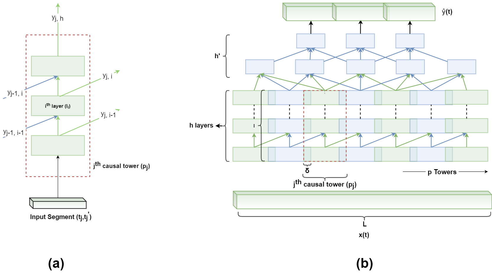
In this paper, we use convolutional neural towers over specified time intervals which perform inter-causal operations. These towers are a set of convolutional layers at different levels as shown in Fig. 1a, which are expected to extract relevant representations from the input sequence and transform it into a more useful space with respect to the objective of the network. For any time interval $(t_{1},t_{2})$, for each layer $l_{i}\forall$ $i\in\{1,2,3,..h\}$, the $j^{th}$ causal tower $p_{j}$ takes input from the tower $p_{j-1}$ in the previous interval, $(t_{0},t_{1})$, such that $t_{0}<t_{1}<t_{2}$ and $t_{1}-t_{0}=t_{2}-t_{1}$. Here, $p$ is the total number of casual towers and $h$ is the number of layers in each of these units. These towers collectively are expected to learn relevant representations from the input sequence which evolve over time. For these towers to instead process the input smoothly, with lesser loss of features in between these time-intervals where corresponding towers are placed, SyncNet uses them as overlapping windows. That is, choose the intervals to place causal towers such that the time-interval of the $j^{th}$ tower, $(t_{j},t^{{}^{\prime}}_{j})$ overlaps with that of the subsequent tower i.e., $(t_{j+1},t^{{}^{\prime}}_{j+1})$ or $t^{{}^{\prime}}_{j}>t_{j+1}$. Let these samples overlapping between each of the intervals be defined as $\delta=t^{{}^{\prime}}_{j}-t_{j+1}$. One may trivially obtain the following relation between all such hyper-parameters of the network.

$$l\approx\frac{L-s}{(1-\gamma)(p-1)}$$ (2)

where $l=t^{{}^{\prime}}_{j}-t_{j}$ is the number of samples in each of the time interval, $L$ is the total number of samples in the input sequence, $\gamma=\delta/l$ is the proportion of overlapping samples in an interval, and $s$ is the number of samples left at the end of the sequence, after a maximum possible integer has been selected for $p$. For the $i^{th}$ layer in the $j^{th}$ tower in this causal structure, the resulting sequence is defined as-

$$y_{j,i}[n] =x_{j,i}^{{}^{\prime}}[n]*h_{j,i}[n]=\sum_{c=0}^{l-1}{x_{j,i}^{{}^{\prime}}[c].h_{j,i}[c+n]}$$

$$=\sum_{c=0}^{l-1}{(y_{j-1,i-1}[c]+y_{j,i-1}[c]).h_{j,i}[c+n]}$$ (3)

Here, $h_{j,i}[n]$ is the filter and $x_{j,i}^{{}^{\prime}}[n]=y_{j-1,i-1}[n]+y_{j,i-1}[n]$ is the input fed causally to the layer at $(j,i)$.

After the input data is passed through the first $h$ levels in this causal structure, our study introduces anti-causal forward passing to deduce emerging relations in the neighborhoods of any interval. With this, the network can leverage to use either set of layers more dominantly, allowing for a much intensive deduction of representations from the input sequence. The architecture of this semi-causal convolutional neural network for 1-D sequences is depicted by Fig. 1b. Any block in this part of the architecture is fed by input from the towers on previous, same and next time-intervals.

Figure 1: SyncNet: A semi-causal convolutional neural network for audio data. (a): Causal Convolution Tower, (b): SyncNet

2.2 Objective Function

The cross-correlation function of two signals $x_{1}(t)$ and $x_{2}(t)$, where $E[.]$ denotes the expectation is defined as-

$$R_{x_{1}x_{2}}(\tau)\overset{def}{=}E[x_{1}(t)x_{2}(t-\tau)]$$ (4)

The argument $\tau=\tau_{0}$ which maximizes $R_{x_{1}x_{2}}(\tau)$ corresponds to the estimate of temporal delay in two signals. Carter et al. [7] and Song et al. [23] showed that using cross-correlation function either directly or upon some filtered variant of the signal results into acceptable performance as a time delay estimator.

Let $\hat{y_{1}}(t)$ and $\hat{y_{2}}(t)$ be the predicted sequences for the input noisy-delayed and reference signals, $x_{1}(t)$ and $x_{2}(t)$ respectively by the network. The cross-correlation function of both sequences can be denoted by $\hat{R}_{y_{1}y_{2}}(\tau)$. The network should learn to transform the input sequences such that $\hat{R}_{y_{1}y_{2}}(\tau)$ peaks at the actual delay in time. The use of cross-correlation function to form a training objective has not been explored before, as far as we know. The closest we know is the concept of maximizing cross-correlation for static features, not time sequences, in the case of deep canonical correlation analysis of multi-modal data [24].

We formulate the loss function as a regression loss. We aim to match the cross correlation sequence to a Gaussian sequence, that peaks at the true time delay. In case of periodic signals, their cross-correlation function will also be periodic, leading us to use a sequence of Gaussians.

$$R(\tau)=\sum_{n=0}^{g-1}{\frac{1}{\sigma_{n}\sqrt{2\pi}}\exp{-\frac{{(\tau-\mu_{n})}^{2}}{2\sigma_{n}^{2}}}}$$ (5)

where $\mu_{n}=T_{0}+nT$ is the $n^{th}$ onset, and $\mu_{0}=T_{0}$ is the actual delay in time and $T$ is the time period of the reference signal (if periodic). For this context and simplicity, we can set $\sigma_{n}=\sigma$ $\forall$ $n\in\{0,1,2,...(g-1)\}$. Let $\mathcal{L}$ be a distance metric between $R(\tau$) and $\hat{R}_{y_{1}y_{2}}(\tau)$. Since the number of peaks are likely to be far lesser in number than other points in the target sequence, we up-weighted $\mathcal{L}$ at $\tau=\tau_{0}+nT$ by $u$ and correspondingly down-weighted for other indices by $d$. The values of these constants are algebraically computed as-

$$d\leftarrow 1-\frac{g+1}{\lambda}\;\;\text{and}\;\;u\leftarrow d+\frac{N^{{}^{\prime}}}{\lambda}$$ (6)

Here, $\lambda=10^{a}$ for the smallest number $a$ such that $\lfloor\frac{N^{{}^{\prime}}}{10^{a}}\rfloor=0$ and $N^{{}^{\prime}}$ is the number of samples in $\hat{R}_{y_{1}y_{2}}(\tau)$. This allows the network to attend to the peaks more likely. We define $\mathcal{L}$ as-

$$\mathcal{L}(.)\overset{def}{=}l_{1}\mathcal{L}_{1}(.)+l_{2}\mathcal{L}_{2}(.)+l_{3}\mathcal{L}_{3}(.)$$ (7)

Here, $\mathcal{L}_{1}=\sum_{i=1}^{N^{{}^{\prime}}}{{(R_{i}-\hat{R}_{i})}^{2}}$ is a simple MSE function, $\mathcal{L}_{2}=\sqrt{\sum_{i=1}^{N^{{}^{\prime}}}{{(\log{R_{i}^{\wp}}-\log{\hat{R}_{i}^{\wp}})}^{2}}}$ is the root-mean-log error function, $\mathcal{L}_{3}=\sum_{i=1}^{N^{{}^{\prime}}}{R_{i}^{\wp}(\log{R_{i}^{\wp}}-\hat{R}_{i}^{\wp})}$ is the KL-Divergence loss and $l_{i}\forall i\in\{1,2,3\}$ are the corresponding weights associated to each term. $R^{p}(\tau)$ and $\hat{R}^{p}(\tau)$ are the pooled correlation sequences, i.e. the most activated for every $p$ set of samples in $R(\tau)$ is chosen as $i^{th}$ sample in $R^{p}(\tau)$. Note that, $\mathcal{L}_{1}$ is applied onto the correlation sequences, thus helps with matching its shape with target, whereas, $\mathcal{L}_{2}$ and $\mathcal{L}_{3}$ are operating over the pooled sequences. One must be cautious while choosing a value for $p$ as a least-bound for the error made by network is expected by nearly $\wp/N^{{}^{\prime}}$. Thus, the estimated parameters, where $\ast$ represents the cross-correlation operation are-

$$\hat{\theta}=\underset{\theta\in\Theta}{min\ }\mathcal{L}(R(\tau),\hat{y}_{1}(t)\ast\hat{y}_{2}(t))$$ (8)

3 Evaluation

3.1 Dataset Used

We evaluate the proposed method on a variety of datasets - including both real recordings as well as synthetically generated audio.

We prepare a new dataset, called MTic. A reference audio signal of periodic tics with a time period of $1$s is played on an phone speaker and is recorded by the microphone of the same phone. Tics are chosen for experiments because they are localized in time and are musically relevant (as in metronome). The recordings are done with a number of phones and in a variety of acoustic background conditions. The time delay in the recorded signal is $<0.9$s. There are total 170 audio recordings sampled at $16kHz$, each of a duration of almost $10$ seconds. They all correspond to the same reference audio of $10$s duration.

Furthermore, to increase the sample size, we synthetically generate 450 audio files from the same reference signal with delays chosen uniformly between $(0s,0.9s]$ and noise injections with signal-to-noise ratio varying in $[-15dB,20dB]$.

To validate the robustness of this study over real world signals such as speech and music as well. We experiment with speech files from the LibriSpeech dataset [25]; speech is non periodic. We also experiment with the accompaniment music from MIREX 2012 dataset [26], which we call MBeats dataset. We randomly sample around 50 audio files from both and generated 25 synthetic audio files for each of these files, with injected delays and noise with SNR randomly sampled from $[-15dB,20dB]$.

The MTic dataset as well as the codes to reproduce the results in this paper are available at https://github.com/madhavlab/2022_syncnet.

3.2 Experiments

We have conducted several experiments to validate the robustness of SyncNet. Both reference and signal-of-interest need to be transformed into embeddings, trained for the task-at-hand. For this, both the signals are parallely passed separately through the same network.

Table 1: Network architecture studied. Here $k$ represents the $k^{th}$ anti-causal layer

Network Part	Layer
	Conv1D + Relu ($h_{1}$ and $h_{3}$)
Causal $\times 1$	Conv1D + BatchNorm1D + Relu ($h_{2}$ and $h_{4}$)
	Conv1D + Relu: ($h_{5}$)
	Conv1D + Relu ($h^{{}^{\prime}}_{k1}$)
Anti-Causal $\times 5$	Conv1D ($h^{{}^{\prime}}_{k2}$)
	BatchNorm1D + Relu ($h^{{}^{\prime}}_{k3}$)

Figure 2: Normalized-Loss for SyncNet during training epochs

Table 2: Hyperparameters for proposed methodology. CT denotes ’Causal Tower/s’ and AC denotes ’Anti-Causal Structure’

Hyperparameter	Description	Value
$l$	Samples per tower	3432
$p$	Number of CT	50
$\gamma$	$\delta/l$	0.125
$h$	Depth of CT	5
$h^{{}^{\prime}}$	Depth of AC	5
$f^{h}_{i}$	Filters in CT	{60,72,54,54,54}
$f^{h^{{}^{\prime}}}_{i}$	Filters in AC	{54,50,32,16,16}
$\eta$	Initial Learning Rate	9e-4

Pooling layers are not used. Batch-Normalization [27] layers are used in between and layers are activated using the ReLU function [28] as in Table 1. It is natural to choose intervals such that the receptive field grows and more samples of the input signal are captured by the causal towers per interval. We have experimented with various values for $p$ with the objective to have lesser samples in $\hat{R}(\tau)$, lesser learnable-parameters and higher receptive field, which led us to set it at $50$. The pool size ($\wp$) has been set as 63. The values for other hyperparameters discussed previously can be realized from table 2. We trained the network on MTic until the losses converge, for a maximum 200 epochs. Mean squared error between the estimated value of delay and the true delay value is chosen as the evaluation metric.

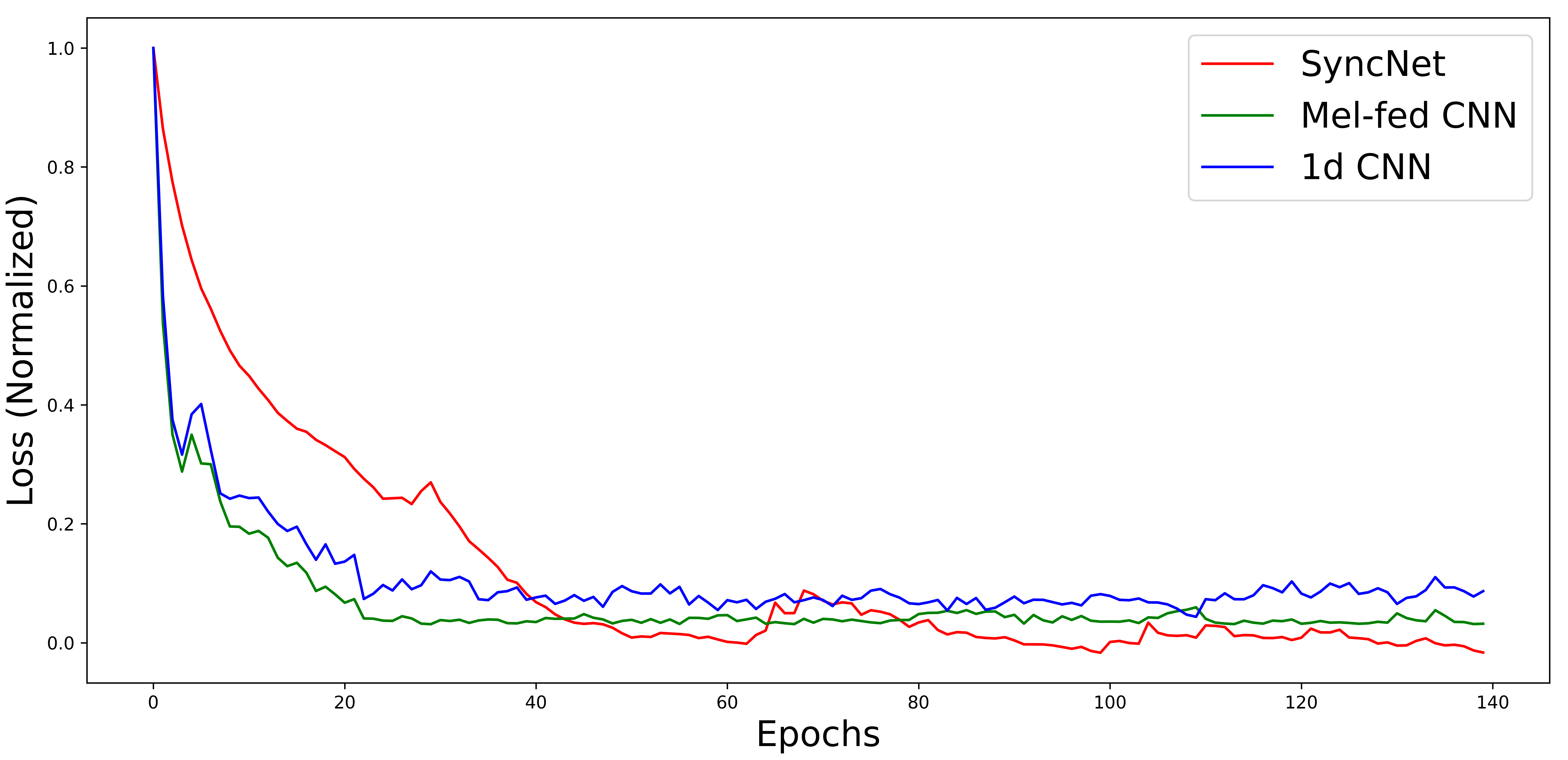
For baseline, we train a deep 1-D audio fed-ConvNet (AfC), a Mel-Spectrogram fed ConvNet (MSfC) with similar layers and Cross-Entropy Loss function. A log of training loss decay for all three networks for first 140 epochs has been plotted in figure 2.

Table 3: Mean squared error in time delay estimation, and the corresponding standard deviation (within brackets), obtained for all the methods on the three datasets

Method	MTic	LibriSpeech	MBeats
Cross-Correlation	0.093(0.091)	0.102(0.098)	0.098(0.095)
GCC-PHAT	0.064(0.077)	0.081(0.069)	0.073(0.082)
AfC	0.071(0.085)	0.091(0.087)	0.066(0.083)
MSfC	0.054(0.082)	0.063(0.075)	0.059(0.086)
SyncNet	0.018(0.075)	0.028(0.072)	0.022(0.083)

Figure 3: Violin plots for absolute error for GCC-PHAT, MfCN and SyncNet on all 3 datasets. Vertically lower distribution indicates better performance.

We compare the performance of the proposed SyncNet based method with four baselines – two neural-networks discussed and the two standard signal processing based methods, namely, the Cross-Correlation method and the classic GCC-PHAT method for time delay estimation.

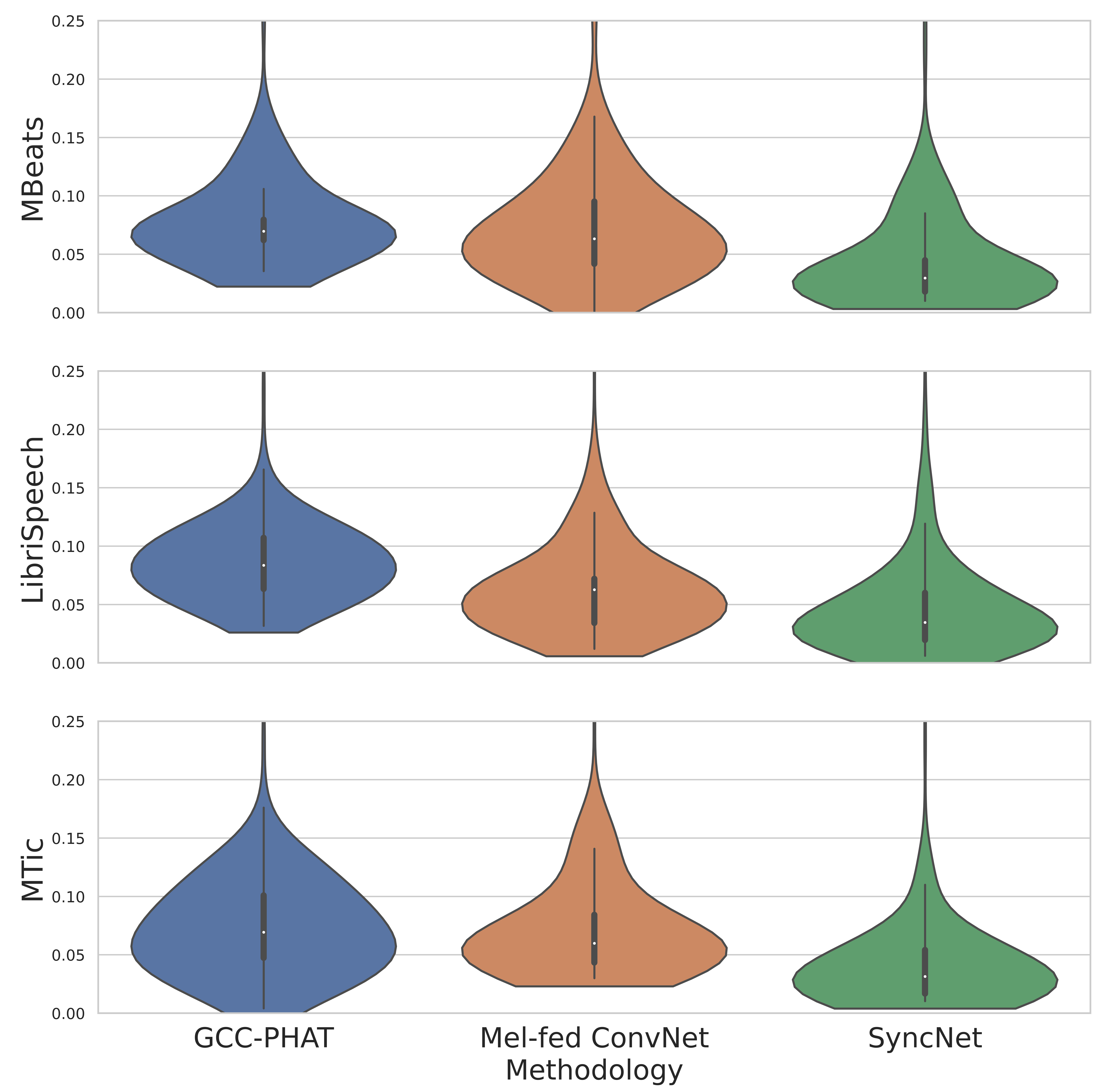
Table 3 shows the mean squared error (MSE) and its standard deviation (SD) for all the methods on the three datasets – MTic, Librispeech and MBeats. We can see that SyncNet consistently outperforms all the baseline methods over all the datasets in terms of the average performance. However, to dive deeper into the performance of the three top performing methods, we draw the violin plots to see the distribution of errors across all test samples. Figure 3 shows these violin plots. It can be seen that the estimation errors for the proposed SyncNet method are distributed more towards the lower end as compared to other methods, supporting the improvements brought in it.

It is important to note that the proposed SyncNet method is not limited by the length of the signals, and performs consistently with signals of variable lengths, maintaining its higher precision. Also, it accepts signals of different sampling rates.

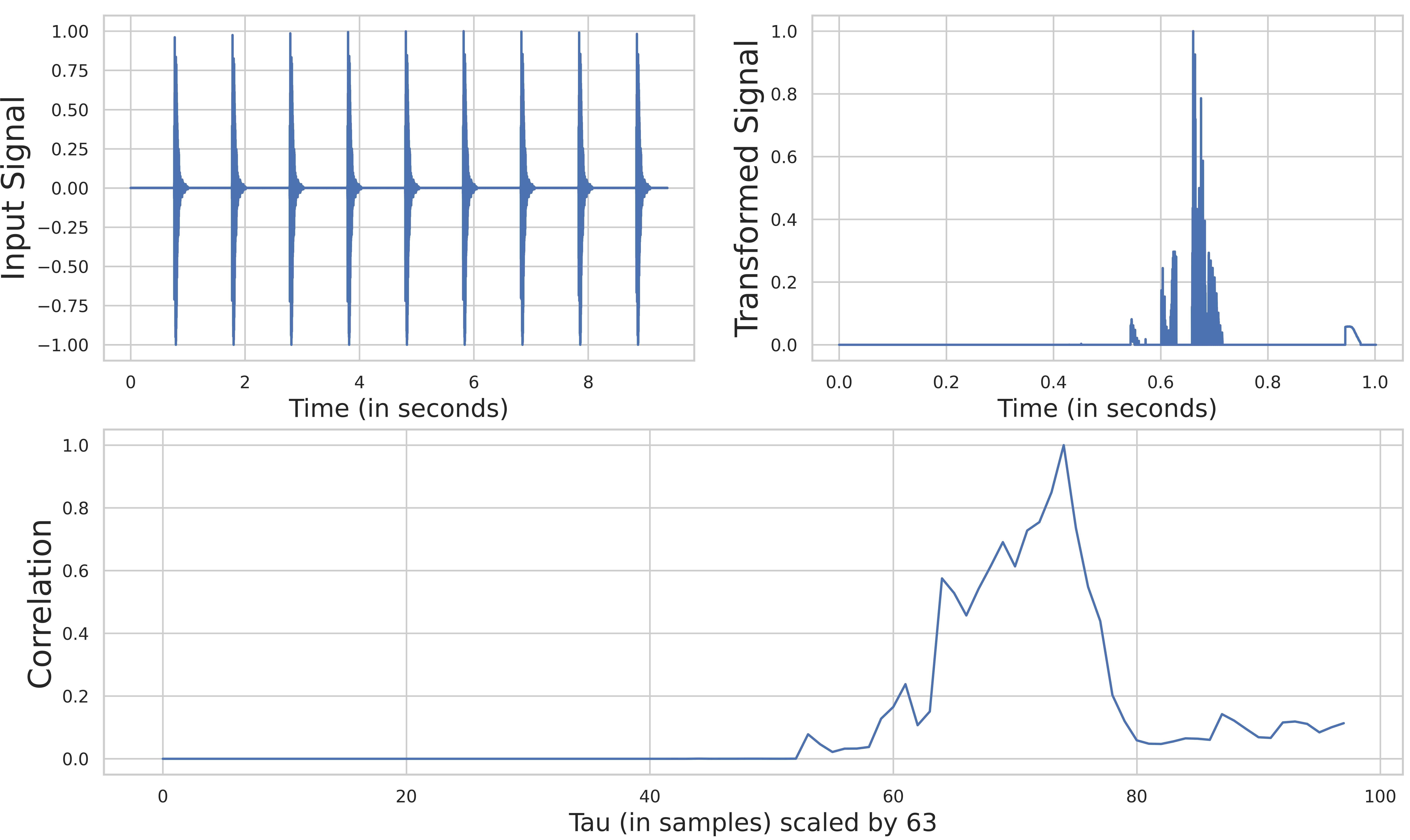
The estimators based on Signal Processing methods [7, 8] are considered more explainable, and thus hold higher potential for fine tuning and debugging [9, 10, 13]. Deep Learning based techniques, on the other hand, mostly lack explainability. Nevertheless, SyncNet transforms a pair of input sequences into a pair of sequences that are correlated to the extent that a simple signal processing metric, such as cross-correlation, can be used to estimate their mutual time delay. This makes the network explainable for its predictions, as one remains informed of the causality of predictions made by the network. As an example, Figure 4 shows a reference signal from MTic database as input to SyncNet, the output of SyncNet and its cross-correlation with that of the corresponding signal-of-interest. A clear peak at the actual delay can be observed in the correlation plot.

Figure 4: Input delayed-noisy signal, its transformed variant and pooled correlation sequence estimated. The correlation peaks correctly at the actual time delay, i.e., 73 samples.

4 Conclusions

We introduce a novel correlation-objective function based deep neural network with causally convolving modules followed by anti-causal convolution sets which enhance the performance of time delay estimation. With optimal choice of hyperparameters, the network also grows its receptive field. SyncNet outperforms all of the classic approaches in precise estimation of time delays. We are working towards applying this method to problems such as round trip latency estimation for audio playback and recording on mobile devices. This synchronized audio can be used by an online service provider to learn the distortion as well as time delay characteristics of these devices in the wild.

5 Acknowledgements

This work was supported by IMPRINT-2C grant from SERB, Government of India, Project no. IMP/2019/400.

References

- [1] C.-H. Park and J.-H. Chang, “Closed-form localization for distributed mimo radar systems using time delay measurements,” IEEE Transactions on Wireless Communications, vol. 15, no. 2, pp. 1480–1490, 2015.
- [2] I. Jameson, Time Delay Estimation, ser. AD-a449 711. Defence Science and Technology Organisation Edinburgh (Australia) Electronic Warfare and Radar Division, 2006.
- [3] J. Schnupp, I. Nelken, and A. King, Auditory neuroscience: Making sense of sound. MIT press, 2011.
- [4] B. Nordlund, “Physical factors in angular localization,” Acta oto-laryngologica, vol. 54, no. 1-6, pp. 75–93, 1962.
- [5] S. Zaporowski, M. Blaszke, and D. Weber, “Measurement of latency in the android audio path,” in Audio Engineering Society Convention 144. Audio Engineering Society, 2018.
- [6] C. Chafe, M. Gurevich, G. Leslie, and S. Tyan, “Effect of time delay on ensemble accuracy,” in Proceedings of the international symposium on musical acoustics, vol. 31. ISMA Nara, 2004, p. 46.
- [7] C. Knapp and G. Carter, “The generalized correlation method for estimation of time delay,” IEEE transactions on acoustics, speech, and signal processing, vol. 24, no. 4, pp. 320–327, 1976.
- [8] K. Scarbrough, N. Ahmed, and G. Carter, “An experimental comparison of the cross correlation and scot techniques for time delay estimation,” in ICASSP’80. IEEE International Conference on Acoustics, Speech, and Signal Processing, vol. 5. IEEE, 1980, pp. 807–810.
- [9] J. Chen, J. Benesty, and Y. Huang, “Time delay estimation in room acoustic environments: An overview,” EURASIP Journal on Advances in Signal Processing, vol. 2006, pp. 1–19, 2006.
- [10] R. Lyon, “A computational model of binaural localization and separation,” in ICASSP’83. IEEE International Conference on Acoustics, Speech, and Signal Processing, vol. 8. IEEE, 1983, pp. 1148–1151.
- [11] Q. Song and X. Ma, “High-resolution time delay estimation algorithms through cross-correlation post-processing,” IEEE Signal Processing Letters, vol. 28, pp. 479–483, 2021.
- [12] M. Cobos, F. Antonacci, L. Comanducci, and A. Sarti, “Frequency-sliding generalized cross-correlation: A sub-band time delay estimation approach,” IEEE/ACM Transactions on Audio, Speech, and Language Processing, vol. 28, pp. 1270–1281, 2020.
- [13] E. Ren, G. C. Ornelas, and H.-A. Loeliger, “Real-time interaural time delay estimation via onset detection,” in ICASSP 2021-2021 IEEE International Conference on Acoustics, Speech and Signal Processing (ICASSP). IEEE, 2021, pp. 4555–4559.
- [14] L. Comanducci, M. Cobos, F. Antonacci, and A. Sarti, “Time difference of arrival estimation from frequency-sliding generalized cross-correlations using convolutional neural networks,” in ICASSP 2020-2020 IEEE International Conference on Acoustics, Speech and Signal Processing (ICASSP). IEEE, 2020, pp. 4945–4949.
- [15] L. Houegnigan, P. Safari, C. Nadeu, M. van der Schaar, M. Solé, and M. André, “High performance supervised time-delay estimation using neural networks,” in IEEE International Conference on Acoustics, Speech and Signal Processing. Proceedings, 2017.
- [16] S. Shaltaf, “Neural-network-based time-delay estimation,” EURASIP Journal on Advances in Signal Processing, vol. 2004, no. 3, pp. 1–8, 2004.
- [17] Q. Li, X. Zhang, and H. Li, “Online direction of arrival estimation based on deep learning,” in 2018 IEEE International Conference on Acoustics, Speech and Signal Processing (ICASSP). IEEE, 2018, pp. 2616–2620.
- [18] h. Li, X. Ziuhhang, and H. Li, “yet to choose,” in 2018 IEEE International Conference on Acoustics, Speech and Signal Processing (ICASSP). IEEE, 2018, pp. 2616–2620.
- [19] S. Chakrabarty and E. A. Habets, “Broadband doa estimation using convolutional neural networks trained with noise signals,” in 2017 IEEE Workshop on Applications of Signal Processing to Audio and Acoustics (WASPAA). IEEE, 2017, pp. 136–140.
- [20] E. Kazakos, A. Nagrani, A. Zisserman, and D. Damen, “Slow-fast auditory streams for audio recognition,” in ICASSP 2021-2021 IEEE International Conference on Acoustics, Speech and Signal Processing (ICASSP). IEEE, 2021, pp. 855–859.
- [21] W. He, P. Motlicek, and J.-M. Odobez, “Multi-task neural network for robust multiple speaker embedding extraction,” Proc. Interspeech 2021, pp. 506–510, 2021.
- [22] A. v. d. Oord, S. Dieleman, H. Zen, K. Simonyan, O. Vinyals, A. Graves, N. Kalchbrenner, A. Senior, and K. Kavukcuoglu, “Wavenet: A generative model for raw audio,” arXiv preprint arXiv:1609.03499, 2016.
- [23] Q. Song and X. Ma, “High-resolution time delay estimation algorithms through cross-correlation post-processing,” IEEE Signal Processing Letters, vol. 28, pp. 479–483, 2021.
- [24] G. Andrew, R. Arora, J. Bilmes, and K. Livescu, “Deep canonical correlation analysis,” in International conference on machine learning. PMLR, 2013, pp. 1247–1255.
- [25] V. Panayotov, G. Chen, D. Povey, and S. Khudanpur, “Librispeech: an asr corpus based on public domain audio books,” in 2015 IEEE international conference on acoustics, speech and signal processing (ICASSP). IEEE, 2015, pp. 5206–5210.
- [26] 2019. [Online]. Available: https://www.music-ir.org/mirex/wiki/2019:Audio_Beat_Tracking
- [27] S. Ioffe and C. Szegedy, “Batch normalization: Accelerating deep network training by reducing internal covariate shift,” in International conference on machine learning. PMLR, 2015, pp. 448–456.
- [28] V. Nair and G. E. Hinton, “Rectified linear units improve restricted boltzmann machines,” in ICML, 2010.