Wormholes with a warped extra dimension?

Abstract

We investigate the role of a specifically warped extra dimension in constructing examples of higher dimensional spacetimes representing Lorentzian wormholes. The warping chosen is largely inspired by the well-known non-static Witten bubble of nothing, though our spacetimes are static and geometrically different. Vacuum solutions in $D\geq 5$ dimensions and others (non-asymptotically flat) with ‘perfectly normal’ matter stress energy are interpreted as possible Lorentzian wormholes. Asymptotically flat wormholes in $D\geq 5$ with ‘exotic matter’ and within this class of spacetimes also appear to exist in all dimensions. A wormhole-black hole correspondence via double Wick rotation is revisited and discussed. Finally, geodesic motion as well as the behaviour of geodesic congruences, in the sub-class of five dimensional, warped, vacuum wormhole spacetimes is also briefly analysed, with the aim of obtaining characteristic properties and specific signatures which may help improve our understanding of these geometries.

I Introduction

The idea of the ‘wormhole’ has its precursors in the work of Flamm flamm on geometry of Schwarzschild spacetime (Flamm’s paraboloid) and, subsequently, in the construction of the Einstein–Rosen bridge erb as a ‘particle model’ in General Relativity (GR). Later, in the late 1950s, Wheeler coined the term ‘wormhole’ while building a topological model of electric charge and working on spacetimes which he christened as geons wheeler . The Bronnikov–Ellis (BE) be ; be2 spacetime of the early 1970s is the first known wormhole solution in General Relativity (GR) albeit with a somewhat absurd, negative kinetic energy scalar field. Nevertheless, the BE spacetime is indeed a ‘solution’. In the 1980s and 1990s, Euclidean and Lorentzian wormholes emerged in two different contexts, the former heralded through the seminal 1988 work of Giddings and Strominger gs and the latter pioneered by Morris and Thorne mt (see also mty ), also in 1988. Since then, wormhole physics has grown into an industry with newer contributions on various issues and questions appearing regularly in the literature (for a recent review from a different perspective, see kundu ).

Let us briefly recall the definition of a Lorentzian wormhole a la Morris–Thorne mt . Assuming a general static, spherically symmetric line element in four dimensions given as

$$ds^{2}=-e^{2\psi(r)}dt^{2}+\frac{dr^{2}}{1-\frac{b(r)}{r}}+r^{2}d\Omega_{2}^{2}$$ (1)

we say that it represents a wormhole if (a) $e^{2\psi(r)}$ has no zeros, i.e. there are no event horizons, (b) $\frac{b(r)}{r}\leq 1$ and $b(r=b_{0})=b_{0}$, i.e. $b_{0}\leq r\leq\infty$ and (c) $\frac{b(r)}{r}$, $\psi(r)$ tend to zero as $r\rightarrow\infty$. The condition $(c)$ guarantees asymptotic flatness while the functional nature of $b(r)$ (obeying the constraints) gives the wormhole shape. Thus, Lorentzian wormholes are horizon-less, asymptotically flat, non-singular spacetimes with their spacelike sections having the shape representing two asymptotically flat regions connected by a bridge. The smallest value of $r$ denoted as $b_{0}$ is named the wormhole throat. The expansion of a geodesic congruence exhibits a defocusing feature as one crosses the throat from one side towards the other asymptotically flat region– this being the basic reason behind the violation of the convergence condition, as envisaged from the Raychaudhuri equation ec .

It is thus a known fact that such static Lorentzian wormhole spacetimes mt cannot exist as solutions in GR with the required matter satisfying the so-called convergence conditions (or, equivalently, in GR, the energy conditions, such as the Null Energy Condition (NEC), the Weak Energy Condition (WEC)) or their averaged versions ec ; visserbook ). Therefore, violating energy conditions is a necessity (for potential counterexamples, see (i) bk where a different class of metrics is used and (ii) radu ,konoplya for scenarios in Einstein-Maxwell-Dirac theory). To address such violations in a constructive sense one either tries to justify it (eg. quantum field theoretic, effective quantum matter stress-energy or arbitrarily small ‘amount’ of energy condition violations) qft ; vkd ; kdv or move away from GR mg ; mg1 ; mg2 ; mg3 ; mg4 . Numerous examples exist in all these approaches. One can indeed have wormholes in modified gravity without violating the energy conditions, as suggested in many articles in the more recent past mgrecent1 ; mgrecent2 .

Another approach to resolve this problem is to introduce/accept the existence of extra dimensions. There have been earlier attempts along these lines zanganeh ,wed , bronnikov ,kuhfittig . Here, we try a different route which we now elaborate on below.

Let us consider a line element of the form:

$$ds^{2}=-e^{2\psi(r)}dt^{2}+\frac{dr^{2}}{1-\frac{b(r)}{r}}+r^{2}d{\Omega_{2}^{2}}+f^{2}(r)d\chi^{2}$$ (2)

where $f(r)$ is the so–called warping function and $\chi$ is the extra dimension which we choose to be angular ($0\leq\chi\leq 2\pi$). The fact that $f$ is a function of $r$ is the reason behind the use of the term ‘warped’. In recent times, the notion of warping has been heavily used in the context of braneworld models rs . There, the idea of a warped braneworld implies the dependence of the four dimensional timelike section of the higher dimensional line element, on the extra dimensional coordinate, usually through a conformal factor. In our line element, as stated above, it is the extra dimensional part of the line element which is assumed to be dependent on one (here $r$) of the so-called ‘four’ dimensional coordinates.

The line element is static and any $\chi=$constant section is spherically symmetric. There are Killing vectors corresponding to the coordinates $t$, $\phi$ and $\chi$ and hence, corresponding constants of motion/conserved quantities. Topologically the manifold is $R^{2}\times S^{2}\times S^{1}$. In other words, $t=$constant, $r=$constant sections are toroidal – somewhat reminiscent of the ‘ringholes’ introduced in gonzalez (see also bronnikov , kuhfittig ). We may further generalise the above line element by introducing a $(D-3)$ sphere instead of a 2-sphere to define a $D$ dimensional line element.

A known, non-static vacuum solution in five dimensions is the Witten bubble line element witten given by

$$ds^{2}=-\alpha^{2}r^{2}dt^{2}+\frac{dr^{2}}{1-\frac{b_{0}^{2}}{r^{2}}}+r^{2}\cosh^{2}\alpha t\,\left(d{\theta^{2}+\sin^{2}\theta d\phi^{2}}\right)+R^{2}\left(1-\frac{b_{0}^{2}}{r^{2}}\right)d\chi^{2}$$ (3)

This line element may be obtained through a double Wick rotation ($\tau\rightarrow i\,R\chi$, $\eta\rightarrow i\alpha t+\frac{\pi}{2}$) of the five dimensional Schwarzschild solution given by

$$ds^{2}=-\left(1-\frac{b_{0}^{2}}{r^{2}}\right)d\tau^{2}+\frac{dr^{2}}{1-\frac{b_{0}^{2}}{r^{2}}}+r^{2}\left(d\eta^{2}+\sin^{2}\eta\,d\theta^{2}+\sin^{2}\eta\sin^{2}\theta d\phi^{2}\right)$$ (4)

A non-vacuum generalisation of the Witten bubble (not obtainable through any Wick rotation) discussed recently in sk21 is given as,

$$ds^{2}=-\alpha^{2}r^{2}dt^{2}+\frac{dr^{2}}{1-\frac{b_{0}^{2}}{r^{2}}}+r^{2}\cosh^{2}\rho_{1}t\,d{\Omega_{2}^{2}}+R^{2}\left(1-\frac{b_{0}^{2}}{r^{2}}\right)d\chi^{2}$$ (5)

where $\alpha\neq\rho_{1}$. If we now set $\rho_{1}=0$, we obtain a static spacetime which can be generalised further by replacing the $\frac{b_{0}^{2}}{r^{2}}$ in $g_{rr}$ and $g_{\chi\chi}$ by $\frac{b(r)}{r}$. We maintain the feature $g_{rr}g_{\chi\chi}=R^{2}$. In other words, the extra dimension disappears near $r=b_{0}$ (the throat of the wormhole), and is maximal as $r\rightarrow\infty$. One can also replace the $-\alpha^{2}r^{2}$ in $g_{00}$ with a generic $g_{00}=-e^{2\psi(r)}$. Later, in the next section, we will work with $\psi=0$.

In summary, what we take from the Witten bubble is the fact that the extra dimension decays away from the asymptotic regions as we move towards the throat. As we shall see, this feature and the specific form of the line element we use helps us in ensuring that the energy conditions hold within the tenets of higher dimensional General Relativity. As mentioned before, our wormhole has $t,r=$constant ($r>b_{0}$) sections which are toroidal (i.e $S^{2}\times S^{1}$ or, more generally, $S^{D-3}\times S^{1}$) with both the radii (of $S^{2}$ or $S^{D-3}$ and $S^{1}$) increasing as we move away from $r=b_{0}$ towards larger values. The $S^{2}$ or $S^{D-3}$ radius is ever-increasing while that of the extra dimensional $S^{1}$ is zero at the throat $r=b_{0}$, increases for $r>b_{0}$ but saturates to a finite constant $R$ as we approach $r\rightarrow\infty$ (see Figure 1). We will now see how the specific form of the warped extra dimension influences the higher dimensional Einstein equations and leads to specific solutions with distinct features.

The rest of this article is organised as follows. In Section II we present the vacuum solutions. Section III discusses the non-vacuum case. Finally, in Section IV geodesics and geodesic congruences are analysed. Our concluding remarks appear in Section V.

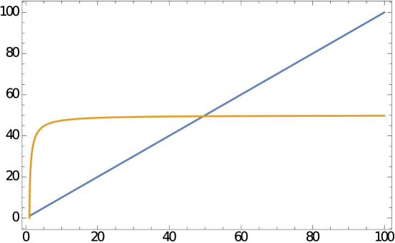
Figure 1: Plot of the radii of the $S^{D-3}$ (blue) and $S^{1}$ (yellow) as a function of the coordinate $r$. Here we have chosen $D=5$, $b(r)=b_{0}$, $b_{0}=1$ and $R=50$ for the line element in (6).

II The vacuum wormhole spacetimes in $D\geq 5$

Following our approach as mentioned in the Introduction, we propose to work with an ultrastatic line element given as:

$$ds^{2}=-dt^{2}+\frac{dr^{2}}{1-\frac{b(r)}{r}}+r^{2}d\Omega_{D-3}^{2}+R^{2}\left(1-\frac{b(r)}{r}\right)d\chi^{2}$$ (6)

The above line element is in $D$ dimensions. $b(r)$ satisfies all requirements typical of a wormhole but is left unspecified for the time being. The previously (in the Introduction) mentioned $\psi(r)$ is set to zero in order to make the geometry ultrastatic. In $D=5$, one can imagine the line element in Eqn. (6) as a four dimensional spacetime with a warped extra dimension ($\chi$). When $D>5$, we adopt the viewpoint of a $D-1$ dimensional spacetime with an extra dimension (the $\chi$). Alternatively, one may choose to think of a $D>5$ scenario as a four dimensional spacetime with $D-4$ extra dimensions.

A curious feature of the $r=b_{0}$ section of the geometry is worth mentioning. The induced four dimensional metric on this section has a determinant equal to zero–hence it is degenerate, but due to the vanishing extra dimension sandipan . However, it is the spatial part (not $g_{tt}$) of the induced metric which leads to its degenerate character. One therefore cannot call $r=b_{0}$ an event horizon (it is not an infinite redshift surface) and there is an ambiguity in referring to it as a null surface according to the standard definition vollick . Nevertheless, to indicate its special character, we will refer to $r=b_{0}$ as a degenerate throat and discuss its characteristics later.

To make further progress, we need to write down the Einstein tensors $G_{ij}$ for the metric in Eqn. (6). Thereafter, assuming $D$ dimensional GR (i.e. $G_{ij}=\kappa T_{ij}$, $\kappa$ related to the $D$ dimensional gravitational constant) we obtain the components of the energy–momentum tensor $T_{00}=\rho$, $T_{11}=\tau$, $T_{jj}=p$ ($j=2,3...D-2$); $T_{D-1\,D-1}=p_{D-1}$, in the frame basis as,

$$\rho=\frac{1}{\kappa}G_{00}=\frac{1}{\kappa}\left[\frac{b^{\prime\prime}}{2r}+(D-4)\left(\frac{2b^{\prime}r+(D-5)b}{2r^{3}}\right)\right],$$ (7)

$$\tau=p_{D-1}=\frac{1}{\kappa}G_{11}=\frac{1}{\kappa}G_{D-1\,D-1}=-(D-3)\left(\frac{b^{\prime}r+(D-5)b}{2r^{3}}\right),$$ (8)

$$p=\frac{1}{\kappa}G_{jj}=\frac{1}{\kappa}\left[-\frac{b^{\prime\prime}}{2r}-(D-5)\left(\frac{(D-6)b+2b^{\prime}r}{2r^{3}}\right)\right],$$ (9)

where, a prime denotes differentiation w.r.t. $r$. The Ricci scalar is given as:

$$R=\frac{b^{\prime\prime}}{r}+(D-4)\left(\frac{2b^{\prime}}{r^{2}}+(D-5)\frac{b}{r^{3}}\right)$$ (10)

and the Kretschmann scalar is:

$$K=2(D-3)\left[\left(\frac{b^{\prime}r-b}{r^{3}}\right)^{2}+(D-4)\frac{b^{2}}{r^{6}}\right]+\frac{\left(b^{\prime\prime}r^{2}-2b^{\prime}r+2b\right)^{2}}{r^{6}}$$ (11)

It is easy to see that a vacuum solution (i.e. $G_{ij}=0$) is given by

$$b(r)=\frac{b_{0}^{D-4}}{r^{D-5}}$$ (12)

One can arrive at the above solution by just solving the $\tau=p_{D-1}=0$ equation–the other two equations ($\rho=0$ and $p=0$) are automatically satisfied by the solution from $\tau=p_{D-1}=0$.

Thus, for $D=5$ we have a line element given as:

$$ds^{2}=-dt^{2}+\frac{dr^{2}}{1-\frac{b_{0}}{r}}+r^{2}d\Omega_{2}^{2}+R^{2}\left(1-\frac{b_{0}}{r}\right)d\chi^{2}$$ (13)

where the $\chi=constant$ section is simply the ultrastatic spatial Schwarzschild wormhole. For this solution, $R=0$ and $K=12\frac{b_{0}^{2}}{r^{6}}$.

It must be stated that this five dimensional vacuum line element was, as far as our knowledge goes, first mentioned in an unpublished preprint by Roberts roberts . Earlier work by Stotyn, Mann stotyn and Miyamoto, Kudoh kudoh on Einstein–Maxwell as well as Einstein-p-form theories were concerned with related non-vacuum solutions. More recently, Bah and Heidmann bah1 , bah2 have explicitly re-mentioned these types of vacuum solutions in five dimensions. However, the notion that these solutions could actually represent Lorentzian wormholes has never been analysed in any detail. Further, consequences for any $b(r)$ vis-a-vis the energy conditions, non-asymptotically flat scenarios, geodesic motion and the behaviour of geodesic congruences have not been dealt with before. Our purpose in this article is to work on these aspects, to some extent.

To provide a $D>5$ example let us now write down the line element in $D=6$. We have,

$$ds^{2}=-dt^{2}+\frac{dr^{2}}{1-\frac{b_{0}^{2}}{r^{2}}}+r^{2}d\Omega_{3}^{2}+R^{2}\left(1-\frac{b_{0}^{2}}{r^{2}}\right)d\chi^{2}$$ (14)

which, for $\chi=constant$, is a Bronnikov-Ellis like spacetime be ; be2 but with a $S^{3}$ instead of a $S^{2}$ and a warped extra dimension. Here $R=0$ and $K=72\frac{b_{0}^{4}}{r^{8}}$. One may construct likewise, examples in other higher dimensions too. Thus, one may state that this entire family of vacuum spacetimes represent Lorentzian wormholes in $D\geq 5$. The solution in $D=4$ (to be considered again later) turns out to be flat spacetime and is not obtainable directly from the general expression provided above for $b(r)$.

Let us then switch to an important issue–the NEC inequalities ec for the matter required to support generic spacetimes with any $b(r)$ satisfying the wormhole criteria. The NEC, for our case, is stated in terms of the two expressions for $\rho+\tau$ and $\rho+p$ (note that $\tau=p_{D-1}$, so $\rho+p_{D-1}$ is not different from $\rho+\tau$). We have,

$$\rho+\tau=\frac{1}{\kappa}\left[\frac{b^{\prime\prime}}{2r}+\frac{(D-5)(b^{\prime}r-b)}{2r^{3}}\right]\geq 0$$ (15)

$$\rho+p=\frac{1}{\kappa}\left[\frac{b^{\prime}r+(D-5)b}{r^{3}}\right]\geq 0$$ (16)

To proceed further, we recall the central result emerging from the Morris-Thorne theorem on wormhole existence and energy conditions mt , in four dimensions. Consider the four dimensional static, spherically symmetric line element stated before in Eqn. (1). A $t=$constant, $\theta=\frac{\pi}{2}$ two dimensional section of this four dimensional line element has an induced metric given as

$$ds^{2}=\frac{dr^{2}}{1-\frac{b(r)}{r}}+r^{2}d\phi^{2}$$ (17)

Embedding this section in three dimensional Euclidean space (cylindrical coordinates) with the line element

$$ds^{2}=dz^{2}+dr^{2}+r^{2}d\phi^{2}$$ (18)

and defining a profile function $z(r)$ we find, from a comparison of the two dimensional line elements (Eqn. (17) and Eqn. (18) with $z=z(r)$),

$$\frac{dz}{dr}=\pm\sqrt{\frac{b}{r-b}}$$ (19)

The requirement on $z(r)$ for a wormhole shape implies that $r(z)$ has a minimum at $z=0$ which corresponds to the smallest value of $r$, i.e. $r=b_{0}$. The minimum ($\frac{d^{2}r}{dz^{2}}(z=0)>0$) is possible only if $b-b^{\prime}r>0$, a result which follows from the expression for $\frac{d^{2}r}{dz^{2}}$, i.e.

$$\frac{d^{2}r}{dz^{2}}=\frac{b-b^{\prime}r}{2b^{2}}.$$ (20)

In contrast, the four dimensional Einstein equations for the metric in Eqn (1) imply, via the Einstein tensor and the energy conditions (assuming the Einstein equation in GR), the NEC relation $\rho+\tau=\frac{1}{\kappa}\left(\frac{b^{\prime}r-b}{r^{3}}\right)\geq 0$ (when $\psi=0$). Hence, we end up with a contradiction which necessitates the violation of the NEC if wormholes have to exist in four dimensional GR with the added assumption that NEC must hold good.

It is easy to see that for the line elements in Eqn. (2) or Eqn. (6), the above analysis (resulting in $b^{\prime}r-b<0$), from the embedding side of the argument, remains unaltered. This happens because the line elements in Eqn. (2) or Eqn. (6) (for say, $D=5$) have $t=$constant, $\theta=\frac{\pi}{2}$ and $\chi=$constant two dimensional sections which are the same as the $t=$constant, $\theta=\frac{\pi}{2}$ two dimensional sections of the line element in Eqn. (1).

Interestingly, the new expressions for the energy condition inequalities (Eqns. (15) and (16)) in the $D$ dimensional spacetimes, do not imply any specific requirement on $b^{\prime}r-b$ for $D\geq 5$. In fact, Eqns. (15) and (16) do lead to restrictions on $b(r)$, but they are not directly on $b^{\prime}r-b$ and therefore different from what is found for the four dimensional line element in Eqn. (1).

Thus, it is possible to have higher dimensional spacetimes representing wormholes and, remarkably, we do end up with vacuum wormholes, for which there is no issue of energy condition violation! It is notable that the warping of the extra dimension in the manner shown in Eqn. (2) or Eqn. (6) plays a major role in this analysis and the ensuing result.

Let us now recall another related class of spacetimes with generic line elements of the form

$$ds^{2}=-\left(1-\frac{b(r)}{r}\right)d\tau^{2}+\frac{dr^{2}}{1-\frac{b(r)}{r}}+r^{2}d\Omega_{D-3}^{2}+R^{2}d\xi^{2}$$ (21)

The line element on a $\xi=$constant slice is spherically symmetric, static and written in the Schwarzschild gauge. The extra, unwarped compact dimension is represented by the coordinate $\xi$. The radius of the extra-dimensional $S^{1}$ is $R$ and it is the same for all $r$, unlike the earlier line element in Eqn. (2) where we had a warped extra dimension. Line elements of the type in (21) fall within the class known as black strings and branes (for a good recent review of past literature see collingbourne , for the specific case of vacuum solutions see roberts , bah1 , bah2 ).

Interestingly, as is well–known bah1 ; bah2 , one can obtain from the above metric, the one given in Eqn. (6) by a double Wick rotation – $\tau\rightarrow i\,R\chi$ and $\xi\rightarrow\frac{i}{R}\,t$. The geometry in Eqn. (21) could be a black hole with an extra dimension depending on the existence of a horizon ($g_{00}(r_{H})=0$) and a singularity inside the horizon. The novelty here is quite straightforward –the horizon, topologically, is not just $S^{D-3}$ but $S^{D-3}\times S^{1}$. The Ricci scalar $R$ and the Kretschmann scalar $K$ for this geometry are the same as given earlier in Eqns. (10) and (11), respectively. Thus, for any $b(r)$, the geometries represented by Eqn. (6) and Eqn (21) have the same Ricci and Kretschmann scalars. However, the Einstein tensor and hence, the energy–momentum tensor components are different (for the non-vacuum cases) and given by:

$$\rho^{BH}=\frac{1}{\kappa}G_{00}=-\tau^{BH}=-\frac{1}{\kappa}G_{11}=\frac{1}{\kappa}\left[(D-3)\left(\frac{b^{\prime}r+(D-5)b}{2r^{3}}\right)\right]$$ (22)

$$p^{BH}=\frac{1}{\kappa}G_{jj}=\frac{1}{\kappa}\left[-\frac{b^{\prime\prime}}{2r}-(D-5)\left(\frac{2b^{\prime}r+(D-6)b}{2r^{3}}\right)\right]$$ (23)

$$p_{D-1}^{BH}=\frac{1}{\kappa}G_{D-1\,D-1}=\frac{1}{\kappa}\left[-\frac{b^{\prime\prime}}{2r}-(D-4)\left(\frac{(D-5)b+2b^{\prime}r}{2r^{3}}\right)\right]$$ (24)

The vacuum solution here, is once again $b(r)=\frac{b_{0}^{D-4}}{r^{D-5}}$ (note that $b_{0}$ here can, in general, be different from the $b_{0}$ in the wormhole). One can obtain this solution by solving the $\rho^{BH}=0$ equation–its solution satisfying the $p^{BH}=0$ and $p_{D-1}^{BH}=0$ equations automatically. The vacuum spacetime with the chosen $b(r)$ represents a black hole with an unwarped compact extra dimension and a toroidal horizon. In $D=5$ it is just a Schwarzschild black hole with a $S^{2}\times S^{1}$ horizon topology. When $D=6$, we end up with a $M=0$, ‘$Q^{2}<0$’ mutated Reissner–Nordström spacetime (recall the Einstein-Rosen bridge! erb ) with a compact extra dimension and a similar toroidal horizon of topology $S^{3}\times S^{1}$. The Wick-rotated counterparts of all these black hole spacetimes are wormholes with toroidal $t,r=$ constant sections (for $r>b_{0}$) and a degenerate throat ($r=b_{0})$. However, the above spacetime in (21) does have a maximal extension and can be continued to the region $r<b_{0}$, i.e. inside the horizon (at $r=b_{0}$), for specific choices of $b(r)$ admitting a horizon (and also a singularity inside the horizon). In contrast, for the wormhole obtained by Wick rotation one must have $r\geq b_{0}$, otherwise, one encounters a signature change and associated pathologies.

An important next question that may arise is – what happens if there is matter? Is it still possible to have wormholes without violating the energy conditions or do we need exotic matter? What kind of black holes (Eqn (21)) do we end up with? We dwell on these queries briefly in the following section.

III Non-vacuum spacetimes in diverse dimensions

Let us first analyse the special case $D=5$. Here we find a rather unusual result for the expressions given for $\rho$, $\tau$, $p$ and $p_{4}$. Writing them down explicitly, we find

$$\rho=\frac{1}{\kappa}\left(\frac{b^{\prime\prime}}{2r}+\frac{b^{\prime}}{r^{2}}\right)$$ (25)

$$\tau=p_{4}=-\frac{1}{\kappa}\frac{b^{\prime}}{r^{2}}$$ (26)

$$p=-\frac{1}{\kappa}\frac{b^{\prime\prime}}{2r}$$ (27)

Notice that only derivatives of $b$ appear. If we now consider the WEC or the NEC, it is easy to see that they will be satisfied as long as $b(r)$ and its first two derivatives are always positive, i.e. $b^{\prime}$ and $b^{\prime\prime}$ are always greater than zero. A standard example could be

$$b(r)=b_{0}^{\nu}r^{1-\nu}\hskip 14.45377pt;\hskip 14.45377ptb^{\prime}(r)=b_{0}^{\nu}(1-\nu)r^{-\nu}\hskip 14.45377pt;\hskip 14.45377ptb^{\prime\prime}(r)=b_{0}^{\nu}\nu(\nu-1)r^{-\nu-1}$$ (28)

where $\nu\leq 0$ if $b$, $b^{\prime}$ and $b^{\prime\prime}$ are to be positive. However, such a choice of $\nu$ does not yield an asymptotically flat spacetime or a wormhole. It is only when $\nu=1$, i.e. vacuum, that we get an asymptotically flat spacetime and a wormhole without any energy condition violations. On the other hand, if we allow violation of the energy conditions we can surely have non-vacuum wormholes for $0\leq\nu\leq 1$.

Beyond $D=5$, a similar result persists. For general $D$ and with the above choice of $b(r)$, the inequalities in Eqns. (15) and (16) lead to the relations $\rightarrow$ $\nu(\nu-D+4)\geq 0$ and $(D-4-\nu)\geq 0$, respectively. For $0\leq\nu\leq 1$ both relations cannot hold simultaneously. In contrast, when $\nu<0$ they lead to a single inequality $(|\nu|+D-4)\geq 0$, which can indeed be satisfied but leads to a non-asymptotically flat spacetime. Thus, it is only the vacuum spacetimes ($\nu=D-4$) mentioned earlier which can have the features of an asymptotically flat Lorentzian wormhole, as long as energy conditions are to be respected with ‘matter’ (here, vacuum) defined via the higher dimensional Einstein field equations. This statemnent is of course restricted to the class of $b(r)$ mentioned above in Eqn. (28). For other choices of $b(r)$ it may be possible to restrict the region over which energy condition violations occur. One can indeed play around with different choices of $b(r)$ and analyse the resulting consequences and differences with the standard four dimensional wormholes.

An interesting case arises when $b(r)=\Lambda r^{3}$ (i.e. $\nu=-2$, $\Lambda=\frac{1}{b_{0}^{2}}$, $D=5$). This yields (using the expressions for $D=5$)

$$\rho=\frac{6\Lambda}{\kappa}\hskip 14.45377pt;\hskip 14.45377pt\tau=p_{4}=-\frac{3\Lambda}{\kappa}\hskip 14.45377pt;\hskip 14.45377ptp=-\frac{3\Lambda}{\kappa}$$ (29)

For $\Lambda>0$, the energy conditions hold and the Ricci scalar $R=12\Lambda$. If we now write a new $b(r)=\Lambda r^{3}+b_{1}$ ( yielding the same values on the R. H. S. in the above equations) we can obtain a non-asymptotically flat Lorentzian wormhole satisfying the energy conditions with its throat radius given by $b_{0}=\sqrt{\frac{\beta-1}{\beta}}\frac{1}{\sqrt{\Lambda}}$ ($\beta>1$) where $b_{0}=\beta b_{1}$. Hence, if we give up asymptotic flatness then there is a possibility of constructing wormholes with normal matter.

Another important question is – what happens for $D=4$ for this class of metrics? To answer this we write down $\rho$, $\tau$ and $p$ in four dimensions.

$$\rho=\frac{1}{\kappa}\left(\frac{b^{\prime\prime}}{2r}\right)$$ (30)

$$\tau=p_{3}=\frac{1}{\kappa}\left(\frac{b-b^{\prime}r}{2r^{3}}\right)$$ (31)

$$p=\frac{1}{\kappa}\left(-\frac{b^{\prime\prime}}{2r}+\frac{b^{\prime}r-b}{r^{3}}\right)$$ (32)

Now the $\rho+p$ inequality requires $b^{\prime}r-b>0$ which contradicts the condition $b-b^{\prime}r>0$, for a wormhole, from the embedding analysis. Thus, in $D=4$, one ends up with NEC violating exotic matter for such wormholes with toroidal ($S^{1}\times S^{1}$) $r>b_{0}$ sections and a degenerate throat, to exist within the framework of GR. Unlike what we found for $D\geq 5$, in $D=4$, for the given class of metrics, giving up asymptotic flatness cannot rescue us from avoiding energy condition violations.

Finally, let us see how the stress-energy ($\rho^{BH}$, $\tau^{BH}$, $p^{BH}$ and $p_{4}^{BH}$) required to support a black hole (Eqn. (21)) are related to that for the wormhole (i.e. $\rho$, $\tau$, $p$, and $p_{4}$). We restrict to $D=5$ and compare Eqns (22), (23), (24) with (7), (8), (9) to get

$$\rho^{BH}=-\tau=\frac{1}{\kappa}\frac{b^{\prime}}{r^{2}}\hskip 14.45377pt;\hskip 14.45377pt\tau^{BH}=\tau=-\frac{1}{\kappa}\frac{b^{\prime}}{r^{2}}$$ (33)

$$p^{BH}=p=-\frac{1}{\kappa}\frac{b^{\prime\prime}}{2r}\hskip 14.45377pt,\hskip 14.45377ptp_{4}^{BH}=-\rho=\frac{1}{\kappa}\left(-\frac{b^{\prime\prime}}{2r}-\frac{b^{\prime}}{r^{2}}\right)$$ (34)

Thus, for the wormhole, as we noted earlier, energy conditions will hold if $b^{\prime}>0$, $b^{\prime\prime}>0$. In contrast, for the black hole, we require $b^{\prime\prime}<0$ and $b^{\prime\prime}<\frac{2b^{\prime}}{r}$. For example when $b(r)=2M-\frac{Q^{2}}{r}$ we obtain a Reissner-Nordström black hole (with an extra dimension) with matter satisfying the energy conditions. With the same $b(r)$, the wormhole geometry is generated with NEC violating matter. In general, $\rho^{BH}+\tau^{BH}=0$ but $\rho^{BH}+p^{BH}=p-\tau$ and $\rho^{BH}+p_{4}^{BH}=-\left(\rho+\tau\right)$. Hence we have the following intriguing result: a NEC violating wormhole ($\rho+\tau<0$ but $p\geq\tau$) could correspond to a NEC satisfying black hole ($\rho^{BH}+\tau^{BH}\geq 0$ as well as $\rho^{BH}+p^{BH},p_{4}^{BH}\geq 0$) for the same $b(r)$!

In order to further appreciate and unravel specific characteristics of these spacetimes in $D\geq 5$, let us now focus on particle trajectories.

IV Geodesics

Among many possible studies which can be done in any new spacetime, knowing about geodesic motion is perhaps a first. We will study geodesics in the five dimensional vacuum geometry where $b(r)=b_{0}$. The geodesic Lagrangian is given as:

$${\cal L}=-{\dot{t}}^{2}+\frac{{\dot{r}}^{2}}{1-\frac{b_{0}}{r}}+r^{2}{\dot{\theta}}^{2}+r^{2}\sin^{2}\theta{\dot{\phi}}^{2}+R^{2}\left(1-\frac{b_{0}}{r}\right){\dot{\chi}}^{2}=-k$$ (35)

where $k=1$ (timelike) or $k=0$ (null). From the first integrals for $t$, $\phi$ and $\chi$ we obtain,

$$\dot{t}=E\hskip 14.45377pt;\hskip 14.45377pt\dot{\phi}=\frac{L}{r^{2}}\hskip 14.45377pt;\hskip 14.45377pt\dot{\chi}=\frac{C}{R^{2}\left(1-\frac{b_{0}}{r}\right)}$$ (36)

where we have chosen $\theta=\frac{\pi}{2}$ without any loss of generality. $E$, $C$ and $L$ are the constants of motion. In particular, $C$ is associated with the extra dimension $\chi$.

Using the above expressions, it is easy to find $\dot{r}$, which is given as,

$$\dot{r}=\pm\sqrt{\left(E^{2}-k-\frac{L^{2}}{r^{2}}\right)\left(1-\frac{b_{0}}{r}\right)-\frac{C^{2}}{R^{2}}}$$ (37)

and hence, an effective ‘potential’ is

$$V_{eff}(r)=-\frac{1}{2}\left(E^{2}-k-\frac{L^{2}}{r^{2}}\right)\left(1-\frac{b_{0}}{r}\right)+\frac{C^{2}}{2R^{2}}$$ (38)

Note that ${\dot{r}}^{2}=-V_{eff}(r)$ and hence, $r$ values where $V_{eff}\leq 0$ correspond to regions where physical motion is allowed.

For $L=0$ it is possible to obtain $t(r)$ in terms of simple functions though the expression is not invertible. We find, after integrating,

$$t=\sqrt{\frac{r(\alpha r-\beta)}{\alpha^{2}}}+\frac{\beta}{\alpha^{\frac{3}{2}}}{\sinh}^{-1}\sqrt{\frac{\alpha r-\beta}{\beta}}$$ (39)

where $\alpha=1-\frac{k}{E^{2}}-\frac{C^{2}}{E^{2}R^{2}}$ and $\beta=b_{0}\left(1-\frac{k}{E^{2}}\right)$. Note that $t=0$ at $r=\frac{\beta}{\alpha}<b_{0}$, as long as $C\neq 0$. Thus, the presence of the extra dimension is reflected in the fact that trajectories may not quite reach the wormhole throat unless $C=0$. This could be thought of as a signature of the presence of the extra dimension. Figure 1 shows the solution for $t(r)$ in the left panel for $C\neq 0$ and $C=0$. The corresponding effective potentials are shown on the right panel. One notices the point where $V_{eff}$ is zero and then the region where it is negative which, together reflect the feature just mentioned above.

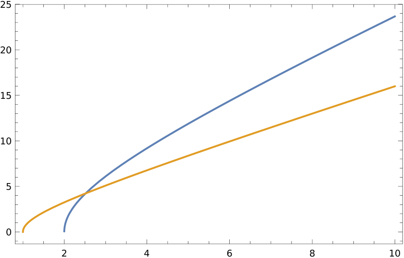
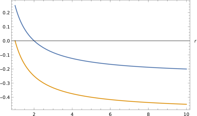
Figure 2: The plots refer to the solution $t(r)$ in (39) and the $V_{eff}$ in (38). Left: $t$ ($y$-axis) vs. $r$ (x-axis) for $k=1,b_{0}=1,E^{2}=2,C^{2}=0.5,R^{2}=1,L=0$ [blue] and $k=1,b_{0}=1,E^{2}=2,C^{2}=0,L=0$ (yellow); Right: $V_{eff}(r)$ ($y$ axis) vs $r$ ($x$ axis) for $k=1,b_{0}=1,E^{2}=2,C^{2}=0.5,R^{2}=1,L=0$ [blue] and $k=1,b_{0}=1,E^{2}=2,C^{2}=0,L=0$ (yellow)

When $L\neq 0$, the solution for $t(r)$, though obtainable, is quite complicated. In order to understand what are the consequences for $L\neq 0$, it is useful to look at $\left(\frac{dr}{dt}\right)^{2}$ which we rewrite below.

$$\left(\frac{dr}{dt}\right)^{2}=\frac{\alpha}{r^{3}}\left[r^{2}(r-\gamma b_{0})-\eta(r-b_{0})\right]$$ (40)

Here $\gamma=\frac{E^{2}-k}{\alpha E^{2}}>1$ and $\eta=\frac{L^{2}}{E^{2}\alpha}$. When $C=0$ we have $\gamma=1$ and any test particle can start out from or reach $r=b_{0}$, as long as $\eta\geq b_{0}^{2}$ (or $L^{2}>\alpha b_{0}^{2}$). When $C\neq 0$ along with $L\neq 0$ we can see that $r=b_{0}$ is not reachable–a result similar to what we found in the $L=0$ case. Hence, in our class of metrics, the inaccessibility of the throat at $r=b_{0}$ seems an unavoidable signature of the presence of extra dimensions. The difference in the asymptotic value of the effective potential for the $C=0$ and $C\neq 0$ cases as well as the presence of the extra dimension in the asymptotic region are both responsible for the above-mentioned behaviour of test particles.

It is also possible to arrive at the above mentioned conclusion by looking at the expansion ($\Theta$) of a timelike geodesic congruence. To understand this better, we rewrite the general line element in the form:

$$ds^{2}=-dt^{2}+dl^{2}+r^{2}(l)d\Omega_{2}^{2}+R^{2}{r^{\prime}}^{2}(l)d\chi^{2}$$ (41)

using the proper radial distance $l(r)$ obtained from

$$\frac{dl}{dr}=\pm\frac{1}{\sqrt{1-\frac{b_{0}}{r}}}$$ (42)

The inverse of $l(r)$ is $r(l)$ and $r^{\prime}(l)=\frac{dr}{dl}$. The normalised timelike geodesic vector field $u^{i}$ is therefore given as:

$$u^{i}\equiv=\left(u^{t},u^{l},u^{\theta},u^{\phi},u^{\chi}\right)\equiv\left(E,\pm\sqrt{E^{2}-1-\frac{L^{2}}{r^{2}}-\frac{C^{2}}{R^{2}{r^{\prime}}^{2}}},0,\frac{L}{r^{2}},\frac{C}{R^{2}{r^{\prime}}^{2}}\right)$$ (43)

where $\theta=\frac{\pi}{2}$ and $r(l)$ is left unspecified though we assume, as before, its wormhole features. The expansion $\Theta$ of a timelike geodesic congruence, i.e. $\Theta=\nabla_{i}u^{i}$ turns out to be:

$$\Theta(l)=\frac{1}{u^{l}}\left(\frac{r^{\prime}}{r}\left\{2(E^{2}-1)-\frac{L^{2}}{r^{2}}-2\frac{C^{2}}{R^{2}{r^{\prime}}^{2}}\right\}+\frac{r^{\prime\prime}}{r^{\prime}}\left\{E^{2}-1-\frac{L^{2}}{r^{2}}\right\}\right)$$ (44)

For $L,C=0$, the expansion takes the simpler form

$$\Theta(l)=\sqrt{E^{2}-1}\left(2\frac{r^{\prime}}{r}+\frac{r^{\prime\prime}}{r^{\prime}}\right)$$ (45)

where the second term is due to the warped extra dimension. One notices that For $L,C=0$, the caustic in $\Theta$ (locus of points where $\Theta\rightarrow-\infty$) arises at the location ($l$ value) where $r^{\prime}(l)=0$, which is the location of the throat. However, when $C\neq 0$, the caustic location shifts away from $l=0$, a fact derivable from the zero value of the denominator factor $u^{l}$ in Eqn. (44). In a four dimensional ultrastatic wormhole spacetime the expansion will just involve $\frac{r^{\prime}}{r}$ and hence there will be defocusing near the throat and no caustic formation. Further, if instead of the line element in (41), we write (21) using the $l$ coordinate, we have

$$ds^{2}=-{r^{\prime}}^{2}(l)dt^{2}+dl^{2}+r^{2}(l)\left(d\theta^{2}+\sin^{2}\theta d\phi^{2}\right)+R^{2}d\xi^{2}$$ (46)

It can be shown that the expansion $\Theta$ of the timelike geodesic congruence will not diverge at the horizon at $l=0$ – in fact it will be finite and negative for any $r(l)$ (or $b(r)$) which satisfies wormhole-like features.

One may therefore, identify the presence of the extra dimension through the location of the caustic. For null geodesics, a parallel analysis can also be done with qualitatively similar consequences.

On the other hand, one may obtain circular orbits by solving $V_{eff}(r_{0})=0$ (i.e. zero radial velocity or $\frac{dr}{dt}=0$) which gives

$$\left(\frac{r_{0}-b_{0}}{r_{0}}\right)\left(\frac{r_{0}^{2}(E^{2}-k)-L^{2}}{r_{0}^{2}}\right)=\frac{C^{2}}{R^{2}}$$ (47)

Notice that $r_{0}=b_{0}$ only when $C=0$. When $C\neq 0$ one has to solve a general cubic equation for $L\neq 0$. We note that there are timelike and null orbits, i.e. for $k=1$ as well as $k=0$. The cubic equation in $\frac{1}{r_{0}}$ can be reduced to a depressed cubic in the variable $y$ by using the transformation $\frac{1}{r_{0}}=y+\frac{1}{3b_{0}}$. We get

$$y^{3}+sy+q=0$$ (48)

where

$$s=-\frac{1}{3b_{0}^{2}}-\frac{E^{2}-k}{L^{2}}=-\frac{1}{3b_{0}^{2}}-\frac{1}{{L^{\prime}}^{2}}$$ (49)

$$q=\frac{1}{L^{\prime 2}b_{0}}\left[\frac{2}{3}-\frac{2{L^{\prime}}^{2}}{27b_{0}^{2}}-d_{0}^{2}\right]$$ (50)

with ${L^{\prime}}^{2}=\frac{L^{2}}{E^{2}-k}$ and $d_{0}^{2}=\frac{C^{2}}{R^{2}(E^{2}-k)}$. It is easy to see that $r_{0}=3b_{0}$ (i.e. $y=0$) is a solution when $L^{\prime 2}=b_{0}^{2}$ and $d_{0}^{2}==\frac{16}{27}$. A general solution can also be written down using the trigonometric method of finding the roots of a cubic.

When $L=0$, expectedly, the analysis is easier. The solution for $r_{0}$ is simple and given as:

$$r_{0}=\frac{b_{0}}{1-\frac{C^{2}}{R^{2}(E^{2}-k)}}$$ (51)

which equals $b_{0}$ for $C=0$ and is always greater than $b_{0}$ as long as $C^{2}<R^{2}(E^{2}-k)$. Choosing $k=1$ or $k=0$ one can find results for timelike and null circular orbits. It is important to note the condition that the circular orbit at $r_{0}$ is a closed curve on the torus defined by $\phi$ and $\chi$ (recall $\theta=\frac{\pi}{2}$). Since we have,

$$\dot{\phi}=\frac{L}{r_{0}^{2}}\hskip 14.45377pt;\hskip 14.45377pt\dot{\chi}=\frac{C}{R^{2}\left(1-\frac{b_{0}}{r_{0}}\right)}$$ (52)

and, therefore,

$$\phi=\frac{L}{r_{0}^{2}}\frac{R^{2}\left(1-\frac{b_{0}}{r_{0}}\right)}{C}\chi$$ (53)

The closure of the curve is dependent on the requirement

$$\frac{L}{r_{0}^{2}}\frac{R^{2}\left(1-\frac{b_{0}}{r_{0}}\right)}{C}=1$$ (54)

For example, if $r_{0}=3b_{0}$ one ends up with the condition that $\frac{R^{2}}{b_{0}^{2}}=\frac{27}{2}\frac{C}{L}$, which constrains the asymptotic radius of the extra dimension in terms of the wormhole throat. In principle, one may replace the R.H.S. in Eqn. (48) by an integer ‘$n$’ which will imply multiple windings along one direction as equivalent to a single winding along the other.

In summary, one may have three types of closed curves on the ‘torus’ (assuming $\theta=\frac{\pi}{2}$) with coordinates defined by $\phi$ and $\chi$. Constants of motion related to $\phi$ and $\chi$ are $L$ and $C$, respectively. When $L=0$, the closed curves are defined by $\chi$ with $C\neq 0$ for $r_{0}>b_{0}$ (strictly). If $C=0$, similar closed curves are defined via $\phi$ with $L\neq 0$ and with $r_{0}\geq b_{0}$. In general, one may have closed curves with both $L$ and $C$ nonzero for $r>b_{0}$ and with a constraint involving $L$, $C$ and $r_{0}$ which is required for closure. The distinct character of the closed curves for $C\neq 0$ is a signature of the presence of the extra dimension $\chi$.

V Conclusions

To conclude, we summarise our results with comments.

Firstly, we have looked at a class of higher dimensional warped line elements in which, the spacelike section has wormhole features with toroidal $r>b_{0}$ sections and a degenerate throat. For example, in $D=5$, the $r>b_{0}$ sections are, topologically, $S^{2}\times S^{1}$. The nature of the warping (inspired by the Witten bubble geometry) is such that in $D=5$, the extra dimension is maximal in the asymptotic region and has a zero radius at the throat (degenerate throat). Such a higher dimensional wormhole spacetime is shown to exist in vacuum which means that there is no issue with energy conditions or their violation. For $D>5$, the $D-1$ dimensional timelike section represents a higher dimensional wormhole with an additional compact extra dimension. We have written down the general $D$ dimensional vacuum line element. We also show how a black hole line element with a unwarped extra dimension (a black string) can be arrived at using a double Wick rotation of the wormhole metric–thereby revisiting a known correspondence bah1 ; bah2 , with the ‘wormhole’ aspect added. In a broader sense, the two types of spacetimes, i.e. wormholes and black holes seem to exist for different sets of values of parameters in a complex line element of the form

$$ds^{2}=-\left(1-\frac{b(r)}{r}\right)a^{2}e^{2i\alpha}d\tau^{2}+\frac{dr^{2}}{1-\frac{b(r)}{r}}+r^{2}d\Omega_{D-3}^{2}+R^{2}d^{2}e^{2i\beta}d\chi^{2}.$$ (55)

Choosing the pairs $(a,\alpha)$ and $(d,\beta)$ one can obtain the wormhole and the black hole line elements and also write down the double Wick rotations involved in relating the metrics.

A further extension of this link between black holes (black strings) and wormholes is also possible. One can relate wormholes of different types–for example, ultrastatic ones (zero gravitational redshift) with non-ultrastatic ones (finite gravitational redshift). Details along these directions will be discussed in future sk2022 .

Switching over to similar metrics with matter, we find non-asymptotically flat spacetimes which represent a wormhole with an extra dimension without any exotic matter. We also delineate the conditions under which any black hole or wormhole (represented by our class of metrics) could exist, with energy-condition conserving/violating matter. Numerous examples are presented.

Finally, we analyse the geodesics in the $D=5$ vacuum wormhole line element and show how the presence of an extra dimension is manifest in the trajectories of test particles. Importantly, we have, through an analysis of the expansion of a timelike geodesic congruence, shown that the throat is a benign caustic when the geodesics have a constant $\chi$ (extra dimensional coordinate). For a varying $\chi$ this caustic shifts to values larger than the throat radius but is still present.

In a sense, we have found a way to evade the Morris-Thorne theorem by exploiting a warped higher dimensional spacetime which leads to vacuum wormholes or non-asymptotically flat ones with matter. One may argue that these wormholes are not ‘true, traversable wormholes’ because they admit geodesic congruences which end at a benign caustic. In fact, the appearance of the caustic is the precise reason why they exist without violating the convergence or, equivalently for GR, the energy conditions.

An important issue related to both the wormhole and the black hole spacetimes with warped and unwarped extra dimensions respectively, concerns perturbations and stability. It is known that the black string is unstable–a result famously known as the Gregory–Laflamme instability gl1 , gl2 , gl3 , collingbourne . What happens for the wormholes with a warped extra dimension? Further, for both the wormholes and their Wick–rotated counterparts, what happens for different choices of $b(r)$? In particular, to answer these questions one would have to do a detailed study of scalar as well as gravitational perturbations. It is quite likely that such studies can lead to interesting new results for both types of spacetimes for varied choices of $b(r)$.

Going further, it is very much possible to generalise the results here by (a) using different functions (different $b(r)$) in $g_{rr}$ and $g_{\chi\chi}$ (b) removing ultrastaticity by incorporating $e^{2\psi(r)}$ in $g_{tt}$. One may thereby expect more flexibility in constructing astrophysically (and perhaps observationally!) useful, asymptotically flat wormholes and it is likely that energy-condition violations for matter stress-energy may eventually be avoidable, with the caveat that extra/higher dimensions are indeed around!

References

- (1) L. Flamm, Die Grundlagen der Allgemeinen Relativitätstheorie, Ann. d. Phys. 49, 769 (1916).
- (2) A. Einstein and N. Rosen, Phys. Rev. 48, 73 (1935).
- (3) C.W. Misner and J. A. Wheeler, Ann. Phys. 2, 525 (1957).
- (4) K. A. Bronnikov, Acta Phy. Pol. B4, 251 (1973).
- (5) H. Ellis, J. Math. Phys. 14, 104 (1973).
- (6) S. Giddings and A. Strominger, Nucl. Phys. B 306, 890 (1988).
- (7) M. S. Morris and K. S. Thorne, Am. J. Phys.56, 395 (1988).
- (8) M. S. Morris, K. S. Thorne and U. Yurtsever, Phys. Rev. Letts. 61, 1446 (1988).
- (9) A. Kundu, Wormholes and holography, an introduction, arXiv:2110.14958.
- (10) R. M. Wald, General Relativity, The University of Chicago Press, USA, 1984.
- (11) M. Visser, Lorentzian Wormholes: from Einstein to Hawking, AIP Press, Woodbury, NY, 1995.
- (12) K. A. Bronnikov and V. G. Krechet, Phys. Rev. D 99, 084051 (2019).
- (13) J. Blazquez-Salcedo, C. Knoll, E. Radu, Phys. Rev. Lett. 126, 101102 (2021).
- (14) R. Konoplya and A. Zhidenko, Phys. Rev. Lett. 128, 091104 (2022).
- (15) H. Epstein, E. Glaser and A. Yaffe, Nuovo Cimento 36, 1016 (1965).
- (16) M. Visser, S. Kar and N. Dadhich, Phys. Rev. Letts. 90, 201102 (2003).
- (17) S. Kar, N. Dadhich and M. Visser, Pramana 63, 859 (2004).
- (18) T. Harko, F.S.N. Lobo, M. K. Mak, S.V. Sushkov, Phys. Rev. 87, 067504 (2013).
- (19) K. A. Bronnikov and A. M. Galiakhmetov, Grav. Cosmo. 21, 283 (2015).
- (20) M. Hohmann, Phys. Rev. D 89, 087503 (2014).
- (21) R. Shaikh, Phys. Rev. D 92, 024015 (2015).
- (22) R. Myrzakulov, L. Sebastiani, S. Vagnozzi, S. Zerbini, Class. Quant. Grav. 33, 125005 (2016).
- (23) R. Shaikh, Phys. Rev. D 98, 064033 (2018).
- (24) G. Antoniou, A. Bakopoulos, P. Kanti, B. Kleihaus, and J. Kunz, Phys. Rev. D 101, 024033 (2020).
- (25) M. K. Zanganeh, F. S. N. Lobo, M. H. Dehghani, Phys. Rev. D 92, 12409 (2015).
- (26) S. Kar, S. Lahiri and S. SenGupta, Phys. Letts. B 750, 319 (2015).
- (27) K. A. Bronnikov, M. V. Skvortsova, Grav. Cosmo. 22, 316 (2016).
- (28) P. K. F. Kuhfittig, Phys. Rev. D 98, 064041 (2018).
- (29) P. Gonzalez-Diaz, Phys. Rev. D 54, 6122 (1996).
- (30) L. Randall and R. Sundrum, Phys. Rev. Letts. 83, 4690 (1999).
- (31) E. Witten, Nucl. Phys. B 195, 481 (1982).
- (32) S. Kar, Phys. Rev. D 105, 024213 (2022).
- (33) S. Sengupta, Phys. Rev. D 101, 104040 (2020).
- (34) D. Vollick, Eur. Phys. Jr. Plus 130, 157 (2015).
- (35) M. D. Roberts, arxiv: 0901.2307 (gr-qc), unpublished.
- (36) S. Stotyn and R. B. Mann, Phys. Letts. B 705, 269 (2011).
- (37) U. Miyamoto and H. Kudoh, JHEP 12, 048 (2006).
- (38) I. Bah and P. Heidmann, Phys. Rev. Letts. 126, 151101 (2021).
- (39) I. Bah and P. Heidmann, JHEP 09, 147 (2021).
- (40) S. Collingbourne, J. Math. Phys. 62, 032502 (2021) and references therein.
- (41) S. Kar, work in progress.
- (42) R. Gregory and R. Laflamme, Phys.Rev. Lett. 70, 2837 (1993).
- (43) R. Gregory and R. Laflamme, Nucl. Phys. B 428, 399 (1994).
- (44) R. Gregory, The Gregory-Laflamme instability, chapter in Black holes in higher dimensions ed. G. Horowitz, Cambridge University Press, Cambridge, UK (2012), arxiv:1107.5821