Translation Consistent Semi-supervised Segmentation for 3D Medical Images

Abstract

3D medical image segmentation methods have been successful, but their dependence on large amounts of voxel-level annotated data is a disadvantage that needs to be addressed given the high cost to obtain such annotation. Semi-supervised learning (SSL) solves this issue by training models with a large unlabelled and a small labelled dataset. The most successful SSL approaches are based on consistency learning that minimises the distance between model responses obtained from perturbed views of the unlabelled data. These perturbations usually keep the spatial input context between views fairly consistent, which may cause the model to learn segmentation patterns from the spatial input contexts instead of the foreground objects. In this paper, we introduce the Translation Consistent Co-training (TraCoCo) which is a consistency learning SSL method that perturbs the input data views by varying their spatial input context, allowing the model to learn segmentation patterns from foreground objects. Furthermore, we propose the replacement of the commonly used mean squared error (MSE) semi-supervised loss by a new Confident Regional Cross entropy (CRC) loss, which improves training convergence and keeps the robustness to co-training pseudo-labelling mistakes. We also extend CutMix augmentation to 3D SSL to further improve generalisation. Our TraCoCo shows state-of-the-art results for the Left Atrium (LA), Pancreas-CT (Pancreas), and Brain Tumor Segmentation (BRaTS19) datasets with different backbones. Our code, training logs and checkpoints are available at https://github.com/yyliu01/TraCoCo.

1 Introduction

The training of 3D medical image segmentation neural network methods requires large sets of voxel-wise annotated samples. These sets are obtained using a laborious and expensive slice-by-slice annotation process, so alternative methods based on small labelled set training methods have been sought. One example is semi-supervised learning (SSL) that relies on a large unlabelled set and a small labelled set to train the model, and a particularly effective SSL approach is based on the consistency learning that minimises the distance between model responses obtained from different views of the unlabelled data [34, 7].

The different views of consistency learning methods can be obtained via data augmentation [1] or from the outputs of differently initialized networks [38, 7, 15]. Mean teacher (MT) [38, 51, 11, 40, 24] combines these two perturbations and averages the network parameters during training, yielding reliable pseudo labels for the unlabelled data. Various schemes in 3D medical image segmentation are introduced to improve the generalisation of teacher-student methods, including uncertainty guided threshold [51, 11] or multi-task assistance [40, 28]. However, the domain-specific transfer [1] of the teacher-student scheme can cause both networks to converge to a similar local minimum, reducing the network perturbation effectiveness. Moreover, some hard medical segmentation cases are consistently segmented similarly by the teacher and student models, potentially resulting in confirmation bias during training. This issue motivated the introduction of the co-training framework that involves two models that are initialized with different parameters and mutually supervise each other by generating pseudo-labels for the unlabelled data during the training phase. Those two independent models have less chance of converging to the same local minima than the teacher-student model. Recent approaches [7, 15] show that co-training provides an effective consistency regularization with the cross-supervision between two independent networks.

Even though successful, the approaches above can inadvertently learn the segmentation pattern from the spatial input context of the training data rather than from the foreground objects to be segmented, which can yield unsatisfactory pseudo labels for the unlabelled data. For instance, models can memorise segmentation characteristics from background patterns, leading to consistent predictions even when incoming data exhibit variations. This issue is more pronounced in 3D medical data, where the smaller amount of training samples combined with the larger input data dimensionality can increase the dependence between the spatial input context and segmentation results, resulting in poor generalization.  Lai et al. [19] extract intermediate embeddings via a multi-layer perceptron (MLP) and impose consistency constraints on different input contexts through contrastive learning. However, such implicit constraints are unsatisfactory for 3D medical images because of potentially mistaken prediction and the absence of network perturbations (we show results about this in Sec.4.4), which are essential improve the model’s generalisation capability. In fact, we argue that network perturbation combined with a perturbation of the spatial input context to form different views of unlabelled samples is important to reduce the dependence between spatial input context and segmentation predictions.

In this paper, we propose the Translation Consistent Co-training (TraCoCo) algorithm. TraCoCo enforces the segmentation agreement inside the intersection region between translated views of the input data, where an additional log-likelihood regularization is applied to balance the importance of the segmented visual object and the background voxels. For the semi-supervised consistency loss, we propose the Confident Regional Binary Cross-Entropy (CRC) to constrain the cross-model predictions based on the learning of the regions that the model predicts as positive, and of the regions that the model predicts as negative  [17, 3, 36], with the goal of improving training convergence while maintaining the robustness to pseudo-labelling mistakes. Moreover, CutMix [52] has demonstrated significant generalization improvements for 2D data, when the annotated training set is small [7], so we introduce CutMix for the 3D medical data. In summary, we list our contributions below:

1. A novel co-training strategy based on translation consistency that is designed to promote cross-model prediction consistency under spatial input context variation of the input data (see Fig. 1);

2. A new entropy-based CRC loss that takes only the most confident positive and negative pseudo labels to co-train the two models with the goal of improving training convergence and keeping the robustness to pseudo-labelling mistakes;

Our approach yields SOTA results for the semi-supervised benchmarks of the Left Atrium (LA) [48], Pancreas-CT (Pancreas) [9] and BRaTS19 [31], demonstrating its effectiveness and generalisability.

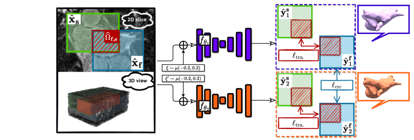
Fig. 1: TraCoCo’s learning with unlabelled data. The input volume $\mathbf{x}$ is randomly cropped into sub-volumes $\hat{\mathbf{x}}_{\mathbf{f}}$ in blue (extracted from image lattice $\widehat{\Omega}_{\mathbf{f}}$) and the translated volume $\hat{\mathbf{x}}_{\mathbf{s}}$ in green (extracted from image lattice $\widehat{\Omega}_{\mathbf{s}}$), where these sub-volumes have a non-empty intersection denoted by the lattice $\widehat{\Omega}_{\mathbf{f,s}}=\widehat{\Omega}_{\mathbf{f}}\cap\widehat{\Omega}_{\mathbf{s}}\neq\emptyset$, represented in red. This pair of sub-volumes are perturbed with uniform noise $\xi$ before being used to produce the segmentation results {$\hat{\mathbf{y}}_{1}^{\mathbf{f}}$, $\hat{\mathbf{y}}_{1}^{\mathbf{s}}$}, {$\hat{\mathbf{y}}_{2}^{\mathbf{f}}$, $\hat{\mathbf{y}}_{2}^{\mathbf{s}}$} from the networks $f_{\theta_{1}}(.)$ and $f_{\theta_{2}}(.)$, respectively. The translation consistency loss $\ell_{\text{tra}}(.)$ in (3) will penalise differences in the responses within $\widehat{\Omega}_{\mathbf{f,s}}$, and the outputs $\hat{\mathbf{y}}_{1}^{\mathbf{f}}$, $\hat{\mathbf{y}}_{2}^{\mathbf{f}}$ are used to minimize $\ell_{crc}(.)$ in (7). On the right-hand side, we show the 3D segmentations produced by the models (purple and orange volumes).

2 Related work

2.1 Semi-supervised Learning

Semi-supervised learning leverages limited labelled data and many unlabelled data to boost the models’ performance. Consistency learning is the dominant idea for semi-supervised learning, consisting of a method that enforces that neighbouring feature representations must share the same labels (i.e., smoothness assumption). The $\Pi$ model [20] proposes the weak-strong augmentation scheme, where the pseudo labels are produced via weakly augmented data and predictions are from its strong augmentation version (i.e., noise perturbation or colour-jittering). To improve pseudo labels’ stability, the $\Pi$ model variant TemporalEmbedding [20] proposes an exponential moving average (EMA) method to accumulate all the historical results. Even though TemporalEmbedding improved stability, the hardware costs of storing the historical results are expensive. Mean Teacher (MT) [38], the most popular semi-supervised structure in current research, solves such issues by ensembling the network parameters to a ”teacher” network via EMA transfer to generate pseudo labels. The main drawback of those consistency-learning methods is that the ensemble of models/predictions eventually fall to the same local minimum during the training [1], where teacher and student models will have the same behaviour for many complex data patterns. In this work, we adopt the Co-training framework [2] that incorporates two different models to produce pseudo labels for unlabelled data and supervise each other simultaneously. Those two models share the same architecture, but their parameters are differently initialised, which brings more diversity when analysing complex input data patterns from challenging medical image segmentation tasks.

2.2 Semantic Segmentation

Fully convolutional network (FCN) [26] is a fundamental model that introduced an efficient dense prediction scheme. Unlike the image segmentation of natural images that relies on large receptive fields [4, 5, 50] or attention [23, 12], the segmentation of medical images is more effective using reconstruction models, primarily represented by the encoder-decoder architecture [33]. The most influential segmentation model for medical images is the UNet [37] that comprises a contracting path to extract the context features and an upsampling path to precisely localise those patterns. The encoder features from the contracting path are concatenated with the decoder features from the upsampling path to avoid the loss of information. Its variant, UNet++ [55] increases convolutional layers and concatenates more peer features to further boost performance. In MRI or CT medical image segmentation,  Çiçek et al. [8] propose the 3D-Unet architecture based on 3D convolution to capture volume patterns more effectively. VNet [32] is a relevant architecture that shares similar properties with 3D-Unet, but with more parameters and convolution layers. In our experiments, we examine our proposed TraCoCo algorithm with the VNet [32] architecture for both LA and Pancreas datasets to ensure fair comparisons with previous works [51, 28]. We also examine the effectiveness of our TraCoCo using the 3D-UNet [8] for the BraTS19 dataset.

2.3 Semi-supervised Medical Image Segmentation

Semi-supervised medical segmentation has received much attention in recent years, where most papers focus on estimating uncertain regions within pseudo labels. Yu et al. [51], Wang et al. [40], Xia et al. [46] propose uncertainty-aware mechanisms that estimate the uncertainty regions for the pseudo labels via Monte Carlo dropout. Luo et al. [27, 29] learn the unsupervised samples progressively via prediction confidence or the distance between the predictions from different scales. Wang et al. [42] estimate the uncertainty via a threshold-based entropy map. Mehrtash et al. [30], Xu et al. [49], Xiang et al. [47] measure uncertainty by the calibration of multiple networks’ predictions. While exploring unlabelled data, these approaches aim to avoid the negative impact of trying to learn from potentially noisy regions. However, by doing that, they have inadvertently neglected the learning of potentially correct pseudo-labels, resulting in insufficient convergence, particularly when dealing with complex input data patterns. This issue has been partly handled by Ishida et al. [14], who proposed a complementary learning method to train from the inverse label information based on negative entropy. Kim et al. [17, 18], Rizve et al. [36] successfully explore negative and positive learning techniques to achieve a good balance between avoiding the learning from potentially noisy regions and mitigating the insufficient convergence issue. In our paper, we address both issues of learning from noisy regions and insufficient convergence with weighted negative and positive learning method that restricts its attention to regions of high classification confidence for foreground and background objects.

To achieve good generalisation, some papers [54, 21, 41] utilise adversarial learning, and others [24, 34, 45, 44] rely on a perturbation across multiple networks to improve consistency. Despite their success in recognising unlabelled patterns, these papers have overlooked the significance of in-context perturbations in input data, which are essential for encouraging the model to differentiate spatial patterns. Lai et al. [19] have proposed a contrastive learning framework to address such spatial information for urban driving scenes’ segmentation. However, their contrastive learning framework depends on potentially mistaken segmentation predictions, which can lead to confirmation bias in the pixel-wise positive/negative sampling strategy, resulting in sub-optimal accuracy when dealing with complex medical images. Also, their framework does not explore network perturbations, which reduces its generalisation ability. In contrast, our TraCoCo successfully promotes cross-model prediction consistency under spatial input context variation, enabling our method to yield promising results across 2D and 3D medical image segmentation benchmarks.

3 Method

For the 3D semi-supervised semantic segmentation, we have a small labelled set $\mathcal{D}_{L}=\{(\mathbf{x},\mathbf{y})_{i}\}_{i=1}^{|\mathcal{D}_{L}|}$, where $\mathbf{x}\in\mathcal{X}\subset\mathbb{R}^{H\times W\times C}$ represents the input volume with size $H\times W$ and $C$ slices, and $\mathbf{y}\in\mathcal{Y}\subset\{0,1\}^{H\times W\times C}$ denotes a binary (foreground vs background) segmentation ground truth. We also have a large unlabelled set $\mathcal{D}_{U}=\{\mathbf{x}_{i}\}_{i=1}^{|\mathcal{D}_{U}|}$ , where $|\mathcal{D}_{L}|<<|\mathcal{D}_{U}|$.

As depicted in Fig. 1, our approach is a co-training framework [35] that contains two differently initialised networks. Both segmentation models work with an input sub-volume $\widehat{\mathcal{X}}\subset\mathbb{R}^{\widehat{H}\times\widehat{W}\times\widehat{C}}$, where $\widehat{H}<H$, $\widehat{W}<W$, and $\widehat{C}<C$. These sub-volumes are extracted from the original volume lattice $\Omega$ using the sub-lattice $\widehat{\Omega}_{\mathbf{f}}\subset\Omega$ of size $\widehat{H}\times\widehat{W}\times\widehat{C}$ and centred at volume index $\mathbf{f}\in\mathbb{N}^{3}$. This sub-volume extracted from volume $\mathbf{x}$ is represented by $\hat{\mathbf{x}}_{\mathbf{f}}=\mathbf{x}(\widehat{\Omega}_{\mathbf{f}})$. The models are represented by $f_{\theta}:\widehat{\mathcal{X}}\to[0,1]^{\widehat{H}\times\widehat{W}\times\widehat{C}}$, where $\theta_{1},\theta_{2}\in\Theta\subset\mathbb{R}^{P}$ denote the $P-$dimensional parameters of the two models.

3.1 Translation Consistent Co-training (TraCoCo)

The proposed translation consistent co-training (TraCoCo) optimisation is based on the following loss function minimization:

$$\theta^{*}_{1},\theta^{*}_{2}=\arg\underset{\theta_{1},\theta_{2}}{\min}\>\>\ell_{sup}(\mathcal{D}_{L},\theta_{1},\theta_{2})+\lambda\Big{(}\ell_{sem}(\mathcal{D}_{U},\theta_{1},\theta_{2})+\ell_{tra}(\mathcal{D}_{L}\cup\mathcal{D}_{U},\theta_{1},\theta_{2})\Big{)},$$ (1)

where the supervised learning loss is defined by

$$\ell_{sup}(\mathcal{D}_{L},\theta_{1},\theta_{2})=\sum_{(\mathbf{x},\mathbf{y})\in\mathcal{D}_{L}}\ell_{ce}(\mathbf{y}^{\mathbf{f}},\hat{\mathbf{y}}^{\mathbf{f}}_{1})+\ell_{ce}(\mathbf{y}^{\mathbf{f}},\hat{\mathbf{y}}^{\mathbf{f}}_{2})+\ell_{dice}(\mathbf{y}^{\mathbf{f}},\hat{\mathbf{y}}^{\mathbf{f}}_{1})+\ell_{dice}(\mathbf{y}^{\mathbf{f}},\hat{\mathbf{y}}^{\mathbf{f}}_{2}),$$ (2)

with $\ell_{ce}(.)$ denoting the voxel-wise cross-entropy loss, $\ell_{dice}(.)$ representing the volume-wise linearised Dice loss [51], $\hat{\mathbf{y}}_{1}^{\mathbf{f}}=f_{\theta_{1}}(\hat{\mathbf{x}}_{\mathbf{f}}+\xi)$ (similarly for $\hat{\mathbf{y}}_{2}^{\mathbf{f}}$, with $\xi\sim\mu(-0.2,0.2)$ denoting a sample from a uniform distribution in the range $[-0.2,0.2]$), and $\mathbf{y}^{\mathbf{f}}=\mathbf{y}(\widehat{\Omega}_{\mathbf{f}})$ representing the sub-volume label. Also in (1), $\ell_{sem}(.)$, defined below in (6), represents the semi-supervised loss that uses the pseudo labels from the two models, $\ell_{tra}(.)$, defined below in (3), denotes the translation consistency loss which enforces the cross-model consistency between the segmentation of two randomly-cropped sub-regions (containing varying spatial input contexts) of the original volume, and $\lambda$ in (1) is a cosine ramp-up function that controls the trade-off between the losses.

3.1.1 Translation Consistency Loss

We take the training volume $\mathbf{x}\in\mathcal{D}_{L}\cup\mathcal{D}_{U}$, and extract two sub-volumes centred at $\mathbf{f},\mathbf{s}\in\mathbb{N}^{3}$, with $\mathbf{f}\neq\mathbf{s}$ and denoted by $\hat{\mathbf{x}}_{\mathbf{f}}$ and $\hat{\mathbf{x}}_{\mathbf{s}}$, where their respective lattices have a non-empty intersection, i.e., $\widehat{\Omega}_{\mathbf{f,s}}=\widehat{\Omega}_{\mathbf{f}}\cap\widehat{\Omega}_{\mathbf{s}}\neq\emptyset$. Our proposed translation consistency loss from (1) is defined by

$$\ell_{tra}(\mathcal{D}_{L}\cup\mathcal{D}_{U},\theta_{1},\theta_{2})=\sum_{\begin{subarray}{c}\mathbf{x}\in\mathcal{D}_{L}\cup\mathcal{D}_{U}\\ \mathbf{f,s}\sim\mathcal{U}(\Omega)\end{subarray}}\alpha\ell_{kl}(\mathbf{x}(\widehat{\Omega}_{\mathbf{f,s}}),\theta_{1},\theta_{2})+\beta\ell_{reg}(\mathbf{x}(\widehat{\Omega}_{\mathbf{f,s}}),\theta_{1},\theta_{2}),$$ (3)

where the centres of the two sub-volumes denoted by $\mathbf{f,s}$ are uniformly sampled from the original volume lattice $\Omega$, $\alpha$ and $\beta$ are hyper-parameters to balance the two loss functions ($\alpha=1.$ and $\beta=0.1$ in the experiments),

$$\ell_{kl}(\mathbf{x}(\widehat{\Omega}_{\mathbf{f,s}}),\theta_{1},\theta_{2})=\sum_{\omega\in\widehat{\Omega}_{\mathbf{f},\mathbf{s}}}\mathbb{KL}(\hat{\mathbf{y}}_{1}^{\mathbf{f}}(\omega),\hat{\mathbf{y}}_{1}^{\mathbf{s}}(\omega))+\mathbb{KL}(\hat{\mathbf{y}}_{2}^{\mathbf{f}}(\omega),\hat{\mathbf{y}}_{2}^{\mathbf{s}}(\omega))$$ (4)

computes the Kullback-Leibler (KL) divergence between the segmentation outputs of the two models in the intersection region of two translated input sub-volumes represented by $\widehat{\Omega}_{\mathbf{f},\mathbf{s}}$, and $\hat{\mathbf{y}}_{1}^{\mathbf{f}}$, $\hat{\mathbf{y}}_{1}^{\mathbf{s}}$, $\hat{\mathbf{y}}_{2}^{\mathbf{f}}$, and $\hat{\mathbf{y}}_{2}^{\mathbf{s}}$ are defined in (2). Also in (3), we have

$$\ell_{reg}(\mathbf{x}(\widehat{\Omega}_{\mathbf{f,s}}),\theta_{1},\theta_{2})=-\sum_{\omega\in\widehat{\Omega}_{\mathbf{f},\mathbf{s}}}\mathbb{H}(\hat{\mathbf{y}}_{1}^{\mathbf{f}}(\omega))+\mathbb{H}(\hat{\mathbf{y}}_{2}^{\mathbf{f}}(\omega))+\mathbb{H}(\hat{\mathbf{y}}_{1}^{\mathbf{s}}(\omega))+\mathbb{H}(\hat{\mathbf{y}}_{2}^{\mathbf{s}}(\omega))$$ (5)

that aims to balance the foreground and background classes in the training voxels, where $\mathbb{H}(.)$ represents Shannon’s entropy.

3.1.2 Confident Regional Cross-Entropy (CRC) Loss

The semi-supervised loss $\ell_{sem}(.)$ in (1) enforces the consistency between the segmentation results by the two models, as follows:

$$\ell_{sem}(\mathcal{D}_{U},\theta_{1},\theta_{2})=-\sum_{\mathbf{x}\in\mathcal{D}_{U}}\sum_{\omega\in\widehat{\Omega}_{\mathbf{f}}}\ell_{crc}\left(\hat{\mathbf{y}}_{1}^{\mathbf{f}}(\omega),\hat{\mathbf{y}}_{2}^{\mathbf{f}}(\omega)\right)+\ell_{crc}\left(\hat{\mathbf{y}}_{2}^{\mathbf{f}}(\omega),\hat{\mathbf{y}}_{1}^{\mathbf{f}}(\omega)\right),$$ (6)

where $\hat{\mathbf{y}}_{1}^{\mathbf{f}}(\omega)\in[0,1]^{2}$ represents the background ($\hat{\mathbf{y}}_{1}^{\mathbf{f}}(\omega)[0]$) and foreground ($\hat{\mathbf{y}}_{1}^{\mathbf{f}}(\omega)[1]$) segmentation probabilities in voxel $\omega\in\widehat{\Omega}_{\mathbf{f}}$ obtained from the softmax activation function of model $1$ (similarly for model $2$),

$$\ell_{crc}(\mathbf{a},\mathbf{b})=\mathbb{I}(\mathbf{a}>\gamma)\times\ell_{ce}(\mathsf{OneHot}(\mathbf{a}),\mathbf{b})+\mathbb{I}(\mathbf{a}<\beta)\times\ell_{ce}(1-\mathsf{OneHot}(\mathbf{a}),1-\mathbf{b})),$$ (7)

with $\mathbb{I}(\mathbf{a}>\gamma)=\begin{cases}\max(\mathbf{a})\hskip 5.69046pt\text{, if }\max(\mathbf{a})>\gamma\\ 0\hskip 5.69046pt\hskip 24.18501pt\text{, otherwise }\end{cases}$, $\mathbb{I}(\mathbf{a}<\beta)=\begin{cases}1-\min(\mathbf{a})\hskip 5.69046pt\text{, if }\min(\mathbf{a})<\beta\\ 0\hskip 5.69046pt\hskip 38.41139pt\text{, otherwise }\end{cases}$, $\mathbf{a},\mathbf{b}$ being a probability distribution of the foreground and background classes of voxel $\omega$, and $\gamma,\beta$ representing hyper-parameters to balance the foreground and background losses. Note that our proposed $\ell_{crc}(.)$ replaces the more common MSE loss [51, 21, 11, 40, 22, 45, 44] used in semi-supervised learning methods, where our goal is to maintain the MSE robustness to the pseudo-label mistakes and improve training convergence. Particularly, in (7), we select confidently classified foreground and background voxels by the first model to train both the positive and negative cross-entropy loss for the second model, and vice-versa.

3.2 3D CutMix

To improve training generalisation using the semi-supervised loss in (6), we extend CutMix [10, 7] from 2D to 3D data. This is achieved by randomly generating a 3D binary mask $\mathbf{m}\in\{0,1\}^{H\times W\times C}$ to a pair of volumes with $\nu^{\mathbf{m}}_{ij}=(1-\mathbf{m})\odot\mathbf{x}_{i}+\mathbf{m}\odot\mathbf{x}_{j}$, where the prediction is obtained with $f_{\theta}(\nu^{\mathbf{m}}_{ij}(\widehat{\Omega}_{\mathbf{f}})+\xi)$. The pseudo labels from the second model is defined by $\hat{\mathbf{y}}^{\mathbf{f}}_{2,ij}=(1-\mathbf{m})\odot\hat{\mathbf{y}}^{\mathbf{f}}_{2,i}+\mathbf{m}\odot\hat{\mathbf{y}}^{\mathbf{f}}_{2,j}$, with $\hat{\mathbf{y}}^{\mathbf{f}}_{2,i}=f_{\theta_{2}}(\hat{\mathbf{x}}^{\mathbf{f}}_{i}+\xi^{\prime})$ and $\hat{\mathbf{y}}^{\mathbf{f}}_{2,j}=f_{\theta_{2}}(\hat{\mathbf{x}}^{\mathbf{f}}_{j}+\xi^{\prime})$. To account for the 3D CutMix, the semi-supervised loss in (6) is re-defined with

$$\ell_{sem}(\mathcal{D}_{U},\theta_{1},\theta_{2})=\sum_{\mathbf{x}_{i},\mathbf{x}_{j}\in\mathcal{D}_{U}}\sum_{\omega\in\widehat{\Omega}_{\mathbf{f}}}\ell_{crc}\left(f_{\theta_{1}}(\nu^{\mathbf{m}}_{ij}(\omega)+\xi),\hat{\mathbf{y}}_{2,ij}^{\mathbf{f}}(\omega)\right)+\ell_{crc}\left(f_{\theta_{2}}(\nu^{\mathbf{m}}_{ij}(\omega)+\xi),\hat{\mathbf{y}}_{1,ij}^{\mathbf{f}}(\omega)\right).$$ (8)

4 Experiments

4.1 Datasets

In order to evaluate the effectiveness of our approach, we conduct experiments on the following publicly available 3D medical image datasets: the Left Atrium (LA) [48], Pancreas-CT (Pancreas) [9], and Brain Tumor Segmentation 2019 (BraTS19) [31]. The LA dataset [48] is from the Atrial Segmentation Challenge that contains $100$ 3D MRI volumes with an isotropic resolution of 0.625 × 0.625 × 0.625 mm. Following previous papers [51, 21], we crop at the centre of the heart region in the pre-processing stage and use 80 volumes for training and 20 for testing (we use the same training and testing sample IDs as in [51, 21]). The Pancreas dataset [9] consists of 82 3D contrast-enhanced CT scans collected from $53$ male and $27$ female subjects at the National Institutes of Health Clinical Center. Each slice in the dataset has a resolution of 512 x 512, but the thickness ranges from 1.5 to 2.5 mm. In the pre-processing stage, we followed the approaches proposed in [44, 28] by clipping voxel values into the range of [-125, 275] Hounsfield Units and re-sampling the data to an isotropic resolution of 1.0 x 1.0 x 1.0 mm. For our experiments, we used 62 samples for training and 20 samples for testing, following the same split sample IDs in [44] for fair comparisons. The BRaTS19 dataset [31] is from the Brain Tumor Segmentation Challenge and contains $335$ brain MRIs with tumour segmentation labels. Each sample in the dataset consists of four MRI scans of the brain: T1-weighted (T1), T1-weighted with contrast enhancement (T1-ce), T2-weighted (T2), and T2 fluid-attenuated inversion recovery (FLAIR). The resolution of each scan is 240 x 240 x 155, and they have been aligned into the same space (1.0 x 1.0 x 1.0 mm). For pre-processing, we follow the approach described in [6] and use only the FLAIR sequences to simplify the task to binary classification. Similar to [51], we centre crop each volume in BRaTS19 with random offsets. In the experiments, we use $250$ volumes for training, $25$ volumes for validation and $60$ for testing.

The LA and Pancreas datasets are commonly used benchmarks for testing semi-supervised 3D medical segmentation methods, so the results from competing methods are from the original papers. In the case of the BraTS19 dataset, the results of the current state-of-the-art (SOTAs) methods are based on our re-implementation.

4.2 Implementation Details

Following [51, 28], we employ VNet [32] for the experiments in the LA and Pancreas datasets, and we utilise 3D-UNet [8] for the BRaTS19 dataset, following [6]. We set the initial learning rate to be $5e^{-2}$, and decay via the poly learning rate scheduler $\left(1-\frac{\text{iter}}{\text{max\_iter}}\right)^{0.9}$, where the max_iter is $15,000$ in LA and Pancreas datasets and $30,000$ in BraTS19 dataset. To balance the supervised and unsupervised losses in (1), we utilize Cosine ramp-up function with $40$ iterations, starting with $\lambda=0$. We adopt mini-batch SGD with momentum to train our model, where the momentum is fixed at $0.9$, and weight decay is set to $0.0005$. In training, each batch consists of $2$ voxel-wise labelled and $2$ unlabelled volumes, and they are cropped to be $112\times 112\times 80$ on LA, and $96\times 96\times 96$ on BraTS19 and Pancreas. We employ the same online augmentation with random crop and flipping following [51, 21]. The semi-supervised learning experimental setup partitions the original training set with 10% and 20% labelled samples and the rest of samples remain unlabelled.

Hardware Requirements. We use one NVIDIA GeForce RTX 3090 GPU to implement our algorithm for the LA dataset, and one 32GB V100 for the BraTS19 and Pancreas datasets because of the larger input volume.

4.3 Evaluation Details

Inference. During testing, we only use one network (i.e., $f_{\theta_{1}}(.)$) to produce our results. The final segmentation is obtained via the sliding window strategy, where the strides are 18x18x4 for the LA dataset, and 16x16x16 for the Pancreas and BraTS19 datasets, following previous works [51, 21, 28, 45, 44]. We report last epoch results in Pancreas and BraTS19 datasets and the best evaluation and last epoch results for the LA datasets.

Measurements. We use four measures to quantitatively evaluate our method, which are Dice, Jaccard, the average surface distance (ASD), and the 95% Hausdorff Distance (95HD). The Dice and Jaccard are measured in percentage, while ASD and 95HD are measured in voxels. Additionally, we measure complexity with the number of model parameters and multiply-accumulate (MAC) during the inference [44].

4.4 Comparison with SOTA approaches

Table 1: Evaluation on the Left Atrium dataset using VNet architecture based on the partition protocols of $8$ and $16$ labelled data. The column best denotes the best checkpoint evaluation protocol and complexity is measured during the inference phase following [44]. Our results are highlighted in cyan, with the best results shown in bold.

Left Atrium	best	# scan used		measures				complexity
		labelled	unlabelled	Dice(%)	Jaccard(%)	ASD(Voxel)	95HD(Voxel)	Param.(M)	Macs(G)
UA-MT [51]	✗	8	72	86.28	76.11	4.63	18.71	9.44	47.02
SASSNet [21]	✗	8	72	85.22	75.09	2.89	11.18	9.44	47.05
LG-ER [11]	✗	8	72	85.54	75.12	3.77	13.29	9.44	47.02
DUWM [43]	✗	8	72	85.91	75.75	3.31	12.67	9.44	47.02
URPC [29]	✗	8	72	85.01	74.36	3.96	15.37	5.88	69.43
CAC [19]	✗	8	72	87.61	78.76	2.93	9.65	9.44	47.02
PS-MT [24]	✗	8	72	88.73	79.02	2.79	8.11	9.44	47.02
TraCoCo (ours)	✗	8	72	89.29	80.82	2.28	6.92	9.44	47.02
DTC [28]	✓	8	72	87.51	78.17	2.36	8.23	9.44	47.05
MC-Net [45]	✓	8	72	87.50	77.98	2.30	11.28	12.35	95.15
MC-Net+ [44]	✓	8	72	88.96	80.25	1.86	7.93	9.44	47.02
TraCoCo (ours)	✓	8	72	89.86	81.70	2.01	6.81	9.44	47.02
UA-MT [51]	✗	16	64	88.74	79.94	2.32	8.39	9.44	47.02
SASSNet [21]	✗	16	64	89.16	80.60	2.26	8.95	9.44	47.05
LG-ER [11]	✗	16	64	89.62	81.31	2.06	7.16	9.44	47.02
DUWM [43]	✗	16	64	89.65	81.35	2.03	7.04	9.44	47.02
URPC [29]	✗	16	64	88.74	79.93	3.66	12.73	5.88	69.43
CAC [19]	✗	16	64	89.77	81.53	2.04	6.92	9.44	47.02
PS-MT [24]	✗	16	64	90.02	82.89	1.92	6.74	9.44	47.02
SCC [25]	✗	16	64	89.81	81.64	1.82	7.15	12.35	95.15
TraCoCo (ours)	✗	16	64	90.94	83.47	1.79	5.49	9.44	47.02
DTC [28]	✓	16	64	89.52	81.22	1.96	7.07	9.44	47.05
MC-Net [45]	✓	16	64	90.12	82.12	1.99	8.07	12.35	95.15
MC-Net+ [44]	✓	16	64	91.07	83.67	1.67	5.84	9.44	47.02
TraCoCo (ours)	✓	16	64	91.51	84.40	1.79	5.63	9.44	47.02

Our experimental results improve the SOTA for all datasets considered in this paper, namely LA [48], Pancreas [9] and BRaTS19 [31] datasets. In the LA dataset (shown in Tab. 1), our approach yields promising performance in the last-result (last iteration checkpoint) and best-result (best checkpoint [44, 45, 28]) evaluation protocols across all the partition protocols. For example, for the best-result evaluation, our results outperform the previous SOTA MC-Net+ [44] by 0.9% and 0.44% in Dice measurement, for the partition protocols of 8 and 16 labelled data, respectively. For these same partition protocols, our Jaccard results are 1.45% and 0.73% better than the previous SOTA MC-Net+, and our 95HD results are 1.12 and 0.21-voxel better than the previous SOTA MC-Net+. The slightly larger ASD results from TraCoCo, compared with the current SOTA, can be explained by our approach being more sensitive to the presence of foreground objects without relying too much on background information, which may generate occasional noisy predictions for hard inliers. We provide more details in Section 4.7.

Table 2: Evaluation on the Pancreas-CT dataset using VNet architecture based on the partition protocols of $6$ and $12$ labelled data. The scales denotes the methods that utilise multi-scales consistency and complexity is measured during the inference phase, following [44]. Our performances are based on last-epoch evaluation results and highlighted in cyan, with the best results shown in bold.

Pancreas-CT	scales	# scan used		measures				complexity
		labelled	unlabelled	Dice(%)	Jaccard(%)	ASD(Voxel)	95HD(Voxel)	Param.(M)	Macs(G)
UA-MT [51]	✗	6	56	66.44	52.02	3.03	17.04	9.44	41.45
SASSNet [21]	✗	6	56	68.97	54.29	1.96	18.83	9.44	41.48
DTC [28]	✗	6	56	66.58	51.79	4.16	15.46	9.44	41.48
MC-Net [45]	✗	6	56	69.07	54.36	2.28	14.53	12.35	83.88
URPC [29]	✓	6	56	73.53	59.44	7.85	22.57	5.88	61.21
MC-Net+ [44]	✗	6	56	70.00	55.66	3.87	16.03	9.44	41.45
MC-Net+ [44]	✓	6	56	74.01	60.02	3.34	12.59	5.88	61.21
TraCoCo (ours)	✗	6	56	79.22	66.04	2.57	8.46	9.44	41.45
UA-MT [51]	✗	12	50	76.10	62.62	2.43	10.84	9.44	41.45
SASSNet [21]	✗	12	50	76.39	63.17	1.42	11.06	9.44	41.48
DTC [28]	✗	12	50	76.27	62.82	2.20	8.70	9.44	41.48
MC-Net [45]	✗	12	50	78.17	65.22	1.55	6.90	12.35	83.80
URPC [29]	✓	12	50	80.02	67.30	1.98	8.51	5.88	61.21
MC-Net+ [44]	✗	12	50	79.37	66.83	1.72	8.52	9.44	41.45
MC-Net+ [44]	✓	12	50	80.59	68.08	1.74	6.47	5.88	61.21
TraCoCo (ours)	✗	12	50	81.80	69.56	1.49	5.70	9.44	41.45

For the Pancreas dataset in Tab. 2, our results are substantially better than competing methods. For instance, our results are 5.21% and 6.02% better than MC-Net+ [44] for Dice and Jaccard measurements, respectively, in the 6-label partition protocol. Similarly, our approach yields the best performance in 95HD measurements, where it outperforms MCNet+ [44] and URPC [29] by 4.13 and 14.11 voxels, respectively. For the 12-label partition protocol, our TraCoCo is 1.21% and 0.77 better than the previous SOTA MC-Net+ in terms of Dice and 95HD, respectively. This demonstrates that our approach produces stable segmentation results when dealing with a limited amount of labeled data. Notably, our approach does not require the multi-scales consistency proposed in [28, 44], which involves a trade-off between higher computational costs and improved accuracy.

Table 3: Evaluation on the BRaTS19 dataset using 3D-UNet based on different partition protocols of $25$ and $50$ labeled data. We replicate the SOTAs results based on the published code. The complexity is measured during the inference phase, following [44]. Our performances are highlighted in cyan, with the best results shown in bold.

BRaTS2019	# scan used		measures				complexity
	labelled	unlabelled	Dice(%)	Jaccard(%)	ASD(Voxel)	95HD(Voxel)	Param.(M)	Macs(G)
UA-MT [51]	25	225	84.64	74.76	2.36	10.47	5.88	61.14
ICT [39]	25	225	83.71	73.62	2.65	12.09	5.88	61.14
SASSNet [21]	25	225	84.73	74.89	2.44	9.88	5.88	61.17
LG-ER [11]	25	225	84.75	74.97	2.21	9.56	5.88	61.14
URPC [29]	25	225	84.53	74.60	2.55	9.79	5.88	61.21
CAC [19]	25	225	83.97	73.99	2.93	9.60	5.88	61.14
PS-MT [24]	25	225	84.88	75.01	2.49	9.93	5.88	61.14
MC-Net+ [44]	25	225	84.96	75.14	2.36	9.45	5.88	61.14
Ours	25	225	85.71	76.39	2.27	9.20	5.88	61.14
UA-MT [51]	50	200	85.32	75.93	1.98	8.68	5.88	61.14
ICT [39]	50	200	84.85	75.34	2.13	9.13	5.88	61.14
SASSNet [21]	50	200	85.64	76.33	2.04	9.17	5.88	61.17
LG-ER [11]	50	200	85.67	76.36	1.99	8.92	5.88	61.14
URPC [29]	50	200	85.38	76.14	1.87	8.36	5.88	61.21
CAC [19]	50	200	84.96	75.47	2.18	9.02	5.88	61.14
PS-MT [24]	50	200	85.91	76.82	1.95	8.63	5.88	61.14
MC-Net+ [44]	50	200	86.02	76.98	1.98	8.74	5.88	61.14
Ours	50	200	86.69	77.69	1.93	8.04	5.88	61.14

For the BRaTS19 dataset in Tab. 3, we replicate the SOTA methods using the code from published papers, but with small modifications to adapt them to the 3D-UNet backbone. Similarly to the LA and Pancreas datasets, our approach is substantially better than other approaches in terms of Dice and Jaccard measurements. For example, our approach increases Dice by $1.09\%$ and $1.02\%$, compared with SASSNet [21] and LG-ER-MT [11] under the $50$-sample partition protocol. Similarly, we increase Jaccard by almost 2% over URPC [29] for the $25$-sample partition protocol, and 1.31% for the $50$-sample partition protocol.

4.5 Improvements Over Fully Supervised Learning

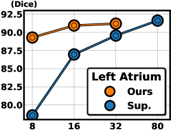
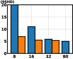
Fig. 2: Dice (left) and 95HD (right) comparison between TraCoCo (Ours) and fully supervised (Sup.) trained with 8, 16, 32 partition protocols and fully labelled data on LA dataset with VNet.

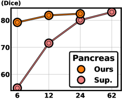
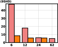
Fig. 3: Dice (left) and 95HD (right) comparison between TraCoCo (Ours) and fully supervised (Sup.) trained with 6, 12, 24 partition protocols and fully labelled data on Pancreas dataset with VNet.

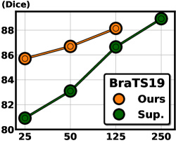
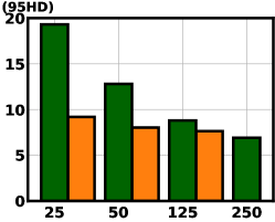
Fig. 4: Dice (left) and 95HD (right) comparison between TraCoCo (Ours) and fully supervised (Sup.) trained with 25, 50, 125 partition protocols and fully labelled data on BraTS19 dataset with VNet.

We compare our results with the fully supervised learning (trained with the same labelled set indicated by the partition protocol) using VNet on LA in Fig. 2, VNet on Pancreas in Fig. 3, and 3D-UNet on BRaTS19 in Fig. 4. Those three figures demonstrate that our approach successfully leverages unlabelled data and brings a dramatic performance boost. Particularly in the few-labelled data setup, our approach shows a $8.26\%$ Dice improvement for $8$ labelled samples on LA, $24.28\%$ for $6$ labelled samples on Pancreas, and $4.1\%$ for $25$ labelled samples on BRaTS19. Our approach yields consistent improvements for more labelled data, such as $3.59\%$ and $2.41\%$ for $16$ and $32$ volumes, respectively, on LA, and $2.85\%$ and $1.49\%$ for $50$ and $125$ volumes, respectively, on BRaTS19. Such improvements are achieved without bringing any additional computational costs for our approach during the inference phase, unlike the methods that utilise extra networks [45, 25] or multi-scales [29, 44] to explore the consistency learning.

4.6 Ablation Study of Components

Table 4: Component ablation studies on (16-label protocol) LA and (12-label protocol) Pancreas datasets: Co-Training replaces our proposed $\ell_{crc}(.)$ in the semi-supervised loss (6) by a common MSE loss, CRC denotes our proposed semi-supervised loss (6) with $\ell_{crc}(.)$ in (7), TraCo represents the translation consistency loss $\ell_{tra}(.)$ in (3), and the 3D-CutMix is in (8).

Co-Training	CRC	TraCo	3D-CutMix	LA [48]				Pancreas [9]
				Dice $\uparrow$	Jaccard $\uparrow$	ASD $\downarrow$	95HD $\downarrow$	Dice $\uparrow$	Jaccard $\uparrow$	ASD $\downarrow$	95HD $\downarrow$
$\surd$				88.82	80.29	1.95	7.42	77.69	64.39	1.82	9.91
$\surd$	$\surd$			89.84	81.66	1.91	6.46	80.64	68.11	2.03	9.66
$\surd$	$\surd$	$\surd$		90.73	82.97	1.82	6.15	81.44	69.13	1.68	5.42
$\surd$	$\surd$	$\surd$	$\surd$	90.94	83.47	1.79	5.49	81.80	69.56	1.49	5.70

We first present the ablation studies of the different components of our approach on LA [48] and Pancreas [9] datasets in Tab. 4. We use as baseline the co-training [35] with MSE loss replacing our proposed $\ell_{crc}(.)$ in the semi-supervised loss (6) by a common MSE loss (first row in Tab. 4). Replacing the MSE loss in the semi-supervised loss (6) by our CRC loss $\ell_{crc}(.)$ in (7) brings $1.52\%$ and $2.95\%$ Dice improvements in LA and Pancreas, respectively. Such improvements demonstrate that the model becomes sensitive to the foreground objects with the strict penalisation of our CRC loss. The introduction of the translation consistency loss $\ell_{tra}(.)$ from (3) is shown to improve generalisation with further Dice improvements in LA and Pancreas of $0.89\%$ and $1.80\%$, respectively. The 3D-CutMix redefines the semi-supervised loss (8) and yields Dice improvements in LA and Pancreas of $0.21\%$ and $0.36\%$, respectively.

4.7 Ablation Study of Loss functions

Table 5: Loss ablation studies on (16-label protocol) LA and (12-label protocol) Pancreas datasets. We study our TraCoCo with all components, but using different types of semi-supervised losses in (6), including MSE, KL, CE and our proposed CRC from (7).

$\ell_{sup}$	$\ell_{sem}$				LA [48]				Pancreas [9]
	MSE	KL	CE	CRC	Dice $\uparrow$	Jaccard $\uparrow$	ASD $\downarrow$	95HD $\downarrow$	Dice $\uparrow$	Jaccard $\uparrow$	ASD $\downarrow$	95HD $\downarrow$
$\surd$	$\surd$				89.77	81.49	1.73	6.80	80.29	67.71	1.21	6.10
$\surd$		$\surd$			90.01	81.88	1.86	7.83	80.94	68.33	1.78	6.97
$\surd$			$\surd$		90.50	82.71	1.84	6.74	81.26	69.07	1.64	5.81
$\mathbf{\surd}$				$\mathbf{\surd}$	90.94	83.47	1.79	5.49	81.80	69.56	1.49	5.70

Table 6: Post-processing with Connected-component Thresholding (CCT) on LA, BraTS19 and Pancreas datasets. CCT mitigates the issue of foreground noisy FP segmentation by trading off a minor computation cost increase during inference. $\dagger$ denotes the results are from best checkpoint evaluation protocol and the best results are in bold.

dataset	Post-Process	10% labelled data				20% labelled data				Time
		Dice $\uparrow$	Jaccard $\uparrow$	ASD $\downarrow$	95HD $\downarrow$	Dice $\uparrow$	Jaccard $\uparrow$	ASD $\downarrow$	95HD $\downarrow$
LA	W/O CCT	89.29	80.82	2.28	6.92	90.94	83.47	1.79	5.49	1.386 (sec/case)
	With CCT	89.31	80.83	2.09	6.83	90.96	83.49	1.70	5.45	1.412 (sec/case)
	W/O CCT ${\dagger}$	89.86	81.70	2.01	6.81	91.51	84.40	1.79	5.63	1.386 (sec/case)
	With CCT ${\dagger}$	89.94	81.85	1.72	6.67	91.62	84.59	1.45	5.36	1.412 (sec/case)
Pancreas	W/O CCT	79.22	66.04	2.57	8.46	81.80	69.56	1.49	5.70	9.892 (sec/case)
	With CCT	79.46	66.35	1.89	7.26	81.99	69.81	1.12	5.27	9.975 (sec/case)
BraTS19	W/O CCT	85.71	76.39	2.27	9.20	86.69	77.69	1.93	8.04	3.489 (sec/case)
	With CCT	85.79	76.45	2.11	8.43	86.73	77.75	1.75	7.69	3.587 (sec/case)

In Tab. 5, we study different types of loss functions to be used by the semi-supervised loss $\ell_{sem}(.)$ in (6) on both LA and Pancreas datasets. Comparing with our CRC loss (7), the KL divergence shows a $1.14\%$ worse Dice, while the CE loss, which disregards pseudo-label confidence, decreases Dice by around $0.78\%$. If we replace the CRC loss by the commonly used MSE loss [51, 21, 11, 40, 22, 45, 44], we see a drop of almost $1.39\%$ Dice on LA dataset and $1.51\%$ on Pancreas dataset. We also observe that ASD for our CRC loss is slightly larger than that for the MSE loss, which can be explained by the fact that CRC is more sensitive than MSE to the presence of foreground objects without relying too much on background information, making it vulnerable to false positive detection due to noisy predictions from hard inliers. This trade-off has a negligible impact on the voxel measurement 95HD, which calculates the 95th percentile of distances between boundary points, thus discounting the negative impact caused by these rare noisy predictions. Conversely, MSE loss tends to rely too much on background features, resulting in unsatisfactory results for all other measurements, such as Dice, mIoU, and 95HD. In next section, we present a simple post-processing technique that can mitigate the foreground noisy predictions from CRC loss. We conclude this section with a demonstration of the superior capability of our CRC loss to segment foreground objects, compared with MSE loss. We show a histogram of confidence distribution for foreground and background voxels in Fig. 5 using the Pancreas-CT dataset. Note that the CRC loss enables a tighter clustering of foreground and background voxels around confidence values of 1 and 0, respectively. This will enable a more effective classification of foreground and background voxels

4.8 Connected Component Post-processing

Connected component post-processing is a common approach to improve accuracy in medical image segmentation [13, 53, 16], where isolated false positive (FP) outlier predictions are eliminated with non-max suppression (NMS) [13, 21] or connected-component thresholding (CCT) [16]. In our work, we filter out the noisy regions that are smaller than $\mathbf{\frac{1}{1500}}$ of the input volume to remove isolated FP regions. As shown in Tab. 6, CCT yields the best results for all the measurements with the filtering out of small isolated regions. Additionally, our results with CCT produce the SOTA results in the field in all three datasets for all measures.

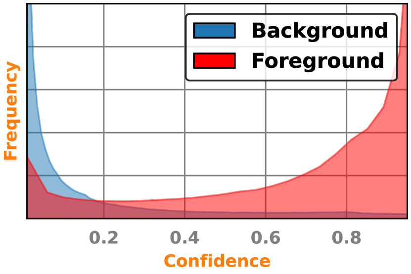
(a) MSE Loss

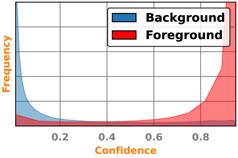
(b) CRC Loss

Fig. 5: Histogram of background and foreground confidence values in the Pancreas-CT dataset based on MSE (graph on the left) and our CRC (graph on the right) losses.

Also in Tab. 6, we evaluate the run-time of our approach with and without CCT post-processing based on cc3d python package, following SASSNet [21]. For images in the LA dataset, our method without CCT, runs in $\mathbf{1.386}$ (sec/volume) on average and in $\mathbf{1.412}$ (sec/volume) with CCT. Furthermore, our method with CCT only needs an extra $\mathbf{0.098}$ sec and $\mathbf{0.083}$ sec in BraTS19 and Pancreas, respectively.

5 Visualisation Results

Fig. 8 shows visualisation results by SASSNet [21], UA-MT [51], fully supervised, and our TraCoCo on Pancreas (with 12-label protocol – first row), LA (with 16-label protocol – second row), and BRaTS19 (with 25-label protocol – third row). It can be noted that in all cases, the visual results from our method appears to be closer to the ground truth than the results from competing approaches, particularly when considering the regions marked with a red arrow or ellipse.

Ground truth

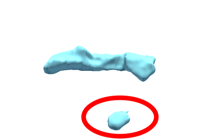
SASSNet [21]

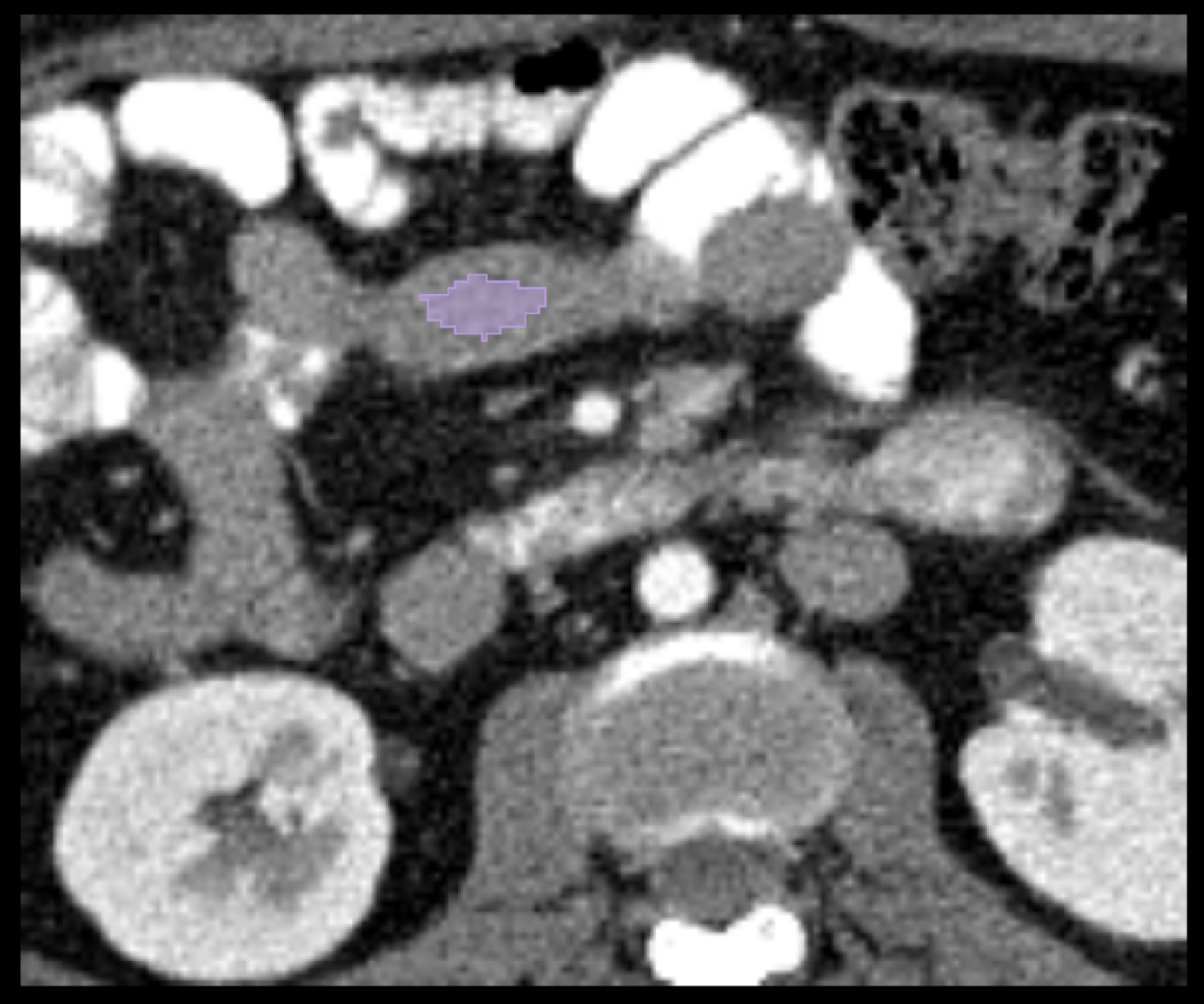
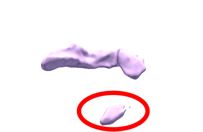
UA-MT [51]

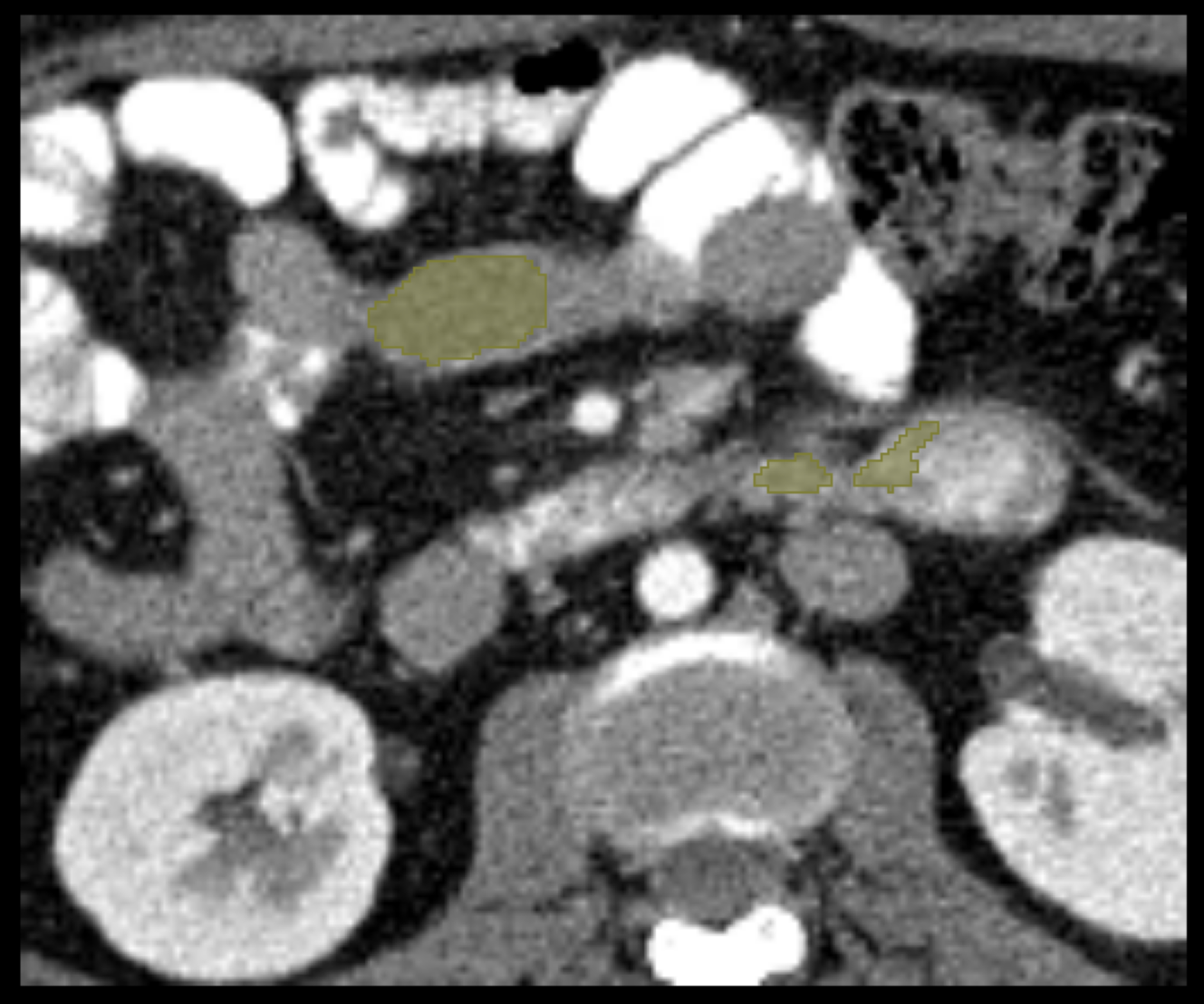
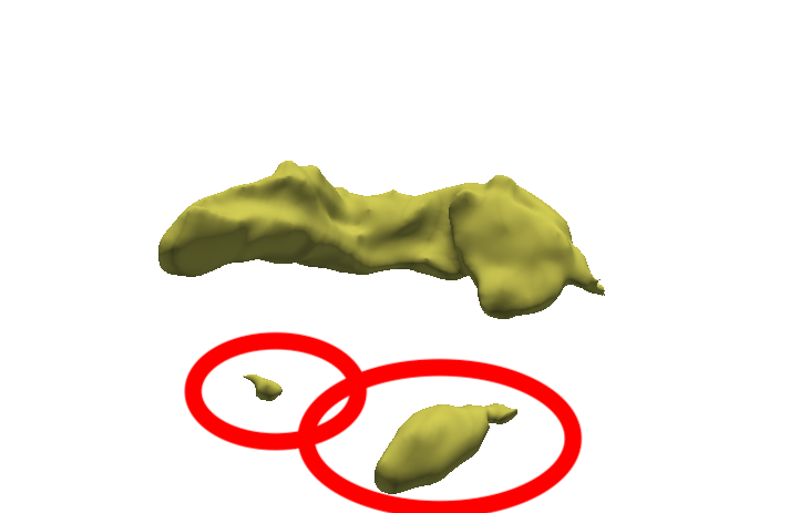
Sup. Only

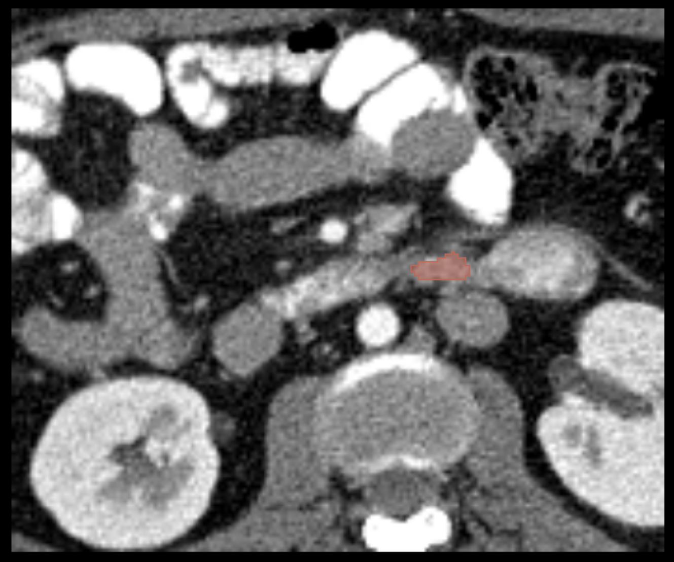
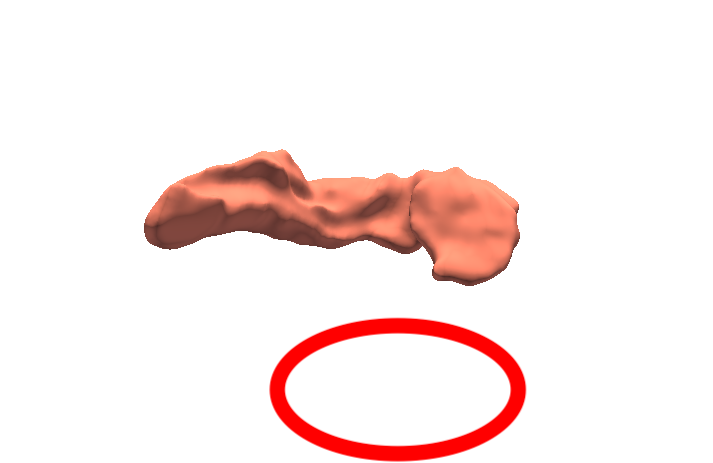
Ours

(a) Results on the $12$-labelled data partition protocol of the Pancreas-CT dataset

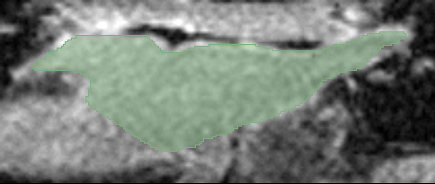
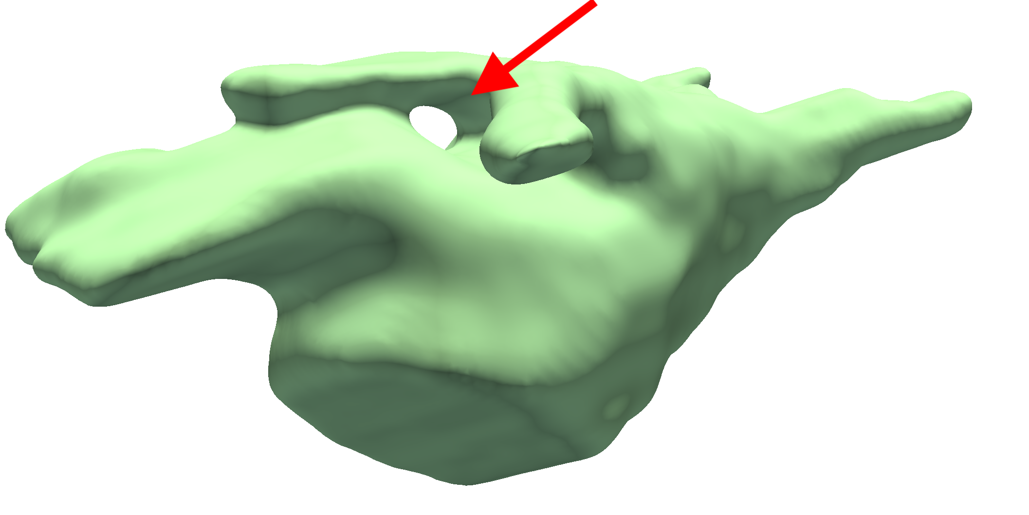
Ground truth

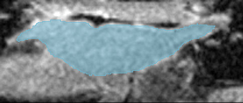
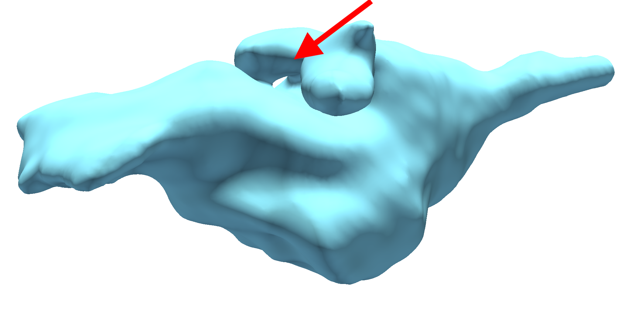
SASSNet [21]

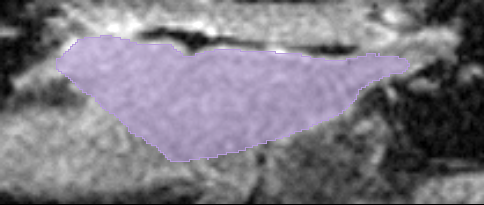
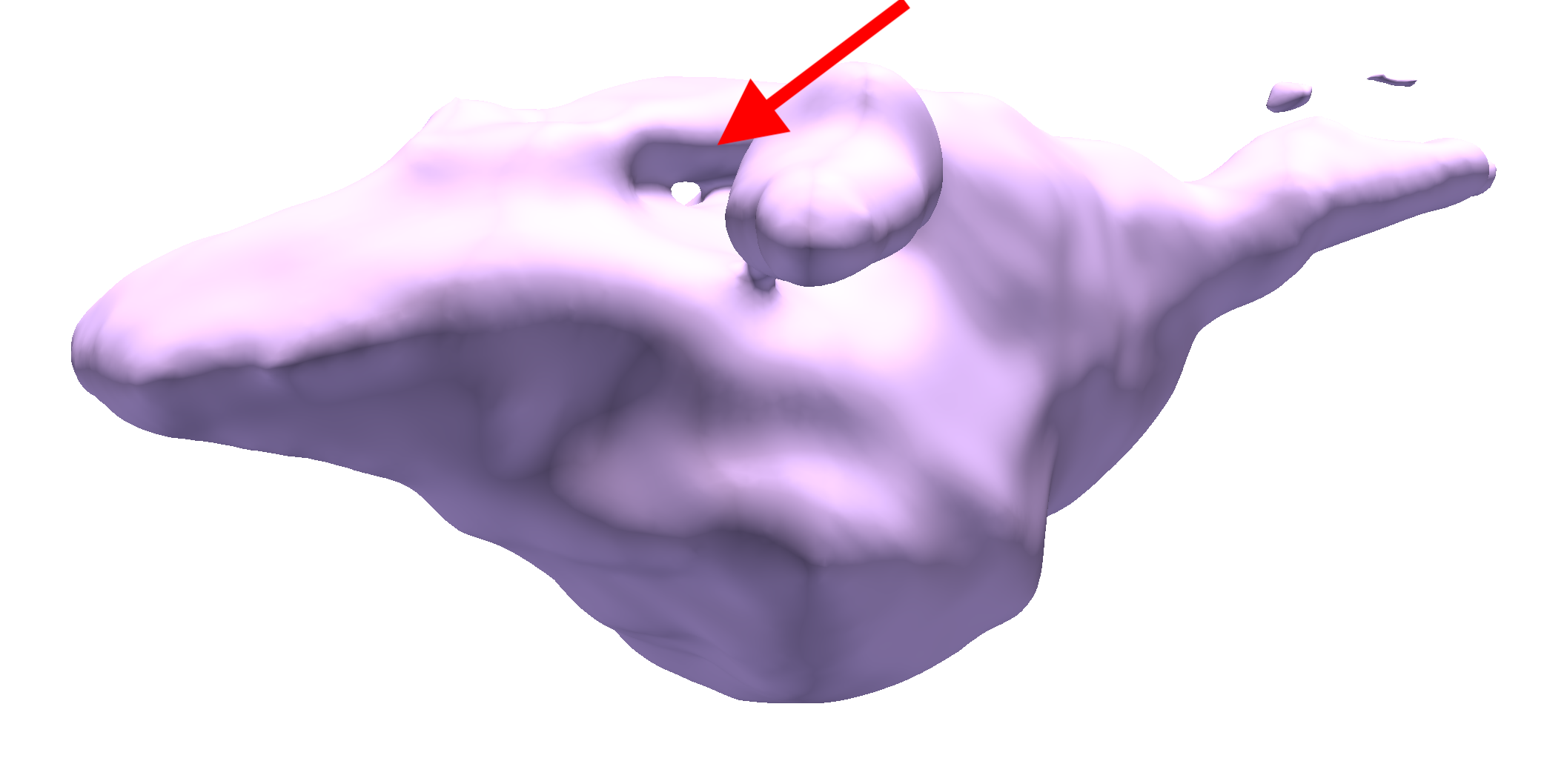
UA-MT [51]

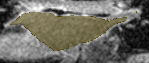
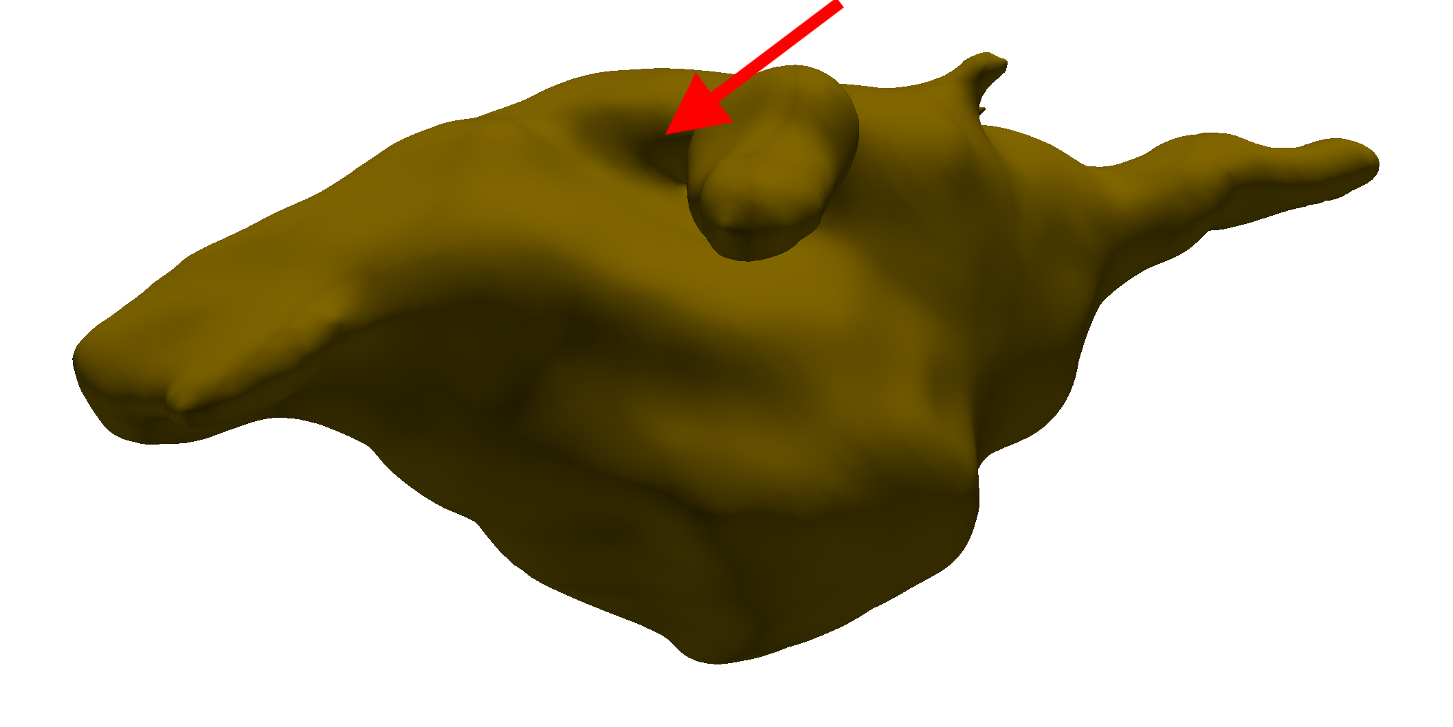
Sup. Only

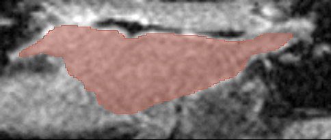
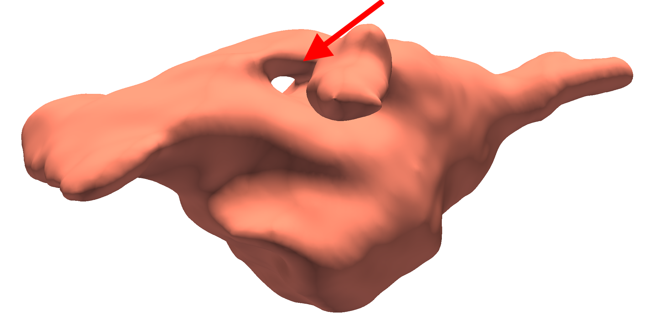
Ours

(b) Results on the $16$-labelled data partition protocol of the LA dataset

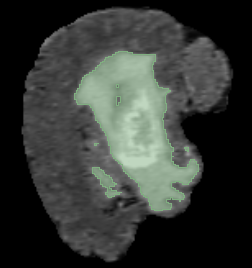
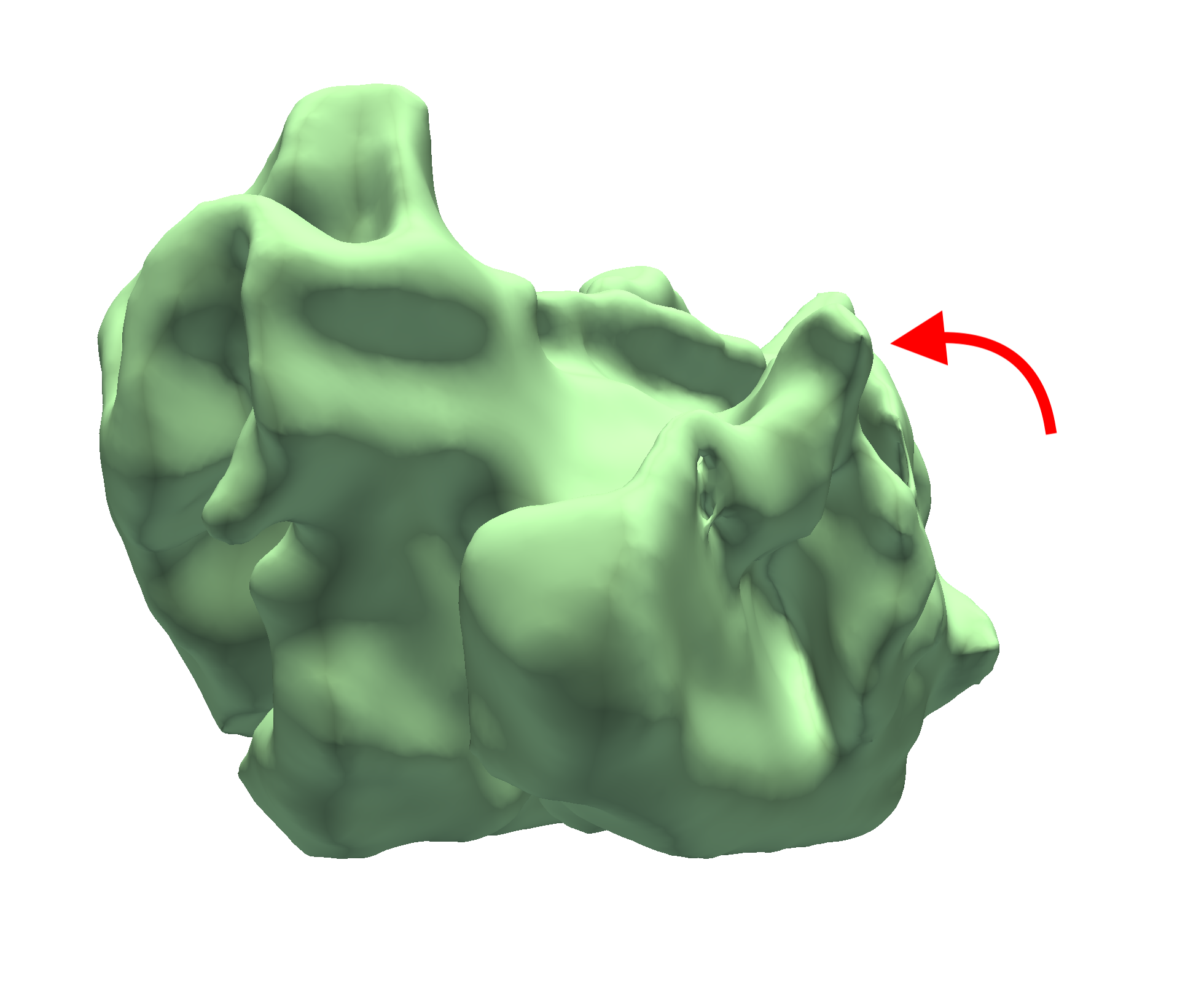
Ground truth

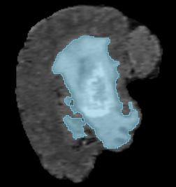
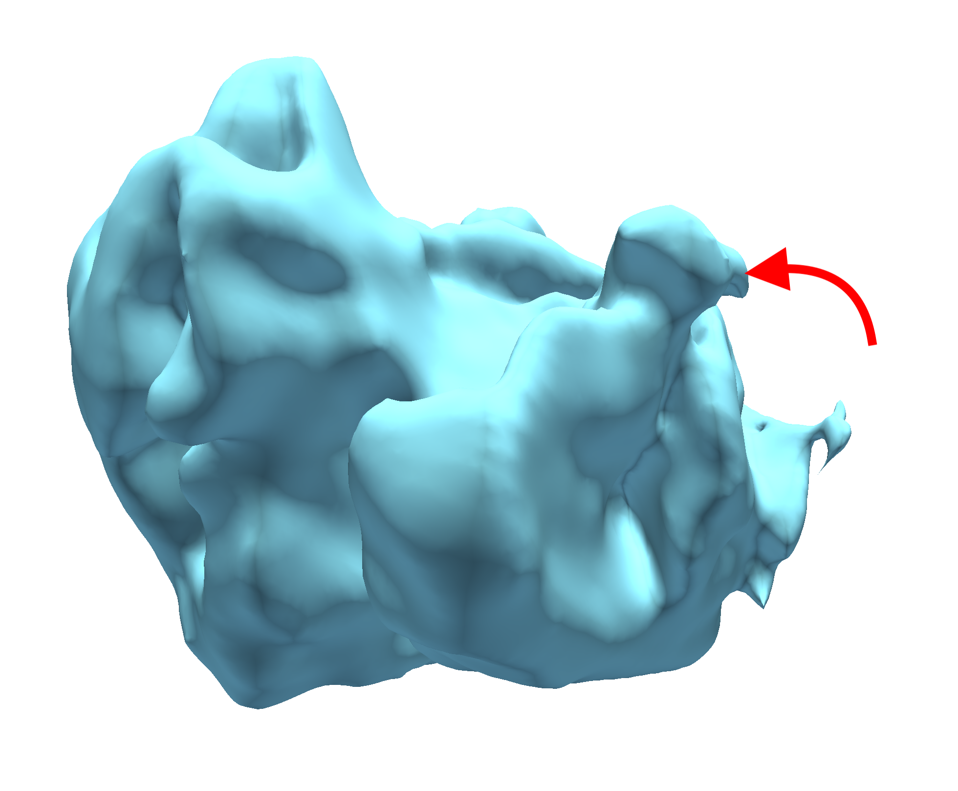
SASSNet [21]

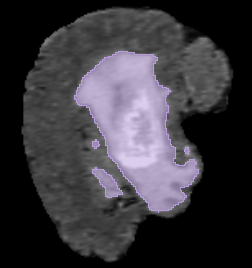
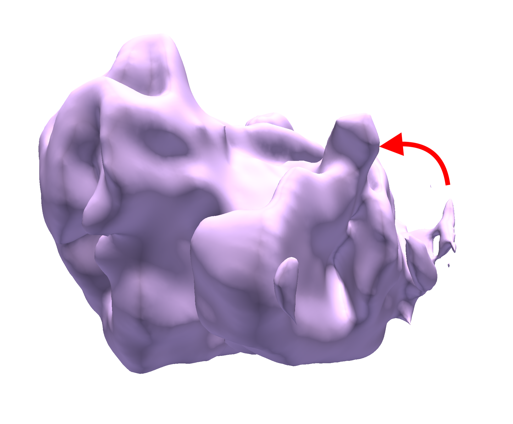
UA-MT [51]

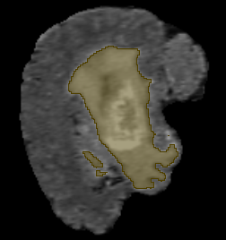
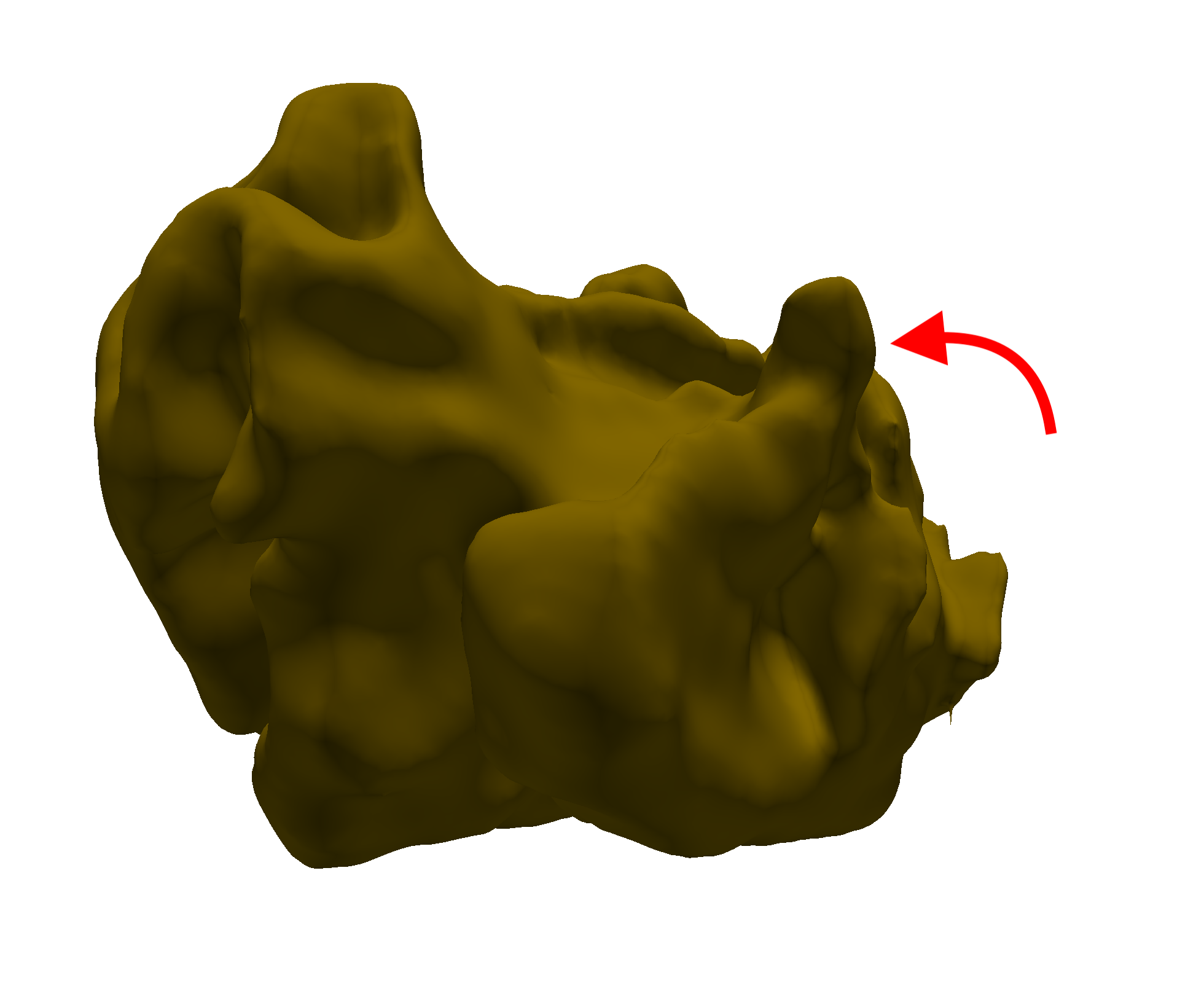
Sup. Only

Ours

(c) Results on the $25$-labelled data partition protocol of the BraTS19 dataset

Fig. 8: Qualitative segmentation results. Examples of segmentation results produced by SASSNet [21], UA-MT [51], fully supervised (Sup. Only), and our TraCoCo on Pancreas (with 12-label protocol – first row), LA (with 16-label protocol – second row), and BRaTS19 (with 25-label protocol – third row). Please notice the red arrow and ellipse markers that indicate the regions to focus on in the comparison between methods.

6 Conclusions

In this paper, we presented TraCoCo, which is a new type of consistency learning SSL method that perturbs the input data views by varying the input data spatial context to reduce the dependencies between segmented objects and background patterns. Moreover, our proposed CRC loss trains one model based on the other model’s confident predictions, yielding a better convergence than other SSL losses. The comparison with the SOTA shows that our approach produces the most accurate segmentation results on LA, Pancreas and BRaTS19 datasets. In the future, in order to deal with the the running time challenge for large volumes, more attention will be drawn to reduce the small noisy predictions while keep the sensitiveness for the foreground objects.

References

- Berthelot et al. [2019] Berthelot, D., Carlini, N., Goodfellow, I., Papernot, N., Oliver, A., Raffel, C., 2019. Mixmatch: A holistic approach to semi-supervised learning. arXiv preprint arXiv:1905.02249 .
- Blum and Mitchell [1998] Blum, A., Mitchell, T., 1998. Combining labeled and unlabeled data with co-training, in: Proceedings of the eleventh annual conference on Computational learning theory, pp. 92–100.
- Chen et al. [2020] Chen, J., Shah, V., Kyrillidis, A., 2020. Negative sampling in semi-supervised learning, in: International Conference on Machine Learning, PMLR. pp. 1704–1714.
- Chen et al. [2017] Chen, L.C., Papandreou, G., Schroff, F., Adam, H., 2017. Rethinking atrous convolution for semantic image segmentation. arXiv preprint arXiv:1706.05587 .
- Chen et al. [2018] Chen, L.C., Zhu, Y., Papandreou, G., Schroff, F., Adam, H., 2018. Encoder-decoder with atrous separable convolution for semantic image segmentation, in: Proceedings of the European conference on computer vision (ECCV), pp. 801–818.
- Chen et al. [2019] Chen, S., Bortsova, G., Juárez, A.G.U., van Tulder, G., de Bruijne, M., 2019. Multi-task attention-based semi-supervised learning for medical image segmentation, in: International Conference on Medical Image Computing and Computer-Assisted Intervention, Springer. pp. 457–465.
- Chen et al. [2021] Chen, X., Yuan, Y., Zeng, G., Wang, J., 2021. Semi-supervised semantic segmentation with cross pseudo supervision, in: IEEE Conference on Computer Vision and Pattern Recognition (CVPR).
- Çiçek et al. [2016] Çiçek, Ö., Abdulkadir, A., Lienkamp, S.S., Brox, T., Ronneberger, O., 2016. 3d u-net: learning dense volumetric segmentation from sparse annotation, in: International conference on medical image computing and computer-assisted intervention, Springer. pp. 424–432.
- Clark et al. [2013] Clark, K., Vendt, B., Smith, K., Freymann, J., Kirby, J., Koppel, P., Moore, S., Phillips, S., Maffitt, D., Pringle, M., et al., 2013. The cancer imaging archive (tcia): maintaining and operating a public information repository. Journal of digital imaging 26, 1045–1057.
- French et al. [2019] French, G., Laine, S., Aila, T., Mackiewicz, M., Finlayson, G., 2019. Semi-supervised semantic segmentation needs strong, varied perturbations. arXiv preprint arXiv:1906.01916 .
- Hang et al. [2020] Hang, W., Feng, W., Liang, S., Yu, L., Wang, Q., Choi, K.S., Qin, J., 2020. Local and global structure-aware entropy regularized mean teacher model for 3d left atrium segmentation, in: International Conference on Medical Image Computing and Computer-Assisted Intervention, Springer. pp. 562–571.
- Huang et al. [2019] Huang, Z., Wang, X., Huang, L., Huang, C., Wei, Y., Liu, W., 2019. Ccnet: Criss-cross attention for semantic segmentation, in: Proceedings of the IEEE/CVF international conference on computer vision, pp. 603–612.
- Isensee et al. [2021] Isensee, F., Jaeger, P.F., Kohl, S.A., Petersen, J., Maier-Hein, K.H., 2021. nnu-net: a self-configuring method for deep learning-based biomedical image segmentation. Nature methods 18, 203–211.
- Ishida et al. [2017] Ishida, T., Niu, G., Hu, W., Sugiyama, M., 2017. Learning from complementary labels. Advances in neural information processing systems 30.
- Ke et al. [2020] Ke, Z., Qiu, D., Li, K., Yan, Q., Lau, R.W., 2020. Guided collaborative training for pixel-wise semi-supervised learning, in: Computer Vision–ECCV 2020: 16th European Conference, Glasgow, UK, August 23–28, 2020, Proceedings, Part XIII 16, Springer. pp. 429–445.
- Khanna et al. [2020] Khanna, A., Londhe, N.D., Gupta, S., Semwal, A., 2020. A deep residual u-net convolutional neural network for automated lung segmentation in computed tomography images. Biocybernetics and Biomedical Engineering 40, 1314–1327.
- Kim et al. [2019] Kim, Y., Yim, J., Yun, J., Kim, J., 2019. Nlnl: Negative learning for noisy labels, in: Proceedings of the IEEE/CVF international conference on computer vision, pp. 101–110.
- Kim et al. [2021] Kim, Y., Yun, J., Shon, H., Kim, J., 2021. Joint negative and positive learning for noisy labels, in: Proceedings of the IEEE/CVF Conference on Computer Vision and Pattern Recognition, pp. 9442–9451.
- Lai et al. [2021] Lai, X., Tian, Z., Jiang, L., Liu, S., Zhao, H., Wang, L., Jia, J., 2021. Semi-supervised semantic segmentation with directional context-aware consistency, in: Proceedings of the IEEE/CVF Conference on Computer Vision and Pattern Recognition, pp. 1205–1214.
- Laine and Aila [2016] Laine, S., Aila, T., 2016. Temporal ensembling for semi-supervised learning. arXiv preprint arXiv:1610.02242 .
- Li et al. [2020] Li, S., Zhang, C., He, X., 2020. Shape-aware semi-supervised 3d semantic segmentation for medical images, in: International Conference on Medical Image Computing and Computer-Assisted Intervention, Springer. pp. 552–561.
- Li et al. [2021] Li, S., Zhao, Z., Xu, K., Zeng, Z., Guan, C., 2021. Hierarchical consistency regularized mean teacher for semi-supervised 3d left atrium segmentation. arXiv preprint arXiv:2105.10369 .
- Li et al. [2019] Li, X., Zhong, Z., Wu, J., Yang, Y., Lin, Z., Liu, H., 2019. Expectation-maximization attention networks for semantic segmentation, in: Proceedings of the IEEE/CVF International Conference on Computer Vision, pp. 9167–9176.
- Liu et al. [2021] Liu, Y., Tian, Y., Chen, Y., Liu, F., Belagiannis, V., Carneiro, G., 2021. Perturbed and strict mean teachers for semi-supervised semantic segmentation. arXiv preprint arXiv:2111.12903 .
- Liu et al. [2022] Liu, Y., Wang, W., Luo, G., Wang, K., Li, S., 2022. A contrastive consistency semi-supervised left atrium segmentation model. Computerized Medical Imaging and Graphics 99, 102092.
- Long et al. [2015] Long, J., Shelhamer, E., Darrell, T., 2015. Fully convolutional networks for semantic segmentation, in: Proceedings of the IEEE conference on computer vision and pattern recognition, pp. 3431–3440.
- Luo et al. [2020] Luo, L., Yu, L., Chen, H., Liu, Q., Wang, X., Xu, J., Heng, P.A., 2020. Deep mining external imperfect data for chest x-ray disease screening. IEEE transactions on medical imaging 39, 3583–3594.
- Luo et al. [2021a] Luo, X., Chen, J., Song, T., Wang, G., 2021a. Semi-supervised medical image segmentation through dual-task consistency, pp. 8801–8809.
- Luo et al. [2021b] Luo, X., Liao, W., Chen, J., Song, T., Chen, Y., Zhang, S., Chen, N., Wang, G., Zhang, S., 2021b. Efficient semi-supervised gross target volume of nasopharyngeal carcinoma segmentation via uncertainty rectified pyramid consistency, in: Medical Image Computing and Computer Assisted Intervention – MICCAI 2021, pp. 318–329.
- Mehrtash et al. [2020] Mehrtash, A., Wells, W.M., Tempany, C.M., Abolmaesumi, P., Kapur, T., 2020. Confidence calibration and predictive uncertainty estimation for deep medical image segmentation. IEEE transactions on medical imaging 39, 3868–3878.
- Menze et al. [2014] Menze, B.H., Jakab, A., Bauer, S., Kalpathy-Cramer, J., Farahani, K., Kirby, J., Burren, Y., Porz, N., Slotboom, J., Wiest, R., et al., 2014. The multimodal brain tumor image segmentation benchmark (brats). IEEE transactions on medical imaging 34, 1993–2024.
- Milletari et al. [2016] Milletari, F., Navab, N., Ahmadi, S.A., 2016. V-net: Fully convolutional neural networks for volumetric medical image segmentation, in: 2016 fourth international conference on 3D vision (3DV), Ieee. pp. 565–571.
- Minaee et al. [2021] Minaee, S., Boykov, Y.Y., Porikli, F., Plaza, A.J., Kehtarnavaz, N., Terzopoulos, D., 2021. Image segmentation using deep learning: A survey. IEEE transactions on pattern analysis and machine intelligence .
- Ouali et al. [2020] Ouali, Y., Hudelot, C., Tami, M., 2020. Semi-supervised semantic segmentation with cross-consistency training, in: Proceedings of the IEEE/CVF Conference on Computer Vision and Pattern Recognition, pp. 12674–12684.
- Qiao et al. [2018] Qiao, S., Shen, W., Zhang, Z., Wang, B., Yuille, A., 2018. Deep co-training for semi-supervised image recognition, in: Proceedings of the european conference on computer vision (eccv), pp. 135–152.
- Rizve et al. [2021] Rizve, M.N., Duarte, K., Rawat, Y.S., Shah, M., 2021. In defense of pseudo-labeling: An uncertainty-aware pseudo-label selection framework for semi-supervised learning. arXiv preprint arXiv:2101.06329 .
- Ronneberger et al. [2015] Ronneberger, O., Fischer, P., Brox, T., 2015. U-net: Convolutional networks for biomedical image segmentation, in: Medical Image Computing and Computer-Assisted Intervention–MICCAI 2015: 18th International Conference, Munich, Germany, October 5-9, 2015, Proceedings, Part III 18, Springer. pp. 234–241.
- Tarvainen and Valpola [2017] Tarvainen, A., Valpola, H., 2017. Mean teachers are better role models: Weight-averaged consistency targets improve semi-supervised deep learning results. arXiv preprint arXiv:1703.01780 .
- Verma et al. [2019] Verma, V., Kawaguchi, K., Lamb, A., Kannala, J., Bengio, Y., Lopez-Paz, D., 2019. Interpolation consistency training for semi-supervised learning. arXiv preprint arXiv:1903.03825 .
- Wang et al. [2021] Wang, K., Zhan, B., Zu, C., Wu, X., Zhou, J., Zhou, L., Wang, Y., 2021. Tripled-uncertainty guided mean teacher model for semi-supervised medical image segmentation, in: International Conference on Medical Image Computing and Computer-Assisted Intervention, Springer. pp. 450–460.
- Wang et al. [2023] Wang, P., Peng, J., Pedersoli, M., Zhou, Y., Zhang, C., Desrosiers, C., 2023. Cat: Constrained adversarial training for anatomically-plausible semi-supervised segmentation. IEEE Transactions on Medical Imaging .
- Wang et al. [2022] Wang, T., Lu, J., Lai, Z., Wen, J., Kong, H., 2022. Uncertainty-guided pixel contrastive learning for semi-supervised medical image segmentation, in: Proceedings of the Thirty-First International Joint Conference on Artificial Intelligence, IJCAI, pp. 1444–1450.
- Wang et al. [2020] Wang, Y., Zhang, Y., Tian, J., Zhong, C., Shi, Z., Zhang, Y., He, Z., 2020. Double-uncertainty weighted method for semi-supervised learning, in: International Conference on Medical Image Computing and Computer-Assisted Intervention, Springer. pp. 542–551.
- Wu et al. [2022] Wu, Y., Ge, Z., Zhang, D., Xu, M., Zhang, L., Xia, Y., Cai, J., 2022. Mutual consistency learning for semi-supervised medical image segmentation. Medical Image Analysis 81, 102530.
- Wu et al. [2021] Wu, Y., Xu, M., Ge, Z., Cai, J., Zhang, L., 2021. Semi-supervised left atrium segmentation with mutual consistency training. arXiv preprint arXiv:2103.02911 .
- Xia et al. [2020] Xia, Y., Yang, D., Yu, Z., Liu, F., Cai, J., Yu, L., Zhu, Z., Xu, D., Yuille, A., Roth, H., 2020. Uncertainty-aware multi-view co-training for semi-supervised medical image segmentation and domain adaptation. Medical image analysis 65, 101766.
- Xiang et al. [2022] Xiang, J., Qiu, P., Yang, Y., 2022. Fussnet: Fusing two sources of uncertainty for semi-supervised medical image segmentation, in: Medical Image Computing and Computer Assisted Intervention–MICCAI 2022: 25th International Conference, Singapore, September 18–22, 2022, Proceedings, Part VIII, Springer. pp. 481–491.
- Xiong et al. [2021] Xiong, Z., Xia, Q., Hu, Z., Huang, N., Bian, C., Zheng, Y., Vesal, S., Ravikumar, N., Maier, A., Yang, X., et al., 2021. A global benchmark of algorithms for segmenting the left atrium from late gadolinium-enhanced cardiac magnetic resonance imaging. Medical image analysis 67, 101832.
- Xu et al. [2023] Xu, C., Yang, Y., Xia, Z., Wang, B., Zhang, D., Zhang, Y., Zhao, S., 2023. Dual uncertainty-guided mixing consistency for semi-supervised 3d medical image segmentation. IEEE Transactions on Big Data .
- Yang et al. [2018] Yang, M., Yu, K., Zhang, C., Li, Z., Yang, K., 2018. Denseaspp for semantic segmentation in street scenes, in: Proceedings of the IEEE conference on computer vision and pattern recognition, pp. 3684–3692.
- Yu et al. [2019] Yu, L., Wang, S., Li, X., Fu, C.W., Heng, P.A., 2019. Uncertainty-aware self-ensembling model for semi-supervised 3d left atrium segmentation, in: International Conference on Medical Image Computing and Computer-Assisted Intervention, Springer. pp. 605–613.
- Yun et al. [2019] Yun, S., Han, D., Oh, S.J., Chun, S., Choe, J., Yoo, Y., 2019. Cutmix: Regularization strategy to train strong classifiers with localizable features, in: Proceedings of the IEEE/CVF International Conference on Computer Vision, pp. 6023–6032.
- Zhao and Zeng [2019] Zhao, W., Zeng, Z., 2019. Multi scale supervised 3d u-net for kidney and tumor segmentation. arXiv preprint arXiv:1908.03204 .
- Zheng et al. [2019] Zheng, H., Lin, L., Hu, H., Zhang, Q., Chen, Q., Iwamoto, Y., Han, X., Chen, Y.W., Tong, R., Wu, J., 2019. Semi-supervised segmentation of liver using adversarial learning with deep atlas prior, in: International Conference on Medical Image Computing and Computer-Assisted Intervention, Springer. pp. 148–156.
- Zhou et al. [2018] Zhou, Z., Rahman Siddiquee, M.M., Tajbakhsh, N., Liang, J., 2018. Unet++: A nested u-net architecture for medical image segmentation, in: Deep Learning in Medical Image Analysis and Multimodal Learning for Clinical Decision Support: 4th International Workshop, DLMIA 2018, and 8th International Workshop, ML-CDS 2018, Held in Conjunction with MICCAI 2018, Granada, Spain, September 20, 2018, Proceedings 4, Springer. pp. 3–11.