Certified Mergeable Replicated Data Types
(Extended Version)

Abstract.

Replicated data types (RDTs) are data structures that permit concurrent modification of multiple, potentially geo-distributed, replicas without coordination between them. RDTs are designed in such a way that conflicting operations are eventually deterministically reconciled ensuring convergence. Constructing correct RDTs remains a difficult endeavour due to the complexity of reasoning about independently evolving states of the replicas. With the focus on the correctness of RDTs (and rightly so), existing approaches to RDTs are less efficient compared to their sequential counterparts in terms of time- and space-complexity of local operations. This is unfortunate since RDTs are often used in an local-first setting where the local operations far outweigh remote communication.

In this paper, we present Peepul, a pragmatic approach to building and verifying efficient RDTs. To make reasoning about correctness easier, we cast RDTs in the mould of distributed version control system, and equip it with a three-way merge function for reconciling conflicting versions. Further, we go beyond just verifying convergence, and provide a methodology to verify arbitrarily complex specifications. We develop a replication-aware simulation relation to relate RDT specifications to their efficient purely functional implementations. We have developed Peepul as an F* library that discharges proof obligations to an SMT solver. The verified efficient RDTs are extracted as OCaml code and used in Irmin, a Git-like distributed database.

1. Introduction

Modern cloud-based software services often replicate data across multiple geographically distributed locations in order to tolerate against partial failures of servers and to minimise latency by bringing data closer to the user. While services like Google Docs allow several users to concurrently edit the document, the conflicts are resolved with the help of a centralised server. On the other hand, services like Github and Gitlab, built on the decentralised version control system Git, avoid the need for a centralised server, and permit the different replicas (forks) to synchronize with each other in a peer-to-peer fashion. By avoiding centralised server, local-first software (Kleppmann et al., 2019) such as Git bring in additional benefits of security, privacy and user ownership of data.

While Git is designed for line-based editing of text files and requires manual intervention in the presence of merge conflicts, RDTs generalise this concept to arbitrary general purpose data structures such as lists and hash maps, and ensure convergence without manual intervention. Convergent Replicated Data Types (CRDTs) (Shapiro et al., 2011), which arose from distributed systems research, are complete reimplementations of sequential counterparts aimed at providing convergence without user intervention, and have been deployed in distributed data bases such as AntidoteDB (Shapiro et al., 2018) and Riak (Riak, 2021).

In order to resolve conflicting updates, CRDTs generally need to carry their causal contexts as metadata (Yu and Rostad, 2020). Managing this causal context is often expensive and complicated. For example, consider the observed-removed set CRDT (OR-set) (Shapiro et al., 2011), where, in the case of concurrent addition and removal, the addition wins. A typical OR-set implementation uses two grow-only sets, one for elements added to the set $\mathcal{A}$ and another for elements that are removed $\mathcal{R}$. An element $e$ is removed from the OR-set by adding it to the set $\mathcal{R}$, and thus creating a tombstone for $e$. The set membership is given by the difference between the two: $\mathcal{A}-\mathcal{R}$, and two concurrent versions can be merged by unioning the individual $\mathcal{A}$ and $\mathcal{R}$ sets. Observe that the tombstones for removed elements cannot be garbage collected as that would require all the replicas to remove the element at the same time, which requires global coordination. This leads to an inefficient implementation. Several techniques have been proposed to minimise this metadata overhead (Yu and Rostad, 2020; Almeida et al., 2018), but the fundamental problem still remains.

1.1. Mergeable Replicated Data Types

As an alternative to CRDTs, mergeable replicated data types (MRDTs) (Kaki et al., 2019) have been proposed, which extend the idea of distributed version control for arbitrary data types. The causal context necessary for resolving the conflicts is maintained by the MRDT middleware. MRDTs allow ordinary purely functional data structures (Okasaki, 1999) to be promoted to RDTs by equipping them with a three-way merge function that describes the conflict resolution policy. When conflicting updates need to be reconciled, the causal history is used to determine the lowest common ancestor (lca) for use in the three-way merge function along with the conflicting states. The MRDT middleware garbage collects the causal histories when appropriate (Dubey, 2021), and is no longer a concern for the RDT library developer. This branch-consistent view of replication not only makes it easier to develop individual data types, but also leads to a natural transactional semantics (Crooks et al., 2016; Dubey et al., 2020).

An efficient OR-set MRDT that avoids tombstones can be implemented as follows. We represent the OR-set as a list of pairs of the element and a unique id, which is generated per operation. The list may have duplicate elements with different ids. Adding an element appends the element and the id pair to the head of the list ($O(1)$ operation). Removing an element removes all the occurrences of the element from the list ($O(n)$ operation). Given two concurrent versions of the OR-set $a$ and $b$, and their lowest common ancestor $l$, the merge is implemented as $(a-l)~{}@~{}(b-l)~{}@~{}(l\cap a\cap b)$, where $@$ stands for list append. Intuitively, we append the lists formed by newly added elements in $a$ and $b$ with the list of elements that are present on all the three versions. The unique id associated with the element ensures that in the presence of concurrent addition and removal of the same element, the newly added element with the fresh id, which has not been seen by the concurrent remove, will remain in the merged result. The merge operation can be implemented in $O(n~{}log~{}n)$ time by sorting the individual lists. In §2.1.2, we show how to make this implementation even more efficient by removing the duplicate elements with different ids from the OR-set.

1.2. Efficiency and correctness

The key question is how do we guarantee that such efficient implementations still preserve the intent of the OR-Set in a sound manner? Optimisations such as removing duplicate elements are notoriously difficult to get right since the replica states evolve independently. Moreover, individually correct RDTs may fail to preserve convergence when put together (Kleppmann, 2020). Kaki et al. (Kaki et al., 2019) opine that merge functions should not be written by hand, but automatically derived from a relational representation of the sequential data type. Their idea is to capture the key properties of the algebraic data type as relations over its constituent elements. Then, the merge function devolves to a merge of these relations (sets) expressed as MRDTs. During merge, the concrete implementations are reified to their relational representations expressed in terms of sets, merged using set semantics, and the final concrete state is reconstructed from the relational set representation.

Unfortunately, mapping complex data types to sets does not lead to efficient implementations. For example, a queue in Kaki et al. is represented by two characteristic relations – a unary relation for membership and a binary relation for ordering. For a queue with $n$ elements, the ordering relation contains $n^{2}$ elements. Reifying the queue to its characteristic relations and back to its concrete representation for every merge is inefficient and impractical. This technique does not scale as the structure of the data type gets richer (Red-Black tree, JSON, file systems, etc.). The more complex the data type, more complex the characteristic relations become, having an impact on the cost of merge. Further Kaki et al. do not consider functional correctness of MRDT implementations, but instead only focuses on the correctness of convergence.

1.3. Certified MRDTs

Precisely specifying and verifying the functional correctness of efficient RDT implementations is not straightforward due to the complexity of handling conflicts between divergent versions. This results in a huge gap between the high-level specifications and efficient implementations. In this work, we propose to bridge this gap by using Burckhardt et al.’s replication-aware simulation relation (Burckhardt et al., 2014). However, Burckhardt et al.’s simulation is only applicable to CRDTs and cannot be directly extended to MRDTs which assume a different system model.

We first propose a system model and an operational semantics for MRDTs, and precisely define the problem of convergence and functional correctness for MRDTs. We also introduce a new notion of convergence modulo observable behaviour, which allows replicas to converge to different states, as long as their observable behaviour to clients remains the same. This notion allows us to build and verify even more efficient MRDTs.

Further, we go beyond Burckhardt et al.’s work (Burckhardt et al., 2014) in the use of simulation relations by mechanizing and automating (to an extent) the complete verification process. We instantiate our technique as an F* library named Peepul and mechanically verify the implementation of a number efficient purely functional MRDT implementations including an efficient replicated two-list queue. Our replicated queue supports constant time push and pop operations, a linear time merge operation, and does not have any tombstones. To the best of our knowledge, ours is the first formal declarative specification of a distributed queue (§6), and its mechanised proof of correctness.

Being a SMT-solver-aided programming language, F* allows us to discharge many of the proof obligations automatically through the SMT solver. Even though our approach requires the simulation relation as input, we also observe that in most cases, the simulation relation directly follows from the declarative specification.

Our technique also supports composition, and we demonstrate how parametric polymorphism allows composition of not just the MRDT implementations but also their proofs of correctness. From our MRDT implementations in F*, we extract verified OCaml implementations and execute them on top of Irmin, a Git-like distributed database. Our experimental evaluation shows that our efficient MRDT implementations scale significantly better than other RDT implementations.

To summarize, we make the following contributions:

• We propose a store semantics for MRDT implementations and formally define the convergence and functional correctness problem for MRDTs, including a new notion of convergence modulo observable behaviour.

• We propose a technique to verify both convergence and functional correctness of MRDTs by adapting the notion of replication-aware simulation relation (Burckhardt et al., 2014) to the MRDT setting.

• We mechanize and automate the complete verification process using F*, and apply our technique on a number of complex MRDT implementations, including a new time and space-efficient ORSet and a queue MRDT.

• We provide experimental results which demonstrate that our efficient MRDT implementations perform much better as compared with previous implementations, and also show the tradeoff between proof automation and verification time in F*.

The rest of the paper is organized as follows. §2 presents the implementation model and the declarative specification framework for MRDTs. §3 presents the formal semantics of the git-like replicated store on which MRDT implementations run. In §4, we present a new verification strategy for MRDTs based on the notion of replication-aware simulation. §5 highlights the compositionality of our technique in verifying complex verified MRDTs reusing the proofs of simpler ones. §6 presents the formally verified efficient replicated queue. §7 presents the experimental evaluation and §8 presents the related work.

2. Implementing and Specifying MRDTs

In this section, we present the formal model for describing MRDT implementations and their specifications.

2.1. Implementation

Our model of replicated datastore is similar to a distributed version control system like Git (Git, 2021), with replication centred around versioned states in branches and explicit merges. A typical replicated datastore will have a key-value interface with the capability to store arbitrary objects as values (Riak, 2021; Irmin, 2021). Since our goal is to verify correct implementations of individual replicated objects, our formalism models a store with a single object.

A replicated datastore consists of an object which is replicated across multiple branches $b_{1},b_{2},\ldots\in branchID$. Clients interact with the store by performing operations on the object at a specified branch, modifying its local state. The different branches may concurrently update their local states and progress independently. We also allow dynamic creation of a new branch by copying the state of an existing branch. A branch at any time can get updates from any other branch by performing a merge with that branch, updating its local copy to reflect the merge. Conflicts might arise when the same object is modified in two or more branches, and these are resolved in an data type specific way.

An object has a type $\tau\in Type$, whose type signature $(Op_{\tau},Val_{\tau})$ determines the set of supported operations $Op_{\tau}$ and the set of their return values $Val_{\tau}$. A special value $\bot\in Val_{\tau}$ is used for operations that return no value.

Definition 2.1.

A mergeable replicated data type (MRDT) implementation for a data type $\tau$ is a tuple $D_{\tau}=(\Sigma,\sigma_{0},do,\allowbreak merge)$ where:

• $\Sigma$ is the set of all possible states at a branch,

• $\sigma_{0}\in\Sigma$ is the initial state,

• $do:Op_{\tau}\times\Sigma\times Timestamp\rightarrow\Sigma\times Val_{\tau}$ implements every data type operation,

• $merge:\Sigma\times\Sigma\times\Sigma\rightarrow\Sigma$ implements the three-way merge strategy.

An MRDT implementation $\mathcal{D_{\tau}}$ provides two methods: do and merge that the datastore will invoke appropriately. We assume that these methods execute atomically. A client request to perform an operation $o\in Op_{\tau}$ at a branch triggers the call $do(o,\sigma,t)$. This takes the current state $\sigma\in\Sigma$ of the object at the branch where the request is issued and a timestamp $t\in Timestamp$ provided by the datastore, and produces the updated object state and the return value of the operation.

The datastore guarantees that the timestamps are unique across all of the branches, and for any two operations $a$ and $b$, with timestamps $t_{a}$ and $t_{b}$, if $a$ happens-before $b$, then $t_{a}<t_{b}$. The data type implementation can use the timestamp provided to implement the conflict-resolution strategy, but is also free to ignore it. For simplicity of presentation, we assume that the timestamps are positive integers, $Timestamp=\mathbb{N}$. The datastore may choose to implement the timestamp using Lamport clocks (Lamport, 1978), along with the unique branch id to provide uniqueness of timestamps.

A branch $a$ may get updates from another branch $b$ by performing a merge, which modifies the state of the object in branch $a$. In this case, the datastore will invoke $merge(\sigma_{lca},\allowbreak\sigma_{a},\allowbreak\sigma_{b})$ where $\sigma_{a}$ and $\sigma_{b}$ are the current states of branch $a$ and $b$ respectively, and $\sigma_{lca}$ is the lowest common ancestor (LCA) of the two branches. The LCA of two branches is the most recent state from which the two branches diverged. We assume that execution of the store will begin with a single branch, from which new branches may be dynamically created. Hence, for any two branches, the LCA will always exist.

2.1.1. OR-set

We illustrate MRDT implementations using the example of an OR-set. Recall from §1 that the OR-set favours the addition in the case where there is a concurrent addition and removal of the same element on different branches.

1:$\Sigma=\mathcal{P}(\mathbb{N}\times\mathbb{N})$

2:$\sigma_{0}=\{\}$

3:$do(rd,\sigma,t)=(\sigma,\{a\mid(a,t)\in\sigma\})$

4:$do(add(a),\sigma,t)=(\sigma\cup\{(a,t)\},\bot)$

5:$do(remove(a),\sigma,t)=(\{e\in\sigma\mid fst(e)\neq a\},\bot)$

6:$merge(\sigma_{lca},\sigma_{a},\sigma_{b})=$

7:$(\sigma_{lca}\cap\sigma_{a}\cap\sigma_{b})\cup(\sigma_{a}-\sigma_{lca})\cup(\sigma_{b}-\sigma_{lca})$

Figure 1. OR-set data type implementation

Let us assume that the elements in the OR-set are natural numbers. Its type signature would be $(Op_{orset},Val_{orset})$ $=(\{\mathsf{add}(a),\mathsf{remove}(a)\mid a\in\mathbb{N}\}\cup\{\mathsf{rd}\},\{\mathcal{P}(\mathbb{N}),\bot\})$. Figure 1 shows an MRDT implementation of the OR-set data type. The state of the object is a set of pairs of the element and the timestamp. The operations and the merge remain the same as described in §1.1. Note that we use $fst$ and $snd$ functions to obtain the first and second elements respectively from a tuple. This implementation may have duplicate entries of the same element with different timestamps.

2.1.2. Space-efficient OR-set (OR-set-space)

One possibility to make this OR-set implementation more space-efficient is by removing the duplicate entries from the set. A duplicate element will appear in the set if the client calls $\mathsf{add}(e)$ for an element $e$ which is already in the set. Can we reimplement $\mathsf{add}$ such that we leave the set as is if the set already has $e$? Unfortunately, this breaks the intent of the OR-set. In particular, if there were a concurrent remove of $e$ on a different branch, then $e$ will be removed when the branches are merged. The key insight is that the effect of the duplicate add has to be recorded so as to not lose additions.

1:$\Sigma=\mathcal{P}(\mathbb{N}\times\mathbb{N})$

2:$\sigma_{0}=\{\}$

3:$do(rd,\sigma,t)=(\sigma,\{a\mid(a,t)\in\sigma\})$

4:$do(add(a),\sigma,t)=\text{if }(a,\_)\in\sigma\text{ then }(\sigma[a\mapsto t],\bot)$

5:$\qquad\qquad\qquad\quad\text{ else }(\sigma\cup\{(a,t)\},\bot)$

6:$do(remove(a),\sigma,t)=(\{e\in\sigma\mid fst(e)\neq a\},\bot)$

7:$merge(\sigma_{lca},\sigma_{a},\sigma_{b})=$

8:$\quad\{e\mid e\in(\sigma_{lca}\cap\sigma_{a}\cap\sigma_{b})\}~{}\cup$

9:$\quad\{e\mid e\in(\sigma_{a}-\sigma_{lca})\wedge(fst(e),\_)\notin(\sigma_{b}-\sigma_{lca})\}~{}\cup$

10:$\quad\{e\mid e\in(\sigma_{b}-\sigma_{lca})\wedge(fst(e),\_)\notin(\sigma_{a}-\sigma_{lca})\}~{}\cup$

11:$\quad\{e\mid e\in(\sigma_{a}-\sigma_{lca})~{}\wedge$

12:$\quad\quad\enskip\enskip(\forall t.~{}(fst(e),t)\in(\sigma_{b}-\sigma_{lca})\Rightarrow snd(e)>t)\}~{}\cup$

13:$\quad\{e\mid e\in(\sigma_{b}-\sigma_{lca})~{}\wedge$

14:$\quad\quad\enskip\enskip(\forall t.~{}(fst(e),t)\in(\sigma_{a}-\sigma_{lca})\Rightarrow snd(e)>t)\}$

Figure 2. Space-efficient OR-set (OR-set-space) implementation

Figure 2 provides the implementation of the space-efficient OR-set. The read and the remove operations remain the same as the earlier implementation. If the element being added is not already present in the set, then the element is added to the set along with the timestamp. Otherwise, the timestamp of the existing entry is updated to the new timestamp. Given that our timestamps are unique, the new operation’s timestamp will be distinct from the old timestamp. This prevents a concurrent remove from deleting this new addition.

Another possibility of duplicates is that the same element may concurrently be added on two different branches. The implementation of the merge function now has to take care of this possibility and not include duplicates. An element in the merged set was either in the lca and the two concurrent states (line 8), or was only added in one of the branches (lines 9 and 10), or was added in both the branches in which case we pick the entry with the larger timestamp (lines 11–14).

2.2. Specification

Given that there are several candidates for implementing an MRDT, we need a way to specify the behaviour of an MRDT so that we may ask the question of whether the given implementation satisfies the specification. We now present a declarative framework for specifying MRDTs which closely follows the framework presented by Burckhardt et al. (Burckhardt et al., 2014). We define our specifications on an abstract state, which capture the state of the distributed store. It consists of events in a execution of the distributed store, along with a visibility relation among them.

Definition 2.2.

An abstract state for a data type $\tau=(Op_{\tau},\allowbreak Val_{\tau})$ is a tuple $I=\langle E,oper,rval,time,vis\rangle$, where

• $E\subseteq Event$ is a set of events,

• $oper:E\rightarrow Op_{\tau}$ associates the data type operation with each event,

• $rval:E\rightarrow Val_{\tau}$ associates the return value with each event,

• $time:E\rightarrow Timestamp$ associates the timestamp at which an event was performed,

• $vis\subseteq E\times E$ is an irreflexive, asymmetric and transitive visibility relation.

Given $e\xrightarrow{vis}f$, $e$ is said to causally precede $f$. In our setting, it may be the case that the operation of $f$ follows the operation of $e$ on the same branch, or the operations of $f$ and $e$ were performed on different branches $b_{f}$ and $b_{e}$, but before the operation of $f$, the branch $b_{e}$ on which the operation of $e$ was performed was merged info $b_{f}$.

We specify a data type $\tau$ by a function $\mathcal{F_{\tau}}$ which determines the return value of an operation $o$ based on prior operations applied on that object. $\mathcal{F_{\tau}}$ also takes as a parameter the abstract state that is visible to the operation. Note that the abstract state contains all the information that is necessary to specify the return-value of $o$.

Definition 2.3.

A replicated data type specification for a type $\tau$ is a function $\mathcal{F_{\tau}}$ that given an operation $o\in Op_{\tau}$ and an abstract state $I$ for $\tau$, specifies a return value $\mathcal{F_{\tau}}(o,I)\in Val_{\tau}$.

2.2.1. OR-set specification

As an illustration of the specification language, let us consider the OR-set. For the OR-set, both $\mathsf{add}$ and $\mathsf{remove}$ operations always return $\bot$. We can formally specify the ‘add-wins’ conflict resolution strategy as follows:

$$\mathcal{F}_{orset}(\mathsf{rd},\langle E,oper,rval,time,vis\rangle)=\{a\mid\exists e\in E.\ oper(e)$$

$$=\mathsf{add}(a)\wedge\neg(\exists f\in E.\ oper(f)=\mathsf{remove}(a)\wedge e\xrightarrow{vis}f)\}$$

In words, the read operation returns all those elements for which there exists an $\mathsf{add}$ operation of the element which is not visible to a $\mathsf{remove}$ operation of the same element. Hence, if an $\mathsf{add}$ and $\mathsf{remove}$ operation are concurrent, then the $\mathsf{add}$ would win. Notice that the specification, while precisely encoding the required semantics, is far removed from the MRDT implementations of the OR-set that we saw earlier. Providing a framework for bridging this gap in an automated and mechanized manner is one of the principal contributions of this work.

3. Store Semantics and MRDT Correctness

In this section, we formally define the semantics of a replicated datastore $\mathbb{S}$ consisting of a single object with data type implementation $\mathcal{D}_{\tau}$. Note that the store semantics can be easily generalized to multiple objects (with possibly different data types), since the store treats each object independently. We then define formally what it means for data type implementations to satisfy their specifications. We also introduce a novel notion of convergence across all the branches called convergence modulo observable behaviour that differs from the standard notions of eventual consistency. This property allows us to have more efficient but verified merges.

The semantics of the store is a set of all its executions. In order to easily relate the specifications which are in terms of abstract states to the implementation, we maintain both the concrete state (as given by the data type implementation) and the abstract state at every branch in our store semantics. Formally, the semantics of the store are parametrised by a data type $\tau$ and its implementation $D_{\tau}=(\Sigma,\sigma_{0},do,merge)$. They are represented by a labelled transition system $\mathcal{M}_{D_{\tau}}=(\Phi,\rightarrow)$. Assume that $\mathcal{B}$ is the set of all possible branches. Each state in $\Phi$ is a tuple $(\phi,\delta,t)$ where,

• $\phi:\mathcal{B}\rightharpoonup\Sigma$ is a partial function that maps branches to their concrete states,

• $\delta:\mathcal{B}\rightharpoonup I$ is a partial function that maps branches to their abstract states,

• $t\in Timestamp$ maintains the current timestamp to be supplied to operations.

The initial state of the labelled transition system consists of only one branch $b_{\bot}$, and is represented by $C_{\bot}=(\phi_{\bot},\delta_{\bot},0)$ where $\phi_{\bot}=[b_{\bot}\mapsto\sigma_{0}]$ and $\delta_{\bot}=[b_{\bot}\mapsto I_{0}]$.

Here, $\sigma_{0}$ is the initial state as given by the implementation $D_{\tau}$, while $I_{0}$ is the empty abstract state, whose event set is empty. In order to describe the transition rules, we first introduce abstract operations $do^{\#}$, $merge^{\#}$ and $lca^{\#}$ which perform a data type operation, merge operation and find the lowest common ancestor respectively on abstract states:

1:$do^{\#}\langle I,e,op,a,t\rangle$

2:$\qquad=\langle I.E\cup\{e\},I.oper[e\mapsto op],I.rval[e\mapsto a],$

3:$\qquad\quad\;I.time[e\mapsto t],I.vis\cup\{(f,e)\mid f\in I.E)\}\rangle$

4:

5:$merge^{\#}(I_{a},I_{b})=I_{m}\text{ where}$

6:$\qquad I_{m}.E=I_{a}.E\cup I_{b}.E$

7:$\qquad\mathsf{prop}\in\{oper,rval,time\}$

8:$\qquad I_{m}.\mathsf{prop}(e)=\begin{cases}I_{a}(e)\quad\text{if }e\in I_{a}.E\\ I_{b}(e)\quad\text{if }e\in I_{b}.E\end{cases}$

9:$\qquad I_{m}.vis=I_{a}.vis\cup I_{b}.vis$

10:

11:$lca^{\#}(I_{a},I_{b})=\langle I_{a}.E~{}\cap~{}I_{b}.E,I_{a}.oper\mid_{E_{l}},$

12:$\qquad\qquad\qquad I_{a}.rval\mid_{E_{l}},I_{a}.time\mid_{E_{l}},I_{a}.vis\mid_{E_{l}}\rangle$

13:

In terms of abstract states, $do^{\#}$ simply adds the new event $e$ to the set of events, appropriately setting the various event properties and visibility relation. $merge^{\#}$ of two abstract states simply takes a union of the events in the two states. Similarly, the $lca^{\#}$ of two abstract states would be the intersection of events in the two states.

$$\inferrule{b_{1}\in dom(\phi)\\ b_{2}\notin dom(\phi)\\ \phi^{{}^{\prime}}=\phi[b_{2}\mapsto\phi(b_{1})]\\ \delta^{{}^{\prime}}=\delta[b_{2}\mapsto\delta(b_{1})]}{(\phi,\delta,t)\xrightarrow{CREATEBRANCH(b_{1},b_{2})}(\phi^{{}^{\prime}},\delta^{{}^{\prime}},t)\\ }$$

$$\inferrule{b\in dom(\phi)\\ \mathcal{D}_{\tau}.do(o,\phi(b),t)=(\sigma^{{}^{\prime}},a)\\ e:\{oper=o,time=t,rval=a\}\\ do^{\#}(\delta(b),e,o,a,t)=I^{{}^{\prime}}\\ \phi^{{}^{\prime}}=\phi[b\mapsto\sigma^{{}^{\prime}}]\\ \delta^{{}^{\prime}}=\delta[b\mapsto I^{{}^{\prime}}]}{(\phi,\delta,t)\xrightarrow{DO(o,b)}(\phi^{{}^{\prime}},\delta^{{}^{\prime}},t+1)\\ }$$

$$\inferrule{b_{1}\in dom(\phi)\\ b_{2}\in dom(\phi)\\ lca\in dom(\phi)\\ \delta(lca)=lca^{\#}(\delta(b_{1}),\delta(b_{2}))\\ \mathcal{D}_{\tau}.merge(\phi(lca),\phi(b_{1}),\phi(b_{2}))=\sigma_{merge}\\ merge^{\#}(\delta(b_{1}),\delta(b_{2}))=I_{merge}\\ \phi^{{}^{\prime}}=\phi[b_{1}\mapsto\sigma_{merge}]\\ \delta^{{}^{\prime}}=\delta[b_{1}\mapsto I_{merge}]}{(\phi,\delta,t)\xrightarrow{MERGE(b_{1},b_{2})}(\phi^{{}^{\prime}},\delta^{{}^{\prime}},t)}$$

Figure 3. Semantics of the replicated datastore

Figure 3 describes the transition function $\rightarrow$. The first rule describes the creation of new branch $b_{2}$ from the current branch $b_{1}$. Both the concrete and abstract states of the new branch will be the same as that of $b_{1}$. The second rule describes a branch $b$ performing an operation $o$ which triggers a call to the $do$ method of the corresponding data type implementation. The return value is recorded using the function $rval$. A similar update is also performed on abstract state of branch $b$ using $do^{\#}$. The third rule describes the merging of branch $b_{2}$ into branch $b_{1}$ which triggers a call to the $merge$ method of the data type implementation. We assume that the store provides another branch $lca$ whose abstract and concrete states correspond to the lowest common ancestor of the two branches.

Definition 3.1.

An execution $\chi$ of $\mathcal{M}_{D_{\tau}}$ is a finite but unbounded sequence of transitions starting from the initial state $C_{\bot}$.

(1) $$\chi=(\phi_{\bot},\delta_{\bot},0)\xrightarrow{e_{1}}(\phi_{1},\delta_{1},t_{1})\xrightarrow{e_{2}}\dots\xrightarrow{e_{n}}(\phi_{n},\delta_{n},t_{n})\\$$

Definition 3.2.

An execution $\chi$ satisfies the specification $\mathcal{F}_{\tau}$ for the data type $\tau$, written as $\chi\models\mathcal{F}_{\tau}$, if for every $DO$ transition $(\phi_{i},\delta_{i},t_{i})\xrightarrow{DO(o,b)}(\phi_{i+1},\delta_{i+1},t_{i}+1)$ in $\chi$, such that $\mathcal{D}_{\tau}.do(o,\phi_{i}(b),t_{i})=(\sigma,a)$, then $a=\mathcal{F}_{\tau}(o,\delta_{i}(b))$.

That is for every operation $o$, the return value $a$ computed by the implementation on the concrete state must be equal to the return value of the specification function $\mathcal{F}_{\tau}$ computed on the abstract state. Next we define the notion of convergence (i.e. strong eventual consistency) in our setting:

Definition 3.3.

An execution $\chi$ (as in equation 1) is convergent,
if for every state $(\phi_{i},\delta_{i})$ and

$$\forall b_{1},b_{2}\in dom(\phi_{i}).\delta_{i}(b_{1})=\delta_{i}(b_{2})\implies\phi_{i}(b_{1})=\phi_{i}(b_{2})$$

That is, two branches with the same abstract states–which corresponds to having seen the same set of events–must also have the same concrete state. We note that even though eventual consistency requires two branches to converge to the same state, from the point of view of a client that uses the data store, this state is never directly visible. That is, a client only notices the operations and their return values. Based on this insight, we define the notion of observational equivalence between states, and a new notion of convergence modulo observable behaviour that requires branches to converge to states that are observationally equivalent.

Definition 3.4.

Two states $\sigma_{1}$ and $\sigma_{2}$ are observationally equivalent, written as $\sigma_{1}\thicksim\sigma_{2}$, if the return value of every operation supported by the data type applied on the two states is the same. Formally,

$$\begin{array}[]{l}\forall\sigma_{1},\sigma_{2}\in\Sigma.\ \forall o\in Op_{\tau}.\ \forall t_{1},t_{2}\in Timestamp.\ \exists a\in Val_{\tau}.\\ \qquad\mathcal{D}_{\tau}.do(o,\sigma_{1},t_{1})=(\_,a)\wedge\mathcal{D}_{\tau}.do(o,\sigma_{2},t_{2})=(\_,a)\\ \implies\sigma_{1}\thicksim\sigma_{2}\end{array}$$

Definition 3.5.

An execution $\chi$ (as in equation 1) is convergent modulo observable behavior, if for every state $(\phi_{i},\delta_{i})$ and

(2) $$\forall b_{1},b_{2}\in dom(\phi_{i}).\delta_{i}(b_{1})=\delta_{i}(b_{2})\implies\phi_{i}(b_{1})\thicksim\phi_{i}(b_{2})$$

The idea behind convergence modulo observable behaviout is that the state of the object at different replicas may not converge to the same (structurally equal) representation, but the object has the same observable behaviour in terms of its operations. For example, in the OR-set implementation, if the set is implemented internally as a binary search tree (BST), then branches can independently decide to perform balancing operations on the BST to improve the complexity of the subsequent read operations. This would mean that the actual state of the BSTs at different branches may eventually not be structurally equal, but they would still contain the same set of elements, resulting in same observable behaviour. Note that the standard notion of eventual consistency implies convergence modulo observable behaviour.

Definition 3.6.

A data type implementation $\mathcal{D}_{\tau}$ is correct, if every execution $\chi$ of $\mathcal{M}_{D_{\tau}}$ satisfies the specification $\mathcal{F}_{\tau}$ and is convergent modulo observable behavior.

4. Proving Data Type Implementations Correct

In the previous section, we have defined what it means for an MRDT implementation to be correct with respect to the specification. In this section, we show how to prove the correctness of an MRDT implementation with the help of replication-aware simulation relations.

4.1. Replication-aware simulation

For proving the correctness of a data type implementation $\mathcal{D}_{\tau}$, we use replication-aware simulation relations $~{}\mathcal{R}_{sim}$. While similar to the simulation relations used in Burckhardt et al. (Burckhardt et al., 2014), in this work, we apply them to MRDTs rather than CRDTs. Further, we also mechanize and automate simulation-based proofs by deriving simple sufficient conditions which can easily discharged by tools such as F*. Finally, we apply our proof technique on a wide range of MRDTs, with substantially complex specifications (e.g. queue MRDT described in §6).

The $\mathcal{R}_{sim}$ relation essentially associates the concrete state of the object at a branch $b$ with the abstract state at the branch. This abstract state would consist of all events which were applied on the branch. Verifying the correctness of a MRDT through simulation relations involves two steps: (i) first, we show that the simulation relation holds at every transition in every execution of the replicated store, and (ii) the simulation relation meets the requirements of the data type specification and is sufficient for convergence. The first step is essentially an inductive argument, for which we require the simulation relation between the abstract and concrete states to hold for every data type operation instance and merge instance. These two steps are depicted pictorially in figures 4 and 5, respectively.

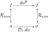
Figure 4. Verifying operations

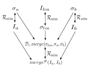
Figure 5. Verifying 3-way merge

Figure 4 considers the application of a data type operation (through the $do$ function) at a branch. Assuming that the simulation relation $\mathcal{R}_{sim}$ holds between the abstract state $I$ and the concrete state $\sigma$ at the branch, we would have to show that $\mathcal{R}_{sim}$ continues to hold after the application of the operation through the concrete $do$ function of the implementation and the abstract $do^{\#}$ function on the abstract state.

Figure 5 considers the application of a merge operation between branches $a$ and $b$. In this case, assuming $\mathcal{R}_{sim}$ between the abstract and concrete states at the two branches and for the LCA, we would then show that $\mathcal{R}_{sim}$ continues to hold between the concrete and abstract states obtained after merge. Note that since the concrete merge operation also uses the concrete LCA state $\sigma_{lca}$, we also assume that $\mathcal{R}_{sim}$ holds between the concrete and abstract LCA states.

Table 1. Store properties

$\Psi_{ts}(I)$	$\forall e,e^{\prime}\in I.E.\ e\xrightarrow{I.vis}e^{\prime}\Rightarrow I.time(e)<I.time(e^{\prime})$
	$\wedge\forall e,e^{\prime}\in I.E.\ I.time(e)=I.time(e^{\prime})\Rightarrow e=e^{\prime}$
$\Psi_{lca}(I_{l},I_{a},I_{b})$	$I_{l}.vis=I_{a}.vis_{\mid I_{l}.E}=I_{b}.vis_{\mid I_{l}.E}$
	$\wedge\forall e\in I_{l}.E.\ \forall e^{\prime}\in(I_{a}.E\cup I_{b}.E)\setminus I_{l}.E.\ e\xrightarrow{I_{a}.vis\cup I_{b}.vis}e^{\prime}$

These conditions consider the effect of concrete and abstract operations locally and thus enable automated verification. In order to discharge these conditions, we also consider two store properties, $\Psi_{ts}$ and $\Psi_{lca}$ that hold across all executions (shown in Table 1). $\Psi_{ts}$ pertains to the nature of the timestamps associated with each operation, while $\Psi_{lca}$ characterizes the lowest common ancestor used for merge. These properties hold naturally due to the semantics of the replicated store. These properties play an important role in discharging the conditions required for validity of the simulation relation.

In particular, $\Psi_{ts}(I)$ asserts that in the abstract state $I$, causally related events have increasing timestamps, and no two events have the same timestamp. $\Psi_{lca}(I_{l},I_{a},I_{b})$ will be instantiated with the LCA of two abstract states $I_{a}$ and $I_{b}$ (i.e. $I_{l}=lca^{\#}(I_{a},I_{b})$), and asserts that the visibility relation between events which are present in both $I_{a}$ and $I_{b}$ (and hence also in $I_{l}$) will be the same in all three abstract states. Further, every event in the LCA will be visible to newly added events in either of the two branches. These properties follow naturally from the definition of LCA and are also maintained by the store semantics.

Table 2 shows the conditions required for proving the validity of the simulation relation $\mathcal{R}_{sim}$. In particular, $\Phi_{do}$ and $\Phi_{merge}$ exactly encode the scenarios depicted in the figures 4 and 5. Note that for $\Phi_{do}$, we assume $\Psi_{ts}$ for the input abstract state on which the operation will be performed. Similarly, for $\Phi_{merge}$, we assume $\Psi_{ts}$ for all events in the merged abstract state (thus ensuring $\Psi_{ts}$ also holds for events in the original branches) and $\Psi_{lca}$ for the LCA of the abstract states.

Table 2. Sufficient conditions for showing validity of simulation relation

$\Phi_{do}(\mathcal{R}_{sim})$	$\forall I,\sigma,e,op,a,t.\ \mathcal{R}_{sim}(I,\sigma)\wedge do^{\#}(I,e,op,a,t)=I^{{}^{\prime}}$
	$\wedge~{}\mathcal{D}_{\tau}.do(op,\sigma,t)=(\sigma^{{}^{\prime}},a)\wedge\Psi_{ts}(I)\implies\mathcal{R}_{sim}(I^{{}^{\prime}},\sigma^{{}^{\prime}})$
$\Phi_{merge}(\mathcal{R}_{sim})$	$\forall I_{a},I_{b},\sigma_{a},\sigma_{b},\sigma_{lca}.\ \mathcal{R}_{sim}(I_{a},\sigma_{a})\wedge\mathcal{R}_{sim}(I_{b},\sigma_{b})$
	$\wedge~{}\mathcal{R}_{sim}(lca^{\#}(I_{a},I_{b}),\sigma_{lca})\wedge\Psi_{ts}(merge^{\#}(I_{a},I_{b}))\wedge\Psi_{lca}(lca^{\#}(I_{a},I_{b}),I_{a},I_{b})$
	$\implies\mathcal{R}_{sim}(merge^{\#}(I_{a},I_{b}),\mathcal{D}_{\tau}.merge(\sigma_{lca},\sigma_{a},\sigma_{b}))$
$\Phi_{spec}(\mathcal{R}_{sim})$	$\forall I,\sigma,e,op,a,t.\ \mathcal{R}_{sim}(I,\sigma)\wedge do^{\#}(I,e,op,a,t)=I^{{}^{\prime}}$
	$\wedge~{}\mathcal{D}_{\tau}.do(op,\sigma,t)=(\sigma^{{}^{\prime}},a)\wedge\Psi_{ts}(I)\implies a=\mathcal{F}_{\tau}(o,I)$
$\Phi_{con}(\mathcal{R}_{sim})$	$\forall I,\sigma_{a},\sigma_{b}.\ \mathcal{R}_{sim}(I,\sigma_{a})\wedge\mathcal{R}_{sim}(I,\sigma_{b})\implies\sigma_{a}\thicksim\sigma_{b}$

Once we show that the simulation relation is maintained at every transition in every execution inductively, we also have to show that it is strong enough to imply the data type specification as well as guarantee convergence. For this, we define two more conditions $\Phi_{spec}$ and $\Phi_{con}$ (also in table 2). $\Phi_{spec}$ says that if abstract state $I$ and concrete state $\sigma$ are related by $\mathcal{R}_{sim}$, then the return value of operation $o$ performed on $\sigma$ should match the value of the specification function $\mathcal{F}_{\tau}$ on the abstract state. Since the $\mathcal{R}_{sim}$ relation is maintained at every transition, if $\Phi_{spec}$ is valid, then the implementation will clearly satisfy the specification. Finally, for convergence, we require that if two concrete states are related to the same abstract state, then they should be observationally equivalent. This corresponds to our proposed notion of convergence modulo observable behavior.

Definition 4.1.

Given a MRDT implementation $\mathcal{D}_{\tau}$ of data type $\tau$, a replication-aware simulation relation $\mathcal{R}_{sim}\subseteq\mathcal{I}_{\tau}\times\Sigma$ is valid if $\Phi_{do}(\mathcal{R}_{sim})\wedge\Phi_{merge}(\mathcal{R}_{sim})\wedge\allowbreak\Phi_{spec}(\mathcal{R}_{sim})\allowbreak\wedge\allowbreak\Phi_{con}(\mathcal{R}_{sim})$.

Theorem 4.2 (Soundness).

Given a MRDT implementation $\mathcal{D}_{\tau}$ of data type $\tau$, if there exists a valid replication-aware simulation $\mathcal{R}_{sim}$, then the data type implementation $\mathcal{D}_{\tau}$ is correct .

4.2. Verifying OR-sets using simulation relations

Let us look at the simulation relations for verifying OR-set implementations in §2.1 against the specification $\mathcal{F}_{orset}$ in §2.2.1.

OR-set.

Following is a candidate valid simulation relation for the unoptimized OR-set from §2.1.1:

(3) $$\begin{split}\mathcal{R}_{sim}(I,\sigma)\iff(\forall(a,t)\in\sigma\iff\\ (\exists e\in I.E\wedge I.~{}oper(e)=add(a)\wedge I.time(e)=t~{}\wedge\\ \neg(\exists f\in I.E\wedge I.~{}oper(f)=remove(a)\wedge e\xrightarrow{vis}f)))\end{split}$$

The simulation relation says that for every pair of an element and a timestamp in the concrete state, there should be an $\mathsf{add}$ event in the abstract state which adds the element with the same timestamp, and there should not be a remove event of the same element which witnesses that add event. This simulation relation is maintained by all the set operations as well as by the merge operation, and it also matches the OR-set specification and guarantees convergence. We use F* to automatically discharge all the proof obligations of Table 2.

Space-efficient OR-set.

Following is a candidate valid simulation relation for the space-efficient OR-set (OR-set-space) from §2.1.2:

(4) $$\begin{split}\mathcal{R}_{sim}((E,oper,rval,time,vis),\sigma)\iff\\ (\forall(a,t)\in\sigma\implies(\exists e\in E.~{}oper(e)=add(a)\wedge time(e)=t\\ \wedge~{}\neg(\exists r\in E.~{}oper(r)=remove(a)\wedge e\xrightarrow{vis}r))~{}\wedge\\ (\forall e\in E.~{}oper(e)=add(a)\wedge\neg(\exists r\in E.oper(r)=remove(a)\\ \wedge~{}e\xrightarrow{vis}r)\implies t\geq time(e)))~{}\wedge\\ (\forall e\in E.\forall a\in\mathbb{N}.~{}oper(e)=add(a)\\ \wedge~{}\neg(\exists r\in E.~{}oper(r)=remove(a)\wedge e\xrightarrow{vis}r)\implies(a,\_)\in\sigma)\end{split}$$

The simulation relation in this case captures all the constraints of the one for OR-set with duplicates, but has additional constraints on the timestamp of the elements in the concrete state. In particular, for an element in the concrete state, the timestamp associated with that element will be the greatest timestamp of all the $\mathsf{add}$ events of the same element in the abstract state, which has not been witnessed by a $\mathsf{remove}$ event. Finally, we also need to capture the constraint in the abstract to concrete direction. If there is an $\mathsf{add}$ event not seen by a $\mathsf{remove}$ event on the same element, then the element is a member of the concrete state. As before, the proof obligations of Table 2 are through F*.

5. Composing MRDTs

A key benefit of our technique is that compound data types can be constructed by the composition of simpler data types through parametric polymorphism. The proofs of correctness of the compound data types can be constructed from the proofs of the underlying data types.

5.1. IRC-style chat

To illustrate the benefits of compositionality, we consider a decentralised IRC-like chat application with multiple channels. Each channel maintains the list of messages in reverse chronological order so that the most recent message may be displayed first. For simplicity, we assume that the channels are append-only; while new messages can be posted to the channels, old messages cannot be deleted. We also assume that while new channels may be created, existing channels may not be deleted.

1:$\mathcal{F}_{chat}(rd(ch),\langle E,oper,rval,time,vis\rangle)=log$ where

2:$\quad(\forall t,m.~{}(t,m)\in log\iff\exists e\in E.$

3:$\quad\qquad\qquad\qquad~{}oper(e)=send(ch,m)\wedge~{}time(e)=t)~{}\wedge$

4:$\quad(\forall t_{1},m_{1},t_{2},m_{2}.~{}ord~{}(t_{1},m_{1})~{}(t_{2},m_{2})~{}log$

5:$\quad\iff\exists e_{1},e_{2}\in E.~{}oper(e_{1})=send(ch,m_{1})~{}\wedge$

6:$\quad\qquad\qquad time(e_{1})=t_{1}~{}\wedge oper(e_{2})=send(ch,m_{2})~{}\wedge$

7:$\quad\qquad\qquad time(e_{2})=t_{2}\wedge t_{1}>t_{2})$

Figure 6. The specification of IRC-style chat.

The chat application supports sending a message to a channel and reading messages from a channel: $Op_{chat}=\{send(ch,m)\mid ch\in string\ ~{}\wedge~{}m\in string)\}~{}\cup~{}\{rd(ch)\allowbreak\mid ch\in string\}$. The specification of this chat application is given in Figure 6. For this we define a predicate $ord$ such that $ord(t_{1},m_{1})~{}(t_{2},m_{2})~{}l$ holds iff $t_{1}\neq t_{2}$ and $(t_{1},m_{1})$ occurs before $(t_{2},m_{2})$ in list $l$. The specification essentially says the log of messages contains all (and only those) messages that were sent, and messages are ordered in reverse chronological order.

Rather than implement this chat application from scratch, we may quite reasonably build it using existing MRDTs. We may use a MRDT map to store the association between the channel names and the list of messages. Given that the conversations take place in a decentralized manner, the list of messages in each channel should also be mergeable. For this purpose, we use a mergeable log, an MRDT list that totally orders the messages based on the message timestamp, to store the messages in each of the channels. As mentioned earlier, for simplicity we will assume that the map and the log are grow-only.

5.2. Mergeable log

1:$\mathcal{F}_{log}(rd,\langle E,oper,rval,time,vis\rangle)=lst$ where

2:$~{}\ (\forall t,m.~{}(t,m)\in lst\iff$

3:$~{}\ \qquad\exists e\in E.~{}oper(e)=append(m)~{}\wedge~{}time(e)=t)~{}\wedge$

4:$~{}\ (\forall t_{1},m_{1},t_{2},m_{2}.~{}ord~{}(t_{1},m_{1})~{}(t_{2},m_{2})~{}lst\iff$

5:$\quad\exists e_{1},e_{2}\in E.~{}oper(e_{1})=append(m_{1})~{}\wedge~{}time(e_{1})=t_{1}$

6:$\quad\wedge~{}oper(e_{2})=append(m_{2})~{}\wedge~{}time(e_{2})=t_{2}~{}\wedge~{}t_{1}>t_{2})$

7:

1:$\mathcal{D}_{log}=(\Sigma,\sigma_{0},do,merge_{log})\text{ where }$

2:$\quad\Sigma_{log}=\mathcal{P}(\mathbb{N}\times string)$

3:$\quad\sigma_{0}=\{\}$

4:$\quad do(append(m),\sigma,t)=((t,m)::\sigma,\bot)$

5:$\quad do(rd,\sigma,t)=(\sigma,\sigma)$

6:$\quad merge_{log}(\sigma_{lca},\sigma_{a},\sigma_{b})=$

7:$\quad\qquad sort((\sigma_{a}-\sigma_{lca})~{}@~{}(\sigma_{b}-\sigma_{lca}))~{}@~{}\sigma_{lca}$

8:

1:$\mathcal{R}_{sim-log}(I,\sigma)\iff$

2:$(\forall t,m.~{}(t,m)\in\sigma\iff$

3:$\quad\exists e\in I.E.~{}oper(e)=append(m)~{}\wedge~{}time(e)=t)~{}\wedge$

4:$\quad(\forall t_{1},m_{1},t_{2},m_{2}.~{}ord~{}(t_{1},m_{1})~{}(t_{2},m_{2})~{}\sigma\iff$

5:$\quad\exists e_{1},e_{2}\in I.E.~{}oper(e_{1})=append(m_{1})~{}\wedge~{}time(e_{1})=t_{1}$

6:$\quad\wedge~{}oper(e_{2})=append(m_{2})~{}\wedge~{}time(e_{2})=t_{2}~{}\wedge~{}t_{1}>t_{2})$

Figure 7. The specification, implementation and the simulation relation of mergeable log.

The mergeable log MRDT supports operations to append messages to the log and to read the log: $Op_{log}=\{rd\}\allowbreak~{}\cup~{}\allowbreak\{append(m)\mid m\in string\}$. The log maintains messages in reverse chronological order. Figure 7 presents the specification, implementation and the simulation relation of the mergeable log. The $sort$ function sorts the list in reverse chronological order based on the timestamps associated with the messages.

5.3. Generic map

1:$\mathcal{F}_{\alpha-map}(get(k,o_{\alpha}),I)=$

2:$\quad\text{let }I_{\alpha}=project(k,I)\text{ in }\mathcal{F}_{\alpha}(o_{\alpha},I_{\alpha})$

3:

1:$\mathcal{D}_{\alpha-map}=(\Sigma,\sigma_{0},do,merge_{\alpha-map})\text{ where }$

2:$\quad\Sigma_{\alpha-map}=\mathcal{P}(string\times\Sigma_{\alpha})$

3:$\quad\sigma_{0}=\{\}$

4:$\quad\delta(\sigma,k)=\begin{cases}\sigma(k),&\text{if}\ k\in dom(\sigma)\\ \sigma_{0_{\alpha}},&\text{otherwise}\end{cases}$

5:$\quad do(set(k,o_{\alpha}),\sigma,t)=$

6:$\quad\quad\text{let }(v,r)=do_{\alpha}(o_{\alpha},\delta(\sigma,k),t)\text{ in }(\sigma[k\mapsto v],r)$

7:$\quad do(get(k,o_{\alpha}),\sigma,t)=$

8:$\quad\quad\text{let }(\_,r)=do_{\alpha}(o_{\alpha},\delta(\sigma,k),t)\text{ in }(\sigma,r)$

9:$\quad merge_{\alpha-map}(\sigma_{lca},\sigma_{a},\sigma_{b})=$

10:$\quad\quad\{(k,v)\mid(k\in dom(\sigma_{lca})~{}\cup~{}dom(\sigma_{a})~{}\cup~{}dom(\sigma_{b}))~{}\wedge$

11:$\quad\quad\qquad\qquad v=merge_{\alpha}(\delta(\sigma_{lca},k),\delta(\sigma_{a},k),\delta(\sigma_{b},k))$

12:

1:$\mathcal{R}_{sim-\alpha-map}(I,\sigma)\iff\forall k.$

2:$(k\in dom(\sigma)\iff\exists e\in I.E.~{}oper(e)=set(k,\_))~{}\wedge$

3:$\quad\mathcal{R}_{sim-\alpha}~{}(project(k,I),~{}\delta(\sigma,k))$

Figure 8. The specification, implementation and simulation relation of $\alpha$-map.

We introduce a generic map MRDT, $\alpha$-map, which associates string keys with a value, where the value stored in the map is itself an MRDT. This $\alpha$-map is parameterised on an MRDT $\alpha$ and its implementation $\mathcal{D}_{\alpha}$, and supports $get$ and $set$ operations: $Op_{\alpha-map}=\{get(k,o_{\alpha})\mid k\in string\wedge o_{\alpha}\in Op_{\alpha}\}\cup\{set(k,o_{\alpha})\mid k\in string\wedge o_{\alpha}\in Op_{\alpha}\}$, where $Op_{\alpha}$ denotes the set of operations on the underlying value MRDT.

Figure 8 shows the specification, implementation and the simulation relation of $\alpha$-map. The implementations for get and $set$ operations both fetch the current value associated with the key $k$ (and the initial state of $\mathcal{D}_{\alpha}$ if the key is not present in the map), and apply the given operation $o_{\alpha}$ from the implementation $\mathcal{D}_{\alpha}$ on this value. While $set$ updates the binding in the map, $get$ does not do so and simply returns the value returned by $o_{\alpha}$. The merge operation merges the values for each key using the merge function of $\alpha$. The specification and simulation relation of $\alpha$-map use the specification and simulation relation of the underlying MRDT $\alpha$, by projecting the events associated with each key to an abstract execution of $\alpha$. We now provide the details of this projection function.

5.4. Projection function

1:$project~{}k~{}I_{\alpha-map}=I_{\alpha}\text{ where }$

2:$\quad I_{\alpha-map}=(\Sigma_{m},oper_{m},rval_{m},time_{m},vis_{m})$ and

3:$\quad I_{\alpha}=(\Sigma_{\alpha},oper_{\alpha},rval_{\alpha},time_{\alpha},vis_{\alpha})$ and

4: $(\forall e,k,o.~{}e\in\Sigma_{m}\wedge~{}oper_{m}(e)=set(k,o)\iff$

5:$\quad\exists e^{\prime}\in\Sigma_{\alpha}.~{}oper_{\alpha}(e^{\prime})=o~{}\wedge rval_{m}(e)=rval_{\alpha}(e^{\prime})~{}\wedge$

6:$\quad\quad~{}time_{m}(e)=time_{\alpha}(e^{\prime}))~{}\wedge$

7:$\quad(\forall e_{1},e_{2}.~{}e_{1}\in\Sigma_{m}\wedge e_{2}\in\Sigma_{m}\wedge~{}oper_{m}(e_{1})=set(k,\_)~{}\wedge$

8:$\quad oper_{m}(e_{2})=set(k,\_)~{}\wedge e_{1}\xrightarrow{vis_{m}}e_{2}\iff$

9:$\quad\exists e_{1}^{{}^{\prime}},e_{2}^{{}^{\prime}}\in\Sigma_{\alpha}.~{}time_{\alpha}(e_{1}^{{}^{\prime}})=time_{m}(e_{1})~{}\wedge$

10:$\quad\quad~{}time_{\alpha}(e_{2}^{{}^{\prime}})=time_{m}(e_{2})~{}\wedge e_{1}^{{}^{\prime}}\xrightarrow{vis_{\alpha}}e_{2}^{{}^{\prime}})$

Figure 9. Projection function for mapping $\alpha$-map execution to $\alpha$ execution.

Figure 9 gives the projection function which when given an abstract execution $I_{\alpha-map}$ of $\alpha$-map, projects all the $set$-events associated with a particular key $k$ to define an abstract execution $I_{\alpha}$. There is a one-to-one correspondence between $set$-events to $k$ in $I_{\alpha-map}$ and events in $I_{\alpha}$, with the corresponding events in $I_{\alpha}$ preserving the operation type, return values, timestamps and the visibility relation. The project function as used in the specification of $\mathcal{F}_{\alpha-map}$ ensures that the return value of $get$-events obey the specification $\mathcal{F}_{\alpha}$ as applied to the projected $\alpha$-execution.

Similarly, the simulation relation of $\alpha$-map requires the simulation relation of $\alpha$ to hold for every key, between the value associated with the key and the corresponding projected execution for the key. We can now verify the correctness of the generic $\alpha$-map MRDT by relying on the correctness of $\alpha$. That is, if $\mathcal{R}_{sim-\alpha}$ is a valid simulation relation for the implementation $\mathcal{D}_{\alpha}$, then $\mathcal{R}_{sim-\alpha-map}$ is a valid simulation relation for $\mathcal{D}_{\alpha-map}$. This allows us to build the proof of correctness of $\alpha$-map using the proof of correctness of $\alpha$.

1:$\mathcal{F}_{chat}(rd(ch),I)=\mathcal{F}_{log-map}(get(ch,rd),I)$

2:

3:$\mathcal{D}_{chat}=\mathcal{D}_{log-map}\text{ where }$

4:$\qquad do(send(ch,m),\sigma,t)=$

5:$\qquad\qquad do(set(ch,append(m)),\sigma,t)$

6:$\qquad do(rd(m),\sigma,t)=do(get(k,rd),\sigma,t)$

Figure 10. Implementation of IRC-style chat.

For our chat application, we instantiate $\alpha$-map with the mergeable log $\mathcal{D}_{log}$. The chat application itself is a wrapper around the log-map MRDT as shown in Fig. 10. In order to verify the correctness of $\mathcal{D}_{chat}$, we only need to separetely verify $\mathcal{D}_{\alpha-map}$ and $\mathcal{D}_{log}$. Note that one can instantiate $\alpha$ with any verified MRDT implementation to obtained a verified $\alpha$-map MRDT.

6. Case study: A Verified Queue MRDT

Okasaki (Okasaki, 1999) describes a purely functional queue with amortized time complexity of $O(1)$ for enqueue and dequeue operations. This queue is made up of two lists that hold the front and rear parts of the queue. Elements are enqueued to the rear queue and dequeued from the front queue (both are $O(1)$ operations). If the front queue is found to be empty at dequeue, then the rear queue is reversed and made to be the front queue ($O(n)$ operation). Since each element is part of exactly one reverse operation, the enqueue and the dequeue have an amortized time complexity of $O(1)$. In this section, we show how to convert this efficient sequential queue into an MRDT by providing additional semantics to handle concurrent operations.

For simplicity of specification, we tag each enqueued element with the unique timestamp of the enqueue operation, which ensures that all the elements in the queue are unique. The queue supports two operations: $Op_{queue}=\{dequeue\}\cup\{enqueue(a)\mid a\in\mathbb{V}\}$, where $\mathbb{V}$ is some value domain. Unlike a sequential queue, we follow an at-least-once dequeue semantics – an element inserted into the queue may be consumed by concurrent dequeues on different branches. At-least-once semantics is common for distributed queueing services such as Amazon Simple Queue Service(SQS) (Amazon, 2006) and RabbitMQ (RabbitMQ, 2007). At a merge, concurrent enqueues are ordered according to their timestamps.

6.1. Merge function of the replicated queue

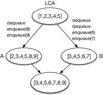
Figure 11. Three-way merge for queues

To illustrate the three-way merge function, consider the execution presented in figure 11. For simplicity, we assume that the timestamps are the same as the values enqueued. Starting from the LCA, each branch performs a sequence of dequeue and enqueue operations. The resulting versions are then merged. Observe that in the merged result, the elements 1 and 2 which were dequeued (with 1 dequeued on both the branches!) are not present. Elements 3, 4 and 5 which are present in all three versions are present in the merged result. Newly inserted elements appear at the suffix, sorted according to their timestamps.

The merge function first converts each of the queues to a list, and finds the longest common contiguous subsequence between the three versions ([3,4,5]). The newly enqueued elements are suffixes of this common subsequence – [8,9] and [6,7] in the queues A and B, respectively. The final merged result is obtained by appending the common subsequence to the suffixes merged according to their timestamps. Each of these operations has a time complexity of $O(n)$ where $n$ is the length of the longest list. Hence, the merge function is also an $O(n)$ operation .

6.2. Specification of the replicated queue

We now provide the specification for the queue MRDT, which is based on the declarative queue specification in Kartik et al. (Nagar et al., 2020). In particular, compared to the sequential queue, the only constraint that we relax is allowing multiple dequeues of the same element.

In order to describe the specification, we first introduce a number of axioms which declaratively specify different aspects of queue behaviour. Consider the $\mathsf{match}_{I}$ predicate defined for a pair of events $e_{1},e_{2}$ in an abstract execution $I$:

$$\mathsf{match}_{I}(e_{1},e_{2}) \Leftrightarrow I.oper(e_{1})=enqueue(a)$$

$$~{}~{}\wedge I.oper(e_{2})=dequeue\wedge a=I.rval(e_{2})$$

Let $\mathtt{EMPTY}$ be the value returned by a dequeue when the queue is empty. We define the following axioms:

• $AddRem(I)$ : $\forall e\in I.E.\ I.oper(e)=dequeue~{}\wedge$
  $I.rval(e)\neq\mathtt{EMPTY}\implies\exists e^{\prime}\in I.E.\ \mathsf{match}_{I}(e^{\prime},e)$

• $Empty(I)$ : $\forall e_{1},e_{2},e_{3}\in I.E.\ I.oper(e_{1})=dequeue~{}\wedge$
  $I.rval(e_{1})=\mathtt{EMPTY}~{}\wedge~{}I.oper(e_{2})=enqueue(a)~{}\wedge$
  $e_{2}\xrightarrow{I.vis}e_{1}\implies\exists e_{3}\in I.E.\ \mathsf{match}_{I}(e_{2},e_{3})\wedge e_{3}\xrightarrow{I.vis}e_{1}$

• $FIFO_{1}(I)$ : $\forall e_{1},e_{2},e_{3}\in I.E.\ I.oper(e_{1})=enqueue(a)~{}\wedge$
  $\mathsf{match}_{I}(e_{2},e_{3})~{}\wedge~{}e_{1}\xrightarrow{I.vis}e_{2}\implies\exists e_{4}\in I.E.\ \mathsf{match}_{I}(e_{1},e_{4})$

• $FIFO_{2}(I)$: $\forall e_{1},e_{2},e_{3},e_{4}\in I.E.\ \neg(\mathsf{match}_{I}(e_{1},e_{4})~{}\wedge$
  $\mathsf{match}_{I}(e_{2},e_{3})~{}\wedge~{}e_{1}\xrightarrow{I.vis}e_{2}~{}\wedge~{}e_{3}\xrightarrow{I.vis}e_{4})$

These axioms essentially encode queue semantics. $AddRem$ says that for every dequeue event which does not return $\mathtt{EMPTY}$, there must exist a matching enqueue event. $Empty$ says that if a dequeue event returns $\mathtt{EMPTY}$, there should not be an unmatched enqueue visible to it. Finally, $FIFO_{1}$ and $FIFO_{2}$ encode the first-in-first-out nature of the queue. These axioms ensure that if an enqueue event $e_{1}$ was visible to another enqueue event $e_{2}$, then the element inserted by $e_{1}$ will be dequeued first. Notice that sequential queue would also have an injectivity axiom, which disallows multiple dequeues to be matched to an enqueue, but we do not enforce this requirement for the replicated queue.

To define $\mathcal{F}_{Queue}$, we first note that enqueue operation always returns $\bot$. For an abstract state $I$, $\mathcal{F}_{Queue}(dequeue,I)$ returns $a$ such that if we add the new event $e$ for the dequeue to the abstract state $I$, then the resulting abstract state $do^{\#}(I,e,dequeue,a,t)$ must satisfy all the queue axioms.

Notice how the queue axioms are substantially different from the way the MRDT queue is actually implemented. The simulation relation that we use to bridge this gap and relate the implementation with the abstract state is actually very straightforward: we simply say that for every element present in the concrete state of the queue, there must be an enqueue event without a matching dequeue. We also assert the other direction, and enforce the queue axioms on the abstract state. The complete simulation relation can be found in the supplemental material. We were able to successfully discharge the conditions for validity of the simulation relation using F*.

7. Evaluation

In this section, we evaluate the instantiation of the formalism developed thus far in Peepul, an F* library of certified efficient MRDTs. We first discuss the verification effort followed by the performance evaluation of efficient MRDTs compared to existing work. These results were obtained on a 2-socket Intel®Xeon®Gold 5120 x86-64 (Intel Xeon Gold 5120, 2020) server running Ubuntu 18.04 with 64GB of main memory.

7.1. Verification in F*

F*’s core is a functional programming language inspired by ML, with support for program verification using refinement types and monadic effects. Though F* has support for built-in effects, Peepul library only uses the pure fragment of the language. Given that we can extract OCaml code from our verified implementations in F*, we are able to directly utilise our MRDTs on top of Irmin (Irmin, 2021), a Git-like distributed database, whose execution model fits the MRDT system model.

As part of the Peepul library, we have implemented and verified 9 MRDTs – increment-only counter, PN counter, enable-wins flag, last-writer-wins register, grows-only set, grows-only map, mergeable log, observed-remove set and functional queue. Our specifications capture both the functional correctness of local operations as well as the semantics of the concurrent conflicting operations.

F*’s support for type classes provides a modular way to implement and verify MRDTs. The Peepul library defines a MRDT type class that captures the sufficient conditions to be proved for each MRDT as given in Table 2. This library contains 124 lines of F* code. Each MRDT is a specific instance of the type class which satisfy the conditions. It is useful to note that our MRDTs sets, maps and queues are polymorphic in their contents and may be plugged with other MRDTs to construct more complex MRDTs as seen in §5.

Table 3. Peepul verification effort.

MRDTs verified	#Lines code	#Lines proof	#Lemmas	Verif. time (s)
Increment-only counter	6	43	2	3.494
PN counter	8	43	2	23.211
Enable-wins flag	20	58	3	1074
		81	6	171
		89	7	104
LWW register	5	44	1	4.21
G-set	10	23	0	4.71
		28	1	2.462
		33	2	1.993
G-map	48	26	0	26.089
Mergeable log	39	95	2	36.562
OR-set (§2.1.1)	30	36	0	43.85
		41	1	21.656
		46	2	8.829
OR-set-space (§2.1.2)	59	108	7	1716
OR-set-spacetime	97	266	7	1854
Queue	32	1123	75	4753

Table 3 tabulates the verification effort for each MRDT in the Peepul library. We include three versions of OR-sets:

• OR-set: the unoptimized one from §2.1.1 which uses a list for storing the elements and contains duplicates.

• OR-set-space: the space-optimized one from §2.1.2 which also uses a list but does not have duplicates.

• OR-set-spacetime: a space- and time-optimized one which uses a binary search tree for storing the elements and has no duplicates. The merge function produces a height balanced binary tree.

The lines of code represents the number of lines for implementing the data structure without counting the lines for refinements, lemmas, theorems and proofs. This is approximately the number of lines of code there will be if the data structures were implemented in OCaml. Everything else that has to do with verification is included in the lines of proofs. It is useful to note that the lines of proof for simple MRDTs such as counter and last-writer-wins (LWW) register is high compared to the lines of code since we also specify and prove their full functional correctness.

For many of the proofs, F* is able to automatically verify the properties either without any lemmas or just a few, thanks to F* discharging the proof obligations to the SMT solver. Most of the proofs are a few tens of lines of code with the exception of queues. In queues, the implementation is far removed from the specification, and hence, additional lemmas were necessary to bridge this gap.

F* allows the user to provide additional lemmas that help the solver arrive to the proof faster. We illustrate this for enable-wins flag, G-set and OR-set by adding additional lemmas. Correspondingly, we observe that the verification time reduces significantly. Thanks to F*, the developers of new MRDTs in Peepul can strike a balance between verification times and manual verification effort.

In this work, we have not used F* support for tactics and interactive proofs. We believe that some of the time consuming calls to the SMT solver may be profitably replaced by a few interactive proofs. On the whole, the choice of F* for Peepul reduces manual effort and most of the proofs are checked within few seconds.

7.2. Performance evaluation

In this section, we evaluate the runtime performance of efficient MRDTs in Peepul.

7.2.1. Peepul vs Quark

We first compare the performance of Peepul MRDTs against the MRDTs presented in Kaki et al. (Kaki et al., 2019) (Quark). Recall that Quark lifts sequential data types to MRDTs by equipping them with a merge function, which converts the concrete state of the MRDT to a relational (set-based) representation that captures the characteristic relations of the data type. The actual merge is implemented as a merge of these sets for each of the characteristic relations. After merge of the relational representations, the final result is obtained by a concretization function. Compared to this, Peepul merges are implemented directly on the concrete representations.

To highlight the impact of the efficient merge function in Peepul, we evaluate the performance of merge in queues. Both Peepul and Quark uses the same sequential queue representation, and the only difference is the merge function between the two. For this experiment, we start with an empty queue, and perform a series of randomly generated operations with 75:25 split between enqueues and dequeues. We use this version as the LCA and subsequently perform two different sets of operations to get the two divergent versions. We then merge these versions to measure the time taken for the merge.

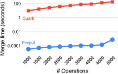
Figure 12. Merge performance of Peepul and Quark queues.

The results are reported in figure 12. For a queue, Quark needs to reify the ordering relation as a set which will contain $n^{2}$ elements for a queue of size $n$. In addition, there is also the cost of abstracting and concretising the queue to and from relational representation. As a result, the merge function takes 10 seconds for 1000 operations, increasing to 178 seconds for 5000 operations. On the other hand, Peepul’s linear-time merge took less than a millisecond in all of the cases. This shows the that Quark merge is unacceptably slow even reasonably sized queues, while Peepul remains fast and practical.

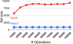
Figure 13. Performance of Peepul and Quark OR-sets.

We also compare the performance of OR-set in Peepul and Quark. Since the merge function in Quark is based on automatic relational reification, Quark does not allow duplicate elements to be removed from the OR-set. To highlight the impact of duplicate elements, we perform an experiment similar to the queue one except that we pick a 50:50 split between add and remove operations. The values added are randomly picked in the range (0:1000). For Peepul, we pick the space-optimized OR-set (OR-set-space). We report the number of elements in the final set including duplicates.

The results are presented in figure 13. Due to the duplicates, the size of the Quark set increases with increasing number of operations; the growth is not linear due to the stochastic interplay between add and remove. For Peepul, the set size always remains below 1000 which is the range of the values picked. The results show that MRDTs in Peepul are much more efficient than in Quark.

7.2.2. Peepul OR-set performance

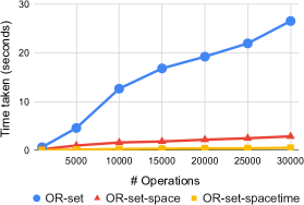
Figure 14. Running time of OR-sets.

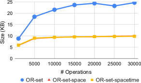
Figure 15. Space consumption of OR-sets. The OR-set-space line is hidden by the OR-set-spacetime line.

We also compare the overall performance of the three OR-set implementations in Peepul. Our workload consists of 70% lookups, 20% adds and 10% remove operations starting from an initial empty set on two different branches. We trigger a merge every 500 operations. We measure the overall execution time for the entire workload and the maximum size of the set during the execution.

The results are reported in figures 14 and 15. The results show that OR-set-spacetime is the fastest, and is around 5$\times$ faster than OR-set-space due to the fast reads and writes thanks to the binary search tree in OR-set-spacetime. Both OR-set-space and OR-set-spacetime consume similar amount of memory. The unoptimized OR-set is both slower and consumes more memory than the other variants due to the duplicates. The results show that Peepul enables construction of efficient certified MRDTs that have significant performance benefits compared to unoptimised ones.

8. Related Work

Reconciling concurrent updates is an important problem in distributed systems. Some of the works proposing new designs and implementations of RDTs (Shapiro et al., 2011; Roh et al., 2011; Bieniusa et al., 2012) neither provide their formal specification nor verify them. Due to the concurrently evolving state of the replicas, informally reasoning about the correctness of even simple RDTs is tedious and error prone. In this work, our focus is on mechanically verifying efficient implementations of MRDTs.

There are several works that focus on specification and verification of CRDTs (Burckhardt et al., 2014; Liu et al., 2020; Zeller et al., 2014; Nair et al., 2020; Attiya et al., 2016; Gomes et al., 2017; Nagar and Jagannathan, 2019). CRDTs typically assume a system model which involves several replicas communicating over network with asynchronous message passing. Correspondingly, the specification and verification techniques for CRDTs will have to take into account of the properties of message passing such as message ordering and delivery guarantees. On the other hand, MRDTs are described over a Git-like distributed store with branching and merging, which in turn may be implemented over asynchronous message passing. We believe that, by lifting the level of abstraction, MRDTs are easy to specify, implement and verify compared to CRDTs.

In terms of mechanised verification of RDTs, prior work has used both automated and interactive verification. Zeller et al. (Zeller et al., 2014) verify state-based CRDTs with the help of interactive theorem prover Isabelle/HOL. Gomes et al. (Gomes et al., 2017) develop a foundational framework for proving the correctness of operation-based CRDTs. In particular, they construct a formal network model that may delay, drop or reorder messages sent between replicas. Under these assumptions, they verify several op-based CRDTs using Isabelle/HOL. Nair et al. (Nair et al., 2020) presents an SMT-based verification tool to specify state-based CRDTs and verify invariants over its state. Kartik et al. (Nagar and Jagannathan, 2019) also utilise SMT-solver to automatically verify the convergence of CRDTs under different weak consistency policies. Liu et al. (Liu et al., 2020) present an extension of the SMT-solver-aided Liquid Haskell to allow refinement types on type classes and use to implement a framework to verify operation-based CRDTs. Similar to Liu et al., Peepul also uses an SMT-solver-aided programming language F*. We find that SMT-solver-aided programming language offers a useful trade off between manual verification effort and verification time.

Our verification framework for MRDTs builds on the concept of replication-aware simulation introduced by Burckhardt et al. (Burckhardt et al., 2014). Burckhardt et al. present precise specifications for RDTs and (non-mechanized) proof of correctness for a few CRDT implementations. Burckhardt et al.’s specifications are presented over the CRDT system model with explicit message passing between replicas. In this work, we lift these specifications to a higher level by abstracting out the guarantees provided by the low-level store ($\Psi_{ts}$ and $\Psi_{lca}$). Further, we also observe that the simulation relation $\mathcal{R}_{sim}$ cannot be used as an inductive invariant on its own, and instead, a conjunction of $\mathcal{R}_{sim}$ with $\Psi_{ts}$ and $\Psi_{lca}$ is required (see conditions $\Phi_{do}$ and $\Phi_{merge}$ in Table 2). In order to enable mechanised verification, we identify the relationship between $\mathcal{R}_{sim}$ and the functional correctness and convergence of MRDTs. This leads to a formal specification framework that is suitable for mechanized and automated verification. We demonstrate this by successfully verifying a number of complex MRDT implementations in F* including the first, formally verified replicated queue.

MRDTs were first introduced by Farnier et al. (Farinier et al., 2015) for Irmin (Irmin, 2021), a distributed database built on the principles of Git. Quark (Kaki et al., 2019) automatically derives merge functions for MRDTs using invertible relational specification. However, their merge semantics focused only on convergence, and not the functional correctness of the data type. Our evaluation (§7.2.1) shows that merges through automatically derived invertible relational specification is prohibitively expensive for data types with rich structure such as queues. Tardis (Crooks et al., 2016) also uses branch-and-merge approach to weak consistency, but does not focus on verifying the correctness of the RDTs.

Not all application logic can be expressed only using eventually consistent and convergent RDTs. For example, a replicated bank account which guarantees non-negative balance requires coordination between concurrent withdraw operations. Several previous works have explored RDTs that utilize on-demand coordination based on application invariants (Sivaramakrishnan et al., 2015; Gotsman et al., 2016; Kaki et al., 2018; Najafzadeh et al., 2016; Houshmand and Lesani, 2019; De Porre et al., 2021). We leave the challenge of extending Peepul to support on-demand coordination to future work.

Appendix

Appendix A Proof of Theorem 4.2

Theorem 4.2. Given a MRDT implementation $\mathcal{D}_{\tau}$ of data type $\tau$, if there exists a valid replication-aware simulation $\mathcal{R}_{sim}$, then the data type implementation $\mathcal{D}_{\tau}$ is correct.

Proof.

We first show that for all executions $\chi$ of the store LTS $\mathcal{M}_{D_{\tau}}$, $\mathcal{R}_{sim}$ holds at every transition. At every step, we will also show that the return value of every operation obeys the data-type specification and convergence modulo observable behavior is satisfied. The proof is by induction on the length of the execution.

BASE CASE:
Consider that the labelled transition system is in the initial state $C_{\bot}=(\phi_{\bot},\delta_{\bot},0)$ with only one branch $b_{\bot}$.
$\chi=(\phi_{\bot},\delta_{\bot},0)$
To prove:
$\mathcal{R}_{sim}(\delta(b_{\tau}),\phi(b_{\tau}))\implies(\chi\models\mathcal{F}_{\tau}$ and $\chi$ is convergent modulo observable behavior).

Proof:
For every operation o of $\tau$, let
$(\phi_{\bot},\delta_{\bot},0)\xrightarrow{DO(o,b_{\bot})}(\phi^{{}^{\prime}},\delta^{{}^{\prime}},1)$
Then according to $\Phi_{spec}(\mathcal{R}_{sim})$ in Table 2,

(5) $$\mathcal{R}_{sim}(\delta_{\bot}(b_{\bot}),\phi_{\bot}(b_{\bot}))\wedge do^{\#}(\delta_{\bot}(b_{\bot}),e,o,a,0)=I^{{}^{\prime}}\wedge$$

$$\mathcal{D}_{\tau}.do(o,\phi_{\bot}(b_{\bot}),0)=(\phi^{{}^{\prime}}(b_{\bot}),a)\wedge\Psi_{ts}(\delta_{\bot}(b_{\bot}))\implies$$

$$a=\mathcal{F}_{\tau}(o,\delta_{\bot}(b_{\bot}))$$

which is the necessary condition for $\chi\models\mathcal{F}_{\tau}$.

The condition for eq (2) in Section. 3 is also satisfied, since there is only one branch $b_{\bot}$ in the execution. Hence $\chi$ is convergent modulo observable behavior. Thus the base case is proved.

INDUCTIVE CASE:
Consider an execution
$\chi=(\phi_{\bot},\delta_{\bot},0)\xrightarrow{e_{1}}(\phi_{1},\delta_{1},t_{1})\xrightarrow{e_{2}}\dots\xrightarrow{e_{n}}(\phi_{n},\delta_{n},t_{n})$.
To prove:
For an execution $\chi$, if $\chi\models\mathcal{F}_{\tau}$ and $\chi$ is convergent modulo observable behavior, then on applying a single step of the store execution, the new execution obtained $\chi^{{}^{\prime}}$, satisfies the specification and is convergent modulo observable behavior.

Proof ($\chi^{{}^{\prime}}\models\mathcal{F}_{\tau}$):
We prove it by case-analysis on labels in the labelled transition system.
Case 1:
The first case is the label being CREATEBRANCH.
$(\phi_{n},\delta_{n},t)\xrightarrow{CREATEBRANCH(b_{1},b_{2})}(\phi_{n+1},\delta_{n+1},t)$
$\phi_{n+1}=\phi_{n}[b_{2}\mapsto\phi_{n}(b_{1})]\hskip 28.45274pt\delta_{n+1}=\delta_{n}[b_{2}\mapsto\delta_{n}(b_{1})]$
$\chi^{{}^{\prime}}=\chi\xrightarrow{CREATEBRANCH(b_{1},b_{2})}(\phi_{n+1},\delta_{n+1},t)$
We need to prove that $\chi^{{}^{\prime}}\models\mathcal{F}_{\tau}$.
For every operation o, of the data type, let
$(\phi_{n+1},\delta_{n+1},t)\xrightarrow{DO(o,b)}(\phi_{n+2},\delta_{n+2},t+1)$
Then according to $\Phi_{spec}(\mathcal{R}_{sim})$ in Table 2,

(6) $$\mathcal{R}_{sim}(\delta_{n+1}(b),\phi_{n+1}(b))\wedge do^{\#}(\delta_{n+1}(b),e,o,a,t)=I^{{}^{\prime}}\wedge$$

$$\mathcal{D}_{\tau}.do(o,\phi_{n+1}(b),t)=(\phi_{n+2}(b),a)\wedge\Psi_{ts}(\delta_{n+1}(b))\implies$$

$$a=\mathcal{F}_{\tau}(o,\phi_{n+1}(b))$$

which is the necessary condition for $\chi^{{}^{\prime}}\models\mathcal{F}_{\tau}$.

Case 2:
The second case is the label being DO.
$(\phi_{n},\delta_{n},t)\xrightarrow{DO(o,b)}(\phi_{n+1},\delta_{n+1},t+1)$
$\chi^{{}^{\prime}}=\chi\xrightarrow{DO(o,b)}(\phi_{n+1},\delta_{n+1},t+1)$
We need to prove that $\chi^{{}^{\prime}}\models\mathcal{F}_{\tau}$.
For every operation o, of the data type, let
$(\phi_{n+1},\delta_{n+1},t+1)\xrightarrow{DO(o,b)}(\phi_{n+2},\delta_{n+2},t+2)$
Then according to $\Phi_{spec}(\mathcal{R}_{sim})$ in Table 2,

(7) $$\mathcal{R}_{sim}(\delta_{n+1}(b),\phi_{n+1}(b))\wedge do^{\#}(\delta_{n+1}(b),e,o,a,t+1)=I^{{}^{\prime}}\wedge$$

$$\mathcal{D}_{\tau}.do(o,\phi_{n+1}(b),t+1)=(\phi_{n+2}(b),a)\wedge\Psi_{ts}(\delta_{n+1}(b))\implies$$

$$a=\mathcal{F}_{\tau}(o,\phi_{n+1}(b))$$

which is the necessary condition for $\chi^{{}^{\prime}}\models\mathcal{F}_{\tau}$.

Case 3:
The second case is the label being MERGE.
$(\phi_{n},\delta_{n},t)\xrightarrow{MERGE(b_{1},b_{2})}(\phi_{n+1},\delta_{n+1},t)$
$\chi^{{}^{\prime}}=\chi\xrightarrow{MERGE(b_{1},b_{2})}(\phi_{n+1},\delta_{n+1},t)$
We need to prove that $\chi^{{}^{\prime}}\models\mathcal{F}_{\tau}$.
For every operation o, of the data type, let
$(\phi_{n+1},\delta_{n+1},t)\xrightarrow{MERGE(b_{1},b_{2})}(\phi_{n+2},\delta_{n+2},t+1)$
Then according to $\Phi_{spec}(\mathcal{R}_{sim})$ in Table 2,

(8) $$\mathcal{R}_{sim}(\delta_{n+1}(b),\phi_{n+1}(b))\wedge do^{\#}(\delta_{n+1}(b),e,o,a,t)=I^{{}^{\prime}}\wedge$$

$$\mathcal{D}_{\tau}.do(o,\phi_{n+1}(b),t)=(\phi_{n+2}(b),a)\wedge\Psi_{ts}(\delta_{n+1}(b))\implies$$

$$a=\mathcal{F}_{\tau}(o,\phi_{n+1}(b))$$

which is the necessary condition for $\chi^{{}^{\prime}}\models\mathcal{F}_{\tau}$.

Proof ($\chi^{{}^{\prime}}$ is convergent modulo observable behavior):
Let $\chi^{{}^{\prime}}$ be the execution obtained after applying any of the transitions (CREATEBRANCH, DO, MERGE) to $\chi$. For proving $\chi^{{}^{\prime}}$ is convergent modulo observable behavior, we need to show,

(9) $$\forall b_{1},b_{2}\in dom(\phi_{i}).\delta_{i}(b_{1})=\delta_{i}(b_{2})\implies\phi_{i}(b_{1})\thicksim\phi_{i}(b_{2})$$

We know that there is a valid simulation relation between $\mathcal{D}_{\tau}$ and $\mathcal{F}_{\tau}$.

(10) $$\forall b_{1},b_{2}\in dom(\phi_{i}).\mathcal{R}_{sim}(\delta_{i}(b_{1}),\phi_{i}(b_{1}))\wedge$$

$$\mathcal{R}_{sim}(\delta_{i}(b_{2}),\phi_{i}(b_{2}))$$

On substituting $\delta_{i}(b_{1})$ for $\delta_{i}(b_{2})$ according to ( 9) in ( 10) we get,
$\forall b_{1},b_{2}\in dom(\phi_{i}).\mathcal{R}_{sim}(\delta_{i}(b_{1}),\phi_{i}(b_{1}))\wedge\\ \mathcal{R}_{sim}(\delta_{i}(b_{2}),\phi_{i}(b_{2}))\\ \implies\mathcal{R}_{sim}(\delta_{i}(b_{1}),\phi_{i}(b_{1}))\wedge\mathcal{R}_{sim}(\delta_{i}(b_{1}),\phi_{i}(b_{2}))$

According to $\Phi_{con}(\mathcal{R}_{sim})$ in Table 2,
$\mathcal{R}_{sim}(\delta_{i}(b_{1}),\phi_{i}(b_{1}))\wedge\mathcal{R}_{sim}(\delta_{i}(b_{1}),\phi_{i}(b_{2}))\\ \implies\phi_{i}(b_{1})\thicksim\phi_{i}(b_{2})$
Hence $\chi^{{}^{\prime}}$ is convergent modulo observable behavior.

∎

Appendix B Functional queue simulation relation and implementation

B.1. Simulation relation

Consider the $match$ predicate as defined in Section 5.1:

(11) $$\begin{split}{match}_{I}(e_{1},e_{2})&\Leftrightarrow I.oper(e_{1})=enqueue(a)\\ &\wedge I.oper(e_{2})=dequeue\wedge a=I.rval(e_{2})\end{split}$$

We define the simulation relation, $\mathcal{R}_{sim}$ for an abstract state $I$ and a concrete state $\sigma$ as follows:

(12) $$\begin{split}\mathcal{R}_{sim}(I,\sigma)\iff((\forall(a,t)\in\sigma\iff\\ (\exists e\in I.E\wedge I.oper(e)=enqueue(a)\wedge I.time(e)=t\wedge\\ \neg(\exists d\in I.E\wedge{match}_{I}(e,d)\wedge e\xrightarrow{vis}d)))\wedge\\ (\forall(a_{1},t_{1})(a_{2},t_{2})\in\sigma\wedge{order}_{\sigma}(a_{1},t_{1})(a_{2},t_{2})\iff\\ ((\exists e_{1}e_{2}\in I.E\wedge I.oper(e_{1})=enqueue(a_{1})\wedge\\ I.oper(e_{2})=enqueue(a_{2})\wedge I.time(e_{1})=t_{1}\wedge I.time(e_{2})=t_{2}\\ \neg(\exists d\in I.E\wedge(({match}_{I}(e_{1},d)\wedge e_{1}\xrightarrow{vis}d)\vee\\ ({match}_{I}(e_{2},d)\wedge e_{2}\xrightarrow{vis}d)))\wedge\\ (e_{1}\xrightarrow{vis}e_{2}\vee(\neg(e_{1}{\xrightarrow{vis}}e_{2}\vee e_{2}{\xrightarrow{vis}}e_{1})\wedge t_{1}<t_{2}))))))\end{split}$$

where ${order}_{\sigma}$ $x_{1}$ $x_{2}$ is the predicate that states $x_{1}$ occurs before $x_{2}$ in the concrete state $\sigma$.

The simulation relation $\mathcal{R}_{sim}$ consists of two parts. The first part states that for any element $a$ in the concrete state of the queue, there exists an enqueue operation, $e$ in the abstract state, that is not matched with any dequeue operation, and the converse of this. The second part of the relation states that for any two elements $a_{1}$ and $a_{2}$ in the concrete state of the queue, such that $a_{1}$ occurs before $a_{2}$, there exist two enqueue operations, $e_{1}$ and $e_{2}$ in the abstract state, that are not matched with any dequeue operation, such that $e_{1}\xrightarrow{vis}e_{2}$ ($e_{2}$ was performed after $e_{1}$) or $(\neg(e_{1}{\xrightarrow{vis}}e_{2}$ $\vee$ $e_{2}{\xrightarrow{vis}}e_{1})$ $\wedge$ $t_{1}<t_{2})$ ($e_{1}$ and $e_{2}$ are concurrent operations), and the converse of this. The first part takes care of the membership of the elements in the queue, while the second part takes care of the ordering of the elements in the queue.

B.2. Functional queue implementation

The definition of the state of the functional queue is as follows:

⬇

type s =

| S of (int * int) list *

(int * int) list

The enqueue and dequeue functions for the functional queue are defined as follows:

⬇

let enqueue x q =

(S q.front (x::q.back))

⬇

let norm q =

match q with

|(S [] back) -> (S (rev back) [])

|_ -> q

⬇

let dequeue q =

match q with

|(S [] []) -> (None, q)

|(S (x::xs) _) -> (Some x, (S xs q.back))

|(S [] (x::xs)) ->

let (S (y::ys) []) = norm q in

(Some y, (S ys []))

Following are the definitions of some functions used as helper functions for the three-way merge. In all of these definitions, the first element of the pair is taken to be the timestamp, and the second element to be the actual enqueued element. union1 is used to merge two lists of pairs (with unique first elements) that are sorted according to the first element of the pair:

⬇

let rec union l1 l2 =

match l1, l2 with

| [], [] -> []

| [], l2 -> l2

| l1, [] -> l1

| h1::t1, h2::t2 -> if (fst h1 < fst h2)

then h1::(union t1 l2)

else h2::(union l1 t2)

diff_s is used to find the difference between two lists of pairs with unique first elements, that are sorted according to the first element of the pair. Additionally, in the context where diff_s is used, a is a child of l. This function is used to find the newly enqueued elements in a. This simplifies the function to finding the longest contiguous subsequence that is present in a but not l. This also can be interpreted as finding the longest suffix of a that is not present in l, since all the newly enqueued elements occur after the existing elements. This task can be completed in $O(n)$ time where $n$ is the length of the longest of the two lists.

⬇

let rec diff_s a l =

match a, l with

| x::xs, y::ys -> if (fst y) < (fst x)

then diff_s (x::xs) ys else (diff_s xs ys)

| [], y::ys -> []

| _, [] -> a

intersection is used to find the longest common contiguous subsequence between l, a and b. Again, in the context where intersection is used, a and b are children of l. This finds the list of elements that have not been dequeued in either a or b. Hence, the problem is simplified to finding the longest contiguous subsequence of l that is a prefix of a and b. Since all the three lists are sorted according to the first element of the pair, this task can be completed in $O(n)$ time where $n$ is the length of the longest of the three lists.

⬇

let rec intersection l a b =

match l, a, b with

| x::xs, y::ys, z::zs ->

if ((fst x) < (fst y)

|| (fst x) < (fst z)) then

(intersection xs (y::ys) (z::zs))

else (x::(intersection xs ys zs))

| x::xs, [], z::zs -> []

| x::xs, y::ys, [] -> []

| x::xs, [], [] -> []

| [], _, _ -> []

tolist is used to convert a functional queue to a single list. This function takes $O(n)$ time where $n$ is the length of the functional queue.

⬇

let tolist (S f b) = append f (rev b)

For the three-way merge between l, a and b, we first find the elements that are not dequeued in a or b. Then we find the list of newly enqueued elements in a and b, and append it to the list of undequeued elements. The core of the three-way merge is defined as follows:

⬇

let merge_s l a b =

let ixn = intersection l a b in

let diff_a = diff_s a l in

let diff_b = diff_s b l in

let union_ab = union diff_a diff_b in

append ixn union_ab

The three-way merge for l, a and b is defined as follows:

⬇

let merge l a b =

(S

(merge_s (tolist l) (tolist a) (tolist b))

[])

Since all the tasks involved in merge take linear time in terms of the length of the longest list, which is equal to that of the longest queue, merge takes $O(n)$ time where $n$ is the length of the longest queue.