Automated Progressive Learning for Efficient Training of Vision Transformers

Abstract

Recent advances in vision Transformers (ViTs) have come with a voracious appetite for computing power, highlighting the urgent need to develop efficient training methods for ViTs. Progressive learning, a training scheme where the model capacity grows progressively during training, has started showing its ability in efficient training. In this paper, we take a practical step towards efficient training of ViTs by customizing and automating progressive learning. First, we develop a strong manual baseline for progressive learning of ViTs, by introducing momentum growth (MoGrow) to bridge the gap brought by model growth. Then, we propose automated progressive learning (AutoProg), an efficient training scheme that aims to achieve lossless acceleration by automatically increasing the training overload on-the-fly; this is achieved by adaptively deciding whether, where and how much should the model grow during progressive learning. Specifically, we first relax the optimization of the growth schedule to sub-network architecture optimization problem, then propose one-shot estimation of the sub-network performance via an elastic supernet. The searching overhead is reduced to minimal by recycling the parameters of the supernet. Extensive experiments of efficient training on ImageNet with two representative ViT models, DeiT and VOLO, demonstrate that AutoProg can accelerate ViTs training by up to 85.1% with no performance drop.

1 Introduction

With powerful high model capacity and large amounts of data, Transformers have dramatically improved the performance on many tasks in computer vision (CV) [72, 56]. The pioneering ViT model [21], scales the model size to 1,021 billion FLOPs, 250$\times$ larger than ResNet-50 [31]. Through pre-training on the large-scale JFT-3B dataset [90], the recently proposed ViT model, CoAtNet [15], reached state-of-the-art performance, with about 8$\times$ training cost of the original ViT. The rapid growth in training scale inevitably leads to higher computation cost and carbon emissions. As shown in Tab. 1, recent breakthroughs of vision Transformers have come with a voracious appetite for computing power, resulting in considerable growth of environmental costs. Thus, it becomes extremely important to make ViTs training tenable in computation and energy consumption.

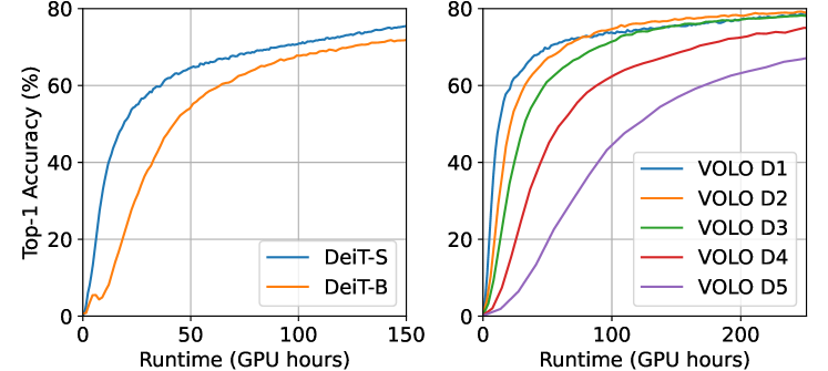
Figure 1: Accuracy of ViTs (DeiT [72] and VOLO [88]) during training. Smaller ViTs converge faster in terms of runtime. Models in the legend are sorted in increasing order of model size.

Model	CO2e (lbs)	ImageNet Acc. (%)
ResNet-50 [31, 21]	267	77.54
BERTbase [18]	1,438	-
Avg person per year [65]	11,023	-
ViT-H/14 [21]	22,793	88.55
CoAtNet [15]	183,256	90.88

Table 1: The growth in training scale of vision models results in considerable growth of environmental costs. The CO₂e of human life and a language model, BERT [18] are also included for comparison. The results of ResNet-50, ViT-H/14 are from [21], and trained on JFT-300M [66]. CoAtNet is trained on JFT-3B [90].

In mainstream deep learning training schemes, all the network parameters participate in every training iteration. However, we empirically found that training only a small part of the parameters yields comparable performance in early training stages of ViTs. As shown in Footnote 3, smaller ViTs converge much faster in terms of runtime (though they would be eventually surpassed given enough training time). The above observation motivates us to rethink the efficiency bottlenecks of training ViTs: does every parameter, every input element need to participate in all the training steps?

Here, we make the Growing Ticket Hypothesis of ViTs: the performance of a large ViT model, can be reached by first training its sub-network, then the full network after properly growing, with the same total training iterations. This hypothesis generalizes the lottery ticket hypothesis [24] by adding a finetuning procedure at the full model size, changing its scenario from efficient inference to efficient training. By iteratively applying this hypothesis to the sub-network, we have the progressive learning scheme.

Recently, progressive learning has started showing its capability in accelerating model training. In the field of NLP, progressive learning can reduce half of BERT pre-training time [25]. Progressive learning also shows the ability to reduce the training cost for convolutional neural networks (CNNs) [69]. However, these algorithms differ substantially from each other, and their generalization ability among architectures is not well studied. For instance, we empirically observed that progressive stacking [25] could result in significant performance drop (about 1%) on ViTs.

To this end, we take a practical step towards sustainable deep learning by generalizing and automating progressive learning on ViTs. To the best of our knowledge, we are among the pioneering works to tackle the efficiency bottlenecks of training ViT models. We formulate progressive learning with its two components, growth operator and growth schedule, and study each component separately by controlling the other.

First, we present a strong manual baseline for progressive learning of ViTs by developing the growth operator. To ablate the optimization of the growth operator, we introduce a uniform linear growth schedule in two dimensions of ViTs, i.e., number of patches and network depth. To bridge the gap brought by model growth, we propose momentum growth (MoGrow) operator with an effective momentum update scheme. Moreover, we present a novel automated progressive learning (AutoProg) algorithm that achieves lossless training acceleration by automatically adjusting the training overload. Specifically, we first relax the optimization of the growth schedule to sub-network architecture optimization problem. Then, we propose one-shot estimation of sub-network performance via training an elastic supernet. The searching overhead is reduced to minimal by recycling the parameters of the supernet.

The proposed AutoProg achieves remarkable training acceleration for ViTs on ImageNet. Without manually tuning, it consistently speeds up different ViTs training by more than 40%, on disparate variants of DeiT and VOLO, including DeiT-tiny and VOLO-D2 with 72.2% and 85.2% ImageNet accuracy, respectively. Remarkably, it accelerates VOLO-D1 [88] training by up to 85.1% with no performance drop. While significantly saving training time, AutoProg achieves competitive results when testing on larger input sizes and transferring to other datasets compared to the regular training scheme.

Overall, our contributions are as follows:

• We develop a strong manual baseline for progressive learning of ViTs, by introducing MoGrow, a momentum growth strategy to bridge the gap brought by model growing.

• We propose automated progressive learning (AutoProg), an efficient training scheme that aims to achieve lossless acceleration by automatically adjusting the growth schedule on-the-fly.

• Our AutoProg achieves remarkable training acceleration (up to 85.1%) for ViTs on ImageNet, performing favourably against the original training scheme.

2 Related Work

Progressive Learning. Early works on progressive learning [23, 45, 32, 3, 62, 63, 39, 73] mainly focus on circumventing the training difficulty of deep networks. Recently, as training costs of modern deep models are becoming formidably expensive, progressive learning starts to reveal its ability in efficient training. Net2Net [12] and Network Morphism [78, 76, 77] studied how to accelerate large model training by properly initializing from a smaller model. In the field of NLP, many recent works accelerate BERT pre-training by progressively stacking layers [25, 46, 82], dropping layers [92] or growing in multiple network dimensions [27]. Similar frameworks have also been proposed for efficient training of other models [83, 74]. As these algorithms remain hand-designed and could perform poorly when transferred to other networks, we propose to automate the design process of progressive learning schemes.

Automated Machine Learning. Automated Machine Learning (AutoML) aims to automate the design of model structures and learning methods from many aspects, including Neural Architecture Search (NAS) [94, 2, 67, 54], Hyper-parameter Optimization (HPO) [4, 5], AutoAugment [13, 14], AutoLoss [80, 81, 51], etc. By relaxing the bi-level optimization problem in AutoML, there emerges many efficient AutoML algorithms such as weight-sharing NAS [55, 9, 6, 61, 29, 47, 60], differentiable AutoAug [53], etc. These methods share network parameters in a jointly optimized supernet for different candidate architectures or learning methods, then rate each of these candidates according to its parameters inherited from the supernet.

Attempts have also been made on automating progressive learning. AutoGrow [79] proposes to use a manually-tuned progressive learning scheme to search for the optimal network depth, which is essentially a NAS method. LipGrow [20] could be the closest one related to our work, which adaptively decide the proper time to double the depth of CNNs on small-scale datasets, based on Lipschitz constraints. Unfortunately, LipGrow can not generalize easily to ViTs, as self-attention is not Lipschitz continuous [40]. In contrast, we solve the automated progressive learning problem from a traditional AutoML perspective, and fully automate the growing schedule by adaptively deciding whether, where and how much to grow. Besides, our study is conducted directly on large-scale ImageNet dataset, in accord with practical application of efficient training.

Elastic Networks. Elastic Networks, or anytime neural networks, are supernets executable with their sub-networks in various sizes, permitting instant and adaptive accuracy-efficiency trade-offs at runtime. Earlier works on Elastic Networks can be divided into Networks with elastic depth [43, 36, 35], and networks with elastic width [44, 87, 85]. The success of elastic networks is followed by their two main applications, one-shot single-stage NAS  [84, 8, 86, 11] and dynamic inference [36, 52, 50, 75, 49], where emerges numerous elastic networks on multiple dimensions (e.g., kernel size of CNNs [8, 86], head numbers [11, 34] and patch size [75] of Transformers). From a new perspective, we present an elastic Transformer serving as a sub-network performance estimator during growth for automated progressive learning.

3 Progressive Learning of Vision Transformers

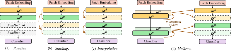
Figure 2: Variants of the growth operator $\bm{\zeta}$. $\bm{\omega}^{\textit{A}}$ and $\bm{\omega}^{\textit{B}}$ denote the parameters of two Transformer blocks in the original small network $\bm{\psi}_{s}$. (a) RandInit randomly initializes newly added layers; (b) Stacking duplicates the original layers and directly stacks the duplicated ones on top of them; (c) Interpolation interpolate new layers of $\bm{\psi}_{\ell}$ in between original ones and copy the weights from their nearest neighbor in $\bm{\psi}_{s}$. (d) Our proposed MoGrow is build upon Interpolation, by coping parameters $\widetilde{\bm{\omega}}$ from the momentum updated ensemble of $\bm{\psi}_{s}$.

In this section, we aim to develop a strong manual baseline for progressive learning of ViTs. We start by formulating progressive learning with its two main factors, growth schedule and growth operator in Sec. 3.1. Then, we present the growth space that we use in Sec. 3.2. Finally, we explore the most suitable growth operator of ViTs in Sec. 3.3.

Notations. We denote scalars, tensors and sets (or sequences) using lowercase, bold lowercase and uppercase letters (e.g., $n$, $\bm{x}$ and $\Psi$). For simplicity, we use $\{\bm{x}_{n}\}$ to denote the set $\{\bm{x}_{n}\}^{|n|}_{n=1}$ with cardinality $|n|$, similarly for a sequence $\left(\bm{x}_{n}\right)^{|n|}_{n=1}$. Please refer to Tab. 2 for a vis-to-vis explanation of the notations we used.

3.1 Progressive Learning

Progressive learning gradually increases the training overload by growing among its sub-networks following a growth schedule $\Psi$, which can be denoted by a sequence of sub-networks with increasing sizes for all the training epochs $t$. In practice, to ensure the network is sufficiently optimized after each growth, it is a common practice [82, 27, 69] to divide the whole training process into $|k|$ equispaced stages with $\tau=|t|/|k|$ epochs in each stage. Thus, the growth schedule can be denoted as ${\Psi=\Big{(}\bm{\psi}_{k}\Big{)}_{k=1}^{|k|}}$; the final one is always the complete model. Note that stages with different lengths can be achieved by using the same $\bm{\psi}$ in different numbers of consecutive stages, e.g., ${\Psi=(\bm{\psi}_{a},\bm{\psi}_{b},\bm{\psi}_{b})}$, where $\bm{\psi}_{a},\bm{\psi}_{b}$ are two different sub-networks.

When growing a sub-network to a larger one, the parameters of the larger sub-network are initialized by a growth operator $\bm{\zeta}$, which is a reparameterization function that maps the weights $\bm{\omega}_{s}$ of a smaller network to $\bm{\omega}_{\ell}$ of a larger one by ${\bm{\omega}_{\ell}=\bm{\zeta}(\bm{\omega}_{s})}$. The whole progress of progressive learning is summarized in Algorithm 1.

Notation	Type	Description
$t$, $|t|$	scalar	training epoch, total training epochs
$k$, $|k|$	scalar	training stage, total training stages
$\tau$	scalar	epochs per stage
$\Psi$	sequence	growth schedule
$\bm{\zeta}$	function	growth operator
$\bm{\psi}$	network	sub-network
$\Phi$	network	supernet
$\bm{\omega}$, $|\bm{\omega}|$	parameter	network parameters, number of parameters
$\Omega$, $\Lambda$	set	the whole growth space, partial growth space
$*$, $\star$	notation	optimal, relaxed optimal

Table 2: Notations describing progressive learning and automated progressive learning.

Input:

$\Psi$: the growth schedule; $\bm{\zeta}$: the growth operator;

$|t|$: total training epochs; $\tau$: epochs per stage;

Randomly initialized parameters $\bm{\omega}$;

for $t\in[1,|t|]$ do

       if   $t=N\tau,~{}~{}N\in\mathbb{N_{+}}$   then

             Switch to the sub-network of next stage  $\bm{\psi}\leftarrow\Psi[t/\tau]$;

             Initialize parameters by growth operator  $\bm{\omega}\leftarrow\bm{\zeta}(\bm{\omega})$;

       end if

       Train $\bm{\psi}(\bm{\omega})$ over all the training data.

end for

Algorithm 1 Progressive Learning

Let $\mathcal{L}$ be the target loss function, and $\mathcal{T}$ be the total runtime; then progressive learning can be formulated as:

$$\mathop{\min}_{\bm{\omega},\Psi,\bm{\zeta}}\big{\{}\mathcal{L}(\bm{\omega},\Psi,\bm{\zeta}),\mathcal{T}(\Psi)\big{\}},$$ (1)

where $\bm{\omega}$ denotes the parameters of sampled sub-networks during the optimization. Growth schedule $\Psi$ and growth operator $\bm{\zeta}$ have been explored for language Transformers [25, 27]. However, ViTs differ considerably from their linguistic counterparts. The huge difference on task objective, data distribution and network architecture could lead to drastic difference in optimal $\Psi$ and $\bm{\zeta}$. In the following parts of this section, we mainly study the growth operator $\bm{\zeta}$ for ViTs by fixing $\Psi$ as a uniform linear schedule in a growth space $\Omega$, and leave automatic exploration of $\Psi$ to Sec. 4.

3.2 Growth Space in Vision Transformers

The model capacity of ViTs are controlled by many factors, such as number of patches, network depth, embedding dimensions, MLP ratio, etc. In analogy to previous discoveries on fast compound model scaling [19], we empirically find that reducing network width (e.g., embedding dimensions) yields relatively smaller wall-time acceleration on modern GPUs when comparing at the same flops. Thus, we mainly study number of patchs ($n^{2}$) and network depth ($l$), leaving other dimensions for future works.

Number of Patches. Given patch size $p\times p$, input size ${r\times r}$, the number of patches $n\times n$ is determined by $n^{2}=r^{2}/p^{2}$. Thus, by fixing the patch size, reducing number of patches can be simply achieved by down-sampling the input image. However, in ViTs, the size of positional encoding is related to $n$. To overcome this limitation, we adaptively interpolate the positional encoding to match with $n$.

Network Depth. Network depth ($l$) is the number of Transformer blocks or its variants (e.g., Outlooker blocks [88]).

Uniform Linear Growth Schedule. To ablate the optimization of growth operator $\bm{\zeta}$, we fix growth schedule $\Psi$ as a uniform linear growth schedule. To be specific, “uniform” means that all the dimensions (i.e., $n$ and $l$) are scaled by the same ratio $s_{t}$ at the $t$-th epoch; “linear” means that the ratio $s$ grows linearly from $s_{1}$ to $1$. This manual schedule has only one hyper-parameter, the initial scaling ratio $s_{1}$, which is set to $0.5$ by default. With this fixed $\Psi$, the optimization of progressive learning in Eq. 1 is simplified to:

$$\mathop{\min}_{\bm{\omega},\bm{\zeta}}\mathcal{L}(\bm{\omega},\bm{\zeta}),$$ (2)

which enables direct optimization of $\bm{\zeta}$ by comparing the final accuracy after training with different $\bm{\zeta}$.

3.3 On the Growth of Vision Transformers

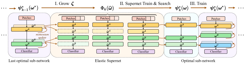
Figure 3: Pipeline of the $k$-th stage of automated progressive learning. In the beginning of the stage, the last optimal sub-network $\bm{\psi}^{\star}_{k-1}$ first grows to the Elastic Supernet $\Phi_{k}$ by $\widehat{\bm{\omega}}=\bm{\zeta}(\bm{\omega}^{\star})$; then, we search for the optimal sub-network $\bm{\psi}^{\star}_{k}$ after supernet training; finally, the sub-network is trained in the remaining epochs of this stage. The whole process of AutoProg is summarized in Algorithm 2.

Fig. 2 (a)-(c) depict the main variants of the growth operator $\bm{\zeta}$ that we compare, which cover choices from a wide range of the previous works, including RandInit [62], Stacking [25] and Interpolation [10, 20]. More formal definitions of these schemes can be found in the supplementary material. Our empirical comparison (in Sec. 5.3) shows Interpolation growth is the most suitable scheme for ViTs.

Unfortunately, growing by Interpolation changes the original function of the network. In practice, function perturbation brought by growth can result in significant performance drop, which is hardly recovered in subsequent training steps. Early works advocate for function-preserving growth operators [12, 78], which we denote by Identity. However, we empirically found growing by Identity greatly harms the performance on ViTs (see Sec. 5.3). Differently, we propose a growth operator, named Momentum Growth (MoGrow), to bridge the gap brought by model growth.

Momentum Growth (MoGrow). In recent years, a growing number of self-supervised [26, 28, 30] and semi-supervised [42, 71] methods learn knowledge from the historical ensemble of the network. Inspired by this, we propose to transfer knowledge from a momentum network during growth. This momentum network has the same architecture with $\bm{\psi}_{s}$ and its parameters $\bm{\widetilde{\omega}}_{s}$ are updated with the online parameters $\bm{\omega}_{s}$ in every training step by:

$$\bm{\widetilde{\omega}}_{s}\leftarrow m\bm{\widetilde{\omega}}_{s}+(1-m)\bm{\omega}_{s},$$ (3)

where $m$ is a momentum coefficient set to $0.998$. As the the momentum network usually has better generalization ability and better performance during training, loading parameters from the momentum network would help the model bypass the function perturbation gap. As shown in Fig. 2 (d), MoGrow is proposed upon Interpolation growth by maintaining a momentum network, and directly copying from it when performing network growth. MoGrow operator $\bm{\zeta}_{\textit{MoGrow}}$ can be simply defined as:

$$\bm{\zeta}_{\textit{MoGrow}}(\bm{\omega}_{s})=\bm{\zeta}_{\textit{Interpolation}}\big{(}\bm{\widetilde{\omega}}_{s}\big{)}.$$ (4)

4 Automated Progressive Learning

Input:

$\bm{\zeta}$: the growth operator;

$|t|$: total training epochs; $\tau$: epochs per stage;

Random initialize parameters $\bm{\omega}$;

for $t\in[1,|t|]$ do

       if   $t=N\tau,~{}~{}N\in\mathbb{N_{+}}$   then

             Switch optimizers to Elastic Supernet  $\Phi$;

             Initialize supernet parameters  $\widehat{\bm{\omega}}\leftarrow\bm{\zeta}(\bm{\omega})$;

       end if

       if   $t=N\tau+2,~{}~{}N\in\mathbb{N_{+}}$   then

             Search for the optimal sub-network $\bm{\psi}$ by Eq. 9;

             Switch to the optimal sub-network  $\bm{\psi}\leftarrow\bm{\psi}^{\star}$;

             Inherit parameters from the supernet  $\bm{\omega}\leftarrow\widehat{\bm{\omega}}$;

       end if

       Train $\bm{\psi}(\bm{\omega})$ or supernet $\Phi(\widehat{\bm{\omega}})$ over all the training data.

end for

Algorithm 2 Automated Progressive Learning

In this section, we focus on optimizing the growth schedule $\Psi$ by fixing the growth operator as $\bm{\zeta}_{\textit{MoGrow}}$. We first formulate the multi-objective optimization problem of $\Psi$, then propose our solution, called AutoProg, which is introduced in detail by its two estimation steps in Sec. 4.2 and Sec. 4.3.

4.1 Problem Formulation

The problem of designing growth schedule $\Psi$ for efficient training is a multi-objective optimization problem [16]. By fixing $\bm{\zeta}$ in Eq. 1 as our proposed $\bm{\zeta}_{\textit{MoGrow}}$, the objective of designing growth schedule $\Psi$ is:

$$\mathop{\min}_{\bm{\omega},\Psi}\big{\{}\mathcal{L}(\bm{\omega},\Psi),\mathcal{T}(\Psi)\big{\}}.$$ (5)

Note that multi-objective optimization problem has a set of Pareto optimal [16] solutions which can be approximated using customized weighted product, a common practice used in previous Auto-ML algorithms [67, 68]. In the scenario of progressive learning, the optimization objective can be defined as:

$$\mathop{\min}_{\bm{\omega},\Psi}\mathcal{L}(\bm{\omega},\Psi)\cdot\mathcal{T}(\Psi)^{\alpha},$$ (6)

where $\alpha$ is a balancing factor dynamically chosen by balancing the scores for all the candidate sub-networks.

4.2 Automated Progressive Learning by Optimizing Sub-Network Architectures

Denoting $|\bm{\psi}|$ the number of candidate sub-networks, and $|k|$ the number of stages, the number of candidate growth schedule is thus $|\bm{\psi}|^{|k|}$. As optimization of Eq. 6 contains optimization of network parameters $\bm{\omega}$, to get the final loss, a full $|t|$ epochs training with growth schedule $\Psi$ is required:

$$\Psi^{*}=\mathop{\arg\min}_{\Psi}\mathcal{L}\big{(}\bm{\omega}^{*}(\Psi);\bm{x}\big{)}\cdot\mathcal{T}(\Psi)^{\alpha}$$ (7)

$${\text{s.t.}}~{}~{}~{}~{}\bm{\omega}^{*}(\Psi)=\mathop{\arg\min}_{\bm{\omega}}\mathcal{L}(\Psi,{\bm{\omega}};\bm{x}).$$

Thus, performing an extensive search over the higher level factor $\Psi$ in this bi-level optimization problem has complexity $\mathcal{O}(|\bm{\psi}|^{|k|}\cdot|t|)$. Its expensive cost deviates from the original intention of efficient training.

To reduce the search cost, we relax the original objective of growth schedule search to progressively deciding whether, where and how much should the model grow, by searching the optimal sub-network architecture $\bm{\psi}^{*}_{k}$ in each stage $k$. Thus, the relaxed optimal growth schedule can be denoted as ${\Psi^{\star}=\Big{(}\bm{\psi}^{*}_{k}\Big{)}_{k=1}^{|k|}}$.

In sparse training and efficient Auto-ML algorithms, it is a common practice to estimate future ranking of models with current parameters and their gradients [22, 70], or with parameters after a single step of gradient descent update [55, 9, 53]. However, these methods are not suitable for progressive training, as the network function is drastically changed and is not stable after growth. We empirically found that the network parameters adapt quickly after growth and are already stable after one epoch of training. To make a good tradeoff between accuracy and training speed, we estimate the performance of each sub-network $\bm{\psi}$ in each stage by their training loss after the first two training epochs in this stage. Denoting $\bm{\omega}^{\star}$ the sub-network parameters obtained by two epochs of training, the optimal sub-network can be searched by:

$$\bm{\psi}_{k}^{*}=\mathop{\arg\min}_{\bm{\psi}_{k}\in\Lambda_{k}}\mathcal{L}\big{(}\bm{\omega}^{\star}(\bm{\psi}_{k});\bm{x}\big{)}\cdot\mathcal{T}(\bm{\psi}_{k})^{\alpha},$$ (8)

where $$\Lambda_{k}=\Big{\{}\bm{\psi}\in\Omega~{}\Big{|}~{}|\bm{\omega}(\bm{\psi})|\geq|\bm{\omega}(\bm{\psi}_{k})|\Big{\}},$$

where $\Lambda_{k}$ denotes the growth space of the $k$-th stage, containing all the sub-networks that are larger than or equal to the last optimal sub-network in terms of the number of parameters $|\bm{\omega}|$.

Overall, by relaxing the original optimization problem in Eq. 7 to Eq. 8, we only have to train each of the ${|\Lambda_{k}|}$ sub-networks for two epochs in each of the $|k|$ stages. Thus, the search complexity is reduced exponentially from $\mathcal{O}(|\bm{\psi}|^{|k|}\cdot|t|)$ to $\mathcal{O}(|\Lambda_{k}|\cdot|k|)$, where $|\Lambda_{k}|\leq|\bm{\psi}|$ and $|k|\leq|t|$.

4.3 One-shot Estimation of Sub-Network Performance via Elastic Supernet

Though we relax the optimization problem with significant search cost reduction, obtaining $\bm{\omega}^{\star}$ in Eq. 8 still takes ${2|\Lambda_{k}|}$ epochs for each stage, which will bring huge searching overhead to the progressive learning. The inefficiency of loss prediction is caused by the repeated training of sub-networks weight $\bm{\omega}$, with bi-level optimization being its nature. To circumvent this problem, we propose to share and jointly optimize sub-network parameters in $\Lambda_{k}$ via an Elastic Supernet with Interpolation.

Elastic Supernet with Interpolation. An Elastic Supernet $\Phi({\widehat{\bm{\omega}}})$ is a weight-nesting network parameterized by $\widehat{\bm{\omega}}$, and is able to execute with its sub-networks $\{\bm{\psi}\}$. Here, we give the formal definition of weight-nesting:

Definition 1

(weight-nesting) For any pair of sub-networks $\bm{\psi}_{a}(\bm{\omega}_{a})$ and $\bm{\psi}_{b}(\bm{\omega}_{b})$ in supernet $\Phi$, where $|\bm{\omega}_{a}|\leq|\bm{\omega}_{b}|$, if $\bm{\omega}_{a}\subseteq\bm{\omega}_{b}$ is always satisfied, then $\Phi$ is weight-nesting.

In previous works, a network with elastic depth is usually achieved by using the first layers to form sub-networks [36, 86, 11]. However, using this scheme after growing by Interpolation or MoGrow will cause inconsistency between expected sub-networks after growth and sub-networks in $\Phi$.

To solve this issue, we present an Elastic Supernet with Interpolation, with optionally activated layers interpolated in between always activated ones. As shown in Fig. 3, beginning from the smaller network in the last stage $\bm{\psi}^{\star}_{k-1}$, sub-networks in $\Phi$ are formed by inserting layers in between the original layers of $\bm{\psi}^{\star}_{k-1}$ (starting from the final layers), until reaching the largest sub-network in $\Lambda_{k}$.

Training and Searching via Elastic Supernet. By nesting parameters of all the candidate sub-networks in the Elastic supernet $\Phi$, the optimization of $\bm{\omega}$ is disentangled from $\bm{\psi}$. Thus, Eq. 8 is further relaxed to

$$\bm{\psi}_{k}^{\star}=\mathop{\arg\min}_{\bm{\psi}_{k}\in\Lambda_{k}}\mathcal{L}\big{(}\widehat{\bm{\omega}}^{\star};\bm{x}\big{)}\cdot\mathcal{T}(\bm{\psi}_{k})^{\alpha}$$ (9)

s.t. $$\widehat{\bm{\omega}}^{\star}=\mathop{\arg\min}^{~{}}_{\widehat{\bm{\omega}}}\mathbb{E}_{\bm{\psi}_{k}\in\Lambda_{k}}\big{\{}\mathcal{L}(\bm{\psi}_{k},\widehat{\bm{\omega}};\bm{x})\big{\}},$$

where the optimal nested parameters $\widehat{\bm{\omega}}^{\star}$ can be obtained by one-shot training of $\Phi$ for two epochs. For efficiency, we train $\Phi$ by randomly sampling only one of its sub-networks in each step (following [11]), instead of four in [85, 84, 86].

After training all the candidate sub-networks in the Elastic Supernet $\Phi$ concurrently for two epochs, we have the adapted supernet parameters $\widehat{\bm{\omega}}^{\star}$ that can be used to estimate the real performance of the sub-networks (i.e. performance when trained in isolation). As the sub-network grow space $\Lambda_{k}$ in each stage is relatively small, we can directly perform traversal search in $\Lambda_{k}$, by testing its training loss with a small subset of the training data. We use fixed data augmentation to ensure fair comparison, following [48]. Benefiting from parameter nesting and one-shot training of all the sub-networks in $\Lambda_{k}$, the search complexity is further reduced from $\mathcal{O}(|\Lambda_{k}|\cdot|k|)$ to $\mathcal{O}(|k|)$.

Weight Recycling. Benefiting from synergy of different sub-networks, the supernet converges at a comparable speed to training these sub-networks in isolation. Similar phenomenon can be observed in network regularization [64, 37], network augmentation [7], and previous elastic models [87, 86, 11]. Motivated by this, the searched sub-network directly inherits its parameters in the supernet to continue training. Benefiting from this weight recycling scheme, AutoProg has no extra searching epochs, since the supernet training epochs are parts of the whole training epochs. Moreover, as sampled sub-networks are faster than the full network, these supernet training epochs take less time than the original training epochs. Thus, the searching cost is directly reduced from $\mathcal{O}(|k|)$ to zero.

Model	Training scheme	Speedup runtime	Top-1 (%)	Top-1@288 (%)
100 epochs
DeiT-S [72]	Original	-	74.1	74.6
	Prog	+53.6%	72.6	73.2
	AutoProg	+40.7%	74.4	74.9
VOLO-D1 [88]	Original	-	82.6	83.0
	Prog	+60.9%	81.7	82.1
	AutoProg 0.5$\Omega$	+65.6%	82.8	83.2
	AutoProg 0.4$\Omega$	+85.1%	82.7	83.1
VOLO-D2 [88]	Original	-	83.6	84.1
	Prog	+54.4%	82.9	83.3
	AutoProg	+45.3%	83.8	84.2
300 epochs
DeiT-Tiny [72]	Original	-	72.2	72.9
	AutoProg	+51.2%	72.4	73.0
DeiT-S [72]	Original	-	79.8	80.1
	AutoProg	+42.0%	79.8	80.1
VOLO-D1 [88]	Original	-	84.2	84.4
	AutoProg	+48.9%	84.3	84.6
VOLO-D2 [88]	Original	-	85.2	85.1
	AutoProg	+42.7%	85.2	85.2

Table 3: Main results of efficient training on ImageNet. Accelerations that cause accuracy drop are marked with gray. Best results are marked with Bold; our method or default settings are highlighted in purple. Top-1@288 denotes Top-1 Accuracy when directly testing on 288$\times$288 input size, without finetuning. Please refer to the supplementary file for detailed FLOPs and runtime.

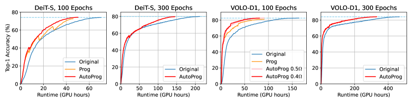
Figure 4: Evaluation accuracy of DeiT-S and VOLO-D1 during training with different learning schemes. Curves are not smoothed.

5 Experiments

Datasets. We evaluate our method on a large scale image classification dataset, ImageNet-1K [17] and two widely used classification datasets, CIFAR-10 and CIFAR-100 [41], for transfer learning. ImageNet contains 1.2M train set images and 50K val set images in 1,000 classes. We use all the training data for progressive learning and supernet training, and use a 50K randomly sampled subset to calculate training loss for sub-network search.

Architectures. We use two representative ViT architectures, DeiT [72] and VOLO [88] to evaluate the proposed AutoProg. Specifically, DeiT [72] is a representative standard ViT model; VOLO [88] is a hybrid architecture comprised of outlook attention blocks and transformer blocks.

Implementation Details. For both architectures, we use the original training hyper-parameters, data augmentation and regularization techniques of their corresponding prototypes [72, 88]. Our experiments are conducted on NVIDIA 3090 GPUs. As the acceleration achieved by our method is orthogonal to the acceleration of mixed precision training [58], we use it in both original baseline training and our progressive learning.

Grow Space $\bm{\Omega}$. We use 4 stages for progressive learning. The initial scaling ratio $s_{1}$ is set to ${0.5}$ or $0.4$; the corresponding grow spaces are denoted by $0.5\Omega$ and $0.4\Omega$. By default, we use $0.5\Omega$ for our experiments, unless mentioned otherwise. The grow space of $n$ and $l$ are calculated by multiplying the value of the whole model with 4 equispaced scaling ratios $s\in\{0.5,0.67,0.83,1.0\}$, and we round the results to valid integer values. We use Prog to denote our manual progressive baseline with uniform linear growth schedule as described in Sec. 3.2.

5.1 Efficient Training on ImageNet

We first validate the effectiveness of AutoProg on ImageNet. As shown in Tab. 3, AutoProg consistently achieves remarkable efficient training results on diverse ViT architectures and training schedules.

First, our AutoProg achieves significant training acceleration over the regular training scheme with no performance drop. Generally, AutoProg speeds up ViTs training by more than 45% despite changes on training epochs and network architectures. In particular, VOLO-D1 trained with AutoProg 0.4$\Omega$ achieves 85.1% training acceleration, and even slightly improves the accuracy (+0.1%). Second, AutoProg outperforms the manual baseline, the uniform linear growing (Prog), by a large margin. For instance, Prog scheme causes severe performance degradation on DeiT-S. AutoProg improves over Prog scheme on DeiT-S by 1.7% on accuracy, successfully eliminating the performance gap by automatically choosing the proper growth schedule. Third, as progressive learning uses smaller input size during training, one may question its generalization capability on larger input sizes. We answer this by directly testing the models trained with AutoProg on 288$\times$288 input size. The results justify that models trained with AutoProg have comparable generalization ability on larger input sizes to original models. Remarkably, VOLO-D1 trained for 300 epochs with AutoProg reaches 84.6% Top-1 accuracy when testing on 288$\times$288 input size, with 48.9% faster training.

The learning curves (i.e., evaluation accuracy during training) of DeiT-S and VOLO-D1 with different training schemes are shown in Fig. 4. Autoprog clearly accelerates the training progress of these two models. Interestingly, DeiT-S (100 epochs) trained with manual Prog scheme presents sharp fluctuations after growth, while AutoProg successfully addresses this issue and eventually reaches higher accuracy by choosing proper growth schedule.

5.2 Transfer Learning

Pretrain	Speedup	CIFAR-10	CIFAR-100
Original	-	99.0	89.5
AutoProg	48.9%	99.0	89.7

Table 4: Transfer learning results of DeiT-S on CIFAR datasets. The evaluation metric is Top-1 accuracy (%).

To further evaluate the transfer ability of ViTs trained with AutoProg, we conduct transfer learning on CIFAR-10 and CIFAR-100 datasets. We use the DeiT-S model that is pretrained with AutoProg on ImageNet for finetuning on CIFAR datasets, following the procedure in [72]. We compare with its counterpart pretrained with the ordinary training scheme. The results are summarized in Tab. 4. While AutoProg largely saves training time, it achieves competitive transfer learning results. This proves that AutoProg acceleration on ImageNet pretraining does not harm the transfer ability of ViTs on CIFAR datasets.

5.3 Ablation Study

Growth Operator $\bm{\zeta}$. We first compare the three growth operators mentioned in Sec. 3.3, i.e., RandInit [62], Stacking [25] and Interpolation [10, 20], by using them with manual Prog scheme on VOLO-D1. As shown in Tab. 5, Interpolation growth achieves the best accuracy both after the first growth and in the final.

Then, we compare two growth operators build upon Interpolation scheme, our proposed MoGrow, and Identity, which is a function-preserving [12, 78] operator that can be achieved by Interpolation + ReZero [1]. Specifically, ReZero uses a zero-initialized, learnable scalar to scale the residual modules in networks. Using this technique on newly added layers can assure the original network function is preserved. The results are shown in Tab. 5. Contrary to expectations, we observe that Identity growth largely reduces the Top-1 accuracy of VOLO-D1 (-3.21%), probably because the network convergence is slowed down by the small scalar; besides, the global minimum of the original function could be a local minimum in the new network, which hinders the optimization. On this inferior growth schedule, our MoGrow still improves over Interpolation by 0.15%, effectively reducing its performance gap.

Previous comparisons are based on the Prog scheme. Moreover, we also analyze the effect of MoGrow on AutoProg. The results are shown in Tab. 6. We observe that MoGrow largely improves the performance of the supernet by 2.73%. It also increases the final training accuracy by 0.2%, proving the effectiveness of MoGrow in AutoProg.

Growth Op. $\bm{\zeta}$	Top-1@Growth (%)	Top-1 (%)
Baseline	-	82.53
RandInit [62]	60.61	80.02
Stacking [25]	61.50	81.55
Interpolation [10, 20]	61.53	81.78
Identity [12, 78]	61.04	79.32
MoGrow	61.65	81.90

Table 5: Ablation analysis of depth growth operator $\bm{\zeta}$ with the Prog learning scheme. Top-1@Growth denotes the accuracy after training for the first epoch of the second stage.

Method	Top-1@Growth (%)	Top-1 (%)
AutoProg w/o MoGrow	59.41	82.6
AutoProg w/ MoGrow	62.14	82.8

Table 6: Ablation analysis of MoGrow in our AutoProg learning scheme on VOLO-D1. Top-1@Growth denotes the accuracy of the supernet after training for the first epoch of the second stage.

Weight Recycling. We further study the effect of weight recycling by training VOLO-D1 using AutoProg. As shown in Tab. 7, by recycling the weights of the supernet, AutoProg can achieve 12.3% more speedup. Also, benefiting from the synergy effect in weight-nesting [87], weight recycling scheme does not cause accuracy drop. These results prove the effectiveness of weight recycling.

Adaptive Regularization. Adaptive Regularization (AdaReg) for progressive learning is proposed in [69]. It adaptively change regularization intensity (including RandAug [14], Mixup [91] and Dropout [64]) according to network capacity of CNNs. Here, we generalize this scheme to ViTs and study its effect on ViT AutoProg training with DeiT-S and VOLO-D1. We mainly focus on three data augmentation and regularization techniques that are commonly used by ViTs, i.e., RandAug [14], stochastic depth [37] and random erase [93]. When using AdaReg scheme, we linearly increase the magnitude of RandAug from 0.5$\times$ to 1$\times$ of its original value, and also linearly increase the probabilities of stochastic depth and random erase from 0 to their original values. The results of AutoProg with and without AdaReg are shown in Tab. 8. Notably, DeiT-S can not converge when training with AdaReg, probably because DeiT models are heavily dependent on strong augmentations. On the contrary, AdaReg on VOLO-D1 is indispensable. Not using AdaReg causes 1.2% accuracy drop on VOLO-D1. This result is consistent with previous discoveries on CNNs [69]. By default, we use AdaReg on VOLO models and not use it on DeiT models.

Method	Speedup	Top-1 Acc. (%)
w/o recycling	53.3%	82.8
w/ recycling	65.6%	82.8

Table 7: Ablation analysis of weight recycling in our AutoProg learning scheme on VOLO-D1.

Method	AdaReg	Speedup	Top-1 Acc. (%)
DeiT-S AutoProg	✗	+40.7%	74.4
DeiT-S AutoProg	✓	-	00.1∗
VOLO-D1 AutoProg	✗	+50.9%	81.5
VOLO-D1 AutoProg	✓	+85.1%	82.7

Table 8: Ablation analysis of the adaptive regularization on ViTs with the AutoProg learning scheme. (*: training can not converge)

6 Conclusion and Discussion

In this paper, we take a practical step towards sustainable deep learning by generalizing and automating progressive learning for ViTs. We have developed a strong manual baseline for progressive learning of ViTs with MoGrow growth operator and proposed an automated progressive learning (AutoProg) scheme for automated growth schedule search. Our AutoProg has achieved consistent training speedup on different ViT models with lossless performance on ImageNet and transfer learning. Ablation studies have proved the effectiveness of each component of AutoProg.

Social Impact and Limitations. When network training becomes more efficient, it is also more available and less subject to regularization and study, which may result in a proliferation of models with harmful biases or intended uses. In this work, we achieve inspiring results with automated progressive learning on ViTs. However, large scale training of CNNs and language models can not directly benefit from it. We encourage future works to develop automated progressive learning for efficient training in broader applications.

Automated Progressive Learning for Efficient Training of Vision Transformers
Supplementary Material Changlin Li^1,2,3  Bohan Zhuang³Corresponding author.  Guangrun Wang⁴  Xiaodan Liang⁵  Xiaojun Chang²  Yi Yang^6
1Baidu Research  ²ReLER, AAII, University of Technology Sydney
³Monash University  ⁴University of Oxford  ⁵Sun Yat-sen University  ⁶Zhejiang University
changlinli.ai@gmail.com, bohan.zhuang@monash.edu, wanggrun@gmail.com,
xdliang328@gmail.com, xiaojun.chang@uts.edu.au, yangyics@zju.edu.cn

Appendix A Definition of Compared Growth Operators

Given a smaller network $\bm{\psi}_{s}$ and a larger network $\bm{\psi}_{\ell}$, a growth operator $\bm{\zeta}$ maps the parameters of the smaller one $\bm{\omega}_{s}$ to the parameters of the larger one $\bm{\omega}_{\ell}$ by: $\bm{\omega}_{\ell}=\bm{\zeta}(\bm{\omega}_{s})$. Let $\bm{\omega}_{\ell}^{i}$ denotes the parameters of the $i$-th layer in $\bm{\psi}_{\ell}$. We consider several $\bm{\zeta}$ in depth dimension that maps $\bm{\omega}_{s}$ to layer $i$ of $\bm{\psi}_{\ell}$ by: $\bm{\omega}_{\ell}^{i}=\bm{\zeta}(\bm{\omega}_{s},i)$.

RandInit. RandInit copies the original layers in $\bm{\psi}_{s}$ and random initialize the newly added layers:

$$\bm{\zeta}_{\textit{RandInit}}(\bm{\omega}_{s},i)=\left\{\begin{aligned} \bm{\omega}_{s}^{i},~{}~{}~{}~{}~{}~{}~{}~{}~{}~{}~{}&i\leq l_{s}\\ \textit{RandInit},~{}~{}&i>l_{s}.\\ \end{aligned}\right.$$ (10)

Stacking. Stacking duplicates the original layers and directly stacks the duplicated ones on top of them:

$$\bm{\zeta}_{\textit{Stacking}}(\bm{\omega}_{s},i)=\bm{\omega}_{s}^{i\bmod{l_{s}}}.$$ (11)

Interpolation. Interpolation interpolates new layers of $\bm{\psi}_{\ell}$ in between original ones and copy the weights from their nearest neighbor in $\bm{\psi}_{s}$:

$$\bm{\zeta}_{\textit{Interpolation}}(\bm{\omega}_{s},i)=\bm{\omega}_{s}^{\lfloor i/l_{s}\rfloor}.$$ (12)

Appendix B Implementation Details

Our ImageNet training settings follow closely to the original training settings of DeiT [72] and VOLO [88], respectively. We use the AdamW optimizer [57] with an initial learning rate of 1e-3, a total batch size of 1024 and a weight decay rate of 5e-2 for both architectures. The learning rate decays following a cosine schedule with 20 epochs warm-up for VOLO models and 5 epochs warm-up for DeiT models. For both architectures, we use exponential moving average with best momentum factor in $\{0.998,0.9986,0.999,0.9996\}$.

For DeiT training, we use RandAugment [14] with 9 magnitude and 0.5 magnitude std., mixup [91] with 0.8 probability, cutmix [89] with 1.0 probability, random erasing [93] with 0.25 probability, stochastic depth [37] with 0.1 probability and repeated augmentation [33].

For VOLO training, we use RandAugment [14], random erasing [93], stochastic depth [37], token labeling with MixToken [38], with magnitude of RandAugment, probability of random erasing and stochastic depth adjusted by Adaptive Regularization.

Adaptive Regularization. The detailed settings of Adaptive Regularization for VOLO progressive training is shown in Tab. I. These hyper-parameters are set heuristically regarding the model size. They perform fairly well in our experiments, but could still be sub-optimal.

Regularization	D0		D1
	min	max	min	max
RandAugment [14]	4.5	9	4.5	9
Random Erasing [93]	0	0.25	0.0625	0.25
Stoch. Depth [37]	0	0.1	0.1	0.2

Table I: Adaptive Regularization Settings (magnitude of RandAugment [14], probability of Random Erasing [93] and Stochastic Depth [37]) for progressive training of VOLO models.

Model	Training scheme	FLOPs (avg. per step)	Speedup	Runtime (GPU Hours)	Speedup	Top-1 (%)	Top-1@288 (%)
100 epochs
DeiT-S [72]	Original	4.6G	-	71	-	74.1	74.6
	Prog	2.4G	+91.6%	46	+53.6%	72.6	73.2
	AutoProg	2.8G	+62.0%	50	+40.7%	74.4	74.9
VOLO-D1 [88]	Original	6.8G	-	150	-	82.6	83.0
	Prog	3.7G	+84.7%	93	+60.9%	81.7	82.1
	AutoProg 0.5$\Omega$	3.3G	+104.2%	91	+65.6%	82.8	83.2
	AutoProg 0.4$\Omega$	2.9G	+132.2%	81	+85.1%	82.7	83.1
VOLO-D2 [88]	Original	14.1G	-	277	-	83.6	84.1
	Prog	7.5G	+87.7%	180	+54.4%	82.9	83.3
	AutoProg	8.3G	+68.7%	191	+45.3%	83.8	84.2
300 epochs
DeiT-Tiny [72]	Original	1.2G	-	144	-	72.2	72.9
	AutoProg	0.7G	+82.1%	95	+51.2%	72.4	73.0
DeiT-S [72]	Original	4.6G	-	213	-	79.8	80.1
	AutoProg	2.8G	+62.0%	150	+42.0%	79.8	80.1
VOLO-D1 [88]	Original	6.8G	-	487	-	84.2	84.4
	AutoProg	4.0G	+68.9%	327	+48.9%	84.3	84.6
VOLO-D2 [88]	Original	14.1G	-	863	-	85.2	85.1
	AutoProg	8.8G	+60.7%	605	+42.7%	85.2	85.2

Table II: Detailed results of efficient training on ImageNet. Best results are marked with Bold; our method or default settings are highlighted in purple. Top-1@288 denotes Top-1 Accuracy when directly testing on 288$\times$288 input size, without finetuning. Runtime is rounded to integer.

Growth Space $\bm{\Lambda}_{\bm{k}}$ in Each Stage. We find emprically that the elastic supernet converges faster when the number of sub-networks are smaller. Thus, restricting the growth space $\Lambda_{k}$ in each stage could help the convergence of the supernet. In practice, we make the restriction that $|\Lambda_{k}|\leq 9$. Specifically, in the first stage, we use the largest, the smallest and the medium candidates of $n$ and $l$ in $\Omega$ to construct $\Lambda_{1}$, which makes it possible to route to the whole network and perform regular training if the growing “ticket” (suitable sub-network) does not exist. In each of the following stages, we include the next 3 candidates of $l$ and the next 1 candidate of $n$, forming a growth space with $2\times 4=8$ candidates.

Appendix C Additional Results

Theoretical Speedup. In Tab. II, we calculate the average FLOPs per step of different learning schemes. AutoProg consistently achieves more than 60% speedup on theoretical computation. Remarkably, VOLO-D1 trained for 100 epochs with AutoProg 0.4$\Omega$ achieves 132.2% theoretical acceleration. The gap between theoretical and practical speedup indicates large potential of AutoProg. We leave the further improvement of practical speedup to future works; for example, AutoProg can be further accelerated by adjusting the batch size to fill up the GPU memory during progressive learning.

Comparison with Progressively Stacking. Progressively Stacking [25] (ProgStack) is a popular progressive learning method in NLP to accelerate BERT pretraining. It begins from $\frac{1}{4}$ of original layers, then copies and stacks the layers twice during training. Originally, it has three training stages with number of steps following a ratio 5:7:28. In CompoundGrow [27], this baseline is implemented as three stages with 3:4:3 step ratio. Our implementation follows closer to the original paper, using a ratio of 1:2:5. The results are shown in Tab. III. ProgStack achieves relatively small speedup with performance drop (0.4%). Our MoGrow reduces this performance gap to 0.1%. AutoProg achieves 74.1% more speedup and 0.5% accuracy improvement over the ProgStack baseline.

Training scheme	Runtime (GPU hours)	Speedup	Top-1 (%)
Baseline	150.2	-	82.6
ProgStack [25]	135.3	+11.0%	82.2
+ MoGrow	136.0	+10.4%	82.5
Prog	93.3	+60.9%	81.7
AutoProg 0.4$\Omega$	81.1	+85.1%	82.7

Table III: Comparison with progressively stacking.

Combine with AMP. Automatic mixed precision (AMP) [52] is a successful and mature low-bit precision efficient training method. We conduct experiments to prove that the speed-up achieved by AutoProg is orthogonal to that of AMP. As shown in Tab. IV, the relative speed-up achieved by AutoProg with or without AMP is comparable (+85.1% vs. +87.5%), proving the orthogonal speed-up.

Method	Speed-up	Top-1 Acc. (%)
Original (w/o AMP)	-	82.6
AMP	+74.0%	82.6
AutoProg	+87.5%	82.7
AMP + AutoProg	+222.1%	82.7
	(+85.1% over AMP)

Table IV: Speed-up of AutoProg is orthogonal to AMP [52].

Number of stages. We perform experiments to analyze the impact of the number of stages on AutoProg with different initial scaling ratios (0.5 and 0.4). As shown in Tab. V, AutoProg is not very sensitive to stage number settings. Fewer than 4 yields more speed-up, but could damage the performance. In general, the default 4 stages setting performs the best. When scaling the stage number to 50, there are only supernet training phases (2 epochs per stage) during the whole 100 epochs training, causing severe performance degradation.

Ratio	Num. Stages	Orig.	3	4	5	50
0.5	Speed-up	-	+69.1%	+65.6%	+63.6%	+48.5%
	Top-1 Acc. (%)	82.6	82.6	82.8	82.8	81.7
0.4	Speed-up	-	+90.8%	+85.1%	+80.4%	-
	Top-1 Acc. (%)	82.6	82.4	82.7	82.7	-

Table V: Ablation analysis on number of stages.

Effect of Progressive Learning in AutoProg. AutoProg is comprised by its two main components, “Auto” and “Prog”. The effectiveness of “Auto” is already studied by comparing with Prog in the main text. Here, we study the effectiveness of progressive learning in AutoProg by training an elastic supernet baseline for 100 epochs without progressive growing to compare with AutoProg. Specifically, we treat VOLO-D1 as an Elastic Supernet, and train it by randomly sampling one of its sub-networks in each step, same to the search stage in AutoProg. The results are shown in Tab. VI. In previous works that uses elastic supernet [87, 86, 11], the supernet usually requires more training iterations to reach a comparable performance to a single model. As expected, the supernet performance is lower than the original network given the same training epochs. Specifically, AutoProg improves over elastic supernet baseline by 1.1% Top-1 accuracy, with 17.1% higher training speedup, reaching the performance of the original model with the same training epochs but much faster, which proves the superiority of progressive learning.

Method	Speedup	Top-1 Acc. (%)
Original	-	82.6
Supernet	48.5%	81.7
AutoProg	65.6%	82.8

Table VI: Ablation analysis of progressive learning in AutoProg with VOLO-D1.

Analyse of Searched Growth Schedule. Two typical growth schedules searched by AutoProg are shown in Tab. VII. AutoProg clearly prefers smaller token number than smaller layer number. Nevertheless, selecting a small layer number in the first stage is still a good choice, as both of the two schemes use reduced layers in the first stage.

Stage $k$		1	2	3	4
VOLO-D1 100e 0.4$\Omega$	$l$	0.4	1	1	1
	$n$	0.4	0.6	0.6	1
VOLO-D2 300e	$l$	0.83	1	1	1
	$n$	0.5	0.67	0.83	1

Table VII: Searched growth schedules for VOLO-D1 0.4$\Omega$, 100 epochs, and VOLO-D2, 300 epochs.

Retraining with Searched Growth Schedule. To evaluate the searched growth schedule, we perform retraining from scratch with VOLO-D1, using the schedule searched by AutoProg 0.4$\Omega$. As shown in Tab. VIII, retraining takes slightly longer time (-0.6% speedup) because the speed of searched optimal sub-networks could be slightly slower than the average speed of sub-networks in the elastic supernet. Retraining reaches the same final accuracy, proving that the searched growth schedule can be used separately.

Training scheme	Runtime (GPU hours)	Speedup	Top-1 (%)
Baseline	150.2	-	82.6
AutoProg 0.4$\Omega$	81.1	+85.1%	82.7
Retrain	81.4	+84.5%	82.7

Table VIII: Retraining results with searched growth schedule on VOLO-D1, 100 epochs.

Extend to CNNs. To explore the effect of our policy on CNNs, we conduct experiments with ResNet50 [31], and found that the policy searched on ViTs generalizes very well on CNNs (see Tab. IX). These results imply that AutoProg opens an interesting direction (automated progressive learning) to develop more general learning methods for a wide computer vision field.

Method	Speed-up	Top-1 Acc. (%)
Original	-	77.3
AutoProg	+56.9%	77.3

Table IX: AutoProg with ResNet50 [31] on ImageNet (100 epochs).

References

- [1] Thomas C. Bachlechner, Bodhisattwa Prasad Majumder, Huanru Henry Mao, G. Cottrell, and Julian McAuley. Rezero is all you need: Fast convergence at large depth. arXiv preprint arXiv:2003.04887, 2020.
- [2] Bowen Baker, Otkrist Gupta, Nikhil Naik, and Ramesh Raskar. Designing neural network architectures using reinforcement learning. In ICLR, 2017.
- [3] Yoshua Bengio, Pascal Lamblin, Dan Popovici, and H. Larochelle. Greedy layer-wise training of deep networks. In NeurIPS, 2006.
- [4] James Bergstra, Rémi Bardenet, Yoshua Bengio, and Balázs Kégl. Algorithms for hyper-parameter optimization. In NeurIPS, 2011.
- [5] James Bergstra and Yoshua Bengio. Random search for hyper-parameter optimization. JMLR, 13, 2012.
- [6] Andrew Brock, Theodore Lim, James M. Ritchie, and Nick Weston. SMASH: one-shot model architecture search through hypernetworks. In ICLR, 2018.
- [7] Han Cai, Chuang Gan, Ji Lin, and Song Han. Network augmentation for tiny deep learning. arXiv preprint arXiv:2110.08890, 2021.
- [8] Han Cai, Chuang Gan, Tianzhe Wang, Zhekai Zhang, and Song Han. Once-for-all: Train one network and specialize it for efficient deployment. In ICLR, 2020.
- [9] Han Cai, Ligeng Zhu, and Song Han. Proxylessnas: Direct neural architecture search on target task and hardware. In ICLR, 2019.
- [10] Bo Chang, Lili Meng, Eldad Haber, Frederick Tung, and David Begert. Multi-level residual networks from dynamical systems view. In ICLR, 2018.
- [11] Minghao Chen, Houwen Peng, Jianlong Fu, and Haibin Ling. Autoformer: Searching transformers for visual recognition. In ICCV, 2021.
- [12] Tianqi Chen, Ian Goodfellow, and Jonathon Shlens. Net2net: Accelerating learning via knowledge transfer. In ICLR, 2016.
- [13] Ekin Dogus Cubuk, Barret Zoph, Dandelion Mané, Vijay Vasudevan, and Quoc V. Le. Autoaugment: Learning augmentation strategies from data. In CVPR, 2019.
- [14] Ekin Dogus Cubuk, Barret Zoph, Jonathon Shlens, and Quoc V. Le. Randaugment: Practical automated data augmentation with a reduced search space. In CVPRW, 2020.
- [15] Zihang Dai, Hanxiao Liu, Quoc V Le, and Mingxing Tan. Coatnet: Marrying convolution and attention for all data sizes. In NeurIPS, 2021.
- [16] Kalyanmoy Deb. Multi-objective optimization. In Search methodologies. Springer, 2014.
- [17] Jia Deng, Wei Dong, Richard Socher, Li-Jia Li, Kai Li, and Li Fei-Fei. Imagenet: A large-scale hierarchical image database. In CVPR, 2009.
- [18] Jacob Devlin, Ming-Wei Chang, Kenton Lee, and Kristina Toutanova. Bert: Pre-training of deep bidirectional transformers for language understanding. In NAACL, 2019.
- [19] Piotr Dollár, Mannat Singh, and Ross B. Girshick. Fast and accurate model scaling. In CVPR, 2021.
- [20] Chengyu Dong, Liyuan Liu, Zichao Li, and Jingbo Shang. Towards adaptive residual network training: A neural-ode perspective. In ICML, 2020.
- [21] Alexey Dosovitskiy, Lucas Beyer, Alexander Kolesnikov, Dirk Weissenborn, Xiaohua Zhai, Thomas Unterthiner, Mostafa Dehghani, Matthias Minderer, Georg Heigold, Sylvain Gelly, Jakob Uszkoreit, and Neil Houlsby. An image is worth 16x16 words: Transformers for image recognition at scale. In ICLR, 2021.
- [22] Utku Evci, Trevor Gale, Jacob Menick, Pablo Samuel Castro, and Erich Elsen. Rigging the lottery: Making all tickets winners. In ICML, 2020.
- [23] Scott E. Fahlman and Christian Lebiere. The cascade-correlation learning architecture. In NeurIPS, 1989.
- [24] Jonathan Frankle and Michael Carbin. The lottery ticket hypothesis: Finding sparse, trainable neural networks. In ICLR, 2019.
- [25] Linyuan Gong, Di He, Zhuohan Li, Tao Qin, Liwei Wang, and Tie-Yan Liu. Efficient training of bert by progressively stacking. In ICML, 2019.
- [26] Jean-Bastien Grill, Florian Strub, Florent Altché, Corentin Tallec, Pierre H. Richemond, Elena Buchatskaya, Carl Doersch, Bernardo Avila Pires, Zhaohan Daniel Guo, Mohammad Gheshlaghi Azar, Bilal Piot, Koray Kavukcuoglu, Rémi Munos, and Michal Valko. Bootstrap your own latent: A new approach to self-supervised learning. In NeurIPS, 2020.
- [27] Xiaotao Gu, Liyuan Liu, Hongkun Yu, Jing Li, Chen Chen, and Jiawei Han. On the transformer growth for progressive bert training. In NAACL, 2021.
- [28] Daniel Guo, Bernardo Avila Pires, Bilal Piot, Jean-bastien Grill, Florent Altché, Rémi Munos, and Mohammad Gheshlaghi Azar. Bootstrap latent-predictive representations for multitask reinforcement learning. In ICML, 2020.
- [29] Zichao Guo, Xiangyu Zhang, Haoyuan Mu, Wen Heng, Zechun Liu, Yichen Wei, and Jian Sun. Single path one-shot neural architecture search with uniform sampling. In ECCV, 2020.
- [30] Kaiming He, Haoqi Fan, Yuxin Wu, Saining Xie, and Ross B. Girshick. Momentum contrast for unsupervised visual representation learning. In CVPR, 2020.
- [31] Kaiming He, Xiangyu Zhang, Shaoqing Ren, and Jian Sun. Deep residual learning for image recognition. In CVPR, 2016.
- [32] Geoffrey E. Hinton, Simon Osindero, and Yee Whye Teh. A fast learning algorithm for deep belief nets. Neural Computation, 18, 2006.
- [33] Elad Hoffer, Tal Ben-Nun, Itay Hubara, Niv Giladi, Torsten Hoefler, and Daniel Soudry. Augment your batch: Improving generalization through instance repetition. In CVPR, 2020.
- [34] Lu Hou, Lifeng Shang, Xin Jiang, and Qun Liu. Dynabert: Dynamic bert with adaptive width and depth. In NeurIPS, 2020.
- [35] Hanzhang Hu, Debadeepta Dey, Martial Hebert, and J Andrew Bagnell. Learning anytime predictions in neural networks via adaptive loss balancing. In AAAI, 2019.
- [36] Gao Huang, Danlu Chen, Tianhong Li, Felix Wu, Laurens van der Maaten, and Kilian Q. Weinberger. Multi-scale dense networks for resource efficient image classification. In ICLR, 2018.
- [37] Gao Huang, Yu Sun, Zhuang Liu, Daniel Sedra, and Kilian Q. Weinberger. Deep networks with stochastic depth. In ECCV, 2016.
- [38] Zihang Jiang, Qibin Hou, Li Yuan, Daquan Zhou, Yujun Shi, Xiaojie Jin, Anran Wang, and Jiashi Feng. All tokens matter: Token labeling for training better vision transformers. arXiv preprint arXiv:2104.10858, 2021.
- [39] Tero Karras, Timo Aila, Samuli Laine, and Jaakko Lehtinen. Progressive growing of gans for improved quality, stability, and variation. In ICLR, 2018.
- [40] Hyunjik Kim, George Papamakarios, and Andriy Mnih. The lipschitz constant of self-attention. In ICML, 2021.
- [41] A. Krizhevsky and G. Hinton. Learning multiple layers of features from tiny images. Master’s thesis, Department of Computer Science, University of Toronto, 2009.
- [42] Samuli Laine and Timo Aila. Temporal ensembling for semi-supervised learning. arXiv preprint arXiv:1610.02242, 2016.
- [43] Gustav Larsson, Michael Maire, and Gregory Shakhnarovich. Fractalnet: Ultra-deep neural networks without residuals. In ICLR, 2017.
- [44] Hankook Lee and Jinwoo Shin. Anytime neural prediction via slicing networks vertically. arXiv preprint arXiv:1807.02609, 2018.
- [45] Régis Lengellé and Thierry Denoeux. Training mlps layer by layer using an objective function for internal representations. Neural Networks, 9, 1996.
- [46] Bei Li, Ziyang Wang, Hui Liu, Yufan Jiang, Quan Du, Tong Xiao, Huizhen Wang, and Jingbo Zhu. Shallow-to-deep training for neural machine translation. In EMNLP, 2020.
- [47] Changlin Li, Jiefeng Peng, Liuchun Yuan, Guangrun Wang, Xiaodan Liang, Liang Lin, and Xiaojun Chang. Block-wisely supervised neural architecture search with knowledge distillation. In CVPR, 2020.
- [48] Changlin Li, Tao Tang, Guangrun Wang, Jiefeng Peng, Bing Wang, Xiaodan Liang, and Xiaojun Chang. Bossnas: Exploring hybrid cnn-transformers with block-wisely self-supervised neural architecture search. In ICCV, 2021.
- [49] Changlin Li, Guangrun Wang, Bing Wang, Xiaodan Liang, Zhihui Li, and Xiaojun Chang. Ds-net++: Dynamic weight slicing for efficient inference in cnns and transformers. arXiv preprint arXiv:2109.10060, 2021.
- [50] Changlin Li, Guangrun Wang, Bing Wang, Xiaodan Liang, Zhihui Li, and Xiaojun Chang. Dynamic slimmable network. In CVPR, 2021.
- [51] Hao Li, Chenxin Tao, Xizhou Zhu, Xiaogang Wang, Gao Huang, and Jifeng Dai. Auto seg-loss: Searching metric surrogates for semantic segmentation. In ICLR, 2021.
- [52] Hao Li, Hong Zhang, Xiaojuan Qi, Ruigang Yang, and Gao Huang. Improved techniques for training adaptive deep networks. In ICCV, 2019.
- [53] Yonggang Li, Guosheng Hu, Yongtao Wang, Timothy M. Hospedales, Neil Martin Robertson, and Yongxing Yang. Dada: Differentiable automatic data augmentation. In ECCV, 2020.
- [54] Chenxi Liu, Barret Zoph, Maxim Neumann, Jonathon Shlens, Wei Hua, Li-Jia Li, Li Fei-Fei, Alan Yuille, Jonathan Huang, and Kevin Murphy. Progressive neural architecture search. In ECCV, 2018.
- [55] Hanxiao Liu, Karen Simonyan, and Yiming Yang. DARTS: differentiable architecture search. In ICLR, 2019.
- [56] Ze Liu, Yutong Lin, Yue Cao, Han Hu, Yixuan Wei, Zheng Zhang, Stephen Lin, and Baining Guo. Swin transformer: Hierarchical vision transformer using shifted windows. In ICCV, 2021.
- [57] Ilya Loshchilov and Frank Hutter. Decoupled weight decay regularization. In ICLR, 2019.
- [58] Paulius Micikevicius, Sharan Narang, Jonah Alben, Gregory Diamos, Erich Elsen, David Garcia, Boris Ginsburg, Michael Houston, Oleksii Kuchaiev, Ganesh Venkatesh, et al. Mixed precision training. In ICLR, 2018.
- [59] David Patterson, Joseph Gonzalez, Quoc V. Le, Chen Liang, Lluís-Miquel Munguía, Daniel Rothchild, David R. So, Maud Texier, and Jeff Dean. Carbon emissions and large neural network training. arXiv preprint arXiv:2104.10350, 2021.
- [60] Jiefeng Peng, Jiqi Zhang, Changlin Li, Guangrun Wang, Xiaodan Liang, and Liang Lin. Pi-nas: Improving neural architecture search by reducing supernet training consistency shift. In ICCV, 2021.
- [61] Hieu Pham, Melody Guan, Barret Zoph, Quoc Le, and Jeff Dean. Efficient neural architecture search via parameters sharing. In ICML, 2018.
- [62] Karen Simonyan and Andrew Zisserman. Very deep convolutional networks for large-scale image recognition. In ICLR, 2014.
- [63] Leslie N. Smith, Emily M. Hand, and Timothy Doster. Gradual dropin of layers to train very deep neural networks. In CVPR, 2016.
- [64] Nitish Srivastava, Geoffrey E. Hinton, Alex Krizhevsky, Ilya Sutskever, and Ruslan Salakhutdinov. Dropout: a simple way to prevent neural networks from overfitting. J. Mach. Learn. Res., 15, 2014.
- [65] Emma Strubell, Ananya Ganesh, and Andrew McCallum. Energy and policy considerations for deep learning in nlp. In ACL, 2019.
- [66] Chen Sun, Abhinav Shrivastava, Saurabh Singh, and Abhinav Gupta. Revisiting unreasonable effectiveness of data in deep learning era. In ICCV, 2017.
- [67] Mingxing Tan, Bo Chen, Ruoming Pang, Vijay Vasudevan, Mark Sandler, Andrew Howard, and Quoc V. Le. Mnasnet: Platform-aware neural architecture search for mobile. In CVPR, 2019.
- [68] Mingxing Tan and Quoc V. Le. Efficientnet: Rethinking model scaling for convolutional neural networks. In ICML, 2019.
- [69] Mingxing Tan and Quoc V. Le. Efficientnetv2: Smaller models and faster training. In ICML, 2021.
- [70] Hidenori Tanaka, Daniel Kunin, Daniel L Yamins, and Surya Ganguli. Pruning neural networks without any data by iteratively conserving synaptic flow. In NeurIPS, volume 33, 2020.
- [71] Antti Tarvainen and Harri Valpola. Mean teachers are better role models: Weight-averaged consistency targets improve semi-supervised deep learning results. In NeurIPS, 2017.
- [72] Hugo Touvron, Matthieu Cord, Matthijs Douze, Francisco Massa, Alexandre Sablayrolles, and Hervé Jégou. Training data-efficient image transformers & distillation through attention. In ICML, 2021.
- [73] Guangcong Wang, Xiaohua Xie, Jianhuang Lai, and Jiaxuan Zhuo. Deep growing learning. In ICCV, pages 2812–2820, 2017.
- [74] Jiachun Wang, Fajie Yuan, Jian Chen, Qingyao Wu, Min Yang, Yang Sun, and Guoxiao Zhang. Stackrec: Efficient training of very deep sequential recommender models by iterative stacking. In ACM SIGIR, 2021.
- [75] Yulin Wang, Rui Huang, Shiji Song, Zeyi Huang, and Gao Huang. Not all images are worth 16x16 words: Dynamic vision transformers with adaptive sequence length. In NeurIPS, 2021.
- [76] Tao Wei, Changhu Wang, and Chang Wen Chen. Modularized morphing of neural networks. arXiv preprint arXiv:1701.03281, 2017.
- [77] Tao Wei, Changhu Wang, and Chang Wen Chen. Modularized morphing of deep convolutional neural networks: A graph approach. IEEE Transactions on Computers, 70, 2021.
- [78] Tao Wei, Changhu Wang, Yong Rui, and Chang Wen Chen. Network morphism. In ICML, 2016.
- [79] Wei Wen, Feng Yan, and Hai Helen Li. Autogrow: Automatic layer growing in deep convolutional networks. In KDD, 2020.
- [80] Lijun Wu, Fei Tian, Yingce Xia, Yang Fan, Tao Qin, Jianhuang Lai, and Tie-Yan Liu. Learning to teach with dynamic loss functions. In NeurIPS, 2018.
- [81] Haowen Xu, H. Zhang, Zhiting Hu, Xiaodan Liang, Ruslan Salakhutdinov, and Eric P. Xing. Autoloss: Learning discrete schedules for alternate optimization. In ICLR, 2019.
- [82] Cheng Yang, Shengnan Wang, Chao Yang, Yuechuan Li, Ru He, and Jingqiao Zhang. Progressively stacking 2.0: A multi-stage layerwise training method for bert training speedup. arXiv preprint arXiv:2011.13635, 2020.
- [83] Yuning You, Tianlong Chen, Zhangyang Wang, and Yang Shen. L2-gcn: Layer-wise and learned efficient training of graph convolutional networks. In CVPR, 2020.
- [84] Jiahui Yu and Thomas Huang. Autoslim: Towards one-shot architecture search for channel numbers. In NeurIPS workshop, 2019.
- [85] Jiahui Yu and Thomas S. Huang. Universally slimmable networks and improved training techniques. In ICCV, 2019.
- [86] Jiahui Yu, Pengchong Jin, Hanxiao Liu, Gabriel Bender, Pieter-Jan Kindermans, Mingxing Tan, T. Huang, Xiaodan Song, and Quoc V. Le. Bignas: Scaling up neural architecture search with big single-stage models. In ECCV, 2020.
- [87] Jiahui Yu, Linjie Yang, Ning Xu, Jianchao Yang, and Thomas Huang. Slimmable neural networks. In ICLR, 2019.
- [88] Li Yuan, Qibin Hou, Zihang Jiang, Jiashi Feng, and Shuicheng Yan. VOLO: Vision outlooker for visual recognition. arXiv preprint arXiv:2106.13112, 2021.
- [89] Sangdoo Yun, Dongyoon Han, Seong Joon Oh, Sanghyuk Chun, Junsuk Choe, and Young Joon Yoo. Cutmix: Regularization strategy to train strong classifiers with localizable features. In ICCV, 2019.
- [90] Xiaohua Zhai, Alexander Kolesnikov, Neil Houlsby, and Lucas Beyer. Scaling vision transformers. arXiv preprint arXiv:2106.04560, 2021.
- [91] Hongyi Zhang, Moustapha Cissé, Yann Dauphin, and David Lopez-Paz. mixup: Beyond empirical risk minimization. In ICLR, 2018.
- [92] Minjia Zhang and Yuxiong He. Accelerating training of transformer-based language models with progressive layer dropping. In NeurIPS, 2020.
- [93] Zhun Zhong, Liang Zheng, Guoliang Kang, Shaozi Li, and Yi Yang. Random erasing data augmentation. In AAAI, 2020.
- [94] Barret Zoph and Quoc V. Le. Neural architecture search with reinforcement learning. In ICLR, 2017.