Catching Both Gray and Black Swans: Open-set Supervised Anomaly Detection

Abstract

Despite most existing anomaly detection studies assume the availability of normal training samples only, a few labeled anomaly examples are often available in many real-world applications, such as defect samples identified during random quality inspection, lesion images confirmed by radiologists in daily medical screening, etc. These anomaly examples provide valuable knowledge about the application-specific abnormality, enabling significantly improved detection of similar anomalies in some recent models. However, those anomalies seen during training often do not illustrate every possible class of anomaly, rendering these models ineffective in generalizing to unseen anomaly classes. This paper tackles open-set supervised anomaly detection, in which we learn detection models using the anomaly examples with the objective to detect both seen anomalies (‘gray swans’) and unseen anomalies (‘black swans’). We propose a novel approach that learns disentangled representations of abnormalities illustrated by seen anomalies, pseudo anomalies, and latent residual anomalies (i.e., samples that have unusual residuals compared to the normal data in a latent space), with the last two abnormalities designed to detect unseen anomalies. Extensive experiments on nine real-world anomaly detection datasets show superior performance of our model in detecting seen and unseen anomalies under diverse settings. Code and data are available at: https://github.com/choubo/DRA

1 Introduction

Anomaly detection (AD) aims at identifying exceptional samples that do not conform to expected patterns [36]. It has broad applications in diverse domains, e.g., lesion detection in medical image analysis [49, 71, 57], inspecting micro-cracks/defects in industrial inspection [3, 4], crime/accident detection in video surveillance [21, 52, 11, 70], and unknown object detection in autonomous driving [10, 56]. Most of existing anomaly detection methods [59, 47, 11, 60, 42, 2, 33, 39, 58, 74, 13, 39, 49, 46, 69, 44, 8] are unsupervised, which assume the availability of normal training samples only, i.e., anomaly-free training data, because it is difficult, if not impossible, to collect large-scale anomaly data. However, a small number of (e.g., one to multiple) labeled anomaly examples are often available in many relevant real-world applications, such as some defect samples identified during random quality inspection, lesion images confirmed by radiologists in daily medical screening, etc. These anomaly examples provide valuable knowledge about application-specific abnormality [45, 30, 37, 35], but the unsupervised detectors are unable to utilize them. Due to the lack of knowledge about anomalies, the learned features in unsupervised models are not discriminative enough to distinguish anomalies (especially some challenging ones) from normal data, as illustrated by the results of KDAD [47], a recent state-of-the-art (SotA) unsupervised method, on two MVTec AD defect detection datasets [3] in Fig. 1.

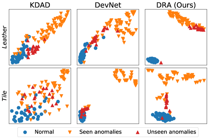
Figure 1: t-SNE visualization of features learned by SotA unsupervised (KDAD [47]) and supervised (DevNet [37, 35]) models, and our open-set supervised model (DRA) on the test data of two MVTec AD datasets, Leather and Tile. KDAD is trained with normal data only, learning less discriminative features than DevNet and DRA that are trained using ten samples from the seen anomaly classes, in addition to the normal data. DevNet is prone to overfitting the seen anomalies, failing to distinguish unseen anomalies from the normal data, while DRA effectively mitigates this issue.

In recent years, there have been some studies [45, 37, 35, 30] exploring a supervised detection paradigm that aims at exploiting those small, readily accessible anomaly data—rare but previously occurred exceptional cases/events, a.k.a. gray swans [23] – to train anomaly-informed detection models. The current methods in this line focus on fitting these anomaly examples using one-class metric learning with the anomalies as negative samples [45, 30] or one-sided anomaly-focused deviation loss [37, 35]. Despite the limited amount of the anomaly data, they achieve largely improved performance in detecting anomalies that are similar to the anomaly examples seen during training. However, these seen anomalies often do not illustrate every possible class of anomaly because i) anomalies per se are unknown and ii) the seen and unseen anomaly classes can differ largely from each other [36], e.g., the defective features of color stains are very different from that of folds and cuts in leather defect inspection. Consequently, these models can overfit the seen anomalies, failing to generalize to unseen/unknown anomaly classes—rare and previously unknown exceptional cases/events, a.k.a.  black swans [55], as shown by the result of DevNet [37, 35] in Fig. 1 where DevNet improves over KDAD in detecting the seen anomalies but fails to discriminate unseen anomalies from normal samples. In fact, these supervised models can be biased by the given anomaly examples and become less effective in detecting unseen anomalies than unsupervised detectors (see DevNet vs.  KDAD on the Tile dataset in Fig. 1).

To address this issue, this paper tackles open-set supervised anomaly detection, in which detection models are trained using the small anomaly examples in an open-set environment, i.e., the objective is to detect both seen anomalies (‘gray swans’) and unseen anomalies (‘black swans’). To this end, we propose a novel anomaly detection approach, termed DRA, that learns disentangled representations of abnormalities to enable the generalized detection. Particularly, we disentangle the unbounded abnormalities into three general categories: anomalies similar to the limited seen anomalies, anomalies that are similar to pseudo anomalies created from data augmentation or external data sources, and unseen anomalies that are detectable in some latent residual-based composite feature spaces. We further devise a multi-head network, with separate heads enforced to learn each type of these three disentangled abnormalities. In doing so, our model learns diversified abnormality representations rather than only the known abnormality, which can discriminate both seen and unseen anomalies from the normal data, as shown in Fig. 1.

In summary, we make the following main contributions:

• To tackle open-set supervised AD, we propose to learn disentangled representations of abnormalities illustrated by seen anomalies, pseudo anomalies, and latent residual-based anomalies. This learns diversified abnormality representations, extending the set of anomalies sought to both seen and unseen anomalies.

• We propose a novel multi-head neural network-based model DRA to learn the disentangled abnormality representations, with each head dedicated to capturing one specific type of abnormality.

• We further introduce a latent residual-based abnormality learning module that learns abnormality upon the residuals between the intermediate feature maps of normal and abnormal samples. This helps learn discriminative composite features for the detection of hard anomalies (e.g., unseen anomalies) that cannot be detected in the original non-composite feature space.

• We perform comprehensive experiments on nine real-application datasets from industrial inspection, rover-based planetary exploration and medical image analysis. The results show that our model substantially outperforms five SotA competing models in diverse settings. The results also establish new baselines for future work in this important emerging direction.

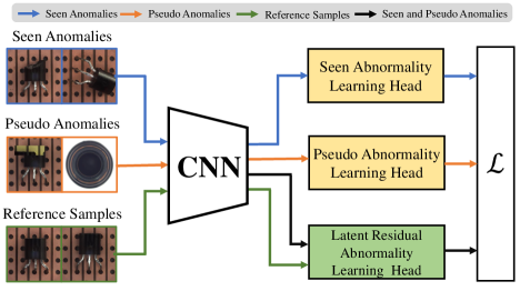
(a)

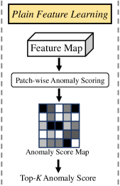
(b)

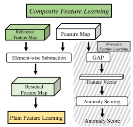
(c)

Figure 2: Overview of our proposed framework. (a) presents the high-level procedure of learning three disentangled abnormalities, (b) shows the abnormality feature learning in the plain (non-composite) feature space for the seen and pseudo abnormality learning heads, and (c) shows the framework of our proposed latent residual abnormality learning in a composite feature space.

2 Related Work

Unsupervised Approaches. Most existing anomaly detection methods, such as autoencoder-base methods [72, 13, 19, 39, 74], GAN-base methods [49, 40, 46, 69], self-supervised methods [12, 61, 2, 11, 51, 26, 57], and one-class classification methods [41, 44, 7, 8], assume that only normal data can be accessed during training. Although they do not have the risk of biasing towards the seen anomalies, they are difficult to distinguish anomalies from normal samples due to the lack of knowledge about true anomalies.

Supervised Approaches. A recently emerging direction focuses on supervised (or semi-supervised) anomaly detection that alleviates the lack of anomaly information by leveraging small anomaly examples to learn anomaly-informed models. This is achieved by one-class metric learning with the anomalies as negative samples [34, 45, 30, 14] or one-sided anomaly-focused deviation loss [37, 35, 71]. However, these models rely heavily on the seen anomalies and can overfit the known abnormality. A reinforcement learning approach is introduced in [38] to mitigate this overfitting issue, but it assumes the availability of large-scale unlabeled data and the presence of unseen anomalies in those data. Supervised anomaly detection is similar to imbalanced classification [16, 6, 31] in that they both detect rare classes with a few labeled examples. However, due to the unbound nature and unknowingness of anomalies, anomaly detection is inherently an open-set task, while the imbalanced classification task is typically formulated as a closed-set problem.

Learning In- and Out-of-distribution. Out-of-distribution (OOD) detection [17, 43, 20, 29, 68, 18] and open-set recognition [48, 1, 73, 66, 30] are related tasks to ours. However, they aim at guaranteeing accurate multi-class inlier classification while detecting OOD/uncertain samples, whereas our task is focused on anomaly detection exclusively. Further, despite the use of pseudo anomalies like outlier exposure [18, 20] shows effective performance, the current models in these two tasks are also assumed to be inaccessible to any true anomalous samples.

3 Proposed Approach

Problem Statement The studied problem, open-set supervised AD, can be formally stated as follows. Given a set of training samples $\mathcal{X}=\{\mathbf{x}_{i}\}_{i=1}^{N+M}$, in which $\mathcal{X}_{n}=\{\mathbf{x}_{1},\mathbf{x}_{2},\cdots,\mathbf{x}_{N}\}$ is the normal sample set and $\mathcal{X}_{a}=\{\mathbf{x}_{N+1},\mathbf{x}_{N+2},\cdots,\mathbf{x}_{N+M}\}$ ($M\ll N$) is a very small set of annotated anomalies that provide some knowledge about true anomalies, and the $M$ anomalies belong to the seen anomaly classes $\mathcal{S}\subset\mathcal{C}$, where $\mathcal{C}=\{c_{i}\}_{i=1}^{|\mathcal{C}|}$ denotes the set of all possible anomaly classes, and then the goal is to detect both seen and unseen anomaly classes by learning an anomaly scoring function $g:\mathcal{X}\rightarrow\mathbb{R}$ that assigns larger anomaly scores to both seen and unseen anomalies than normal samples.

3.1 Overview of Our Approach

Our proposed approach DRA is designed to learn disentangled representations of diverse abnormalities to effectively detect both seen and unseen anomalies. The learned abnormality representations include the seen abnormality illustrated by the limited given anomaly examples, and the unseen abnormalities illustrated by pseudo anomalies and latent residual anomalies (i.e., samples that have unusual residuals compared to normal examples in a learned feature space). In doing so, DRA mitigates the issue of biasing towards seen anomalies and learns generalized detection models. The high-level overview of our proposed framework is provided in Fig. 2(a), which is composed of three main modules, including seen, pseudo, and latent residual abnormality learning heads. The first two heads learn abnormality representations in a plain (non-composite) feature space, as shown in Fig. 2(b), while the last head learns composite abnormality representations by looking into the deviation of the residual features of input samples to some reference (i.e., normal) images in a learned feature space, as shown in Fig. 2(c). Particularly, given a feature extraction network $f:\mathcal{X}\rightarrow\mathcal{M}$ for extracting the intermediate feature map $\mathbf{M}\in\mathcal{M}\subset\mathbb{R}^{c^{\prime}\times h^{\prime}\times w^{\prime}}$ from a training image $\mathbf{x}\in\mathcal{X}\subset\mathbb{R}^{c\times h\times w}$, and a set of abnormality learning heads $\mathcal{G}=\{g_{i}\}^{|\mathcal{G}|}_{i=1}$, where each head $g:\mathcal{M}\rightarrow\mathbb{R}$ learns an anomaly score for one type of abnormality, then the overall objective of DRA can be given as follows:

$$\operatorname*{arg\,min}_{\Theta}\sum_{i=1}^{|\mathcal{G}|}\ell_{i}\big{(}g_{i}(f(\mathbf{x};\Theta_{f});\Theta_{i}),y_{{\mathbf{x}}}\big{)},$$ (1)

where $\Theta$ contains all weight parameters, $y_{{\mathbf{x}}}$ denotes the supervision information of ${\mathbf{x}}$, and $\ell_{i}$ denotes a loss function for one head. The feature network $f$ is jointly optimized by all the downstream abnormality learning heads, while these heads are independent from each other in learning the specific abnormality. Below we introduce each head in detail.

3.2 Learning Disentangled Abnormalities

Abnormality Learning with Seen Anomalies. Most real-world anomalies have only some subtle differences from normal images, sharing most of the common features with normal images. Patch-wise anomaly learning [65, 4, 60, 35] that learns anomaly scores for each small image patch has shown impressive performance in tackling this issue. Motivated by this, DRA utilizes a top-$K$ multiple-instance-learning (MIL) -based method in [35] to effectively learn the seen abnormality. As shown in Fig. 2(b), for the feature map $\mathbf{M}_{{\mathbf{x}}}$ of each input image ${\mathbf{x}}$, we generate pixel-wise vector representations $\mathcal{D}=\{\mathbf{d}_{i}\}_{i=1}^{h^{\prime}\times w^{\prime}}$, each of which corresponds to the feature vector of a small patch of the input image. These patch-wise representations are then mapped to learn the anomaly scores of the image patches by an anomaly classifier $g_{s}:\mathcal{D}\rightarrow\mathbb{R}$. Since only selective image patches contain abnormal features, we utilize an optimization using top-$K$ MIL to learn an anomaly score for an image based on the $K$ most anomalous image patches, with the loss function defined as follows:

$$\ell_{s}(\mathbf{x},{y_{\mathbf{x}}})=\ell\big{(}g_{s}(\mathbf{M}_{{\mathbf{x}}};\Theta_{s}),{y_{\mathbf{x}}}\big{)},$$ (2)

where $\ell$ is a binary classification loss function; ${y_{\mathbf{x}}}=1$ if ${\mathbf{x}}$ is a seen anomaly, and ${y_{\mathbf{x}}}=0$ if ${\mathbf{x}}$ is a normal sample otherwise; and

$$g_{s}(\mathbf{M}_{{\mathbf{x}}};\Theta_{s})=\max_{\Psi_{K}(\mathbf{M}_{{\mathbf{x}}})\subset\mathcal{D}}\frac{1}{K}\sum_{\mathbf{d}_{i}\in\Psi_{K}(\mathbf{M}_{{\mathbf{x}}})}g_{s}(\mathbf{d}_{i};\Theta_{s})$$ (3)

where $\Psi_{K}(\mathbf{M}_{{\mathbf{x}}})$ is a set of $K$ vectors that have the largest anomaly scores among all vectors in $\mathbf{M}_{{\mathbf{x}}}$. Abnormality Learning with Pseudo Anomalies. We further design a separate head to learn abnormalities that are different from the seen anomalies and simulate some possible classes of unseen anomaly. There are two effective methods to create such pseudo anomalies, including data augmentation-based methods [26, 54] and outlier exposure [18, 42]. Particularly, for the data augmentation-based method, we adapt the popular method CutMix [67] to generate pseudo anomalies $\tilde{\mathbf{x}}$ from normal images $\mathbf{x}_{n}$ for training, which is defined as follows:

$$\tilde{\mathbf{x}}=T\circ C(\mathbf{R}\odot\mathbf{x}_{n})+\big{(}\mathbf{1}-T(\mathbf{R})\big{)}\odot\mathbf{x}_{n}$$ (4)

where $\mathbf{R}\in\{0,1\}^{h\times w}$ denotes a binary mask of random rectangle, $\mathbf{1}$ is an all-ones matrix, $\odot$ is element-wise multiplication, $T(\cdot)$ is a randomly translate transformation, and $C(\cdot)$ is a random color jitter. As shown in Fig. 2(a), the pseudo abnormality learning uses the same architecture and anomaly scoring method as the seen abnormality learning to learn fine-grained pseudo abnormal features:

$$\ell_{p}({\mathbf{x}},y_{{\mathbf{x}}})=\ell\big{(}g_{p}(\mathbf{M}_{{\mathbf{x}}};\Theta_{p}),y_{{\mathbf{x}}}\big{)},$$ (5)

where ${y_{\mathbf{x}}}=1$ if ${\mathbf{x}}$ is a pseudo anomaly, i.e., ${\mathbf{x}}=\tilde{{\mathbf{x}}}$, and ${y_{\mathbf{x}}}=0$ if ${\mathbf{x}}$ is a normal sample otherwise; and $g_{p}(\mathbf{M}_{{\mathbf{x}}};\Theta_{p})$ is exactly the same as $g_{s}$ in Eq. (3), but $g_{p}$ is trained in a separate head with different anomaly data and parameters from $g_{s}$ to learn the pseudo abnormality. As discussed in Secs. 4.1 and 4.6, the outlier exposure method [18] is used in anomaly detection on medical datasets. In such cases, the pseudo anomalies $\tilde{\mathbf{x}}$ are samples randomly drawn from external data instead of creating from Eq. (4).

Abnormality Learning with Latent Residual Anomalies. Some anomalies, such as previously unknown anomalies that share no common abnormal features with the seen anomalies and have only small difference to the normal samples, are difficult to detect by using only the features of the anomalies themselves, but they can be easily detected in a high-order composite feature space provided that the composite features are more discriminative. As anomalies are characterized by their difference from normal data, we utilize the difference between the features of the anomalies and normal feature representations to learn such discriminative composite features. More specifically, we propose the latent residual abnormality learning that learns anomaly scores of samples based on their feature residuals comparing to the features of some reference images (normal images) in a learned feature space. As shown in Fig. 2(c), to obtain the latent feature residuals, we first use a small set of images randomly drawn from the normal data as the reference data, and compute the mean of their feature maps to obtain the reference normal feature map:

$$\mathbf{M}_{r}=\frac{1}{\mathit{N}_{r}}\sum_{i=1}^{\mathit{N}_{r}}f({\mathbf{x}}_{{r}_{i}};\Theta_{f}),$$ (6)

where ${\mathbf{x}}_{{r}_{i}}$ is a reference normal image, and $\mathit{N}_{r}$ is a hyperparameter that represents the size of the reference set. For a given training image ${\mathbf{x}}$, we perform element-wise subtraction between its feature map $\mathbf{M}_{{\mathbf{x}}}$ and the reference normal feature map $\mathbf{M}_{r}$ that is fixed for all training and testing samples, resulting in a residual feature map $\mathbf{M}_{r\ominus{\mathbf{x}}}$ for ${\mathbf{x}}$:

$$\mathbf{M}_{r\ominus{\mathbf{x}}}=\mathbf{M}_{r}\ominus\mathbf{M}_{{\mathbf{x}}},$$ (7)

where $\ominus$ denotes element-wise subtraction. We then perform an anomaly classification upon these residual features:

$$\ell_{r}(\mathbf{x},{y_{\mathbf{x}}})=\ell\big{(}g_{r}(\mathbf{M}_{r\ominus{\mathbf{x}}};\Theta_{r}),{y_{\mathbf{x}}}\big{)},$$ (8)

where ${y_{\mathbf{x}}}=1$ if ${\mathbf{x}}$ is a seen/pseudo anomaly, and ${y_{\mathbf{x}}}=0$ if ${\mathbf{x}}$ is a normal sample otherwise. Again, $g_{r}$ uses exactly the same method to obtain the anomaly score as $g_{s}$ in Eq. 3, but it is trained in a separate head with the parameters $\Theta_{r}$ using different training inputs, i.e., residual feature map $\mathbf{M}_{r\ominus{\mathbf{x}}}$.

Since the $g_{s}$, $g_{p}$ and $g_{r}$ heads focus on learning the abnormality representations, the jointly learned feature map in $f$ does not well model the normal features. To address this issue, we add a separate normality learning head as follows:

$$\ell_{n}(\mathbf{x},{y_{\mathbf{x}}})=\ell\Big{(}g_{n}\big{(}\frac{1}{h^{\prime}\times w^{\prime}}\sum_{i=1}^{h^{\prime}\times w^{\prime}}\mathbf{d}_{i};\Theta_{n}\big{)},{y_{\mathbf{x}}}\Big{)},$$ (9)

where $g_{n}:\mathcal{D}\rightarrow\mathbb{R}$ is a fully-connected binary anomaly classifier that discriminates normal samples from all seen and pseudo anomalies. Unlike abnormal features that are often fine-grained local features, normal features are holistic global features. Hence, $g_{n}$ does not use the top-$K$ MIL-based anomaly scoring as in other heads and learns holistic normal scores instead.

Training and Inference. During training, the feature mapping network $f$ is shared and jointly trained by all the four heads $g_{s}$, $g_{p}$, $g_{r}$ and $g_{n}$. These four heads are independent from each other, and so their parameters are not shared and independently optimized. A loss function called deviation loss [37, 35] is used to implement the loss function $\ell$ in all our heads by default, as it enables generally more stable and effective performance than other loss functions such as cross entropy loss or focal loss (see Appendix C.2). During inference, given a test image, we sum of all the scores from the abnormality learning heads ($g_{s}$, $g_{p}$ and $g_{r}$) and minus the score from the normality head $g_{n}$ to obtain its anomaly score.

4 Experiments

Table 1: AUC results (mean±std) on nine real-world AD datasets under the general setting. The first 15 datasets are data subsets of MVTec AD whose results are the averaged results over these subsets. The supervised methods are trained using one or ten random anomaly examples, with the best results in red and the second-best in blue. KDAD is treated as a baseline. $|\mathcal{C}|$ is the number of anomaly classes.

Dataset

$|\mathcal{C}|$

Baseline

One Training Anomaly Example

Ten Training Anomaly Examples

KDAD

DevNet

FLOS

SAOE

MLEP

DRA (Ours)

DevNet

FLOS

SAOE

MLEP

DRA (Ours)

Carpet

5

0.774±0.005

0.746±0.076

0.755±0.026

0.766±0.098

0.701±0.091

0.859±0.023

0.867±0.040

0.780±0.009

0.755±0.136

0.781±0.049

0.940±0.027

Grid

5

0.749±0.017

0.891±0.040

0.871±0.076

0.921±0.032

0.839±0.028

0.972±0.011

0.967±0.021

0.966±0.005

0.952±0.011

0.980±0.009

0.987±0.009

Leather

5

0.948±0.005

0.873±0.026

0.791±0.057

0.996±0.007

0.781±0.020

0.989±0.005

0.999±0.001

0.993±0.004

1.000±0.000

0.813±0.158

1.000±0.000

Tile

5

0.911±0.010

0.752±0.038

0.787±0.038

0.935±0.034

0.927±0.036

0.965±0.015

0.987±0.005

0.952±0.010

0.944±0.013

0.988±0.009

0.994±0.006

Wood

5

0.940±0.004

0.900±0.068

0.927±0.065

0.948±0.009

0.660±0.142

0.985±0.011

0.999±0.001

1.000±0.000

0.976±0.031

0.999±0.002

0.998±0.001

Bottle

3

0.992±0.002

0.976±0.006

0.975±0.023

0.989±0.019

0.927±0.090

1.000±0.000

0.993±0.008

0.995±0.002

0.998±0.003

0.981±0.004

1.000±0.000

Capsule

5

0.775±0.019

0.564±0.032

0.666±0.020

0.611±0.109

0.558±0.075

0.631±0.056

0.865±0.057

0.902±0.017

0.850±0.054

0.818±0.063

0.935±0.022

Pill

7

0.824±0.006

0.769±0.017

0.745±0.064

0.652±0.078

0.656±0.061

0.832±0.034

0.866±0.038

0.929±0.012

0.872±0.049

0.845±0.048

0.904±0.024

Transistor

4

0.805±0.013

0.722±0.032

0.709±0.041

0.680±0.182

0.695±0.124

0.668±0.068

0.924±0.027

0.862±0.037

0.860±0.053

0.927±0.043

0.915±0.025

Zipper

7

0.927±0.018

0.922±0.018

0.885±0.033

0.970±0.033

0.856±0.086

0.984±0.016

0.990±0.009

0.990±0.008

0.995±0.004

0.965±0.002

1.000±0.000

Cable

8

0.880±0.002

0.783±0.058

0.790±0.039

0.819±0.060

0.688±0.017

0.876±0.012

0.892±0.020

0.890±0.063

0.862±0.022

0.857±0.062

0.909±0.011

Hazelnut

4

0.984±0.001

0.979±0.010

0.976±0.021

0.961±0.042

0.704±0.090

0.977±0.030

1.000±0.000

1.000±0.000

1.000±0.000

1.000±0.000

1.000±0.000

Metal_nut

4

0.743±0.013

0.876±0.007

0.930±0.022

0.922±0.033

0.878±0.038

0.948±0.046

0.991±0.006

0.984±0.004

0.976±0.013

0.974±0.009

0.997±0.002

Screw

5

0.805±0.021

0.399±0.187

0.337±0.091

0.653±0.074

0.675±0.294

0.903±0.064

0.970±0.015

0.940±0.017

0.975±0.023

0.899±0.039

0.977±0.009

Toothbrush

1

0.863±0.029

0.753±0.027

0.731±0.028

0.686±0.110

0.617±0.058

0.650±0.029

0.860±0.066

0.900±0.008

0.865±0.062

0.783±0.048

0.826±0.021

MVTec AD

-

0.861±0.009

0.794±0.014

0.792±0.014

0.834±0.007

0.744±0.019

0.883±0.008

0.945±0.004

0.939±0.007

0.926±0.010

0.907±0.005

0.959±0.003

AITEX

12

0.576±0.002

0.598±0.070

0.538±0.073

0.675±0.094

0.564±0.055

0.692±0.124

0.887±0.013

0.841±0.049

0.874±0.024

0.867±0.037

0.893±0.017

SDD

1

0.888±0.005

0.881±0.009

0.840±0.043

0.781±0.009

0.811±0.045

0.859±0.014

0.988±0.006

0.967±0.018

0.955±0.020

0.983±0.013

0.991±0.005

ELPV

2

0.744±0.001

0.514±0.076

0.457±0.056

0.635±0.092

0.578±0.062

0.675±0.024

0.846±0.022

0.818±0.032

0.793±0.047

0.794±0.047

0.845±0.013

Optical

1

0.579±0.002

0.523±0.003

0.518±0.003

0.815±0.014

0.516±0.009

0.888±0.012

0.782±0.065

0.720±0.055

0.941±0.013

0.740±0.039

0.965±0.006

Mastcam

11

0.642±0.007

0.595±0.016

0.542±0.017

0.662±0.018

0.625±0.045

0.692±0.058

0.790±0.021

0.703±0.029

0.810±0.029

0.798±0.026

0.848±0.008

BrainMRI

1

0.733±0.016

0.694±0.004

0.693±0.036

0.531±0.060

0.632±0.017

0.744±0.004

0.958±0.012

0.955±0.011

0.900±0.041

0.959±0.011

0.970±0.003

HeadCT

1

0.793±0.017

0.742±0.076

0.698±0.092

0.597±0.022

0.758±0.038

0.796±0.105

0.982±0.009

0.971±0.004

0.935±0.021

0.972±0.014

0.972±0.002

Hyper-Kvasir

4

0.401±0.002

0.653±0.037

0.668±0.004

0.498±0.100

0.445±0.040

0.690±0.017

0.829±0.018

0.773±0.029

0.666±0.050

0.600±0.069

0.834±0.004

Datasets Many studies evaluate their models on synthetic anomaly detection datasets converted from popular image classification benchmarks, such as MNIST [25], Fashion-MNIST [64], CIFAR-10 [24], using one-vs-all or one-vs-one protocols. This conversion results in clearly disparate anomalies from normal samples. However, anomalies and normal samples in real-world applications, such as industrial defect inspection and lesion detection in medical images, typically have only subtle/small difference. Motivated by this, following [65, 26, 35], we focus on datasets with natural anomalies rather than one-vs-all/one-vs-one based synthetic anomalies. Particularly, nine diverse datasets with real anomalies are used in our experiments, including five industrial defect inspection datasets: MVTec AD [3], AITEX [50], SDD [53], ELPV [9] and Optical [63], in which we aim to inspect defective image samples; one planetary exploration dataset: Mastcam [22] in which we aim to identify geologically-interesting/novel images taken by Mars exploration rovers; and three medical image datasets for detecting lesions on different organs: BrainMRI [47], HeadCT [47] and Hyper-Kvasir [5]. These datasets are popular benchmarks in the respective research domains and recently emerging as important benchmarks for anomaly detection [4, 65, 47, 35, 19] (see Appendix A for detailed introduction of these datasets).

4.1 Implementation Details

DRA uses ResNet-18 as the feature learning backbone. All its heads are jointly trained using 30 epochs, with 20 iterations per epoch and a batch size of 48. Adam is used for the parameter optimization using an initial learning rate $10^{-3}$ with a weight decay of $10^{-2}$. The top-$K$ MIL in DRA is the same as that in DevNet [35], i.e., $K$ in the top-$K$ MIL is set to 10% of the number of all scores per score map. $\mathit{N}_{r}=5$ is used by default in the residual anomaly learning (see Sec. 4.6). The pseudo abnormality learning uses CutMix [67] to create pseudo anomaly samples on all datasets except the three medical datasets, on which DRA uses external data from another medical dataset LAG [27] as the pseudo anomaly source (see Sec. 4.6).

Our model DRA is compared to five recent and closely related state-of-the-art (SotA) methods, including MLEP [30], deviation network (DevNet) [35, 37], SAOE (combining data augmentation-based Synthetic Anomalies [26, 32, 54] with Outlier Exposure [18, 42]), unsupervised anomaly detector KDAD [47], and focal loss-driven classifier (FLOS) [28] (See Appendix C.1 for comparison with two other methods [45, 62]). MLEP and DevNet address the same open-set AD problem as ours. KDAD is a recent unsupervised AD method that works on normal training data only. It is commonly assumed that unsupervised detectors are more preferable than the supervised ones in detecting unseen anomalies, as the latter may bias towards the seen anomalies. Motivated by this, KDAD is used as a baseline. The implementation of DevNet and KDAD is taken from their authors. MLEP is adapted to the image task with the same setting as DRA. SAOE utilizes pseudo anomalies from both data augmentation-based and outlier exposure-based methods, outperforming the individuals that use one of these anomaly creation methods. FLOS is an imbalanced classifier trained with focal loss. For a fair comparison, all competing methods use the same network backbone (i.e., ResNet-18) as DRA except KDAD that requires its own special network architecture to perform training and inference. Further implementation details of DRA and its competing methods are provided in Appendix B.

4.2 Experiment Protocols

We use the following two experiment protocols:

General setting simulates a general scenario of open-set AD, where the given anomaly examples are a few samples randomly drawn from all possible anomaly classes in the test set per dataset. These sampled anomalies are then removed from the test data. This is to replicate real-world applications where we cannot determine which anomaly classes are known and how many anomaly classes the given anomaly examples span. Thus, the datasets can contain both seen and unseen anomaly classes, or only the seen anomaly classes, depending on the underlying complexity of the applications (e.g., the number of all possible anomaly classes).

Hard setting is designed to exclusively evaluate the performance of the models in detecting unseen anomaly classes, which is the very key challenge in open-set AD. To this end, the anomaly example sampling is limited to be drawn from one single anomaly class only, and all anomaly samples in this anomaly class are removed from the test set to ensure that the test set contains only unseen anomaly classes. Note that this setting is only applicable to datasets with no less than two anomaly classes.

As labeled anomalies are difficult to obtain due to their rareness and unknowingness, in both settings we use only very limited labeled anomalies, i.e., with the number of the given anomaly examples respectively fixed to one and ten. The popular performance metric, Area Under ROC Curve (AUC), is used. Each model yields an anomaly ranking, and its AUC is calculated based on the ranking. All reported AUCs are averaged results over three independent runs.

4.3 Results under the General Setting

Tab. 7 shows the comparison results under the general setting protocol. Below we discuss the results in details.

Application Domain Perspective. Despite the datasets from diverse application domains, including industrial defect inspection, rover-based planetary exploration and medical image analysis, our model achieves the best AUC performance on across nearly all of the datasets, i.e., eight (seven) out of nine datasets in the one-shot (ten-shot) setting, with the second-best results on the other datasets. On challenging datasets, such as MVTec AD, AITEX, Mastcam and Hyper-Kvasir, where a larger number of possible anomaly classes is presented, our model obtains consistently better AUC results, increasing by up to 5% AUC.

Sample Efficiency. The reduction of training anomaly examples generally decreases the performance of all the supervised models. Compared to the competing detectors, our model shows better sample efficiency in that i) with reduced anomaly examples, our model has a much smaller decrease of AUC, i.e., an average of 15.1% AUC decrease across the nine datasets, which is much better than DevNet (22.3%), FLOS (21.6%), SAOE (19.7%), and MLEP (21.6%), and ii) our model trained with one anomaly example can largely outperform the strong competing methods trained with ten anomaly examples, such as DevNet, FLOS and MLEP on Optical, and SAOE and MLEP on Hyper-Kvasir.

Comparison to Unsupervised Baseline. Compared to the unsupervised model KDAD, our model and other supervised models demonstrate consistently better performance when using ten training anomaly examples (i.e., less open-set scenarios). In more open-set scenarios where only one anomaly example is used, our method is the only model that is still clearly better than KDAD on most datasets, even on challenging datasets which have many anomaly classes, such as MVTec AD, AITEX, and Mastcam.

4.4 Results under the Hard Setting

Table 2: AUC results under the hard setting, where models are trained with one known anomaly class and tested to detect the rest of all other anomaly classes. Each data subset is named by the known anomaly class.

Dataset	Data Subset	Baseline	One Training Anomaly Example					Ten Training Anomaly Examples
		KDAD	DevNet	FLOS	SAOE	MLEP	DRA (Ours)	DevNet	FLOS	SAOE	MLEP	DRA (Ours)
Carpet	Color	0.787±0.005	0.716±0.085	0.467±0.278	0.763±0.100	0.547±0.056	0.879±0.021	0.767±0.015	0.760±0.005	0.467±0.067	0.698±0.025	0.886±0.042
	Cut	0.766±0.005	0.666±0.035	0.685±0.007	0.664±0.165	0.658±0.056	0.902±0.033	0.819±0.037	0.688±0.059	0.793±0.175	0.653±0.120	0.922±0.038
	Hole	0.757±0.003	0.721±0.067	0.594±0.142	0.772±0.071	0.653±0.065	0.901±0.033	0.814±0.038	0.733±0.014	0.831±0.125	0.674±0.076	0.947±0.016
	Metal	0.836±0.003	0.819±0.032	0.701±0.028	0.780±0.172	0.706±0.047	0.871±0.037	0.863±0.022	0.678±0.083	0.883±0.043	0.764±0.061	0.933±0.022
	Thread	0.750±0.005	0.912±0.044	0.941±0.005	0.787±0.204	0.831±0.117	0.950±0.029	0.972±0.009	0.946±0.005	0.834±0.297	0.967±0.006	0.989±0.004
	Mean	0.779±0.002	0.767±0.018	0.678±0.040	0.753±0.055	0.679±0.029	0.901±0.006	0.847±0.017	0.761±0.012	0.762±0.073	0.751±0.023	0.935±0.013
Metal_nut	Bent	0.798±0.015	0.797±0.048	0.851±0.046	0.864±0.032	0.743±0.013	0.952±0.020	0.904±0.022	0.827±0.075	0.901±0.023	0.956±0.013	0.990±0.003
	Color	0.754±0.014	0.909±0.023	0.821±0.059	0.857±0.037	0.835±0.075	0.946±0.023	0.978±0.016	0.978±0.008	0.879±0.018	0.945±0.039	0.967±0.011
	Flip	0.646±0.019	0.764±0.014	0.799±0.058	0.751±0.090	0.813±0.031	0.921±0.029	0.987±0.004	0.942±0.009	0.795±0.062	0.805±0.057	0.913±0.021
	Scratch	0.737±0.010	0.952±0.052	0.947±0.027	0.792±0.075	0.907±0.085	0.909±0.023	0.991±0.017	0.943±0.002	0.845±0.041	0.805±0.153	0.911±0.034
	Mean	0.734±0.005	0.855±0.016	0.855±0.024	0.816±0.029	0.825±0.023	0.932±0.017	0.965±0.011	0.922±0.014	0.855±0.016	0.878±0.058	0.945±0.017
AITEX	Broken_end	0.552±0.006	0.712±0.069	0.645±0.030	0.778±0.068	0.441±0.111	0.708±0.094	0.658±0.111	0.585±0.037	0.712±0.068	0.732±0.065	0.693±0.099
	Broken_pick	0.705±0.003	0.552±0.003	0.598±0.023	0.644±0.039	0.476±0.070	0.731±0.072	0.585±0.028	0.548±0.054	0.629±0.012	0.555±0.027	0.760±0.037
	Cut_selvage	0.567±0.006	0.689±0.016	0.694±0.036	0.681±0.077	0.434±0.149	0.739±0.101	0.709±0.039	0.745±0.035	0.770±0.014	0.682±0.025	0.777±0.036
	Fuzzyball	0.559±0.008	0.617±0.075	0.525±0.043	0.650±0.064	0.525±0.157	0.538±0.092	0.734±0.039	0.550±0.082	0.842±0.026	0.677±0.223	0.701±0.093
	Nep	0.566±0.006	0.722±0.023	0.734±0.038	0.710±0.044	0.517±0.059	0.717±0.052	0.810±0.042	0.746±0.060	0.771±0.032	0.740±0.052	0.750±0.038
	Weft_crack	0.529±0.006	0.586±0.134	0.546±0.114	0.582±0.108	0.400±0.029	0.669±0.045	0.599±0.137	0.636±0.051	0.618±0.172	0.370±0.037	0.717±0.072
	Mean	0.580±0.004	0.646±0.034	0.624±0.024	0.674±0.034	0.466±0.030	0.684±0.033	0.683±0.032	0.635±0.043	0.724±0.032	0.626±0.041	0.733±0.009
ELPV	Mono	0.796±0.002	0.634±0.087	0.717±0.025	0.563±0.102	0.649±0.027	0.735±0.031	0.599±0.040	0.629±0.072	0.569±0.035	0.756±0.045	0.731±0.021
	Poly	0.679±0.004	0.662±0.050	0.665±0.021	0.665±0.173	0.483±0.247	0.671±0.051	0.804±0.022	0.662±0.042	0.796±0.084	0.734±0.078	0.800±0.064
	Mean	0.737±0.002	0.648±0.057	0.691±0.008	0.614±0.048	0.566±0.111	0.703±0.022	0.702±0.023	0.646±0.032	0.683±0.047	0.745±0.020	0.766±0.029
Mastcam	Bedrock	0.638±0.007	0.495±0.028	0.499±0.056	0.636±0.072	0.532±0.036	0.668±0.012	0.550±0.053	0.499±0.098	0.636±0.068	0.512±0.062	0.658±0.021
	Broken-rock	0.590±0.007	0.533±0.020	0.569±0.025	0.699±0.058	0.544±0.088	0.645±0.053	0.547±0.018	0.608±0.085	0.712±0.052	0.651±0.063	0.649±0.047
	Drill-hole	0.630±0.006	0.555±0.037	0.539±0.077	0.697±0.074	0.636±0.066	0.657±0.070	0.583±0.022	0.601±0.009	0.682±0.042	0.660±0.002	0.725±0.005
	Drt	0.711±0.005	0.529±0.046	0.591±0.042	0.735±0.020	0.624±0.042	0.713±0.053	0.621±0.043	0.652±0.024	0.761±0.062	0.616±0.048	0.760±0.033
	Dump-pile	0.697±0.007	0.521±0.020	0.508±0.021	0.682±0.022	0.545±0.127	0.767±0.043	0.705±0.011	0.700±0.070	0.750±0.037	0.696±0.047	0.748±0.066
	Float	0.632±0.007	0.502±0.020	0.551±0.030	0.711±0.041	0.530±0.075	0.670±0.065	0.615±0.052	0.736±0.041	0.718±0.064	0.671±0.032	0.744±0.073
	Meteorite	0.634±0.007	0.467±0.049	0.462±0.077	0.669±0.037	0.476±0.014	0.637±0.015	0.554±0.021	0.568±0.053	0.647±0.030	0.473±0.047	0.716±0.004
	Scuff	0.638±0.006	0.472±0.031	0.508±0.070	0.679±0.048	0.492±0.037	0.549±0.027	0.528±0.034	0.575±0.042	0.676±0.019	0.504±0.052	0.636±0.086
	Veins	0.621±0.007	0.527±0.023	0.493±0.052	0.688±0.069	0.489±0.028	0.699±0.045	0.589±0.072	0.608±0.044	0.686±0.053	0.510±0.090	0.620±0.036
	Mean	0.644±0.003	0.511±0.013	0.524±0.013	0.689±0.037	0.541±0.007	0.667±0.012	0.588±0.011	0.616±0.021	0.697±0.014	0.588±0.016	0.695±0.004
Hyper-Kvasir	Barretts	0.405±0.003	0.672±0.014	0.703±0.040	0.382±0.117	0.438±0.111	0.772±0.019	0.834±0.012	0.764±0.066	0.698±0.037	0.540±0.014	0.824±0.006
	Barretts-short-seg	0.404±0.003	0.604±0.048	0.538±0.033	0.367±0.050	0.532±0.075	0.674±0.018	0.799±0.036	0.810±0.034	0.661±0.034	0.480±0.107	0.835±0.021
	Esophagitis-a	0.435±0.002	0.569±0.051	0.536±0.040	0.518±0.063	0.491±0.084	0.778±0.020	0.844±0.014	0.815±0.022	0.820±0.034	0.646±0.036	0.881±0.035
	Esophagitis-b-d	0.367±0.003	0.536±0.033	0.505±0.039	0.358±0.039	0.457±0.086	0.577±0.025	0.810±0.015	0.754±0.073	0.611±0.017	0.621±0.042	0.837±0.009
	Mean	0.403±0.001	0.595±0.023	0.571±0.004	0.406±0.01 8	0.480±0.044	0.700±0.009	0.822±0.019	0.786±0.021	0.698±0.021	0.571±0.014	0.844±0.009

The detection performance on six datasets applicable under the hard setting is presented in Tab. 2.

Application Domain Perspective. In both one-shot and ten-shot settings of the diverse application datasets, compared to the competing methods, our method is the best performer on most of the individual data subsets; at the dataset-level performance, our model achieves about 2%-10% mean AUC increase compared to the best contender on most of the six datasets, with close to the best performance on the other datasets. This shows substantially better generalizability of our model in detecting unseen anomaly classes than the other supervised detectors.

Sample Efficiency. Compared to one-shot scenarios to the ten-shot ones, our model, on average, has 5.5% AUC decrease at the dataset level, which is better than that of the competing methods: DevNet (9.8%), FLOS (7.1%), SAOE (7.8%), and MLEP (10%). More impressively, our model trained with one anomaly example outperforms the ten-shot competing models by a large margin on many of the individual data subsets as well as the overall datasets.

Comparison to Unsupervised Baseline. Current supervised AD models are often biased towards the seen anomaly class and fail to generalize to unseen anomaly classes, performing less effective than the unsupervised baseline KDAD on most of the datasets. By contrast, our model has significantly improved generalizability and largely outperforms KDAD even under the one-shot scenarios. This generalizability is further supported by our preliminary results in cross-domain anomaly detection in Appendix C.3.

4.5 Ablation Study

Importance of Each Abnormality Learning. Tab. 3 shows the results of each abnormality learning in DRA using ten training anomaly examples.

DRA1A is the variant of DRA that only learns the known abnormality using the seen anomalies. It performs comparably well to the two best contenders, DevNet and SAOE, but limiting to the known abnormality leads to less effective results than the other variants, especially on the hard setting.

DRA2A builds upon DRA1A with the addition of pseudo abnormality learning. Compared with DRA1A, the inclusion of the pseudo abnormality largely improves the performance on most datasets. On some datasets, such as Hyper-Kvasir on the hard setting, the performance of DRA2A drops, which may be due to the discrepancy between the pseudo and real anomalies.

DRA3Ar and DRA3An extend DRA2A with one additional head. DRA3Ar attempts to learn the latent residual abnormality, without the support of the holistic normality representations that DRA3An is specifically designed to learn. DRA3Ar and DRA3An further largely improves DRA2A, but both of them are much less effective than our full model DRA. This demonstrates that $g_{r}$ and $g_{n}$ need to be fused to effectively learn the latent residual abnormality.

Table 3: Ablation study results of DRA and its variants. ‘xA’ denotes learning of ‘x’ abnormalities. Best results are highlighted.

Module		DRA1A	DRA2A	DRA3Ar	DRA3An	DRA
$g_{s}$		$\checkmark$	$\checkmark$	$\checkmark$	$\checkmark$	$\checkmark$
$g_{p}$			$\checkmark$	$\checkmark$	$\checkmark$	$\checkmark$
$g_{r}$				$\checkmark$		$\checkmark$
$g_{n}$					$\checkmark$	$\checkmark$
General Setting
MVTecAD		0.938±0.009	0.911±0.012	0.927±0.023	0.949±0.006	0.959±0.003
AITEX		0.881±0.007	0.925±0.008	0.907±0.014	0.898±0.019	0.893±0.017
SDD		0.984±0.013	0.984±0.016	0.973±0.021	0.988±0.009	0.991±0.005
ELPV		0.831±0.011	0.794±0.014	0.834±0.039	0.823±0.005	0.845±0.013
optical		0.760±0.038	0.946±0.023	0.930±0.002	0.965±0.007	0.965±0.006
Mastcam		0.756±0.016	0.796±0.008	0.813±0.030	0.838±0.016	0.848±0.008
BrainMRI		0.965±0.004	0.964±0.007	0.958±0.015	0.886±0.030	0.970±0.003
HeadCT		0.975±0.003	0.974±0.007	0.986±0.007	0.988±0.006	0.972±0.002
Hyper-Kvasir		0.775±0.026	0.790±0.030	0.809±0.026	0.725±0.036	0.834±0.004
Hard Setting
Carpet	Color	0.739±0.007	0.671±0.167	0.847±0.045	0.848±0.062	0.886±0.042
	Cut	0.731±0.055	0.880±0.021	0.763±0.176	0.885±0.080	0.922±0.038
	Hole	0.735±0.077	0.733±0.116	0.903±0.049	0.903±0.044	0.947±0.016
	Metal	0.768±0.035	0.860±0.044	0.896±0.025	0.868±0.078	0.933±0.022
	Thread	0.970±0.016	0.978±0.005	0.985±0.007	0.992±0.006	0.989±0.004
	Mean	0.788±0.025	0.824±0.045	0.879±0.047	0.899±0.014	0.935±0.013
AITEX	Broken_end	0.638±0.019	0.738±0.142	0.744±0.114	0.640±0.128	0.693±0.099
	Broken_pick	0.651±0.037	0.714±0.039	0.675±0.047	0.725±0.104	0.760±0.037
	Cut_selvage	0.710±0.019	0.724±0.048	0.766±0.035	0.702±0.032	0.777±0.036
	Fuzzyball	0.714±0.019	0.676±0.038	0.654±0.102	0.631±0.014	0.701±0.093
	Nep	0.775±0.027	0.745±0.036	0.759±0.047	0.784±0.034	0.750±0.038
	Weft_crack	0.633±0.073	0.636±0.079	0.768±0.077	0.735±0.110	0.717±0.072
	Mean	0.687±0.018	0.706±0.041	0.728±0.027	0.703±0.054	0.733±0.009
ELPV	Mono	0.631±0.042	0.655±0.034	0.684±0.050	0.650±0.034	0.731±0.021
	Poly	0.761±0.033	0.823±0.016	0.808±0.067	0.837±0.045	0.800±0.064
	Mean	0.696±0.005	0.739±0.025	0.746±0.048	0.744±0.039	0.766±0.029
Hyper-Kvasir	Barretts	0.833±0.028	0.731±0.022	0.778±0.025	0.819±0.030	0.824±0.006
	B.-short-seg	0.810±0.050	0.741±0.052	0.688±0.076	0.825±0.038	0.835±0.021
	Esophagitis-a	0.840±0.030	0.816±0.045	0.789±0.060	0.889±0.010	0.881±0.035
	E.-b-d	0.741±0.031	0.633±0.046	0.652±0.069	0.805±0.006	0.837±0.009
	Mean	0.806±0.014	0.730±0.040	0.727±0.032	0.835±0.007	0.844±0.009

Importance of Disentangled Abnormalities. Fig. 3 (Left) shows the results of non-disentangled, partially, and fully disentangled abnormality learning under the general setting, where the non-disentangled method is multi-class classification with normal samples, seen and pseudo anomaly classes, the partially disentangled method is the variant of DRA that learns disentangled seen and pseudo abnormalities only, and the fully disentangled method is our model DRA. The results show that disentangled abnormality learning helps largely improve the detection performance across three application domains.

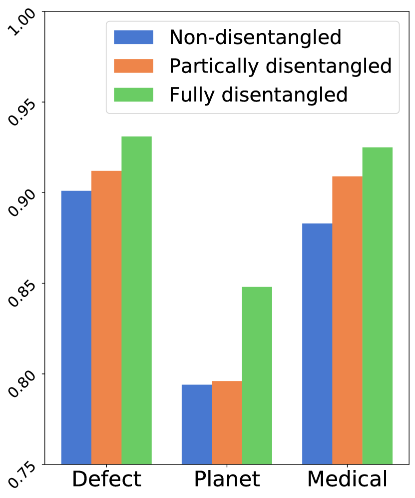
Figure 3: (Left) Disentangled vs. non-disentangled abnormality learning. The results are averaged over the datasets in each domain. (Right) AUC results of DRA using different reference set sizes ($\mathit{N}_{r}$). Each result is averaged over all data subsets per dataset.

Table 4: AUC results w.r.t. methods to create pseudo anomalies.

Anomaly Category		Augmentation			External
		CP-Scar	CP-Mix	CutMix	MVTec AD	LAG
Carpet	Color	0.743±0.142	0.967±0.048	0.886±0.042	0.615±0.028	0.711±0.041
	Cut	0.853±0.098	0.862±0.072	0.922±0.038	0.688±0.019	0.721±0.021
	Hole	0.809±0.033	0.955±0.024	0.947±0.016	0.712±0.015	0.823±0.020
	Metal	0.858±0.197	0.840±0.096	0.933±0.022	0.764±0.039	0.670±0.037
	Thread	0.987±0.013	0.988±0.011	0.989±0.004	0.966±0.003	0.968±0.005
	Mean	0.850±0.070	0.922±0.012	0.935±0.013	0.749±0.006	0.779±0.017
AITEX	Broken_end	0.584±0.127	0.750±0.115	0.693±0.099	0.793±0.043	0.722±0.072
	Broken_pick	0.616±0.111	0.671±0.082	0.760±0.037	0.603±0.017	0.584±0.034
	Cut_selvage	0.676±0.032	0.653±0.091	0.777±0.036	0.690±0.013	0.683±0.035
	Fuzzyball	0.639±0.056	0.582±0.067	0.701±0.093	0.743±0.053	0.588±0.112
	Nep	0.679±0.060	0.706±0.096	0.750±0.038	0.774±0.029	0.739±0.012
	Weft_crack	0.470±0.209	0.507±0.293	0.717±0.072	0.671±0.031	0.480±0.140
	Mean	0.611±0.064	0.645±0.070	0.733±0.009	0.712±0.010	0.633±0.049
ELPV	Mono	0.665±0.098	0.622±0.067	0.731±0.021	0.543±0.064	0.544±0.041
	Poly	0.755±0.006	0.807±0.085	0.800±0.064	0.749±0.052	0.808±0.056
	Mean	0.710±0.046	0.715±0.076	0.766±0.029	0.646±0.042	0.676±0.031
Hyper-Kvasir	Barretts	0.832±0.016	0.735±0.028	0.761±0.043	0.834±0.024	0.824±0.006
	B.-short-seg	0.827±0.054	0.719±0.049	0.695±0.030	0.839±0.038	0.835±0.021
	Esophagitis-a	0.832±0.024	0.751±0.023	0.763±0.070	0.811±0.031	0.881±0.035
	E.-b-d	0.805±0.035	0.749±0.060	0.782±0.028	0.847±0.017	0.837±0.009
	Mean	0.824±0.020	0.739±0.007	0.751±0.021	0.833±0.023	0.844±0.009

4.6 Sensitivity Analysis

Sensitivity w.r.t.  the Source of Pseudo Anomalies There are diverse ways to create pseudo anomalies, as shown in previous studies [26, 42, 54, 18] that focus on anomaly-free training data. We instead investigate the effect of these methods under our open-set supervised AD model DRA. We evaluate three data augmentation methods, including CutMix [67], CutPaste-Scar (CP-Scar) [26] and CutPaste-Mix (CP-Mix) that utilizes both CutMix and CP-Scar, and two outlier exposure methods that respectively use samples from MVTec AD [3] and medical dataset LAG [27] as the pseudo anomalies. When using MVTec AD, we remove the classes that overlap with the training/test data; LAG does not have any overlapping with our datasets. Since pseudo anomalies are used mainly to enhance the generalization to unseen anomalies, we focus on the four hard setting datasets in our ablation study in Tab. 3.

The results are shown in Tab. 4, from which it is clear that the data augmentation-based pseudo anomaly creation methods are generally more stable and much better than the external data-based methods on non-medical datasets. On the other hand, the external data method is more effective on medical datasets, since the augmentation methods often fail to properly simulate the lesions. The LAG dataset provides more application-relevant features and enables DRA to achieve the best results on Hyper-Kvasir.

Sensitivity w.r.t. the Reference Size in Latent Residual Abnormality Learning. Our latent residual abnormality learning head requires to sample a fixed number $\mathit{N}_{r}$ of normal training images as reference data. We evaluate the sensitivity of our method using different $\mathit{N}_{r}$ and report the AUC results in Fig. 3 (Right). Using one reference image is generally sufficient to learn the residual anomalies. Increasing the reference size to five helps further improve the detection performance, but increasing the size to ten is not consistently helpful. $\mathit{N}_{r}=5$ is generally recommended, which is the default setting in DRA in all our experiments.

5 Conclusions and Discussions

This paper proposes the framework of learning disentangled representations of abnormalities illustrated by seen anomalies, pseudo anomalies, and latent residual-based anomalies, and introduces the DRA model to effectively detect both seen and unseen anomalies. Our comprehensive results in Tabs. 7 and 2 justify that these three disentangled abnormality representations can complement each other in detecting the largely varying anomalies, substantially outperforming five SotA unsupervised and supervised anomaly detectors by a large margin, especially on the challenging cases, e.g., having only one training anomaly example, or detecting unseen anomalies.

The studied problem is largely under-explored, but it is very important in many relevant real-world applications. As shown by the results in Tabs. 7 and 2, there are still a number of major challenges requiring further investigation, e.g., generalization from smaller anomaly examples from fewer classes, of which our model and comprehensive results provide a good baseline and extensive benchmark results.

Appendix A Dataset Details

A.1 Key Statistics of Datasets

Tab. 5 summarizes the key statistics of these datasets. Below we introduce each dataset in detail. The normal samples in MVTec AD are split into training and test sets following the original settings. In other datasets, the normal samples are randomly split into training and test sets by a ratio of $3/1$.

MVTec AD [3] is a popular defect inspection benchmark that has 15 different classes, with each anomaly class containing one to several subclasses. In total the dataset contains 73 defective classes of fine-grained anomaly classes at the texture- or object-level.

AITEX [50] is a fabrics defect inspection dataset that has 12 defect classes, with pixel-level defect annotation. We crop the original $4096\times 256$ image to several $256\times 256$ patch image and relabel each patch by pixel-wise annotation.

SDD [53] is a defect inspection dataset images of defective production items with pixel-level defect annotation. We vertically and equally divide the original $500\times 1250$ image into three segment images and relabel each image by pixel-wise annotation.

ELPV [9] is a solar cells defect inspection dataset in electroluminescence imagery. It contains two defect classes depending on solar cells: mono- and poly-crystalline.

Optical [63] is a synthetic dataset for defect detection on industrial optical inspection. The artificially generated data is similar to real-world tasks.

Mastcam [22] is a novelty detection dataset constructed from geological image taken by a multispectral imaging system installed in Mars exploration rovers. It contains typical images and images of 11 novel geologic classes. Images including shorter wavelength (color) channel and longer wavelengths (grayscale) channel and we focus on shorter wavelength channel in this work.

BrainMRI [47] is a brain tumor detection dataset obtained by magnetic resonance imaging (MRI) of the brain.

HeadCT [47] is a brain hemorrhage detection dataset obtained by CT scan of head.

Hyper-Kvasir [5] is a large-scale open gastrointestinal dataset collected during real gastro- and colonoscopy procedures. It contains four main categories and 23 subcategories of gastro- and colonoscopy images. This work focuses on gastroscopy images with the anatomical landmark category as the normal samples and the pathological category as the anomalies.

Table 5: Key Statistics of Image Datasets. The first 15 datasets compose the MVTec AD dataset.

Dataset	Original Training	Original Test		Anomaly Data
	Normal	Normal	Anomaly	# Classes	Type
Carpet	280	28	89	5	Texture
Grid	264	21	57	5	Texture
Leather	245	32	92	5	Texture
Tile	230	33	84	5	Texture
Wood	247	19	60	5	Texture
Bottle	209	20	63	3	Object
Capsule	219	23	109	5	Object
Pill	267	26	141	7	Object
Transistor	213	60	40	4	Object
Zipper	240	32	119	7	Object
Cable	224	58	92	8	Object
Hazelnut	391	40	70	4	Object
Metal_nut	220	22	93	4	Object
Screw	320	41	119	5	Object
Toothbrush	60	12	30	1	Object
MVTec AD	3,629	467	1,258	73	-
AITEX	1,692	564	183	12	Texture
SDD	594	286	54	1	Texture
ELPV	1,131	377	715	2	Texture
Optical	10,500	3,500	2,100	1	Object
Mastcam	9,302	426	451	11	Object
BrainMRI	73	25	155	1	Medical
HeadCT	75	25	100	1	Medical
Hyper-Kvasir	2,021	674	757	4	Medical

Table 6: Download Link of Image Datasets.

Dataset	Link
MVTec AD	https://tinyurl.com/mvtecad
AITEX	https://tinyurl.com/aitex-defect
SDD	https://tinyurl.com/KolektorSDD
ELPV	https://tinyurl.com/elpv-crack
Optical	https://tinyurl.com/optical-defect
Mastcam	https://tinyurl.com/mastcam
BrainMRI	https://tinyurl.com/brainMRI-tumor
HeadCT	https://tinyurl.com/headCT-tumor
Hyper-Kvasir	https://tinyurl.com/hyper-kvasir

To provide some intuitive understanding of what the anomalies and normal samples look like, we present some examples of normal and anomalous images for each dataset in Fig. 4.

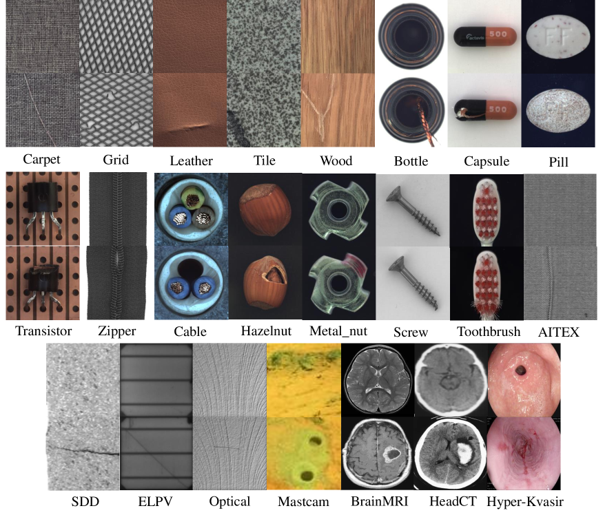
Figure 4: Examples of normal and anomalous images for each dataset. For each group of examples, the images on the top are normal, while the bottom ones are anomalous.

A.2 Dataset Split

We have two experiment protocols, including general and hard settings. For the general setting, the few labeled anomaly samples are randomly drawn from all possible anomaly classes in the test set per dataset. These sampled anomalies are then removed from the test data. For the hard setting, the anomaly example sampling is limited to be drawn from one single anomaly class only, and all anomaly samples in this anomaly class are removed from the test set to ensure that the test set contains only unseen anomaly classes. As labeled anomalies are difficult to obtain due to their rareness and unknowingness, in both settings we use only very limited labeled anomalies, i.e., with the number of the given anomaly examples respectively fixed to one and ten.

Additionally, to have a cross analysis of the results in the one-shot and ten-shot scenarios, the one anomaly example in the one-shot scenarios is randomly sampled from the ten sampled anomaly examples in the ten-shot scenarios, and they are all evaluated on exactly the same test data – the test data used in ten-shot scenarios. That is, the only difference between the one-shot and ten-shot scenarios is on the training anomaly examples.

Appendix B Implementation Details

In this section, we describe the implementation details of DRA and its competing methods.

B.1 Implementation of DRA

All input images are first resized to 448x448 or 224x224 according to the original resolution. We then use the ImageNet pre-trained ResNet-18 for the feature extraction network, which extracts a 512-dimensional feature map for an input image. This feature map is then fed to the subsequent abnormality/normality learning heads to learn disentangled abnormalities. The Patch-wise classifier in Plain Feature Learning adopted in the seen and pseudo abnormality learning heads is implemented by a 1x1 convolutional layer that yields the anomaly score of each vector in the feature map. The normality learning head utilizes a two-layer fully connected layer as the classifier, which first reduces a 512-dimensional feature vector to 256-dimensions and then yields anomaly scores. In the training phase, each input image is routed to different heads based on the labels, and each head computes the loss independently. All its heads are jointly trained using 30 epochs, with 20 iterations per epoch and a batch size of 48. Adam is used for the parameter optimization using an initial learning rate $10^{-3}$ with a weight decay of $10^{-2}$.

In the inference phase, each head yields anomaly scores for the target image simultaneously. Since all heads are optimized by the same loss function, the anomaly scores generated by each head have the same semantic, and so we calculate the sum of all the anomaly scores (and a negated normal score) as the final anomaly score. In addition, to solve the multi-scale problem, we use an image pyramid module with two-layer image pyramid, which obtains anomaly scores at different scales by inputting original images of various sizes, and calculates the mean value as the final anomaly score.

For the reference sets in Latent Residual Abnormality Learning, we found that mixing some generated pseudo-anomaly samples into normal samples can further improve performance. We speculate that adding pseudo-anomaly samples can get more challenging residual samples to help the network adapt to extreme cases. Therefore, we use the dataset mixed with normal and pseudo-abnormal samples as the reference set in the final implementation.

B.1.1 Loss Function

DRA can be optimized using different anomaly score loss functions. We use deviation loss [35] in our final implementation to optimize DRA, because it is generally more effective and stable than other popular loss functions, as shown in the experimental results in Section C.2. Particularly, a deviation loss optimizes the anomaly scoring network by a Gaussian prior score, with the deviation specified as a Z-score:

$$\mathit{dev}(\mathbf{x}_{i};\Theta)=\frac{g(f(\mathbf{x};\Theta_{f});\Theta_{g})-\mu_{\mathcal{R}}}{\sigma_{\mathcal{R}}},$$ (10)

where $\mu_{\mathcal{R}}$ and $\sigma_{\mathcal{R}}$ is the mean and standard deviation of the prior-based anomaly score set drawn from ${\cal N}(\mu,\sigma^{2})$. The deviation loss is specified using the contrastive loss [15] with the deviation plugged into:

$$\ell\big{(}\mathbf{x}_{i},\mu_{\mathcal{R}},\sigma_{\mathcal{R}};\Theta\big{)}=(1-y_{i})|\mathit{dev}(\mathbf{x}_{i};\Theta)|\\ +y_{i}\max\big{(}0,a-\mathit{dev}(\mathbf{x}_{i};\Theta)\big{)},$$ (11)

where $y=1$ indicate an anomaly and $y=0$ indicate a normal sample, and $a$ is equivalent to a Z-Score confidence interval parameter.

B.2 Implementation of Competing Methods

In the main text, we present five recent and closely related state-of-the-art (SOTA) competing methods. Here we introduce two additional competing methods. Following is the detailed description and implementation details of these seven methods:

KDAD [47] is an unsupervised deep anomaly detector based on multi-resolution knowledge distillation. We experiment with the code provided by its authors and report the results. Since KDAD is unsupervised, it is trained with normal data only, but it is evaluated on exactly the same test data as DRA.

DevNet [37, 35] is a supervised deep anomaly detector based on a prior-based deviation. The results we report are based on the implementation provided by its authors.

FLOS [28] is a deep imbalanced classifier that learns a binary classification model using the class-imbalance-sensitive loss – focal loss. The implementation of FLOS is also taken from [35], which replaces the loss function of DevNet with the focal loss.

SAOE is a deep out-of-distribution detector that utilizes pseudo anomalies from both data augmentation-based and outlier exposure-based methods. Motivated by the success of using pseudo anomalies to improve anomaly detection in recent studies [54, 26], SAOE is implemented by learning both seen and pseudo abnormalities through a multi-class (i.e., normal class, seen anomaly class, and pseudo anomaly class) classification head using the plain feature learning method as in DRA. In addition to this multi-class classification, the outlier exposure module [18] in SAOE is implemented according to its authors, in which the MVTec AD [3] or LAG [27] dataset is used as external data. In all our experiments we removed the related data from the outlier data that has any overlapping with the target data to avoid data leakage.

MLEP [30] is a deep open set anomaly detector based on margin learning embedded prediction. The original MLEP is designed for open set video anomaly detection, and we adapt it to image tasks by modifying the backbone network and training settings to be consistent with DRA.

Deep SAD [45] is a supervised deep anomaly detector that extends Deep SVDD [44] by using a few labeled anomalies and normal samples to learn more compact one-class descriptors. Particularly, it adds a new marginal constraint to the original Deep SVDD that enforces a large margin between labeled anomalies and the one-class center in latent space. The implementation of DeepSAD is taken from the original authors.

MINNS [62] is a deep multiple instance classification model, which is implemented based on [35].

Table 7: AUC results (mean±std) of DRA and two additional competing methods under the general setting. All methods are trained using ten random anomaly examples, with the best results are highlighted.

Dataset	$|\mathcal{C}|$	DeepSAD	MINNS	DRA (Ours)
Carpet	5	0.791±0.011	0.876±0.015	0.940±0.027
Grid	5	0.854±0.028	0.983±0.016	0.987±0.009
Leather	5	0.833±0.014	0.993±0.007	1.000±0.000
Tile	5	0.888±0.010	0.980±0.003	0.994±0.006
Wood	5	0.781±0.001	0.998±0.004	0.998±0.001
Bottle	3	0.913±0.002	0.995±0.007	1.000±0.000
Capsule	5	0.476±0.022	0.905±0.013	0.935±0.022
Pill	7	0.875±0.063	0.913±0.021	0.904±0.024
Transistor	4	0.868±0.006	0.889±0.032	0.915±0.025
Zipper	7	0.974±0.005	0.981±0.011	1.000±0.000
Cable	8	0.696±0.016	0.842±0.012	0.909±0.011
Hazelnut	4	1.000±0.000	1.000±0.000	1.000±0.000
Metal_nut	4	0.860±0.053	0.984±0.002	0.997±0.002
Screw	5	0.774±0.081	0.932±0.035	0.977±0.009
Toothbrush	1	0.885±0.063	0.810±0.086	0.826±0.021
MVTec AD	-	0.830±0.009	0.939±0.011	0.959±0.003
AITEX	12	0.686±0.028	0.813±0.030	0.893±0.017
SDD	1	0.963±0.005	0.961±0.016	0.991±0.005
ELPV	2	0.722±0.053	0.788±0.028	0.845±0.013
Optical	1	0.558±0.012	0.774±0.047	0.965±0.006
Mastcam	11	0.707±0.011	0.803±0.031	0.848±0.008
BrainMRI	1	0.850±0.016	0.943±0.031	0.970±0.003
HeadCT	1	0.928±0.005	0.984±0.010	0.972±0.002
Hyper-Kvasir	4	0.719±0.032	0.647±0.051	0.834±0.004

Appendix C Additional Empirical Results

C.1 Additional Comparison Results

General Setting. We report the results of DRA and two additional competing methods under general setting in Tab 7. Our method achieves the best AUC performance in eight of the nine datasets and the close-to-best AUC performance in the another dataset. In the eight best-performing datasets, our method improves AUC by 2% to 19.1% over the best competing method.

Hard Setting. Tab. 8 shows the results of DRA and two additional competing methods under the hard setting. Our method performs best on most of the data subsets and achieves the best AUC performance on five of the six datasets at the dataset level. Our method improves from 9.2% to 24.4% over the suboptimal method in the other five datasets.

The experimental results in both settings show the superiority of our method compared to Deep SAD and MINNS.

Table 8: AUC results of DRA and two additional competing methods under the hard setting, where models are trained with one known anomaly class and tested to detect the rest of all other anomaly classes. Each data subset is named by the known anomaly class.

Module		DeepSAD	MINNS	DRA (Ours)
Carpet	Color	0.736±0.007	0.767±0.011	0.886±0.042
	Cut	0.612±0.034	0.694±0.068	0.922±0.038
	Hole	0.576±0.036	0.766±0.007	0.947±0.016
	Metal	0.732±0.042	0.789±0.097	0.933±0.022
	Thread	0.979±0.000	0.982±0.008	0.989±0.004
	Mean	0.727±0.011	0.800±0.022	0.935±0.013
Metal_nut	Bent	0.821±0.023	0.868±0.033	0.990±0.003
	Color	0.707±0.028	0.985±0.018	0.967±0.011
	Flip	0.602±0.020	1.000±0.000	0.913±0.021
	Scratch	0.654±0.004	0.978±0.000	0.911±0.034
	Mean	0.696±0.012	0.958±0.008	0.945±0.017
AITEX	Broken_end	0.442±0.029	0.708±0.103	0.693±0.099
	Broken_pick	0.614±0.039	0.565±0.018	0.760±0.037
	Cut_selvage	0.523±0.032	0.734±0.012	0.777±0.036
	Fuzzyball	0.518±0.023	0.534±0.058	0.701±0.093
	Nep	0.733±0.017	0.707±0.059	0.750±0.038
	Weft_crack	0.510±0.058	0.544±0.183	0.717±0.072
	Mean	0.557±0.014	0.632±0.023	0.733±0.009
ELPV	Mono	0.554±0.063	0.557±0.010	0.731±0.021
	Poly	0.621±0.006	0.770±0.032	0.800±0.064
	Mean	0.588±0.021	0.663±0.015	0.766±0.029
Mastcam	Bedrock	0.474±0.038	0.419±0.025	0.658±0.021
	Broken-rock	0.497±0.054	0.687±0.015	0.649±0.047
	Drill-hole	0.494±0.013	0.651±0.035	0.725±0.005
	Drt	0.586±0.012	0.705±0.043	0.760±0.033
	Dump-pile	0.565±0.046	0.697±0.022	0.748±0.066
	Float	0.408±0.022	0.635±0.073	0.744±0.073
	Meteorite	0.489±0.010	0.551±0.018	0.716±0.004
	Scuff	0.502±0.010	0.502±0.040	0.636±0.086
	Veins	0.542±0.017	0.577±0.013	0.620±0.036
	Mean	0.506±0.009	0.603±0.016	0.695±0.004
Hyper-Kvasir	Barretts	0.672±0.017	0.679±0.009	0.824±0.006
	B.-short-seg	0.666±0.012	0.608±0.064	0.835±0.021
	Esophagitis-a	0.619±0.027	0.665±0.045	0.881±0.035
	E.-b-d	0.564±0.006	0.480±0.043	0.837±0.009
	Mean	0.630±0.009	0.608±0.014	0.844±0.009

C.2 Sensitivity w.r.t. Loss Function

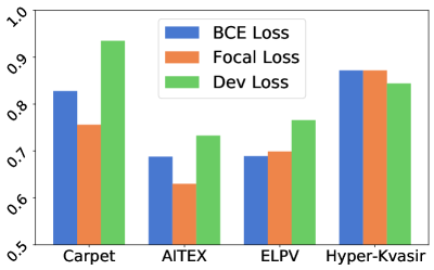
Figure 5: The AUC performance of our proposed method using different loss functions under the hard setting. We report the averaged results over all data subsets per dataset.

In our paper, we use the deviation loss [35] in all our four heads by default. Here we vary the use of the loss function and analyze the impact of the loss function on the performance of anomaly detection. Any related binary classification loss functions may be used for training all the four heads of DRA. We evaluate the applicability of two additional popular loss functions, including binary cross-entropy loss and focal loss, in addition to deviation loss. The results are reported in Fig. 5, where all results are the averaged AUC of three independent runs of the experiments. In general, the deviation loss function, which is specifically designed for anomaly detection, has clear superiority on most cases. The two classification losses perform better on the medical dataset Hyper-Kvasir. Based on such empirical findings, the deviation loss function is generally recommended in DRA.

C.3 Cross-domain Anomaly Detection

An interesting extension area of open-set anomaly detection is cross-domain anomaly detection, aiming at training detection models on a source domain to detect anomalies on datasets from a target domain different from the source domain. To demonstrate potential of our method in such setting, we report cross-domain AD results of our model DRA on all five texture anomaly datasets in MVTec AD in Tab. 9. DRA is trained on one of five datasets (source domain) and in fine-tuned with 10 epochs on the other four datasets (target domains) using normal samples only. The results show that the domain-adapted DRA significantly outperforms the SOTA unsupervised method KDAD that is directly trained on the target domain. This demonstrates some promising open-domain performance of DRA.

Table 9: AUC results of domain-adapted DRA and unsupervised method KDAD in texture datasets. The top row is the source domain and the left column is the target domain.

	carpet	grid	leather	tile	wood	KDAD
carpet	-	0.833	0.921	0.930	0.917	0.774
grid	0.983	-	0.924	0.940	0.916	0.749
leather	0.988	0.998	-	0.994	1.000	0.948
tile	0.917	0.971	0.958	-	0.955	0.911
wood	0.993	0.985	0.972	0.948	-	0.940

Appendix D Failure Cases

Although DRA shows competitive results on most datasets, it still fails on individual datasets; the most notable is the toothbrush dataset. After in-depth research and analysis of the results, we believe the failure of the toothbrush dataset is mainly due to its small size of normal samples (60 normal samples, see Tab. 5). Due to the more complex architecture, DRA often requires a relatively larger set of normal training samples to learn the disentangled abnormalities, while simpler methods like FLOS and SAOE that perform mainly binary classification do not have this requirement and work better on this dataset. In practice, we need to pay attention to the available data size of the target task, and apply a lightweight network in DRA instead when facing small-scale tasks.

References

- [1] Abhijit Bendale and Terrance E Boult. Towards open set deep networks. In Proc. IEEE Conf. Comp. Vis. Patt. Recogn., pages 1563–1572, 2016.
- [2] Liron Bergman and Yedid Hoshen. Classification-based anomaly detection for general data. In Proc. Int. Conf. Learn. Representations, 2020.
- [3] Paul Bergmann, Michael Fauser, David Sattlegger, and Carsten Steger. Mvtec ad – a comprehensive real-world dataset for unsupervised anomaly detection. In Proc. IEEE Conf. Comp. Vis. Patt. Recogn., June 2019.
- [4] Paul Bergmann, Michael Fauser, David Sattlegger, and Carsten Steger. Uninformed students: Student-teacher anomaly detection with discriminative latent embeddings. In Proc. IEEE Conf. Comp. Vis. Patt. Recogn., June 2020.
- [5] Hanna Borgli, Vajira Thambawita, Pia H Smedsrud, Steven Hicks, Debesh Jha, Sigrun L Eskeland, Kristin Ranheim Randel, Konstantin Pogorelov, Mathias Lux, Duc Tien Dang Nguyen, et al. Hyperkvasir, a comprehensive multi-class image and video dataset for gastrointestinal endoscopy. Scientific Data, 7(1):1–14, 2020.
- [6] Paula Branco, Luís Torgo, and Rita Ribeiro. A survey of predictive modeling on imbalanced domains. ACM Computing Surveys, 49(2):1–50, 2016.
- [7] Raghavendra Chalapathy, Aditya Krishna Menon, and Sanjay Chawla. Anomaly detection using one-class neural networks. arXiv preprint arXiv:1802.06360, 2018.
- [8] Yuanhong Chen, Yu Tian, Guansong Pang, and Gustavo Carneiro. Deep one-class classification via interpolated gaussian descriptor. In Proc. AAAI Conf. Artificial Intell., 2022.
- [9] Sergiu Deitsch, Vincent Christlein, Stephan Berger, Claudia Buerhop-Lutz, Andreas Maier, Florian Gallwitz, and Christian Riess. Automatic classification of defective photovoltaic module cells in electroluminescence images. Solar Energy, 185:455–468, 2019.
- [10] Giancarlo Di Biase, Hermann Blum, Roland Siegwart, and Cesar Cadena. Pixel-wise anomaly detection in complex driving scenes. In Proc. IEEE Conf. Comp. Vis. Patt. Recogn., pages 16918–16927, 2021.
- [11] Mariana-Iuliana Georgescu, Antonio Barbalau, Radu Tudor Ionescu, Fahad Shahbaz Khan, Marius Popescu, and Mubarak Shah. Anomaly detection in video via self-supervised and multi-task learning. In Proc. IEEE Conf. Comp. Vis. Patt. Recogn., pages 12742–12752, 2021.
- [12] Izhak Golan and Ran El-Yaniv. Deep anomaly detection using geometric transformations. In Proc. Advances in Neural Inf. Process. Syst., pages 9758–9769, 2018.
- [13] Dong Gong, Lingqiao Liu, Vuong Le, Budhaditya Saha, Moussa Reda Mansour, Svetha Venkatesh, and Anton van den Hengel. Memorizing normality to detect anomaly: Memory-augmented deep autoencoder for unsupervised anomaly detection. In Proc. IEEE Int. Conf. Comp. Vis., pages 1705–1714, 2019.
- [14] Nico Görnitz, Marius Kloft, Konrad Rieck, and Ulf Brefeld. Toward supervised anomaly detection. J. Artificial Intelligence Research, 46:235–262, 2013.
- [15] R. Hadsell, S. Chopra, and Y. LeCun. Dimensionality reduction by learning an invariant mapping. In Proc. IEEE Conf. Comp. Vis. Patt. Recogn., volume 2, pages 1735–1742, 2006.
- [16] Haibo He and Edwardo A Garcia. Learning from imbalanced data. IEEE T. Knowledge and Data Engineering, 21(9):1263–1284, 2009.
- [17] Dan Hendrycks and Kevin Gimpel. A baseline for detecting misclassified and out-of-distribution examples in neural networks. In Proc. Int. Conf. Learn. Representations, 2017.
- [18] Dan Hendrycks, Mantas Mazeika, and Thomas Dietterich. Deep anomaly detection with outlier exposure. In Proc. Int. Conf. Learn. Representations, 2019.
- [19] Jinlei Hou, Yingying Zhang, Qiaoyong Zhong, Di Xie, Shiliang Pu, and Hong Zhou. Divide-and-assemble: Learning block-wise memory for unsupervised anomaly detection. In Proc. IEEE Int. Conf. Comp. Vis., pages 8791–8800, October 2021.
- [20] Rui Huang and Yixuan Li. Mos: Towards scaling out-of-distribution detection for large semantic space. In Proc. IEEE Conf. Comp. Vis. Patt. Recogn., pages 8710–8719, 2021.
- [21] Radu Tudor Ionescu, Sorina Smeureanu, Bogdan Alexe, and Marius Popescu. Unmasking the abnormal events in video. In Proc. IEEE Int. Conf. Comp. Vis., pages 2895–2903, 2017.
- [22] Hannah R Kerner, Kiri L Wagstaff, Brian D Bue, Danika F Wellington, Samantha Jacob, Paul Horton, James F Bell, Chiman Kwan, and Heni Ben Amor. Comparison of novelty detection methods for multispectral images in rover-based planetary exploration missions. Data Mining and Knowledge Discovery, 34(6):1642–1675, 2020.
- [23] Nima Khakzad, Faisal Khan, and Paul Amyotte. Major accidents (gray swans) likelihood modeling using accident precursors and approximate reasoning. Risk analysis, 35(7):1336–1347, 2015.
- [24] Alex Krizhevsky, Geoffrey Hinton, et al. Learning multiple layers of features from tiny images. 2009.
- [25] Yann LeCun, Léon Bottou, Yoshua Bengio, and Patrick Haffner. Gradient-based learning applied to document recognition. Proceedings of the IEEE, 86(11):2278–2324, 1998.
- [26] Chun-Liang Li, Kihyuk Sohn, Jinsung Yoon, and Tomas Pfister. Cutpaste: Self-supervised learning for anomaly detection and localization. In Proc. IEEE Conf. Comp. Vis. Patt. Recogn., pages 9664–9674, 2021.
- [27] Liu Li, Mai Xu, Xiaofei Wang, Lai Jiang, and Hanruo Liu. Attention based glaucoma detection: A large-scale database and cnn model. In Proc. IEEE Conf. Comp. Vis. Patt. Recogn., June 2019.
- [28] Tsung-Yi Lin, Priya Goyal, Ross Girshick, Kaiming He, and Piotr Dollár. Focal loss for dense object detection. In Proc. IEEE Int. Conf. Comp. Vis., pages 2980–2988, 2017.
- [29] Ziqian Lin, Sreya Dutta Roy, and Yixuan Li. Mood: Multi-level out-of-distribution detection. In Proc. IEEE Conf. Comp. Vis. Patt. Recogn., pages 15313–15323, June 2021.
- [30] Wen Liu, Weixin Luo, Zhengxin Li, Peilin Zhao, Shenghua Gao, et al. Margin learning embedded prediction for video anomaly detection with a few anomalies. In Proc. Int. Joint Conf. Artificial Intell., pages 3023–3030, 2019.
- [31] Ziwei Liu, Zhongqi Miao, Xiaohang Zhan, Jiayun Wang, Boqing Gong, and Stella X Yu. Large-scale long-tailed recognition in an open world. In Proc. IEEE Conf. Comp. Vis. Patt. Recogn., pages 2537–2546, 2019.
- [32] Philipp Liznerski, Lukas Ruff, Robert A. Vandermeulen, Billy Joe Franks, Marius Kloft, and Klaus-Robert Müller. Explainable deep one-class classification. In Proc. Int. Conf. Learn. Representations, 2021.
- [33] Amir Markovitz, Gilad Sharir, Itamar Friedman, Lihi Zelnik-Manor, and Shai Avidan. Graph embedded pose clustering for anomaly detection. In Proc. IEEE Conf. Comp. Vis. Patt. Recogn., June 2020.
- [34] Guansong Pang, Longbing Cao, Ling Chen, and Huan Liu. Learning representations of ultrahigh-dimensional data for random distance-based outlier detection. In Proc. ACM SIGKDD Int. Conf. Knowledge Discovery & Data Mining, pages 2041–2050, 2018.
- [35] Guansong Pang, Choubo Ding, Chunhua Shen, and Anton van den Hengel. Explainable deep few-shot anomaly detection with deviation networks. arXiv preprint arXiv:2108.00462, 2021.
- [36] Guansong Pang, Chunhua Shen, Longbing Cao, and Anton Van Den Hengel. Deep learning for anomaly detection: A review. ACM Computing Surveys, 54(2):1–38, 2021.
- [37] Guansong Pang, Chunhua Shen, and Anton van den Hengel. Deep anomaly detection with deviation networks. In Proc. ACM SIGKDD Int. Conf. Knowledge Discovery & Data Mining, pages 353–362, 2019.
- [38] Guansong Pang, Anton van den Hengel, Chunhua Shen, and Longbing Cao. Toward deep supervised anomaly detection: Reinforcement learning from partially labeled anomaly data. In Proc. ACM SIGKDD Int. Conf. Knowledge Discovery & Data Mining, pages 1298–1308, 2021.
- [39] Hyunjong Park, Jongyoun Noh, and Bumsub Ham. Learning memory-guided normality for anomaly detection. In Proc. IEEE Conf. Comp. Vis. Patt. Recogn., June 2020.
- [40] Pramuditha Perera, Ramesh Nallapati, and Bing Xiang. Ocgan: One-class novelty detection using gans with constrained latent representations. In Proc. IEEE Conf. Comp. Vis. Patt. Recogn., June 2019.
- [41] Pramuditha Perera and Vishal M Patel. Learning deep features for one-class classification. IEEE Transactions on Image Processing, 28(11):5450–5463, 2019.
- [42] Tal Reiss, Niv Cohen, Liron Bergman, and Yedid Hoshen. Panda: Adapting pretrained features for anomaly detection and segmentation. In Proc. IEEE Conf. Comp. Vis. Patt. Recogn., pages 2806–2814, 2021.
- [43] Jie Ren, Peter J Liu, Emily Fertig, Jasper Snoek, Ryan Poplin, Mark A DePristo, Joshua V Dillon, and Balaji Lakshminarayanan. Likelihood ratios for out-of-distribution detection. In Proc. Advances in Neural Inf. Process. Syst., 2019.
- [44] Lukas Ruff, Robert Vandermeulen, Nico Goernitz, Lucas Deecke, Shoaib Ahmed Siddiqui, Alexander Binder, Emmanuel Müller, and Marius Kloft. Deep one-class classification. In Proc. Int. Conf. Mach. Learn., pages 4393–4402, 2018.
- [45] Lukas Ruff, Robert A Vandermeulen, Nico Görnitz, Alexander Binder, Emmanuel Müller, Klaus-Robert Müller, and Marius Kloft. Deep semi-supervised anomaly detection. In Proc. Int. Conf. Learn. Representations, 2020.
- [46] Mohammad Sabokrou, Mohammad Khalooei, Mahmood Fathy, and Ehsan Adeli. Adversarially learned one-class classifier for novelty detection. In Proc. IEEE Conf. Comp. Vis. Patt. Recogn., pages 3379–3388, 2018.
- [47] Mohammadreza Salehi, Niousha Sadjadi, Soroosh Baselizadeh, Mohammad Hossein Rohban, and Hamid R Rabiee. Multiresolution knowledge distillation for anomaly detection. In Proc. IEEE Conf. Comp. Vis. Patt. Recogn., 2021.
- [48] Walter J Scheirer, Anderson de Rezende Rocha, Archana Sapkota, and Terrance E Boult. Toward open set recognition. IEEE Trans. Pattern Anal. Mach. Intell., 35(7):1757–1772, 2012.
- [49] Thomas Schlegl, Philipp Seeböck, Sebastian M Waldstein, Georg Langs, and Ursula Schmidt-Erfurth. f-anogan: Fast unsupervised anomaly detection with generative adversarial networks. Medical Image Analysis, 54:30–44, 2019.
- [50] Javier Silvestre-Blanes, Teresa Albero Albero, Ignacio Miralles, Rubén Pérez-Llorens, and Jorge Moreno. A public fabric database for defect detection methods and results. Autex Research Journal, 19(4):363–374, 2019.
- [51] Kihyuk Sohn, Chun-Liang Li, Jinsung Yoon, Minho Jin, and Tomas Pfister. Learning and evaluating representations for deep one-class classification. In Proc. Int. Conf. Learn. Representations, 2021.
- [52] Waqas Sultani, Chen Chen, and Mubarak Shah. Real-world anomaly detection in surveillance videos. In Proc. IEEE Conf. Comp. Vis. Patt. Recogn., pages 6479–6488, 2018.
- [53] Domen Tabernik, Samo Šela, Jure Skvarč, and Danijel Skočaj. Segmentation-Based Deep-Learning Approach for Surface-Defect Detection. Journal of Intelligent Manufacturing, May 2019.
- [54] Jihoon Tack, Sangwoo Mo, Jongheon Jeong, and Jinwoo Shin. Csi: Novelty detection via contrastive learning on distributionally shifted instances. Proc. Advances in Neural Inf. Process. Syst., 33:11839–11852, 2020.
- [55] Nassim Nicholas Taleb. The black swan: The impact of the highly improbable, volume 2. Random house, 2007.
- [56] Yu Tian, Yuyuan Liu, Guansong Pang, Fengbei Liu, Yuanhong Chen, and Gustavo Carneiro. Pixel-wise energy-biased abstention learning for anomaly segmentation on complex urban driving scenes. arXiv: Comp. Res. Repository, 2021.
- [57] Yu Tian, Guansong Pang, Fengbei Liu, Yuanhong Chen, Seon Ho Shin, Johan W Verjans, Rajvinder Singh, and Gustavo Carneiro. Constrained contrastive distribution learning for unsupervised anomaly detection and localisation in medical images. In Proc. Int. Conf. Medical Image Computing and Computer Assisted Intervention, pages 128–140. Springer, 2021.
- [58] Shashanka Venkataramanan, Kuan-Chuan Peng, Rajat Vikram Singh, and Abhijit Mahalanobis. Attention guided anomaly localization in images. In Proc. Eur. Conf. Comp. Vis., pages 485–503. Springer, 2020.
- [59] Peng Wang, Lingqiao Liu, Chunhua Shen, Zi Huang, Anton van den Hengel, and Heng Tao Shen. What’s wrong with that object? identifying images of unusual objects by modelling the detection score distribution. In Proc. IEEE Conf. Comp. Vis. Patt. Recogn., pages 1573–1581, 2016.
- [60] Shenzhi Wang, Liwei Wu, Lei Cui, and Yujun Shen. Glancing at the patch: Anomaly localization with global and local feature comparison. In Proc. IEEE Conf. Comp. Vis. Patt. Recogn., pages 254–263, 2021.
- [61] Siqi Wang, Yijie Zeng, Xinwang Liu, En Zhu, Jianping Yin, Chuanfu Xu, and Marius Kloft. Effective end-to-end unsupervised outlier detection via inlier priority of discriminative network. In Proc. Advances in Neural Inf. Process. Syst., pages 5960–5973, 2019.
- [62] Xinggang Wang, Yongluan Yan, Peng Tang, Xiang Bai, and Wenyu Liu. Revisiting multiple instance neural networks. Pattern Recognition, 74:15–24, 2018.
- [63] M Wieler and T Hahn. Weakly supervised learning for industrial optical inspection. In DAGM Symposium, 2007.
- [64] Han Xiao, Kashif Rasul, and Roland Vollgraf. Fashion-mnist: a novel image dataset for benchmarking machine learning algorithms, 2017.
- [65] Jihun Yi and Sungroh Yoon. Patch SVDD: Patch-level svdd for anomaly detection and segmentation. In Proc. Asian Conf. Comp. Vis., 2020.
- [66] Zhongqi Yue, Tan Wang, Qianru Sun, Xian-Sheng Hua, and Hanwang Zhang. Counterfactual zero-shot and open-set visual recognition. In Proc. IEEE Conf. Comp. Vis. Patt. Recogn., pages 15404–15414, June 2021.
- [67] Sangdoo Yun, Dongyoon Han, Seong Joon Oh, Sanghyuk Chun, Junsuk Choe, and Youngjoon Yoo. Cutmix: Regularization strategy to train strong classifiers with localizable features. In Proc. IEEE Int. Conf. Comp. Vis., pages 6023–6032, 2019.
- [68] Alireza Zaeemzadeh, Niccolo Bisagno, Zeno Sambugaro, Nicola Conci, Nazanin Rahnavard, and Mubarak Shah. Out-of-distribution detection using union of 1-dimensional subspaces. In Proc. IEEE Conf. Comp. Vis. Patt. Recogn., pages 9452–9461, June 2021.
- [69] Muhammad Zaigham Zaheer, Jin-ha Lee, Marcella Astrid, and Seung-Ik Lee. Old is gold: Redefining the adversarially learned one-class classifier training paradigm. In Proc. IEEE Conf. Comp. Vis. Patt. Recogn., pages 14183–14193, 2020.
- [70] Muhammad Zaigham Zaheer, Arif Mahmood, Marcella Astrid, and Seung-Ik Lee. Claws: Clustering assisted weakly supervised learning with normalcy suppression for anomalous event detection. In Proc. Eur. Conf. Comp. Vis., pages 358–376. Springer, 2020.
- [71] Jianpeng Zhang, Yutong Xie, Guansong Pang, Zhibin Liao, Johan Verjans, Wenxing Li, Zongji Sun, Jian He, Yi Li, Chunhua Shen, and Yong Xia. Viral pneumonia screening on chest x-rays using confidence-aware anomaly detection. IEEE T. Medical Imaging, 40(3):879–890, 2021.
- [72] Chong Zhou and Randy C Paffenroth. Anomaly detection with robust deep autoencoders. In Proc. ACM SIGKDD Int. Conf. Knowledge Discovery & Data Mining, pages 665–674, 2017.
- [73] Da-Wei Zhou, Han-Jia Ye, and De-Chuan Zhan. Learning placeholders for open-set recognition. In Proc. IEEE Conf. Comp. Vis. Patt. Recogn., pages 4401–4410, 2021.
- [74] Kang Zhou, Yuting Xiao, Jianlong Yang, Jun Cheng, Wen Liu, Weixin Luo, Zaiwang Gu, Jiang Liu, and Shenghua Gao. Encoding structure-texture relation with p-net for anomaly detection in retinal images. In Proc. Eur. Conf. Comp. Vis., pages 360–377. Springer, 2020.