MolGenSurvey:
A Systematic Survey in Machine Learning Models for Molecule Design

Abstract

Molecule design is a fundamental problem in molecular science and has critical applications in a variety of areas, such as drug discovery, material science, etc. However, due to the large searching space, it is impossible for human experts to enumerate and test all molecules in wet-lab experiments. Recently, with the rapid development of machine learning methods, especially generative methods, molecule design has achieved great progress by leveraging machine learning models to generate candidate molecules. In this paper, we systematically review the most relevant work in machine learning models for molecule design. We start with a brief review of the mainstream molecule featurization and representation methods (including 1D string, 2D graph, and 3D geometry) and general generative methods (deep generative and combinatorial optimization methods). Then we summarize all the existing molecule design problems into several venues according to the problem setup, including input, output types and goals. Finally, we conclude with the open challenges and point out future opportunities of machine learning models for molecule design in real-world applications.

1 Introduction

Designing new molecules has been a long-standing challenge in molecular science and has critical applications in many domains such as drug discovery and material design [1]. Traditional methods, e.g., high-throughput screening (HTS) technologies, search over existing molecule databases but rely heavily on enumeration, thus are very time-consuming and laborious [2, 3]. On the other hand, the number of the drug-like molecules is large as estimated to be $10^{60}$ [4] and it is computationally prohibitive to enumerate all the possible molecules. To address the issue, machine learning approaches have been proposed to narrow down the searching space of molecules and explore the chemical space intelligently.

Among different types of machine learning approaches, generative methods offer a promising direction for the automated design of molecules with desired properties such as synthesis accessibility, binding affinity, etc. A wide range of generative methods has been proposed for molecule design, mainly in two types, (1) deep generative models and (2) combinatorial optimization methods. Deep generative models (DGMs) usually map molecules into a continuous latent space while combinatorial optimization methods directly search over the discrete chemical space.

Another key component of molecule design in machine learning is how the molecules are represented which includes 1D string, 2D graph, 3D geometry, etc. Early attempts formulate the molecule design as a 1D string generation problem and represent molecules as simplified molecular-input line-entry system (SMILES) strings. However, the validity of the generated SMILES string is not guaranteed [5]. To address the issues, other string featurization methods are explored, including an alternative string representation, self-referencing embedded strings (SELFIES) [6], which enforces string validity by design. With the emergence of graph representation learning, 2D graph representation has been introduced for molecule design and soon become a research hot spot as 2D graph is expected to carry richer structure information than 1D string.

Despite the success achieved in 1D and 2D molecule generation, molecules are naturally 3D structures and 3D conformations of molecules are crucial to many real-world applications such as structured-based drug design. However, representing a molecule by its 3D geometry is a nontrivial problem as it has to respect symmetry in 3D space such as translation- and rotation-equivariance. With the recent advances on geometric deep learning [7], efforts have been put to study representing molecules by 3D geometry and the wave has led to advances in molecule design in 3D space.

Nevertheless, one of the biggest challenges that stifles the progress of machine learning for molecule design is the fast-growing and not well-organized literature. Specifically, many different types of featurization and generative methods have been proposed for different types of molecule design tasks while the boundaries among them are not clearly specified. Although many recent efforts have been put to review the literature of machine learning models for molecule design, most of them only focus on part of the literature in terms of generative methods and tasks [8, 9, 10, 11, 12, 13, 14]. To the best of our knowledge, we are the first to provide a comprehensive review on machine learning approaches (both deep generative and combinatorial optimization methods) for 1D/2D/3D molecule design under a variety of task settings. Specifically, we present a mind map that drives the key taxonomies in molecule design tasks and unifies the task settings via the input/output types, and goals. The main contributions are summarized as follows:

• Review of Methods. Section 2 and 3 gather and categorize the mainstream molecule representation and general generation approaches, respectively.

• Review of Tasks. Section 4 elaborates the existing molecule design tasks and unifies them into a highly structured mindmap/table.

• Review of Experiments. Section 5 specifies the empirical setups of molecule design, including evaluation metrics, available datasets, oracles (usually molecular properties), etc.

• Challenges and Opportunities. Section 6 identifies open challenges and opportunities along the research direction for molecule design, paving the way for the future of molecule design with machine learning models.

2 Molecule Structure and Representation Learning

In this section, we introduce the mainstream featurization and representation learning methods for molecules. The three prevalent features adopted in molecule generation tasks are 1D string description, 2D molecular graph, and 3D molecular geometry. One example of the three features on a specific molecule (IUPAC: methylbenzene) is given in Footnote 1.

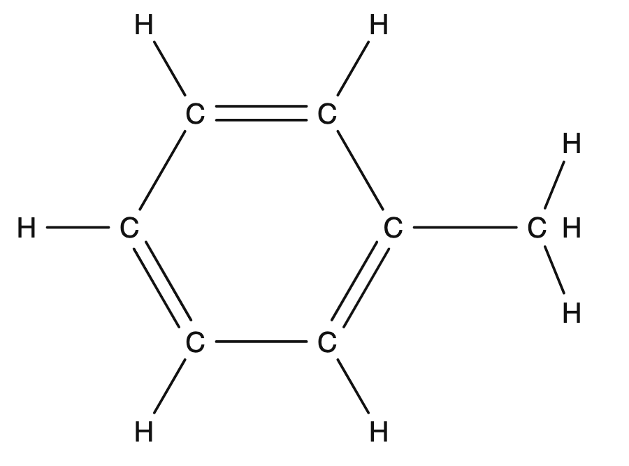
(a) 2D Molecular Graph

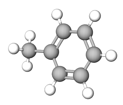
(b) 3D molecular Geometry

Figure 1: Four data structures on an example molecule. The 1D SMILES string is Cc1ccccc1, and the 1D SELFIES string is [C][C][=C][C][=C][C][=C][Ring1][=Branch1]. Figures 1(a) and 1(b) are the 2D and 3D molecular Geometry respectively.

2.1 1D String Description

The 1D string description is to extract molecules into a 1D string following certain domain-specific rules. The mainstream 1D string descriptions used for molecule generation include simplified molecular-input line-entry system (SMILES) [15] and self-referencing embedded strings (SELFIES) [16]. SMILES is well-known for its simplicity in denoting molecules as strings by following rules like adjacent atoms are assumed to be connected by a single or aromatic bond and branches are specified in parentheses, etc. However, one major limitation is that a significant fraction of SMILES strings are invalid. To avoid this, SELFIES augments the rules on handling branches and rings and thus it can achieve 100% validity.

We want to acknowledge that there exist other variants of 1D string descriptions, including International Chemical Identifier (InChI) [17], SMILES Arbitrary Target Specification (SMARTS) [18]; yet, SMILES and SELFIES are the two most commonly-used for molecule generation tasks.

Representation methods. For molecular string representation, existing work considers advanced representation methods from other domains, including convolutional neural network (CNN) [19], recurrent neural network (RNN) [20, 21, 22], and Transformer [23, 24, 25].

2.2 2D Molecular Graph

A large fraction of molecules can be naturally treated as 2D graphs: the atoms and bonds are nodes and edges in the graph, respectively. One example is given in Figure 1(a). Such featurization method has brought wide explorations in the structured data representation and related applications.

Representation methods. Graph neural network (GNN) is leveraged for 2D molecular graph representation. The high-level idea can be summarized into the message-passing neural network (MPNN) framework [26]: it updates each node’s representation by aggregating information from its neighborhood; by repeating this for $K$ steps, then each node’s final representations can reveal the information in the $K$-hop neighborhood. Generally, graph application is a broad field where certain GNNs [27, 28, 29] are originally proposed to solve other structured data, e.g., social network and citation network. Specifically for the molecular graph representation, NEF [30] is the first to apply GNN for property prediction, and more recent works have considered different aspects for improving the expressiveness of GNNs. Weave [31] explicitly models both the node- and edge-level representation. D-MPNN [32] and CMPNN [33] explicitly add the direction information in message passing. PNA [34] considers various aggregation methods during message passing. N-Gram Graph [35], on the other hand, proposes the walk-based GNN that can alleviate the over-squashing issue [36] in the MPNN-based GNN. Another big track is motivated by the recent success of the attention module in the NLP and vision domains [37, 38, 39]. To adapt it to molecular graphs, recent works utilize the attention to better capture the correlation at node-, subgraph-, and graph-level, including GAT [40], AttentiveFP [41], GTransformer [42], AWARE [43], and Graphormer [44].

2.3 3D molecular Geometry

Essentially, most molecule are not static, but instead in continual motion on a potential energy surface [45], characterized by different conformations, and the 3D structures at the local minima on this surface are named conformer. More concretely, we can view it as a sets of nodes in the 3D Euclidean space, as displayed in Figure 1(b).

Representation methods. Recent work on representing the 3D molecular Geometry assumes that if the learned representation is E(3)- or SE(3)-equivariant to a set of transformations, then such representation can reveal better expressiveness. This research line includes SchNet [47], OrbNet [48], DimeNet [49, 50], TFN [51], SE(3)-Transformer [51], EGNN [52], SpinConv [53], SphereNet [54], EVFN [55], UNiTE [56], SEGNN [57], PaiNN [58], and GemNet [59].

2.4 Other Molecular Featurization Methods

There also exist other molecule featurization and representation methods, yet they are not fit or not being widely explored for molecule generation tasks. Here we may as well briefly list them for comprehensiveness.

Descriptors It is mainly obtained by hashing the sub-components of the molecule into a fixed-length vector. The representation methods on fingerprints include random forest, XGBoost, multi-layer perceptron, etc. Recent work [60, 21, 61, 62] have empirically verified the effectiveness of descriptors. However, due to the irreversible hashing operation, it cannot be directly utilized for generation tasks.

3D density map This represents molecules as the 3D volume occupied by each of the atoms [63]. The volume for each atom is usually a function of the atomic radius which makes it a sphere-like solid object. The density map is often stored in a 3D grid. 3D CNN is a typical neural network utilized to encode the 3D density map [64].

3D surface mesh This represents molecules by their surfaces with 3D meshes (e.g., polygon mesh). The mesh consists of a collection of nodes, edges, and faces that define the shape of the molecular surface. The 3D surface mesh is usually encoded by a geodesic Convolutional Neural Network [65] or 3D Graph Neural Network [47].

Chemical Images This extracts the molecules into 2D grid images, as known as the chemical images. Then standard CNNs [66, 67] are applied on it for representation. Yet, this hasn’t been explored for molecule generation tasks yet.

2.5 Summary

Input data featurization and the learned representation function are two key components for molecule generation. A lot of follow-up works are built on this, including multi-task learning [60, 68, 69, 70, 71], self-supervised learning [72, 73, 74, 75, 76], and few-shot learning [77, 78, 79]. In the following sections, we will see how different feature and representation methods may fit into the generative methods (Section 3) and molecule generation tasks (Section 4).

3 Generative Methods

There are two main venues for generative methods. The first one is deep generative models (DGMs), which aim at modeling the data distribution using deep learning models. The second one is combinatorial optimization methods (COMs) that better utilize the heuristic strategies for the target goal. Specifically for the structured data, the main difference between these two venues is that DGMs utilize the continuous latent representation, while the COMs are directly searching in the structured data space. More details are discussed below, and key notations are listed in Table I.

TABLE I: Key notations for generative methods.

Notation Description ${\bm{x}}$ data point (2D or 3D molecule) ${\bm{z}}$ latent representation For AR: $d$ # subcomponents of data point ${\bm{x}}$ $\bar{x}_{0},\bar{x}_{1},...,\bar{x}_{d-1}$ each subcomponent of data point ${\bm{x}}$ For NF: $K$ # latent representation ${\bm{z}}_{0},{\bm{z}}_{1},...,{\bm{z}}_{K}$ list of $K$ latent representations For diffusion model: $T$ # steps ${\bm{x}}_{1},{\bm{x}}_{2},...,{\bm{x}}_{T}$ $T$ latent samples

3.1 Deep Generative Models (DGMs)

3.1.1 Autoregressive Models (ARs)

For each data point ${\bm{x}}$, especially for structured data like a graph, we first assume it has $d$ subcomponents, and such subcomponents can have underlying dependence. For example, the subcomponents can be the pixels in images or nodes and bonds in molecular graphs. The autoregressive models (ARs) learn the joint distribution of ${\bm{x}}$ by factorizing it as the product of $d$ subcomponent likelihoods as below:

$$\small{p({\bm{x}})=\prod_{i=1}^{d}p(\bar{x}_{i}|\bar{x}_{1},\bar{x}_{2},...,\bar{x}_{i-1}).}$$ (1)

Here ARs define an ordering of variables $\bar{x}_{i}$ (either heuristically or with domain knowledge), and model the joint distribution in an autoregressive or sequential manner: predicting the next subcomponent based on the previous subcomponents. ARs have been widely-used in generation tasks, including recurrent neural network (RNN) [80, 81], PixelCNN [82], WaveNet [83], Transformer [37] and BERT [38].

3.1.2 Variational Autoencoders (VAEs)

Variational autoencoders (VAEs) [84] estimate a lower bound (a.k.a. evidence lower bound (ELBO)) of the likelihood $p({\bm{x}})$. VAEs introduce a proposal distribution $q({\bm{z}}|{\bm{x}})$ and the goal is to maximize the ELBO:

$$\log p({\bm{x}}) =\log\int_{\bm{z}}p({\bm{z}})p({\bm{x}}|{\bm{z}})d{\bm{z}}$$ (2)

$$\geq\mathbb{E}_{q({\bm{z}}|{\bm{x}})}\big{[}\log p({\bm{x}}|{\bm{z}})\big{]}-D_{KL}(q({\bm{z}}|{\bm{x}})||p({\bm{z}}))$$

$$\triangleq\text{ELBO}.$$

The first term on ELBO is also known as the reconstruction term. Classic VAEs [84] take ${\bm{x}}$ as either continuous or binary, where we often model this conditional term as Gaussian or Bernoulli distribution. This will lead to mean-squared error (MSE) or binary cross-entropy (BCE) for reconstruction.

The second term of Equation 2 is the KL-divergence term measuring the information loss when using $q({\bm{z}}|{\bm{x}})$ to approximate $p({\bm{z}})$. In VAEs, the standard Gaussian is often used as the prior, i.e., $p({\bm{z}})\sim\mathcal{N}(0,I)$. Such standard Gaussian implies that all the learned latent dimensions are expected to be diverse or disentangled. Following work, e.g., $\beta$-VAE [85], penalizes this KL-divergence regularizer term to encourage the more disentangled latent representation, such that [86] each single unit in the latent representation is sensitive to only certain factors.

Reparameterization trick. VAEs express ${\bm{z}}$ as a deterministic variable ${\bm{z}}=g(\epsilon,{\bm{x}})$, where $\epsilon$ is an auxiliary variable with independent marginal $p(\epsilon)$, and $g(\cdot)$ is the reconstruction function. Then ${\bm{z}}$ can be reparameterized as:

$${\bm{z}}=g_{\phi}({\bm{x}},\epsilon)=\mu_{{\bm{x}}}+\sigma_{{\bm{x}}}\odot\epsilon,$$ (3)

where $\odot$ is the element-wise product. This reparameterization trick allows us to calculate the gradient of the reconstruction function with lower variance.

3.1.3 Normalizing Flows (NFs)

The normalizing flows (NFs) aim at modeling the data distribution $p({\bm{x}})$ directly with an invertible and deterministic mapping. First NFs suppose ${\bm{x}}$ and ${\bm{z}}$ are two random variables with the same dimension, ${\bm{x}}\sim p({\bm{x}})$ and ${\bm{z}}\sim p({\bm{z}})$. There exists an invertible mapping between the two variables, i.e., ${\bm{x}}=f({\bm{z}})$ and ${\bm{z}}=f^{-1}({\bm{x}})$. Then according to the change of variable theorem, we can have

$$\small{p({\bm{x}})=p({\bm{z}})\Big{|}\text{det}\Big{(}\frac{df^{-1}({\bm{x}})}{d{\bm{x}}}\Big{)}\Big{|},}$$ (4)

where $\frac{df^{-1}({\bm{x}})}{d{\bm{x}}}$ is the Jacobian matrix and $\text{det}(\cdot)$ is the matrix determinant.

Based on  Equation 4, an NFs map a simple prior distribution $p_{0}({\bm{z}}_{0})$ to a complex data distribution $p({\bm{x}})$ by applying a sequence of invertible transformation functions. In other words, the NFs flow through a chain of $K$ transformations ${\bm{z}}_{0}\to{\bm{z}}_{1}\to...\to{\bm{z}}_{K}={\bm{x}}$. Thus, the data distribution can be computed as

$$\log p({\bm{x}}) =\log p_{K}({\bm{z}}_{K})$$ (5)

$$=\log p_{K-1}({\bm{z}}_{K-1})-\log\Big{|}\text{det}\Big{(}\frac{df_{K}({\bm{z}}_{K-1})}{d{\bm{z}}_{K-1}}\Big{)}\Big{|}$$

$$=...$$

$$=\log p_{0}({\bm{z}}_{0})-\sum_{i=1}^{K}\log\Big{|}\text{det}\Big{(}\frac{df_{i}({\bm{z}}_{i-1})}{d{\bm{z}}_{i-1}}\Big{)}\Big{|}.$$

Existing works, e.g., RealNVP [87], NICE [88], and Glow [89], judiciously design invertible transformations $f_{i}$, where the Jacobian determinant is simple to compute.

3.1.4 Generative Adversarial Networks (GANs)

The Generative Adversarial Networks (GANs) [90] is a likelihood-free deep generative model. GANs do not optimize the likelihood directly; instead, they aim at detecting the real data from fake data, i.e., they transform the generation problem into a binary classification problem.

There are two main components in GANs: one generator ($G$) and one discriminator ($D$). The generator generates data points to fool the discriminator, while the discriminator tries to distinguish the generated data from the actual data. The objective of GANs is:

$$\min_{G}\max_{D}\mathcal{L}(D,G)$$ (6)

$$= \,\mathbb{E}_{{\bm{x}}\sim p_{data}}[\log D({\bm{x}})]+\mathbb{E}_{{\bm{z}}\sim p({\bm{z}})}[\log(1-D(G({\bm{z}}))].$$

The training of GANs risks the modal and model collapse issue. To alleviate this, f-GAN [91] adopts the f-divergence for measuring distribution distance, where the f-divergence is a more general metric that covers other widely-used distances, including KL divergence and Jenson-Shannon divergence. An alternative is Wasserstein-GAN (WGAN) [92] which utilizes the Wasserstein distance for measuring the distance between distributions. Follow-up works, including StyleGAN [93] and StyleGAN2 [94], introduce certain inductive biases in the architecture design and have been widely adopted in the community.

3.1.5 Diffusion models

Diffusion models [95, 96] are inspired by non-equilibrium thermodynamics and can be split into the forward and backward diffusion processes. During the forward diffusion process, the diffusion models will gradually add noise to the data and the last-step data will follow an isotropic Gaussian. The reverse diffusion process will revert this process and construct the data from noise distribution.

More rigorously, we can define the forward process as from the actual data ${\bm{x}}_{0}\sim p({\bm{x}})$ to the random noise ${\bm{x}}_{T}$ with $T$ diffusion steps. Let us first assume that for the forward process, the Gaussian distribution is

$$q({\bm{x}}_{t}|{\bm{x}}_{t-1}) =\mathcal{N}({\bm{x}}_{t};\sqrt{1-\beta_{t}}{\bm{x}}_{t-1},\beta_{t}I),$$

where $\beta_{t}\in(0,1)$. Then the corresponding backward process is

$$p_{\theta}({\bm{x}}_{t-1}|{\bm{x}}_{t}) =\mathcal{N}({\bm{x}}_{t-1};\mu_{\theta}({\bm{x}}_{t},t),\Sigma_{\theta}({\bm{x}}_{t},t))$$

$$=\mathcal{N}({\bm{x}}_{t-1};\frac{1}{\sqrt{\alpha_{t}}}\big{(}{\bm{x}}_{t}-\frac{\beta_{t}}{\sqrt{1-\bar{\alpha}_{t}}}\epsilon\big{)},\frac{1-\bar{\alpha}_{t-1}}{1-\bar{\alpha}_{t}}\beta_{t}),$$

where $\epsilon\sim\mathcal{N}(0,I)$ follows the standard Gaussian, $\alpha_{t}=1-\beta_{t}$, and $\bar{\alpha}_{t}=\prod_{i=1}^{t}\alpha_{i}$. The objective is to estimate the variational lower bound (VLB) of the likelihood:

$$\log p({\bm{x}})\geq-\mathbb{E}_{q(x_{1:T}|x_{0})}[\log\frac{q(x_{1:T}|x_{0})}{p_{\theta}(x_{0:T})}]=-\mathcal{L}_{\text{VLB}}.$$

The VLB can be rewritten as:

$$\mathcal{L}_{\text{VLB}}=\underbrace{KL[q(x_{T}|x_{0})||p_{\theta}(x_{T})]}_{\mathcal{L}_{T}}$$

$$~{}~{}~{}+\sum_{t=2}^{T}\underbrace{KL[q(x_{t-1}|x_{t},x_{0})||p_{\theta}(x_{t-1}|x_{t})]}_{\mathcal{L}_{t-1}}\underbrace{-\mathbb{E}_{q}[\log p_{\theta}(x_{0}|x_{1})]}_{\mathcal{L}_{0}}.$$

Here $\mathcal{L}_{T}$ is a constant and can be ignored, and existing methods [96, 97] have been using a separate model for estimating $\mathcal{L}_{0}$. For $\{\mathcal{L}_{t-1}\}_{t=2}^{T}$, they adopt a neural network to approximate the conditionals during the reverse process, and reduce to the following objective function:

$$\small{\mathcal{L}_{t}=\mathbb{E}_{{\bm{x}}_{0},z}\Big{[}\|\epsilon_{t}-\epsilon_{\theta}(\sqrt{\bar{\alpha}_{t}}{\bm{x}}_{0}+\sqrt{1-\bar{\alpha}_{t}}\epsilon_{t},t)\|^{2}\Big{]}.}$$

Please also notice that the final objective function is equivalent to a family of score matching methods [98, 99], as will be introduced below.

3.1.6 Energy-Based Models (EBMs)

Energy-based models (EBMs) have a very flexible formulation, and its general form is:

$$\small{p({\bm{x}})=\frac{\exp(-E_{\theta}({\bm{x}}))}{A}=\frac{\exp(-E_{\theta}({\bm{x}}))}{\int_{{\bm{x}}}\exp(-E_{\theta}({\bm{x}}))d{\bm{x}}},}$$ (7)

where $E_{\theta}(\cdot)$ is the energy function, $\theta$ is the set of learnable parameters, and $A$ is the partition function. In EBMs, the bottleneck is the calculation of partition function $A$: it is computationally intractable due to the high cardinality of $\mathcal{X}$. Various methods have been proposed to handle this task, and the most widely-used ones include contrastive divergence [100], noise-contrastive estimation (NCE) [101], score matching (SM) [98]. Each method has been widely explored, and for more details, we refer to this comprehensive summary [102].

3.2 Combinatorial Optimization Methods (COMs)

Deep generative models (DGMs) usually require a large amount of data to learn, which may be infeasible in real scenarios. In contrast, combinatorial optimization methods (COMs) have less requirement on the amount of training data, while the trade-off is that algorithm designers need to call the oracles during the exploration to the chemical space [103, 104, 105, 106, 107]. We mainly discuss five categories in COMs, (1) reinforcement learning (RL); (2) genetic algorithm (GA); (3) Bayesian Optimization (BO); (4) Monte Carlo Tree Search (MCTS), and (5) MCMC sampling. However, to conduct a thorough exploration of the chemical space, we need intensive oracle calls in combinatorial-based methods. For example, when we want to optimize molecules’ Quantitative Estimate of Drug-likeness (QED) score during the generative process, we need to evaluate the QED score of the generated molecules to guide the next step actions (i.e., call QED oracle).

3.2.1 Reinforcement Learning (RL)

Reinforcement learning (RL) is usually formulated as a Markov Decision Process (MDP). RL has several basic concepts: state, action, transition, and reward. The state is denoted as $S$, action set is denoted as $A$. At the $t$-th step, the transition probability from state $s$ to state $s^{\prime}$ under action $a\in A$ is $P_{\theta}(s,s^{\prime})=P(s_{t+1}=s^{\prime}|s_{t}=s,a_{t}=a)$, where $\theta$ is usually parameterized by neural networks. $R_{a}(s,s^{\prime})$ is the reward after transition from $s$ to $s^{\prime}$ with action $a$. The goal of RL is to learn an optimal policy that maximizes the “reward”,

$$\small{\underset{\theta}{\arg\max}\sum_{t=1}^{T}R_{a_{t}}(s_{t},s_{t+1}).}$$ (8)

For molecule generation tasks, a state is usually defined as a partially generated molecule graph, action can be adding a substructure (either an atom or a bond or a ring) at a position, and reward can be the property of the partially generated molecule. Specifically, [108, 109, 110, 111] leverage policy gradient and domain-specific reward function to optimize the graph policy neural network; [103] leverages deep Q-network to conduct value learning, where a deep Q-network is trained to predict the future reward and during each step, the step with maximal expected reward is selected.

3.2.2 Genetic Algorithm (GA)

Genetic Algorithm (GA) starts from a mating pool (set of strings/graphs that serve as warm start) and requires mutation and crossover between parents (interaction between intermediates in the last iteration) to obtain the next generation, where the population in each iteration is called a generation; parent is the intermediate from the previous generation; crossover, also called recombination, combines the genetic information of two parents to generate new offspring, offsprings are generated by cloning an existing solution; mutation involves an arbitrary bit in a genetic sequence that will be flipped from its original state. A common method of the mutation operator involves generating a random variable for each bit in a sequence. Specifically, at the $t$-th generation (iteration), given a population of molecules, denoted as $\mathcal{P}^{(t-1)}$, we generate a bunch of offsprings (the set is denoted as $\mathcal{S}^{(t)}$) and select the most promising $K$ ($K$ molecules with highest objectives) as the population for the next generation (denoted as $\mathcal{P}^{(t)}$). It is defined as

$$\mathcal{S}^{(t)}=\text{MUTATION}\big{(}\mathcal{P}^{(t-1)}\big{)}\cup\text{CROSSOVER}\big{(}\mathcal{P}^{(t-1)}\big{)}.$$ (9)

$$\mathcal{P}^{(t)}=\text{top-K}\big{(}\mathcal{S}^{(t)}\big{)}.$$

Specifically, GuacaMol benchmark [112, 107] proves the superiority of (i) SMILES-based GA and (ii) molecular graph-based GA. GA+D [6] leverages SELFIES string as the features of molecule and designs a genetic algorithm enhanced by adversarial learning. The superiority of GA methods is also validated in a molecule generation benchmark that optimizes docking score [113].

3.2.3 Monte Carlo Tree Search (MCTS)

Besides, Monte Carlo Tree Search (MCTS) [112, 114] based approaches show its superiority in molecule optimization. Different from GA, MCTS can start from scratch (e.g., a single node). Then during each generation iteration, it locally and randomly searches each branch of intermediates and selects the most promising (e.g., with highest property scores) ones for the next iteration.

$$\mathcal{S}^{(t)}=\text{SEARCH-BRANCH}\big{(}\mathcal{P}^{(t-1)}\big{)},$$ (10)

$$\mathcal{P}^{(t)}=\text{top-K}\big{(}\mathcal{S}^{(t)}\big{)},$$

the process is similar to GA (Equation 9), where $\mathcal{P}^{(t)}$ is the population at the $t$-th iteration, and $\mathcal{S}^{(t)}$ is the set of all the intermediates generated at the $t$-th iteration.

3.2.4 Bayesian Optimization (BO)

Bayesian optimization (BO) is usually used to optimize objective functions that demand a long evaluation time (minutes or hours). It is best suited for optimization over continuous domains of less than 20 dimensions [115] and tolerates stochastic noise in function evaluations. BO has two key steps: (1) BO builds a surrogate for the objective and quantifies the uncertainty in that surrogate using a Bayesian machine learning technique, Gaussian process (GP) regression. Suppose in the $t$-th iteration, we have collected $t$ noisy evaluations, $D_{t}=\{\mathbf{x}_{i},y_{i}\}_{i=1}^{t}$, where $y_{i}=f(\mathbf{x}_{i})+\epsilon_{i}$ for iid Gaussian noise $\epsilon_{i}\in\mathcal{N}(0,\sigma^{2})$. A GP surrogate model utilizes a non-parametric regression of a particular smoothness controlled by a kernel $k:\mathcal{X}\times\mathcal{X}\xrightarrow[]{}\mathbb{R}$ measuring the similarity between two points. (2) It utilizes an acquisition function defined from the surrogate to decide where to sample. Specifically, acquisition function $\alpha_{t}:\mathcal{X}\xrightarrow[]{}\mathbb{R}$ measures the utility of making a new evaluation given the predictions of current surrogate model. Within the $t$-th iteration, BO maximizes the acquisition function via $\mathbf{x}^{(t+1)}=\underset{x\in\mathcal{X}}{\arg\max}\ \alpha_{t}(x)$. Representative BO works include  [116, 115, 117, 118, 119, 120]. Also, BO methods can be combined VAE and optimize the latent vectors of VAE [5, 121].

3.2.5 Markov Chain Monte Carlo (MCMC)

MCMC is designed for drawing samples from target distribution (denoted $\pi(\cdot)$) efficiently. In the $t$-th iteration, MCMC mainly contains two steps: (1) samples the state from proposal distribution, i.e., $x^{(t)}\sim Q(\cdot|x^{(t-1)})$; and (2) accepts/rejects the proposal with probability $\min\{1,\frac{\pi(x^{(t)})Q(x^{(t-1)}|x^{(t)})}{\pi(x^{(t-1)})Q(x^{(t)}|x^{(t-1)})}\}$.

[122, 123] formulate the generation task as an sampling problem. To be more concrete, suppose we have $K$ constraints/objectives (denoted as $O_{1},\cdots,O_{K}$) during the optimization procedures, then the target sampling distribution $\pi(\cdot)$ (i.e., the data space of interest) is formulated as

$$\small{\pi(Y)\propto\prod_{k=1}^{K}O_{k}(Y),}$$ (11)

where $Y$ is a valid data (like chemically valid molecule). Usually MCMC utilizes a pretrained proposal distribution for sampling (usually a pretrained Graph Neural Network), i.e., $Q(Y^{(t+1)}|Y^{(t)})$, where $Y^{(t)}$ is the data at the $t$-th iteration.

3.3 Other Approaches

Optimal Transport (OT) is introduced when matching between two groups of molecules, especially for the molecule conformation generation problem where each molecule has multiple associated conformations and OT provides a way to optimize the generative model via measuring the distance between two probability distributions.

Differentiable Learning formulate discrete molecules into differentiable formats and enable gradient-based continuous optimization on the molecules directly. DST [104] formulates it by directly optimizing through the graph representation of molecules.

TABLE II: The input, output, and the goal that we are interested in w.r.t. the generation phase. NA means the task is not meaningful.

Input, Output goal 1D String 2D Graph (small molecule) 3D Geometry (small molecule) None goal-free de novo 1D molecule generation de novo 2D molecule generation de novo 3D molecule generation goal-oriented de novo 1D molecule optimization de novo 2D molecule optimization de novo 3D molecule optimization 1D String goal-free NA NA de novo 3D conformation generation goal-oriented 1D molecule optimization NA NA 2D Graph (small molecule) goal-free NA NA de novo 3D conformation generation goal-oriented NA 2D molecule optimization de novo 3D molecule optimization 3D Geometry (small molecule) goal-free NA NA NA goal-oriented NA NA 3D molecule optimization 3D Geometry (large molecule) goal-free NA NA NA goal-oriented NA NA de novo binding-based 3D molecule generation 1D String/2D Graph (small molecule) + 3D Geometry (large molecule) goal-free NA NA NA goal-oriented NA NA de novo binding-pose conformation generation

TABLE III: 2D molecule generation.

Generative Task	Model	Input	Output	Generative Method
de novo 1D/2D molecule generation	SD-VAE [124]	None	SMILES	VAE
	GrammarVAE [125]	None	SMILES	VAE
	ChemVAE [5]	None	SMILES	VAE
	JT-VAE [121]	None	2D-Graph	VAE
	GraphVAE [126]	None	2D-Graph	VAE
	CGVAE [127]	None	2D-Graph	VAE
	SG-VAE [128]	None	SMILES	VAE
	GraphNVP [129]	None	2D-Graph	Flow
	MoFlow [130]	None	2D-Graph	Flow
	GraphAF [131]	None	2D-Graph	Flow+AR
	GraphDF [132]	None	2D-Graph	Flow+AR
	dcGAN [133]	None	Fingerprint	GAN
	Defactor [134]	None	2D-Graph	GAN
	ORGAN [135]	None	SMILES	GAN+RL
	MolGAN [136]	None	2D-Graph	GAN+RL
	MolecularRNN [137]	None	2D-Graph	AR
	SF-RNN [138]	None	SELFIES	AR
	GraphEBM [139]	None	2D-Graph	EBM
de novo 1D/2D molecule optimization	RNN-finetune [140]	None	SMILES	AR
	PCVAE [141, 142]	None	2D-Graph	VAE
	MDVAE [143]	None	2D-Graph	VAE
	GB-GA [112]	None	2D-Graph	GA
	GA+D [6]	None	SELFIES	GA
	EDM [144]	None	SMILES	GA
	JANUS [145]	None	SELFIES	GA
	MolDQN [103]	None	2D-Graph	RL
	RationaleRL [109]	None	2D-Graph	RL
	GCPN [108]	None	2D-Graph	RL+GAN
	REINVENT [146]	None	SMILES	RL+AR
	MCMG [147]	None	SMILES	RL+AR
	GEGL [148]	None	2D-Graph	RL+GA
	ChemTS [149]	None	SMILES	MCTS+AR
	MP-MCTS [114]	None	SMILES	MCTS+AR
	MIMOSA [122]	None	2D-Graph	MCMC
	MARS [123]	None	2D-Graph	MCMC
1D/2D molecule generation	TransVAE [150]	SMILES	SMILES	VAE
	ScaffoldMD [151]	2D-Graph	2D-Graph	VAE
	Hier-VAE [152]	2D-Graph	2D-Graph	VAE
	NeVAE [153]	2D-Graph+3D-Geometry	2D-Graph+3D-Geometry	VAE
	Cogmol [154, 155]	Data-agnostic	Data-agnostic	VAE
	MSO [115]	SMILES	SMILES	VAE+BO
	Constrained-BO-VAE [118]	SMILES	SMILES	VAE+BO
	TI-MI/IS-MI [117]	Data-agnostic	Data-agnostic	VAE+BO
	VJTNN [156]	2D-Graph	2D-Graph	VAE+GAN
	CORE [157]	2D-Graph	2D-Graph	VAE+GAN
	Mol-CycleGAN [158]	2D-Graph	2D-Graph	GAN
	LatentGAN [159]	SMILES	SMILES	GAN+AE
	FREED [160]	2D-Graph	2D-Graph	RL
	MOLER [110]	2D-graph	2D-graph	RL+VAE
	STONED [161]	SELFIES	SELFIES	GA
	SynNet [106]	2D-Graph	2D-Graph	GA
	QMO [162]	Data-agnostic	Data-agnostic	Model-agnostic
	ChemSpace [163]	Data-agnostic	Data-agnostic	Model-agnostic
	DST [104]	2D-Graph	2D-Graph	Differentiable

TABLE IV: 3D molecule generation.

Generative Task	Model	Input	Output	Generative Method
de novo 3D conformation generation	CVGAE [164]	2D-Graph	3D-Geometry	VAE
	GraphDG [165]	2D-Graph	3D-Geometry	VAE
	ConfVAE [166]	2D-Graph	3D-Geometry	VAE
	DMCG [167]	2D-graph	3D-Geometry	VAE
	ConfGF [168]	2D-Graph	3D-Geometry	Diffusion
	EVFN [55]	2D-Graph	3D-Geometry	Diffusion
	DGSM [169]	2D-Graph	3D-Geometry	Diffusion
	GeoDiff [170]	2D-Graph	3D-Geometry	Diffusion
	GeoMol [171]	2D-Graph	3D-Geometry	OT
	BOKEI [172]	2D-Graph	3D-Geometry	BO
de novo 3D molecule generation	G-SchNet [173]	None	3D-Geometry	AR
	GEN3D [174]	None	2D-Graph+3D-Geometry	AR
	MolGym [175]	None	3D-Geometry	RL
	COVARIANT [176]	None	3D-Geometry	RL
	3DMolNet [177]	None	2D-Graph+3D-Geometry	VAE
	E-NFs [52]	None	3D-Geometry	Flow
	G-SphereNet [178]	None	3D-Geometry	Flow+AR
de novo binding-based 3D molecule generation	AutoGrow [179]	None	3D-Geometry	GA
	liGAN [180]	None	3D-Density	VAE
	DeepLigBuilder [181]	None	2D-Graph+3D-Geometry	MCTS+RL
	3DSBDD [182]	None	3D-Geometry	AR
de novo binding-pose conformation generation	DeepDock [183]	2D-Graph	3D-Geometry	EBM
	EquiBind [184]	2D-Graph	3D-Geometry	OT
3D molecule optimization	BOA [185]	3D-Geometry	3D-Geometry	BO
	3D-Scaffold [186]	3D-Geometry	3D-Geometry	AR
	cG-SchNet [187]	3D-Geometry	3D-Geometry	AR
	Coarse-GrainingVAE [188]	3D-Geometry	3D-Geometry	VAE

4 Molecule Generation Tasks

4.1 Road Map of Molecule Generation Tasks

In this section, we identify $8$ distinct molecule generation tasks based on the goal of generation and input/output data representation types: (1) de novo 1D/2D molecule generation, (2) de novo 1D/2D molecule optimization, (3) 1D/2D molecule optimization, (4) de novo 3D molecule generation, (5) de novo 3D conformation generation, (6) de novo binding-based 3D molecule generation, (7) de novo binding-pose conformation generation, (8) 3D molecule optimization. These tasks are compared in Table II from various aspects. Nevertheless, the eight tasks can be grouped into two categories, 1D/2D molecule generation and 3D molecule generation based on their output data type. To be more concise, we will divide into these two categories, as each sub-task under the same category shares great similarity. It is worth mentioning three concepts before we dive into the details:

• de novo v.s. non-de novo, de novo denotes that generating a molecule while no reference molecule/lead is given, i.e., generating molecules from scratch.

• generation v.s. optimization, generation (a.k.a. distribution learning) refers to generating molecules directly or randomly, while optimization (a.k.a. goal-directed/goal-oriented generation) refers to generating molecules with optimal or desired properties.

• molecule v.s. conformation, molecule refers to the molecule itself represented either in 1D String, 2D Graph or 3D geometry, while conformation specifically refers to the 3D geometry of a molecule.

All the generative methods are organized and categorized by different tasks and generative methods in Table III, IV. For most of the existing methods jointly conducted generation task and optimization task. To better distinguish among distinct methods, we put methods under generation if their main contributions are distribution learning for molecule design, while we put methods under optimization if their main contributions are techniques that handle the molecule optimization task.

4.2 1D/2D molecule generation

The goal of 1D/2D molecule generation is to generate novel, diverse, and chemically valid molecules with desired properties. The overall task could be divided into two steps, (1) generating valid molecules, (2) generating/searching/optimizing molecules with desired properties. In the first step, researchers attempt different methods to achieve the goal, from deep generative models to combinatorial-based methods. As mentioned above, we categorize the tasks based on (1) whether it is de novo generation, (2) the goal of generation (generation v.s. optimization) in Table III.

4.2.1 Problem formulation

As mentioned in Section 2, molecules are normally represented by 1D strings and 2D graphs in the 1D/2D molecule generation task. Here we only consider these two representations and formulate molecule generation problems in the following.

1D String representation. 1D string representation include simplified molecular-input line-entry system (SMILES) [15] and self-referencing embedded strings (SELFIES) [16]. SMILES strings need to follow specific chemical rules to guarantee the validity of the molecules. This may lead to the generation of invalid string [125, 5, 121]. SELFIES avoids this issue by augmenting the rules on handling Branch and Ring and can achieve 100% validness. However, the connection between atoms in a molecule may be transformed into long-term dependencies in string representations, so it is challenging to model them.

2D Graph representation. 2D Graph representation is commonly used for molecule generation due to its ability to capture substructure information. However, as graph objects are usually discrete and high-dimensional (represented by node feature and edge feature matrices), it is nontrivial to design the generative process. There are two common processes, (1) one-shot generation and (2) sequential generation [189]. One-shot generation refers to generating the node feature and edge feature matrices of a molecular graph at one single step, while sequential generation refers to generating the nodes and edges step by step.

4.2.2 de novo 1D/2D molecule generation

The goal of 1D/2D molecule generation is to generate new molecules from the distributions of given datasets or the vast chemical space.

Representative work: Early works on de novo 1D/2D molecule generation represent molecules as 1D SMILES strings. SMILES-based VAEs (including ChemVAE [5], SD-VAE [124] GrammarVAE [125]) learn a VAE-based model which encodes and decodes SMILES strings and sample new molecules (strings) via decoding from a Gaussian prior. However, the SMILES string does not guarantee the generated molecules to be 100% valid. This may lead to a poor validity rate of the generated molecules. Later works argue that representing molecules as graphs could provide a better representation, especially for substructures. GraphNVP [129] and GRF [190] first introduce flow-based generative models into molecule generation and design invertible mapping between the input graph and the latent space. However, as both models directly generate node features (i.e. atoms) and edge features (i.e. bonds) without explicit constraints between them, thus the generated molecules are not guaranteed to be valid. GraphAF [131] instead designs an autoregressive flow-based model to generate a 2D molecular graph sequentially, which adds an atom or a bond each step and guarantees validity via incorporating a valency check in each step. MoFlow [130] designs a flow-based model to generate molecular graphs in a one-shot manner, which builds the node feature and edge feature matrices as a whole. To ensure validity, it introduces a valency correction mechanism as a post-processing step. The advantage of the one-shot model compared with the autoregressive model is its simplicity and efficiency, and its ability to capture global information. However, it scales relatively poorly and requires valency correction as post-processing to guarantee the chemical validity of the generated molecules. Nevertheless, both types of flow-based models require dequantization techniques to model discrete molecular graphs with continuous latent variables, which impedes the accuracy. To address it, GraphDF [132] proposes a discrete flow-based model, where latent variables are discrete, which greatly saves computation costs and eliminates the negative effect of dequantization.

4.2.3 de novo 1D/2D molecule optimization

Different from generation tasks that search over the chemical space, the goal of de novo 1D/2D molecule optimization is to generate molecules with optimal or desired properties, in the absence of a given molecule. During the optimization process, oracle calls are usually required to provide heuristics for the goal.

Representative work: Early works directly bias the distribution of the training dataset to generate molecules with desired properties. RNN-finetune [140] first trains the generative model on a large biological activity dataset and fine-tunes it with another specialized dataset. This is applicable in many real-world scenarios when only a small number of desired molecules are available for model training. GA+D [6] designs a SELFIES level genetic algorithm enhanced by a discriminator neural network to search the molecules with optimal properties over the chemical space. GB-GA [112] leverages graph-level genetic algorithm and design mutation and crossover operations with empirical experience to edit the molecule population in each generation (i.e., iteration). GCPN [108] designs a graph convolutional policy network to optimize molecular properties and ensure validity based on a reward function, and generates molecular graphs by adding either an atom or a bond in a single step. MolDQN [103] designs a deep Q-network (a technique for RL method) based on value function learning and generates molecular graphs by either adding an atom/a bond or removing a bond in a single step. RationaleRL [109] collects property-aware substructures as building blocks and leverages reinforcement learning (policy learning) to grow a molecule with desired properties. GEGL [148] mixes genetic algorithm and reinforcement learning by taking the operations of genetic algorithm as basic actions and using reinforcement learning to learn the policy that optimizes the molecular properties. MIMOSA and MARS [122, 123] formulate molecule optimization as a Bayesian sampling problem, and design graph neural network-based proposal as Markov Chain Monte Carlo (MCMC) kernel.

4.2.4 1D/2D molecule optimization

Different from de novo tasks before, the goal of 1D/2D molecule optimization is to generate molecules with optimal or desired properties by optimizing from a given molecule. In many cases, a local search (without changing the input molecule so much) is sufficient and we do not require traversing over the whole chemical space.

Representative work: VJTNN [156] proposes a graph-to-graph translation framework to translate the input molecule (to be optimized) into the new molecule with more desirable properties and similar to the input one. It uses a junction tree of molecule substructures as the representation and utilizes a discriminator network to guide the optimization process. Within the graph-to-graph translation framework, CORE [157] designs a copy & refine mechanism to copy substructures from the input molecule and optimize the generation procedure; MOLER [110] leverages a hybrid deep generative model (i.e., graph-to-graph framework) and reinforcement learning (policy gradient); HierVAE [152] designs a hierarchical VAE (both encoder and decoder) to model the mapping and capture hierarchical information of molecules during the optimization process. MSO [115] represents molecules as SMILES strings and designs a sequence-level VAE-based model to reconstruct the strings from the learned latent space. Then a Bayesian optimization (BO) approach is leveraged to search over the latent space for molecules with desired properties. Mol-CycleGAN [158] designs a cycle-GAN based model that translates input molecules to target molecules with a cycle-consistency loss [191]. LatentGAN [159] designs a mixture model of autoencoder (AE) and GAN, where AE is used to learn a continuous latent representation of molecules and GAN encourages the generated molecules to be close to the desirable molecules. DST [104] designs a differentiable molecular graph that is differentiable with respect to the substructure in a molecular graph, thus enabling the gradient-based optimization on the discrete molecular graph for desired properties. ChemSpace [163] introduces a new perspective that aims to discover smooth latent directions controlling molecular properties. It argues the importance of such latent directions for interpreting the smooth structure changes of molecules corresponding to property changes.

4.2.5 Data

Over the past few decades, multiple large-scale databases are curated to advance the field of molecule design [113, 192]. Here, we list commonly used datasets in molecule design and the detailed statistics of datasets are available in Table V.

QM9 [193, 194] provides quantum chemical properties for a relevant, consistent, and comprehensive chemical space of small organic molecules. It contains $134k$ stable small organic molecules with 3D conformations that contain up to $9$ heavy atoms.

ZINC [195] is a free database of commercially-available compounds for virtual screening. It contains over 230 million purchasable compounds in ready-to-dock, 3D formats.

Molecular Sets (MOSES) [196] is a benchmark platform that provides a cleaned dataset of molecules that are ideal for optimization. It is processed from the ZINC Clean Leads dataset and contains around 1.9 M molecules.

ChEMBL [197] is a manually curated database of bioactive molecules with drug-like properties. It brings together chemical, bioactivity, and genomic data to aid the translation of genomic information into effective new drugs. It contains 2.0M molecules.

CEPDB [198] contains around 4.3 M molecules that are related to organic solar cell materials for the design of organic Photovoltaics.

GDB13 [199] enumerates small organic molecules containing up to 13 atoms of C, N, O, S, and Cl following simple chemical stability and synthetic feasibility rules. It is the largest publicly available small organic molecule database to date and contains around 970 M molecules.

4.3 3D molecule generation

3D structures of molecules are critical to their functions with a wide range of applications such as molecular dynamics, docking, etc. In 3D molecule generation, the goal is to generate molecules in 3D space. Unlike 1D/2D molecule generation, one 1D/2D molecule has a variety of 3D geometry or conformations. This results in a list of tasks in which the final outputs are expected to be 3D molecules. As mentioned above, we categorize the tasks based on (1) whether it is de novo generation, (2) the goal of generation (generation v.s. optimization), and (3) the input/output of the generation (2D molecule v.s. 3D conformation) in Table IV. Similar to 1D/2D molecule generation, two key challenges also exist for 3D molecule generation: (1) generating both syntactically- and geometrically-valid molecules, (2) optimizing molecule structures with desired properties. We will introduce each task under 3D molecule generation in the following sections.

4.3.1 Problem formulation

As mentioned in Section 2, the most common 3D representation of molecules is 3D geometry which consists of a set of nodes with 3D coordinates. 3D representations also include density map, surface mesh, etc.. Here we mainly consider 3D geometry representation and briefly explain other representations in the correspondingly related works.

Geometry representation. Geometry representation is a natural representation of molecules characterized by a set of nodes and coordinates in 3D space. One main challenge in representing molecules as geometry is that the model needs to be equivariant to rotation and translation in 3D space. This needs to be properly addressed in reducing the sample complexity of learning the generative methods.

4.3.2 de novo 3D molecule generation

The goal of de novo 3D molecule generation is to generate novel, diverse, and chemically & geometrically valid molecules from scratch. Compared to de novo 2D molecule generation, this task is more flexible to generate molecules in 3D space, while it is also more challenging since it has to take into account geometric validity beyond syntactic validity. While the additional benefit of generating in 3D is that it could be utilized to take into account the geometric constraint or binding conformation where 3D geometry is needed.

Representative work: Early attempts focus on extending the generative methods in de novo 2D molecule generation, with 3D geometric representation learning. G-SchNet [173] argues that graph-based generative models have natural flaws in recognizing spatial isomerism and non-bonded interactions of molecules. Specifically, it designs a purely 3D-based autoregressive model which eliminates the need for representing molecules as graphs and respects the rotational invariance of the molecule structures. 3DMolNet [177] designs a VAE-based generative model instead of the autoregressive model which learns a latent space for smooth exploration of the chemical space. E-NFs [52] also respects the symmetry via integrating an equivariant graph neural network in a normalizing flow-based generative model. To obtain an invertible equivariant function for normalizing flow, it integrates the equivariant graph neural network in neural ordinary differential equations which are continuous-time differentiable. G-SphereNet [178] extends the idea of G-SchNet to design an autoregressive model which places atoms in 3D space step-by-step with the backbone model to be one recent 3D GNN, SphereNet [54]. Specifically, the 3D geometry is generated via generating distances, angles, and torsion angles which determine the positions of each atom rather than generating coordinates directly.

4.3.3 de novo 3D conformation generation

The goal of de novo 3D conformation generation is to generate novel, diverse, and chemically & geometrically valid molecule conformations from given 2D molecules. Generating 3D conformations from 2D molecules is of great importance to many downstream tasks such as pocket-ligand binding affinity prediction, pocket-based molecule design, etc.

Representative work: Early work CVGAE [164] designs a conditional VAE-based model that learns to generate 3D conformations given the 2D molecules as conditions. It directly generates the 3D geometry. However, a post-alignment, which aligns the generated conformations to the ground truth conformations, is needed to ensure the translation- and rotation-equivariance of the model. Instead of directly generating the 3D geometry, ConfDG [165] combines a conditional VAE that generates the interatomic distances over molecule atoms with a euclidean distance geometry which translates the generated distances to a set of atomic coordinates. Later, ConfVAE [166] develops an end-to-end framework that combines conditional VAE and distance geometry and eliminates the need to separate these two steps. GeoMol [171] presents a generative learning pipeline for this task which first predicts local atomic 3D structures and torsion angles and then assembles the conformations, to avoid unnecessary over-parameterization of the geometric degrees of freedom. Another popular generative models used in this task is score-based or diffusion generative models. ConfGF [168] first devises a score-based generative model to estimate the gradient fields of log density with respect to interatomic distances and calculates the gradient fields of log density of atomic coordinates via the chain rule. Then it leverages Langevin dynamics for efficient sampling of molecule conformations. DGSM [169] extends it to take into account the non-bonded interactions by making the molecular graph structure learnable [200]. EVFN [55] designs an Equivariant Vector Field Network (EVFN) (with a novel tuple of equivariant basis and the associated scalarization and vectorization layers) to learn gradient vector fields that allow direct modeling of the 3D coordinates of the conformations via score-based generative models. GeoDiff [170] also designs a diffusion model directly over the 3D geometries instead of interatomic distances to estimate the gradient of log-probability of conformations and sampling from the probability. DMCG [167] realizes the importance of permutation-, translation- and rotation-equivaraince in directly generating 3D geometry from 2D molecular graphs. It introduces an alignment and permutation post-processing step each time before calculating the loss between the generated and ground truth geometries to relieve the model from learning these equivariance properties in the training phase.

4.3.4 de novo binding-based 3D molecule generation

The goal of de novo binding-based 3D molecule generation is to design 3D molecules given proteins’ binding pockets. The designed 3D molecules are expected to have high binding affinities to the protein targets. As mentioned above, designing molecules that could bind to specific pockets is a critical task in structured-based drug discovery.

Representative work: liGAN [180] proposes to represent 3D molecules by 3D atomic density maps which are more smooth than the discrete graph structures and devises a conditional VAE-based approach with 3D CNN as backbone models. However, as the density map is not a direct representation of molecules, it takes further processes to fit the atoms into the density map and make bonds based on chemical rules (e.g., bond length, angle, atom type) after generating the atomic density maps. DeepLigBuilder [181] instead represents molecules in 3D geometries which are constructed by 3D coordinates and atom types. Specifically, it designs a RL-based 3D molecule generative model which has a policy network to iteratively refine existing structure and add new atoms to the structure. Furthermore, an MCTS algorithm is combined with the RL method to perform structure-based drug discovery towards a specific protein binding pocket. 3DSBDD [182] also represents molecules by 3D geometry and designs an autoregressive model to sample new molecules with high probability in the geometric space of the specific protein binding pocket.

4.3.5 de novo binding-pose conformation generation

Different from de novo 3D conformation generation which aims to generate a diverse set of molecule conformations without specific targets, the goal of de novo binding-pose conformation generation is to find the appropriate conformation of an input (given) molecule to the given protein’s pocket site.

Representative work: DeepDock [183] designs a model that takes 2D molecular graphs and 2D protein pocket graphs as input and learns the continuous representations. Then, the model learns a statistical potential based on distance likelihood for the pairwise protein-molecule representations. Finally, an optimization method is performed to produce the binding conformation of the molecule. EquiBind [184] instead represents molecules and protein pockets with 3D geometries and models them with a 3D equivariant graph neural network. Then, the binding pose conformation of the molecule towards the target is optimized through a learned set of key points matching from the attention map of a graph matching neural network.

4.3.6 3D molecule optimization

The goal of 3D molecule optimization is to optimize the molecule represented in 3D to meet desired requirements, e.g., better binding pose or better molecular property. Note that although high binding affinity could be considered as one of the goals for this task, we separate related work to de novo binding-pose conformation generation as it is important to be a stand-alone task. Here, we include a diverse set of 3D molecule optimization tasks, such as low-energy molecule conformation optimization, scaffold-based 3D molecule optimization, coarse-to-fine molecule conformation optimization.

Representative work: BOA [185] searches for molecule conformations with the lowest energy which are most probable and stable via Bayesian Optimization. 3D-Scaffold [186] focuses on generating 3D molecules with the replacement of the 3D scaffolds. Specifically, it builds upon G-SchNet and autoregressively generates new atoms from fixed existing 3D scaffolds and the generated new molecule candidates are guaranteed to have the desired scaffolds. Coarse-GrainingVAE [188] learns to generate fine-grained molecule conformations from the coarse-grained molecule conformations via a VAE-based generative model that reconstructs/samples the fine-grained conformations.

4.3.7 Data

3D molecule and conformation databases have also been accumulated in the past few decades with the rising of multiple large data repositories such as Protein Data Bank (PDB) [201]. We list the main datasets used for 3D molecule generation in the following. The detailed statistics of datasets are available in Table V.

GEOM-QM9 [45] uses advanced sampling and semi-empirical density functional theory to annotate the 3D conformer ensembles. It contains around 133,000 3D molecules.

GEOM-Drugs [45] also uses advanced sampling and semi-empirical density functional theory to annotate the 3D conformer ensembles. It contains around 317,000 3D molecules.

ISO17 [202] contains 197 2D molecules and 430,692 molecule-conformation pairs.

Molecule3D [203] is a dataset with precise ground-state geometries of approximately 4 million molecules derived from density functional theory (DFT).

CrossDock2020 [64] contains a total of 22,500,000 poses of ligands docked into multiple similar binding pockets across the Protein Data Bank.

scPDB [204] is a comprehensive and up-to-date selection of ligandable binding sites of the Protein Data Bank. It has a total of 16,034 entries and registers 9,283 binding sites from 3,678 unique proteins and 5,608 unique ligands.

DUD-E [205] contains 22,886 active compounds and affinity scores against 102 targets. Each active compound, which has similar physico-chemical properties but different molecules, is associated with 50 decoys.

TABLE V: Available datasets and statistics for various types of molecule design tasks (if both 2D molecules and 3D conformations are available, it is denoted by x;y, number in parenthesis refers to large molecule (protein pocket) numbers.

Dataset	1D/2D	3D	Approx. Amount	Purpose
ZINC [206, 195]	✓		250,000	1D/2D molecule generation
ChEMBL [197]	✓		2,100,000	1D/2D molecule generation
MOSES [196]	✓		1,937,000	1D/2D molecule generation
CEPDB [198]	✓		4,300,000	1D/2D molecule generation
GDB13 [199]	✓		970,000,000	1D/2D molecule generation
QM9 [193, 194]	✓	✓	134,000;134,000	1D/2D/3D molecule generation
GEOM [45]	✓	✓	450,000;37,000,000	1D/2D/3D molecule generation
ISO17 [202]	✓	✓	200;431,000	1D/2D/3D molecule generation
Molecule3D [203]	✓	✓	3,900,000;3,900,000	1D/2D/3D molecule generation
CrossDock2020 [64]	✓	✓	14,000;22,500,000(3,000)	1D/2D/3D molecule generation
scPDB [204]	✓	✓	6,000;16,000(5,000)	1D/2D/3D molecule generation
DUD-E [205]	✓	✓	23,000;1,114,000(100)	1D/2D/3D molecule generation

5 Molecule Generation Evaluation

The evaluation of molecule generation tasks can be grouped in four categories, (1) evaluations of a molecule generation method, including the validity, novelty, and uniqueness of the generated molecules; (2) distribution evaluations that measure the distribution of generated molecules and distribution of training molecules; (3) optimization evaluations; (4) conformation evaluation. Basic evaluations refer to the basic requirement of generating molecules, e.g., validity and geometric stability for 2D and 3D molecule generation. Distribution evaluations refer to the distribution of the generated molecules compared to the input distribution. The distribution could be measured by various aspects including molecular properties, graph statistics, sequence similarities, structure similarities, 3D geometry similarities, etc. Optimization evaluations highly relate to the goal of the optimization task. For example, molecule optimization task usually aims to generate molecules or optimize molecules towards specific target values.

However, it is worth noting that not only there are a diverse set of molecules in 3D, but rather one single molecule could have a diverse set of conformations that determines many key properties, especially related to pocket-binding, structured-based drug discovery, etc. In contrast to 1D/2D molecule generation, diversity is not always the desired property for 3D molecule generation. For example, de novo binding-based 3D molecule generation aims to generate the binding pose or conformation of a molecule for a specific protein pocket.

TABLE VI: Evaluation metrics.

Metric	1D/2D/3D	Task	Descriptions
Validity	1D/2D	generation	percentage of valid molecules among all the generated molecules
Novelty	1D/2D	generation	percentage of the generated molecules that do not appear in training set
Uniqueness	1D/2D	generation	percentage of unique molecules among all the generated molecules
Quality	1D/2D	generation	percentage of good-quality molecules filtered by chemical rules
IntDiversity	1D/2D	generation	percentage of diverse molecules among all the generated molecules
ExtDiversity	1D/2D	generation	percentage of diverse molecules between training set and generated molecules
Kullback–Leibler Divergence (KLD)	1D/2D	generation	distance between training set and generated molecules
Fréchet ChemNet Distance (FCD)	1D/2D	generation	distance between training set and generated molecules
Mean Maximum Discrepancy (MMD)	1D/2D	generation	distance between training set and generated molecules
Rediscovery	1D/2D	generation	rediscovered molecules removed from training set
Isomer Discovery	1D/2D	generation	generated molecules following a simple (unknown) pattern
Median Structure Discovery	1D/2D	generation	generated molecules similar to multiple structures
Tanimoto Similarity	1D/2D	optimization	Tanimoto similarity between training set and generated molecules
Scaffold Similarity	1D/2D	optimization	Bemis-Murcko scaffold similarity between the input and generated molecules
Fragment Similarity	1D/2D	optimization	BRICS fragment similarity between the input and generated molecules
Oracle	1D/2D/3D	optimization	molecular property evaluator
Stability	3D	generation	percentage of atom-level and molecule-level stable molecules
Room-Mean-Square Deviation (RMSD)	3D	generation	3D structure similarity
Kabsch-RMSD	3D	generation	3D structure similarity after Kabsch superimposition
Centroid Distance	3D	generation	3D structure distance
Coverage (COV)	3D	generation	coverage of conformations in training set
Matching (MAT)	3D	generation	smallest RMSD between generated conformations and training set

5.1 Generation Evaluation

The basic evaluation metrics for molecule generation task include Validity, Novelty, Uniqueness, Diversity [108].

$$\text{Validity}=\frac{\text{\# valid molecules}}{\text{\# generated molecules}}\,$$ (12)

$$\text{Novelty}=\frac{\text{\# novel molecules}}{\text{\# generated molecules}}\,$$ (13)

$$\text{Uniqueness}=\frac{\text{\# unique molecules}}{\text{\# generated molecules}}\,$$ (14)

$$\text{Quality}=\frac{\text{\# good molecules}}{\text{\# generated molecules}}\,$$ (15)

where novel molecules are the generated molecules that do not appear in training set. Validity is the percentage of valid molecules among all the generated molecules. Novelty is the percentage of the generated molecules that do not appear in training set and measures the ability to explore unknown chemical space. Uniqueness is the percentage of unique molecules among all the generated molecules and measures the methods’ ability to reconstruct the molecules. Quality is the percentage of good molecules filtered by a predefined rule set and measures the ability of the method to generate good molecules.

Discovery-based evaluation [196]. Discovery-based evaluation refers to testing whether the generative methods would discover certain patterns or rediscover molecules removed from the training set.

Diversity [207] is composed of two parts, internal diversity and external diversity. Internal diversity is defined as the average pairwise similarity among all the generated molecules, while external diversity is defined as the average pairwise similarity between the training set and the generated molecules, as follows::

$$\text{Int}=1-\frac{1}{|\mathcal{Z}_{gen}|(|\mathcal{Z}_{gen}|-1)}\sum_{Z_{1},Z_{2}\in\mathcal{Z}_{gen},Z_{1}\neq Z_{2}}\text{sim}(Z_{1},Z_{2}),$$ (16)

$$\text{Ext}=1-\frac{1}{|\mathcal{Z}_{gen}||\mathcal{Z}_{train}|}\sum_{Z_{1},Z_{2}\in\mathcal{Z}_{gen},\mathcal{Z}_{train}}\text{sim}(Z_{1},Z_{2}),$$

where $\mathcal{Z}$ is the set of generated molecules. $\text{sim}(Z_{1},Z_{2})$ could be any similarity metric between molecule $Z_{1}$ and $Z_{2}$, calculated in different ways, such as Tanimoto similarity, scaffold similarity, fragment similarity, etc.

5.2 Distribution Evaluation

Additionally, more evaluation metrics are used to measure how well the generative models learn the true data property distributions, including

• Kullback–Leibler Divergence (KLD) [208]. KL divergence between the probability distributions of a variety of physicochemical descriptors for the training set and a set of generated molecules. Models able to capture the distributions of molecules in the training set will lead to small KL divergence values.

• Fréchet ChemNet Distance (FCD) [209]. FCD first takes the means and covariances of the activations of the penultimate layer of ChemNet are calculated for the reference set and the set of generated molecules. The FCD is then calculated as the Frechet distance for both pairs of values. Lower FCD values indicate more similarity between two distributions.

• Mean Maximum Discrepancy (MMD) [210]. MMD measures the distance between the probability distributions of a variety of physicochemical descriptors for the training set and a set of generated molecules.

5.3 Optimization Evaluation

The goal of optimization is to generate molecules with desirable properties. These properties are required to be evaluated. The property evaluator is also named oracle.

Oracle (a.k.a. molecular property evaluator) can be seen as a black-box function that evaluate certain chemical or biological properties of a molecule. It takes a molecule as the input and returns its property. The common oracles include

• Synthetic Accessibility (SA) measures how hard to synthesize the given molecule. It is evaluated by RDKit [211].

• Quantitative Estimate of Drug-likeness (QED) is a quantitative estimate of drug-likeness. It is evaluated by RDKit [211].

• Octanol-water Partition Coefficient (LogP) measures the solubility and synthetic accessibility of a compound. It is evaluated via RDKit [211].

• Glycogen Synthase Kinase 3 Beta (GSK3$\beta$). The evaluator is a trained random forest classifier using ECFP6 fingerprints using ExCAPE-DB dataset [212].

• c-Jun N-terminal Kinases-3 (JNK3). The evaluator is also a trained random forest classifier using ECFP6 fingerprints using ExCAPE-DB dataset [212].

• Dopamine Receptor D2 (DRD2). The evaluator is a support vector machine (SVM) classifier with a Gaussian kernel with ECFP6 fingerprint on ExCAPE-DB dataset [213].

• Guacamol related Oracle. GuacaMol is a popular molecule generation benchmark, which curates lots of oracles, including rediscovery oracle that rediscover molecules removed from training data, Isomer identification oracle that generated molecules that follow a simple (unknown) pattern, and Median molecule discovery that generates molecules that maximize similarity to multiple molecules [107].

• Vina Score. Vina is a scoring function that measures the protein-ligand binding affinity [214].

QED, GSK3$\beta$, JNK3, and DRD2 scores range from 0 to 1, higher value is more preferred. In contrast, the SA score ranges from 0 to 10, lower SA score means the molecule is easier to synthesize and is more desirable. JNK3 and GSK3$\beta$ were originally curated in [212]. DRD2 were curated in [213].

Oracle complexity. In realistic discovery settings, the oracle acquisition cost is usually not negligible. Thus, it is necessary to consider oracle complexity as a metric of a molecule generation algorithm. [104] compares the performance of various methods given the same number of oracle calls, because the number of oracle calls is an important metric to evaluate the sample efficiency/complexity of a method.

Constrained optimization. In many real-world scenarios, molecule optimization aims to search for molecules with similar structures as the base molecule but with a high activity such as drug-likeness or synthesis accessibility for drug design. Therefore, the similarity between molecule structures is also considered during the so-called constrained optimization scenario. Common similarity measurements are Tanimoto similarity, scaffold similarity, fragment similarity, etc.

5.4 3D Molecule Evaluation

This section discusses the evaluation of molecular conformations, measuring the 3D geometries.

Stability As first introduced in E-NFs [52], stability extends from validity in evaluating 1D/2D molecule to its stability in 3D space. Specifically, an atom is stable when the number of bonds connecting to other atoms matches the valence of the atom, a molecule is stable when all atoms are stable.

Room-Mean-Square Deviation (RMSD) measures the alignment between two conformations $R\in\mathbb{R}^{n\times 3}$ and $\hat{R}\in\mathbb{R}^{n\times 3}$, $n$ is the number of points in the conformation, defined as follows:

$$\text{RMSD}(R,\hat{R})=\big{(}\frac{1}{n}\sum_{i=1}^{n}||R_{i}-\hat{R}_{i}||^{2}\big{)}^{\frac{1}{2}}.$$ (17)

The conformation $\hat{R}$ is obtained by an alignment function $\hat{R}=A(R,R^{r})$, which rotates and translates the reference conformation $R^{r}$ to have the smallest distance to the generated R according to the RMSD metrics. Kabsch-RMSD is a type of RMSDs that first superimposes the two structures with the Kabsch algorithm before calculating RMSD scores.

Two common metrics to evaluate the quality of the generated molecule conformations are Coverage (COV) and Matching (MAT) scores [170, 182].

$$\text{COV}(S_{g},S_{r})=\frac{1}{|S_{r}|}|\{R\in S_{r}|\text{RMSD}(R,\hat{R})<\delta,\hat{R}\in S_{g}\}|,$$ (18)

$$\text{MAT}(S_{g},S_{r})=\frac{1}{|S_{r}|}\sum_{R\in S_{r}}\min_{\hat{R}\in S_{g}}\text{RMSD}(R,\hat{R}),$$ (19)

where $S_{g}$ and $S_{r}$ denote generated and reference conformations, respectively. $\delta$ is a given RMSD threshold.

6 Future Direction

This section summarizes challenges we face and the opportunities we have in molecule generation from various aspects, including data, oracle, interpretability, evaluation, prior knowledge, tasks, etc.

6.1 Challenges

• Out-of-distribution Generation, the known molecules take up a small fraction of all the chemically valid molecules. Most of the existing methods (especially deep generative models) imitate the known molecule distribution and lack the exploration of the unknown molecule space.

• Unrealistic Problem Formulation, the problem formulation for molecule design task should respect real-world applications in chemistry.

• Ideal assumptions/expensive Oracle Calls, current machine learning methods usually assume unlimited access to oracle calls which are expensive in the real-world drug discovery process.

• Lack of Interpretability, interpretability is an important yet not a fully explored area for molecule generative models. For example, how the generative or optimization process of molecules could lead to interpretable chemical rules. There are some early explorations to the interpretability, e.g.,  [109, 215, 104, 143, 163, 216]. However, most of these methods analyze interpretability via case studies, how to quantitatively evaluate interpretability remains a challenge.

• Lack of Unified Evaluation Protocols, this is also related to how we define a good drug candidate, from this, we may also focus more on e.g. structured-based drug design, to generate ligands that could be bound to protein pockets.

• Lack of Large-scale Study and Benchmark, tons of machine learning methods have been developed while there are no fair benchmark results on many types of models in different key tasks. The chemical space is estimated to have from $10^{23}$ to $10^{60}$ drug-like molecules, while the current available large datasets, e.g., GDB13, have not been utilized to facilitate molecule generation. Only small fractions of large databases are utilized instead.

• Generation in Low-data Regime, despite the current success in generating new molecules with machine learning models learned from large molecule data repositories, many real-world applications are in short of data collections. Thus, generating molecules in low-data regime remains a challenge that limits the real-world applications of molecule design.

6.2 Opportunities

• Extend to more structured data. Essentially, this survey aims at giving a comprehensive description of small molecule generation, which is indeed structured data. Yet, other applications with more complex data structures may also benefit from the approaches discussed here, e.g., the design of polysaccharide, protein, antibody, gene, crystal structure, etc.

• Connection to later phases in drug development. Molecule design/optimization are early phases in drug discovery. Current approaches leverage some simple and ad-hoc oracles, so there is a gap between molecule design/optimization and later phases in drug development (such as animal models (a.k.a. pre-clinical) and clinical trials) [217, 218]. It would be helpful if we can leverage the information from these later phases.

• Knowledge Discovery. Modeling chemical compounds in an efficient and structured way could lead to enhanced human knowledge. Graph structure learning could infer the implicit non-bonded or long-range interactions which are usually ignored while modeling molecules with chemical laws. The exploration over the latent space could interpret the chemical rules that govern molecular properties.

7 Conclusion

In this survey, we comprehensively review the molecule design problem under the setting of machine learning. To the best of our knowledge, this is the first comprehensive review of machine learning approaches for molecule design. We categorize the generation methods on molecules from mainly two aspects. Furthermore, we elaborate on the molecule design tasks and empirical setups of each individual task. Finally, we identify open challenges and opportunities in molecule design, point out the limitations of current approaches and pave the way for the future of molecule design with machine learning models.

References

- [1] J. Drews, “Drug discovery: a historical perspective,” science, vol. 287, no. 5460, pp. 1960–1964, 2000.
- [2] J. A. DiMasi, H. G. Grabowski, and R. W. Hansen, “Innovation in the pharmaceutical industry: new estimates of r&d costs,” Journal of health economics, vol. 47, pp. 20–33, 2016.
- [3] O. J. Wouters, M. McKee, and J. Luyten, “Estimated research and development investment needed to bring a new medicine to market, 2009-2018,” Jama, vol. 323, no. 9, pp. 844–853, 2020.
- [4] P. G. Polishchuk, T. I. Madzhidov, and A. Varnek, “Estimation of the size of drug-like chemical space based on gdb-17 data,” Journal of computer-aided molecular design, vol. 27, no. 8, pp. 675–679, 2013.
- [5] R. Gómez-Bombarelli, J. N. Wei, D. Duvenaud, J. M. Hernández-Lobato, B. Sánchez-Lengeling, D. Sheberla, J. Aguilera-Iparraguirre, T. D. Hirzel, R. P. Adams, and A. Aspuru-Guzik, “Automatic chemical design using a data-driven continuous representation of molecules,” ACS central science, 2018.
- [6] A. Nigam, P. Friederich, M. Krenn, and A. Aspuru-Guzik, “Augmenting genetic algorithms with deep neural networks for exploring the chemical space,” in ICLR, 2020.
- [7] M. M. Bronstein, J. Bruna, Y. LeCun, A. Szlam, and P. Vandergheynst, “Geometric deep learning: going beyond euclidean data,” IEEE Signal Processing Magazine, vol. 34, no. 4, pp. 18–42, 2017.
- [8] B. Sanchez-Lengeling and A. Aspuru-Guzik, “Inverse molecular design using machine learning: Generative models for matter engineering,” Science, vol. 361, no. 6400, pp. 360–365, 2018.
- [9] D. Xue, Y. Gong, Z. Yang, G. Chuai, S. Qu, A. Shen, J. Yu, and Q. Liu, “Advances and challenges in deep generative models for de novo molecule generation,” Wiley Interdisciplinary Reviews: Computational Molecular Science, vol. 9, no. 3, p. e1395, 2019.
- [10] D. C. Elton, Z. Boukouvalas, M. D. Fuge, and P. W. Chung, “Deep learning for molecular design—a review of the state of the art,” Molecular Systems Design & Engineering, vol. 4, no. 4, pp. 828–849, 2019.
- [11] Q. Vanhaelen, Y.-C. Lin, and A. Zhavoronkov, “The advent of generative chemistry,” ACS Medicinal Chemistry Letters, vol. 11, no. 8, pp. 1496–1505, 2020.
- [12] A. S. Alshehri, R. Gani, and F. You, “Deep learning and knowledge-based methods for computer-aided molecular design—toward a unified approach: State-of-the-art and future directions,” Computers & Chemical Engineering, vol. 141, p. 107005, 2020.
- [13] J. Jiménez-Luna, F. Grisoni, and G. Schneider, “Drug discovery with explainable artificial intelligence,” Nature Machine Intelligence, vol. 2, no. 10, pp. 573–584, 2020.
- [14] S. Axelrod, D. Schwalbe-Koda, S. Mohapatra, J. Damewood, K. P. Greenman, and R. Gómez-Bombarelli, “Learning matter: Materials design with machine learning and atomistic simulations,” Accounts of Materials Research, 2022.
- [15] D. Weininger, “SMILES, a chemical language and information system. 1. introduction to methodology and encoding rules,” Journal of chemical information and computer sciences, vol. 28, no. 1, pp. 31–36, 1988.
- [16] M. Krenn, F. Häse, A. Nigam, P. Friederich, and A. Aspuru-Guzik, “Self-referencing embedded strings (SELFIES): A 100% robust molecular string representation,” Machine Learning: Science and Technology, vol. 1, no. 4, p. 045024, 2020.
- [17] S. R. Heller, A. McNaught, I. Pletnev, S. Stein, and D. Tchekhovskoi, “InChI, the IUPAC international chemical identifier,” Journal of cheminformatics, vol. 7, no. 1, pp. 1–34, 2015.
- [18] N. Santa Fe, “Daylight chemical information systems, inc.” [Online]. Available: www.daylight.com/dayhtml/doc/theory/theory.smarts.html
- [19] M. Hirohara, Y. Saito, Y. Koda, K. Sato, and Y. Sakakibara, “Convolutional neural network based on SMILES representation of compounds for detecting chemical motif,” BMC bioinformatics, vol. 19, no. 19, pp. 83–94, 2018.
- [20] E. J. Bjerrum, “SMILES enumeration as data augmentation for neural network modeling of molecules,” arXiv preprint arXiv:1703.07076, 2017.
- [21] S. Liu, M. Alnammi, S. S. Ericksen, A. F. Voter, G. E. Ananiev, J. L. Keck, F. M. Hoffmann, S. A. Wildman, and A. Gitter, “Practical model selection for prospective virtual screening,” Journal of chemical information and modeling, vol. 59, no. 1, pp. 282–293, 2018.
- [22] K. Huang, T. Fu, L. M. Glass, M. Zitnik, C. Xiao, and J. Sun, “DeepPurpose: A deep learning library for drug-target interaction prediction,” Bioinformatics, 2020.
- [23] S. Honda, S. Shi, and H. R. Ueda, “SMILES transformer: Pre-trained molecular fingerprint for low data drug discovery,” arXiv preprint arXiv:1911.04738, 2019.
- [24] S. Wang, Y. Guo, Y. Wang, H. Sun, and J. Huang, “SMILES-BERT: large scale unsupervised pre-training for molecular property prediction,” in Proceedings of the 10th ACM international conference on bioinformatics, computational biology and health informatics, 2019, pp. 429–436.
- [25] S. Chithrananda, G. Grand, and B. Ramsundar, “ChemBERTa: Large-scale self-supervised pretraining for molecular property prediction,” arXiv preprint arXiv:2010.09885, 2020.
- [26] J. Gilmer, S. S. Schoenholz, P. F. Riley, O. Vinyals, and G. E. Dahl, “Neural message passing for quantum chemistry,” in International Conference on Machine Learning. PMLR, 2017, pp. 1263–1272.
- [27] T. N. Kipf and M. Welling, “Semi-supervised classification with graph convolutional networks,” International Conference on Learning Representations, 2016.
- [28] W. L. Hamilton, R. Ying, and J. Leskovec, “Inductive representation learning on large graphs,” in Advances in Neural Information Processing Systems, NeurIPS, 2017.
- [29] K. Xu, W. Hu, J. Leskovec, and S. Jegelka, “How powerful are graph neural networks?” International Conference on Learning Representations, ICLR, 2018.
- [30] D. K. Duvenaud, D. Maclaurin, J. Iparraguirre, R. Bombarell, T. Hirzel, A. Aspuru-Guzik, and R. P. Adams, “Convolutional networks on graphs for learning molecular fingerprints,” Advances in neural information processing systems, vol. 28, 2015.
- [31] S. Kearnes, K. McCloskey, M. Berndl, V. Pande, and P. Riley, “Molecular graph convolutions: moving beyond fingerprints,” Journal of computer-aided molecular design, vol. 30, no. 8, pp. 595–608, 2016.
- [32] K. Yang, K. Swanson, W. Jin, C. Coley, P. Eiden, H. Gao, A. Guzman-Perez, T. Hopper, B. Kelley, M. Mathea et al., “Analyzing learned molecular representations for property prediction,” Journal of chemical information and modeling, vol. 59, no. 8, pp. 3370–3388, 2019.
- [33] Y. Song, S. Zheng, Z. Niu, Z.-H. Fu, Y. Lu, and Y. Yang, “Communicative representation learning on attributed molecular graphs.” in IJCAI, vol. 2020, 2020, pp. 2831–2838.
- [34] G. Corso, L. Cavalleri, D. Beaini, P. Liò, and P. Veličković, “Principal neighbourhood aggregation for graph nets,” arXiv preprint arXiv:2004.05718, 2020.
- [35] S. Liu, M. F. Demirel, and Y. Liang, “N-gram graph: Simple unsupervised representation for graphs, with applications to molecules,” Annual Conference on Neural Information Processing Systems (NeurIPS), pp. 8464–8476, 2019.
- [36] U. Alon and E. Yahav, “On the bottleneck of graph neural networks and its practical implications,” arXiv preprint arXiv:2006.05205, 2020.
- [37] A. Vaswani, N. Shazeer, N. Parmar, J. Uszkoreit, L. Jones, A. N. Gomez, Ł. Kaiser, and I. Polosukhin, “Attention is all you need,” in NIPS, 2017, pp. 5998–6008.
- [38] J. Devlin, M. Chang, K. Lee, and K. Toutanova, “BERT: pre-training of deep bidirectional transformers for language understanding,” in Proceedings of the 2019 Conference of the North American Chapter of the Association for Computational Linguistics: Human Language Technologies, NAACL-HLT 2019. Association for Computational Linguistics, 2019, pp. 4171–4186.
- [39] A. Dosovitskiy, L. Beyer, A. Kolesnikov, D. Weissenborn, X. Zhai, T. Unterthiner, M. Dehghani, M. Minderer, G. Heigold, S. Gelly et al., “An image is worth 16x16 words: Transformers for image recognition at scale,” arXiv preprint arXiv:2010.11929, 2020.
- [40] P. Veličković, G. Cucurull, A. Casanova, A. Romero, P. Lio, and Y. Bengio, “Graph attention networks,” International Conference on Learning Representations, ICLR, 2017.
- [41] Z. Xiong, D. Wang, X. Liu, F. Zhong, X. Wan, X. Li, Z. Li, X. Luo, K. Chen, H. Jiang et al., “Pushing the boundaries of molecular representation for drug discovery with the graph attention mechanism,” Journal of medicinal chemistry, vol. 63, no. 16, pp. 8749–8760, 2019.
- [42] Y. Rong, Y. Bian, T. Xu, W. Xie, Y. Wei, W. Huang, and J. Huang, “Self-supervised graph transformer on large-scale molecular data,” in Advances in Neural Information Processing Systems, NeurIPS, 2020.
- [43] M. F. Demirel, S. Liu, S. Garg, and Y. Liang, “An analysis of attentive walk-aggregating graph neural networks,” arXiv preprint arXiv:2110.02667, 2021.
- [44] C. Ying, T. Cai, S. Luo, S. Zheng, G. Ke, D. He, Y. Shen, and T.-Y. Liu, “Do transformers really perform badly for graph representation?” Advances in Neural Information Processing Systems, vol. 34, 2021.
- [45] S. Axelrod and R. Gomez-Bombarelli, “GEOM: Energy-annotated molecular conformations for property prediction and molecular generation,” arXiv preprint arXiv:2006.05531, 2020.
- [46] G. P. Moss, “Basic terminology of stereochemistry (IUPAC recommendations 1996),” Pure and applied chemistry, vol. 68, no. 12, pp. 2193–2222, 1996.
- [47] K. T. Schütt, H. E. Sauceda, P.-J. Kindermans, A. Tkatchenko, and K.-R. Müller, “Schnet–a deep learning architecture for molecules and materials,” The Journal of Chemical Physics, vol. 148, no. 24, p. 241722, 2018.
- [48] Z. Qiao, M. Welborn, A. Anandkumar, F. R. Manby, and T. F. Miller III, “Orbnet: Deep learning for quantum chemistry using symmetry-adapted atomic-orbital features,” The Journal of chemical physics, vol. 153, no. 12, p. 124111, 2020.
- [49] J. Klicpera, J. Groß, and S. Günnemann, “Directional message passing for molecular graphs,” arXiv preprint arXiv:2003.03123, 2020.
- [50] J. Klicpera, S. Giri, J. T. Margraf, and S. Günnemann, “Fast and uncertainty-aware directional message passing for non-equilibrium molecules,” arXiv preprint arXiv:2011.14115, 2020.
- [51] F. B. Fuchs, D. E. Worrall, V. Fischer, and M. Welling, “Se(3)-transformers: 3d roto-translation equivariant attention networks,” Annual Conference on Neural Information Processing Systems (NeurIPS), 2020.
- [52] V. G. Satorras, E. Hoogeboom, and M. Welling, “E(n) equivariant graph neural networks,” Proceedings of the 38th International Conference on Machine Learning, ICML, vol. 139, pp. 9323–9332, 2021.
- [53] M. Shuaibi, A. Kolluru, A. Das, A. Grover, A. Sriram, Z. Ulissi, and C. L. Zitnick, “Rotation invariant graph neural networks using spin convolutions,” arXiv preprint arXiv:2106.09575, 2021.
- [54] Y. Liu, L. Wang, M. Liu, X. Zhang, B. Oztekin, and S. Ji, “Spherical message passing for 3d graph networks,” arXiv preprint arXiv:2102.05013, 2021.
- [55] W. Du, H. Zhang, Y. Du, Q. Meng, W. Chen, B. Shao, and T.-Y. Liu, “Equivariant vector field network for many-body system modeling,” arXiv preprint arXiv:2110.14811, 2021.
- [56] Z. Qiao, A. S. Christensen, M. Welborn, F. R. Manby, A. Anandkumar, and T. F. Miller III, “Unite: Unitary n-body tensor equivariant network with applications to quantum chemistry,” arXiv preprint arXiv:2105.14655, 2021.
- [57] J. Brandstetter, R. Hesselink, E. van der Pol, E. Bekkers, and M. Welling, “Geometric and physical quantities improve e(3) equivariant message passing,” arXiv preprint arXiv:2110.02905, 2021.
- [58] K. T. Schütt, O. T. Unke, and M. Gastegger, “Equivariant message passing for the prediction of tensorial properties and molecular spectra,” arXiv preprint arXiv:2102.03150, 2021.
- [59] J. Klicpera, F. Becker, and S. Günnemann, “GemNet: Universal directional graph neural networks for molecules,” in Conference on Neural Information Processing Systems (NeurIPS), 2021.
- [60] B. Ramsundar, S. Kearnes, P. Riley, D. Webster, D. Konerding, and V. Pande, “Massively multitask networks for drug discovery,” arXiv preprint arXiv:1502.02072, 2015.
- [61] M. Alnammi, S. Liu, S. S. Ericksen, G. E. Ananiev, A. F. Voter, S. Guo, J. L. Keck, F. M. Hoffmann, S. A. Wildman, and A. Gitter, “Evaluating scalable supervised learning for synthesize-on-demand chemical libraries,” 2021.
- [62] D. Jiang, Z. Wu, C.-Y. Hsieh, G. Chen, B. Liao, Z. Wang, C. Shen, D. Cao, J. Wu, and T. Hou, “Could graph neural networks learn better molecular representation for drug discovery? a comparison study of descriptor-based and graph-based models,” Journal of cheminformatics, vol. 13, no. 1, pp. 1–23, 2021.
- [63] G. Orlando, D. Raimondi, R. Duran-Romaña, Y. Moreau, J. Schymkowitz, and F. Rousseau, “Pyuul provides an interface between biological structures and deep learning algorithms,” Nature Communications, vol. 13, no. 1, pp. 1–9, 2022.
- [64] P. G. Francoeur, T. Masuda, J. Sunseri, A. Jia, R. B. Iovanisci, I. Snyder, and D. R. Koes, “Three-dimensional convolutional neural networks and a cross-docked data set for structure-based drug design,” Journal of Chemical Information and Modeling, vol. 60, no. 9, pp. 4200–4215, 2020.
- [65] J. Masci, D. Boscaini, M. Bronstein, and P. Vandergheynst, “Geodesic convolutional neural networks on riemannian manifolds,” in Proceedings of the IEEE international conference on computer vision workshops, 2015, pp. 37–45.
- [66] G. B. Goh, C. Siegel, A. Vishnu, N. O. Hodas, and N. Baker, “Chemception: a deep neural network with minimal chemistry knowledge matches the performance of expert-developed QSAR/QSPR models,” arXiv preprint arXiv:1706.06689, 2017.
- [67] J. G. Meyer, S. Liu, I. J. Miller, J. J. Coon, and A. Gitter, “Learning drug functions from chemical structures with convolutional neural networks and random forests,” Journal of chemical information and modeling, vol. 59, no. 10, pp. 4438–4449, 2019.
- [68] S. Liu, “Exploration on deep drug discovery: Representation and learning,” Tech. Rep., 2018.
- [69] S. Liu, Y. Liang, and A. Gitter, “Loss-balanced task weighting to reduce negative transfer in multi-task learning,” in Proceedings of the AAAI conference on artificial intelligence, vol. 33, no. 01, 2019, pp. 9977–9978.
- [70] S. Liu, M. Qu, Z. Zhang, H. Cai, and J. Tang, “Multi-task learning with domain knowledge for molecular property prediction,” in NeurIPS 2021 AI for Science Workshop, 2021. [Online]. Available: https://openreview.net/forum?id=6cWgY5Epwzo
- [71] S. Liu, A. Deac, Z. Zhu, and J. Tang, “Structured multi-view representations for drug combinations,” Machine Learning for Molecules Workshop at NeurIPS, 2020.
- [72] W. Hu, B. Liu, J. Gomes, M. Zitnik, P. Liang, V. Pande, and J. Leskovec, “Strategies for pre-training graph neural networks,” in ICLR, 2019.
- [73] F.-Y. Sun, J. Hoffmann, V. Verma, and J. Tang, “Infograph: Unsupervised and semi-supervised graph-level representation learning via mutual information maximization,” arXiv preprint arXiv:1908.01000, 2019.
- [74] S. Liu, H. Wang, W. Liu, J. Lasenby, H. Guo, and J. Tang, “Pre-training molecular graph representation with 3D geometry,” International Conference on Learning Representations, 2021.
- [75] T. Fu, C. Xiao, K. Huang, L. M. Glass, and J. Sun, “SPEAR: self-supervised post-training enhancer for molecule optimization,” in Proceedings of the 12th ACM Conference on Bioinformatics, Computational Biology, and Health Informatics, 2021, pp. 1–10.
- [76] J. Xia, Y. Zhu, Y. Du, and S. Z. Li, “A survey of pretraining on graphs: Taxonomy, methods, and applications,” arXiv preprint arXiv:2202.07893, 2022.
- [77] H. Altae-Tran, B. Ramsundar, A. S. Pappu, and V. Pande, “Low data drug discovery with one-shot learning,” ACS central science, vol. 3, no. 4, pp. 283–293, 2017.
- [78] I. I. Baskin, “Is one-shot learning a viable option in drug discovery?” 2019.
- [79] C. Q. Nguyen, C. Kreatsoulas, and K. M. Branson, “Meta-learning initializations for low-resource drug discovery,” arXiv preprint arXiv:2003.05996, 2020.
- [80] D. E. Rumelhart, G. E. Hinton, and R. J. Williams, “Learning representations by back-propagating errors,” nature, vol. 323, no. 6088, pp. 533–536, 1986.
- [81] S. Hochreiter and J. Schmidhuber, “LSTM can solve hard long time lag problems,” Advances in neural information processing systems, vol. 9, 1996.
- [82] A. Van Oord, N. Kalchbrenner, and K. Kavukcuoglu, “Pixel recurrent neural networks,” in International conference on machine learning. PMLR, 2016, pp. 1747–1756.
- [83] A. v. d. Oord, S. Dieleman, H. Zen, K. Simonyan, O. Vinyals, A. Graves, N. Kalchbrenner, A. Senior, and K. Kavukcuoglu, “WaveNet: A generative model for raw audio,” arXiv preprint arXiv:1609.03499, 2016.
- [84] D. P. Kingma and M. Welling, “Auto-encoding variational bayes,” International Conference on Learning Representations, 2013.
- [85] I. Higgins, L. Matthey, A. Pal, C. Burgess, X. Glorot, M. Botvinick, S. Mohamed, and A. Lerchner, “Beta-VAE: Learning basic visual concepts with a constrained variational framework,” 2016.
- [86] Y. Bengio, A. Courville, and P. Vincent, “Representation learning: A review and new perspectives,” IEEE transactions on pattern analysis and machine intelligence, vol. 35, no. 8, pp. 1798–1828, 2013.
- [87] L. Dinh, J. Sohl-Dickstein, and S. Bengio, “Density estimation using real NVP,” arXiv preprint arXiv:1605.08803, 2016.
- [88] L. Dinh, D. Krueger, and Y. Bengio, “NICE: Non-linear independent components estimation,” ICLR (Workshop), 2015.
- [89] D. P. Kingma and P. Dhariwal, “Glow: Generative flow with invertible 1x1 convolutions,” Advances in Neural Information Processing Systems, vol. 31, pp. 10 215–10 224, 2018.
- [90] I. Goodfellow, J. Pouget-Abadie, M. Mirza, B. Xu, D. Warde-Farley, S. Ozair, A. Courville, and Y. Bengio, “Generative adversarial nets,” in NIPS, 2014, pp. 2672–2680.
- [91] S. Nowozin, B. Cseke, and R. Tomioka, “f-GAN: Training generative neural samplers using variational divergence minimization,” in Proceedings of the 30th International Conference on Neural Information Processing Systems, 2016, pp. 271–279.
- [92] M. Arjovsky, S. Chintala, and L. Bottou, “Wasserstein generative adversarial networks,” in International conference on machine learning. PMLR, 2017, pp. 214–223.
- [93] T. Karras, S. Laine, and T. Aila, “A style-based generator architecture for generative adversarial networks,” in Proceedings of the IEEE/CVF conference on computer vision and pattern recognition, 2019, pp. 4401–4410.
- [94] T. Karras, S. Laine, M. Aittala, J. Hellsten, J. Lehtinen, and T. Aila, “Analyzing and improving the image quality of stylegan,” in Proceedings of the IEEE/CVF conference on computer vision and pattern recognition, 2020, pp. 8110–8119.
- [95] J. Sohl-Dickstein, E. Weiss, N. Maheswaranathan, and S. Ganguli, “Deep unsupervised learning using nonequilibrium thermodynamics,” in International Conference on Machine Learning. PMLR, 2015, pp. 2256–2265.
- [96] J. Ho, A. Jain, and P. Abbeel, “Denoising diffusion probabilistic models,” arXiv preprint arXiv:2006.11239, 2020.
- [97] L. Weng, “What are diffusion models?” lilianweng.github.io/lil-log, 2021. [Online]. Available: https://lilianweng.github.io/lil-log/2021/07/11/diffusion-models.html
- [98] Y. Song and S. Ermon, “Generative modeling by estimating gradients of the data distribution,” Advances in Neural Information Processing Systems, vol. 32, 2019.
- [99] Y. Song, J. Sohl-Dickstein, D. P. Kingma, A. Kumar, S. Ermon, and B. Poole, “Score-based generative modeling through stochastic differential equations,” arXiv preprint arXiv:2011.13456, 2020.
- [100] G. E. Hinton, “Training products of experts by minimizing contrastive divergence,” Neural computation, vol. 14, no. 8, pp. 1771–1800, 2002.
- [101] M. Gutmann and A. Hyvärinen, “Noise-contrastive estimation: A new estimation principle for unnormalized statistical models,” in Proceedings of the Thirteenth International Conference on Artificial Intelligence and Statistics, 2010, pp. 297–304.
- [102] Y. Song and D. P. Kingma, “How to train your energy-based models,” arXiv preprint arXiv:2101.03288, 2021.
- [103] Z. Zhou, S. Kearnes, L. Li, R. N. Zare, and P. Riley, “Optimization of molecules via deep reinforcement learning,” Scientific reports, vol. 9, no. 1, pp. 1–10, 2019.
- [104] T. Fu, W. Gao, C. Xiao, J. Yasonik, C. W. Coley, and J. Sun, “Differentiable scaffolding tree for molecular optimization,” International Conference on Learning Representations, 2022.
- [105] W. Gao and C. W. Coley, “The synthesizability of molecules proposed by generative models,” Journal of chemical information and modeling, vol. 60, no. 12, pp. 5714–5723, 2020.
- [106] W. Gao, R. Mercado, and C. W. Coley, “Amortized tree generation for bottom-up synthesis planning and synthesizable molecular design,” International Conference on Learning Representations, 2022.
- [107] N. Brown, M. Fiscato, M. H. Segler, and A. C. Vaucher, “GuacaMol: benchmarking models for de novo molecular design,” Journal of chemical information and modeling, vol. 59, no. 3, pp. 1096–1108, 2019.
- [108] J. You, B. Liu, R. Ying, V. Pande, and J. Leskovec, “Graph convolutional policy network for goal-directed molecular graph generation,” in NIPS, 2018.
- [109] W. Jin, R. Barzilay, and T. Jaakkola, “Multi-objective molecule generation using interpretable substructures,” in International Conference on Machine Learning. PMLR, 2020, pp. 4849–4859.
- [110] T. Fu, C. Xiao, L. Glass, and J. Sun, “MOLER: Incorporate molecule-level reward to enhance deep generative model for molecule optimization,” IEEE Transactions on Knowledge and Data Engineering, 2021.
- [111] Y. Bengio, T. Deleu, E. J. Hu, S. Lahlou, M. Tiwari, and E. Bengio, “GFlowNet foundations,” CoRR, vol. abs/2111.09266, 2021.
- [112] J. H. Jensen, “A graph-based genetic algorithm and generative model/monte carlo tree search for the exploration of chemical space,” Chemical science, vol. 10, no. 12, pp. 3567–3572, 2019.
- [113] K. Huang, T. Fu, W. Gao, Y. Zhao, Y. Roohani, J. Leskovec, C. W. Coley, C. Xiao, J. Sun, and M. Zitnik, “Therapeutics data commons: machine learning datasets and tasks for therapeutics,” NeurIPS Track Datasets and Benchmarks, 2021.
- [114] X. Yang, T. K. Aasawat, and K. Yoshizoe, “Practical massively parallel monte-carlo tree search applied to molecular design,” arXiv preprint arXiv:2006.10504, 2020.
- [115] R. Winter, F. Montanari, A. Steffen, H. Briem, F. Noé, and D.-A. Clevert, “Efficient multi-objective molecular optimization in a continuous latent space,” Chemical science, vol. 10, no. 34, pp. 8016–8024, 2019.
- [116] K. Korovina, S. Xu, K. Kandasamy, W. Neiswanger, B. Poczos, J. Schneider, and E. Xing, “ChemBO: Bayesian optimization of small organic molecules with synthesizable recommendations,” in International Conference on Artificial Intelligence and Statistics. PMLR, 2020, pp. 3393–3403.
- [117] P. Notin, J. M. Hernández-Lobato, and Y. Gal, “Improving black-box optimization in vae latent space using decoder uncertainty,” in Thirty-Fifth Conference on Neural Information Processing Systems, 2021.
- [118] R.-R. Griffiths and J. M. Hernández-Lobato, “Constrained bayesian optimization for automatic chemical design using variational autoencoders,” Chemical science, vol. 11, no. 2, pp. 577–586, 2020.
- [119] D. Eriksson and M. Jankowiak, “High-dimensional bayesian optimization with sparse axis-aligned subspaces,” in Uncertainty in Artificial Intelligence. PMLR, 2021, pp. 493–503.
- [120] N. Maus, H. T. Jones, J. S. Moore, M. J. Kusner, J. Bradshaw, and J. R. Gardner, “Local latent space bayesian optimization over structured inputs,” arXiv preprint arXiv:2201.11872, 2022.
- [121] W. Jin, R. Barzilay, and T. Jaakkola, “Junction tree variational autoencoder for molecular graph generation,” ICML, 2018.
- [122] T. Fu, C. Xiao, X. Li, L. M. Glass, and J. Sun, “MIMOSA: Multi-constraint molecule sampling for molecule optimization,” AAAI, 2020.
- [123] Y. Xie, C. Shi, H. Zhou, Y. Yang, W. Zhang, Y. Yu, and L. Li, “MARS: Markov molecular sampling for multi-objective drug discovery,” in ICLR, 2021.
- [124] H. Dai, Y. Tian, B. Dai, S. Skiena, and L. Song, “Syntax-directed variational autoencoder for structured data,” International Conference on Learning Representations (ICLR), 2018.
- [125] M. J. Kusner, B. Paige, and J. M. Hernández-Lobato, “Grammar variational autoencoder,” in International Conference on Machine Learning. PMLR, 2017, pp. 1945–1954.
- [126] M. Simonovsky and N. Komodakis, “GraphVAE: Towards generation of small graphs using variational autoencoders,” in International conference on artificial neural networks. Springer, 2018, pp. 412–422.
- [127] Q. Liu, M. Allamanis, M. Brockschmidt, and A. Gaunt, “Constrained graph variational autoencoders for molecule design,” in NEURIPS, 2018.
- [128] A. F. Oliveira, J. L. F. Da Silva, and M. G. Quiles, “Molecular property prediction and molecular design using a supervised grammar variational autoencoder,” Journal of Chemical Information and Modeling, vol. 0, no. 0, p. null, 0, pMID: 35174705. [Online]. Available: https://doi.org/10.1021/acs.jcim.1c01573
- [129] K. Madhawa, K. Ishiguro, K. Nakago, and M. Abe, “Graphnvp: An invertible flow model for generating molecular graphs,” arXiv preprint arXiv:1905.11600, 2019.
- [130] C. Zang and F. Wang, “MoFlow: an invertible flow model for generating molecular graphs,” in ACM SIGKDD, 2020, pp. 617–626.
- [131] C. Shi, M. Xu, Z. Zhu, W. Zhang, M. Zhang, and J. Tang, “GraphAF: a flow-based autoregressive model for molecular graph generation,” in ICLR, 2020.
- [132] Y. Luo, K. Yan, and S. Ji, “GraphDF: A discrete flow model for molecular graph generation,” Proceedings of the 38th International Conference on Machine Learning, ICML, vol. 139, pp. 7192–7203, 2021.
- [133] Y. Bian, J. Wang, J. J. Jun, and X.-Q. Xie, “Deep convolutional generative adversarial network (dcgan) models for screening and design of small molecules targeting cannabinoid receptors,” Molecular pharmaceutics, vol. 16, no. 11, pp. 4451–4460, 2019.
- [134] R. Assouel, M. Ahmed, M. H. Segler, A. Saffari, and Y. Bengio, “Defactor: Differentiable edge factorization-based probabilistic graph generation,” arXiv preprint arXiv:1811.09766, 2018.
- [135] G. L. Guimaraes, B. Sanchez-Lengeling, C. Outeiral, P. L. C. Farias, and A. Aspuru-Guzik, “Objective-reinforced generative adversarial networks (organ) for sequence generation models,” arXiv preprint arXiv:1705.10843, 2017.
- [136] N. D. Cao and T. Kipf, “MolGAN: An implicit generative model for small molecular graphs,” 2018.
- [137] M. Popova, M. Shvets, and J. Oliva et al, “Molecularrnn: generating realistic molecular graphs with optimized properties,” arXiv preprint arXiv:1905.13372, 2019.
- [138] D. Flam-Shepherd, K. Zhu, and A. Aspuru-Guzik, “Keeping it simple: Language models can learn complex molecular distributions,” arXiv preprint arXiv:2112.03041, 2021.
- [139] M. Liu, K. Yan, B. Oztekin, and S. Ji, “Graphebm: Molecular graph generation with energy-based models,” arXiv preprint arXiv:2102.00546, 2021.
- [140] M. H. Segler, T. Kogej, C. Tyrchan, and M. P. Waller, “Generating focused molecule libraries for drug discovery with recurrent neural networks,” ACS central science, vol. 4, no. 1, pp. 120–131, 2018.
- [141] X. Guo, Y. Du, and L. Zhao, “Property controllable variational autoencoder via invertible mutual dependence,” in International Conference on Learning Representations, 2020.
- [142] Y. Du, Y. Wang, F. Alam, Y. Lu, X. Guo, L. Zhao, and A. Shehu, “Deep latent-variable models for controllable molecule generation,” in 2021 IEEE International Conference on Bioinformatics and Biomedicine (BIBM). IEEE, 2021, pp. 372–375.
- [143] Y. Du, X. Guo, A. Shehu, and L. Zhao, “Interpretable molecular graph generation via monotonic constraints,” SDM, 2022.
- [144] Y. Kwon, S. Kang, Y.-S. Choi, and I. Kim, “Evolutionary design of molecules based on deep learning and a genetic algorithm,” Scientific reports, vol. 11, no. 1, pp. 1–11, 2021.
- [145] A. Nigam, R. Pollice, and A. Aspuru-Guzik, “JANUS: parallel tempered genetic algorithm guided by deep neural networks for inverse molecular design,” arXiv preprint arXiv:2106.04011, 2021.
- [146] T. Blaschke, J. Arús-Pous, H. Chen, C. Margreitter, C. Tyrchan, O. Engkvist, K. Papadopoulos, and A. Patronov, “REINVENT 2.0: an ai tool for de novo drug design,” Journal of Chemical Information and Modeling, vol. 60, no. 12, pp. 5918–5922, 2020.
- [147] J. Wang, C.-Y. Hsieh, M. Wang, X. Wang, Z. Wu, D. Jiang, B. Liao, X. Zhang, B. Yang, Q. He et al., “Multi-constraint molecular generation based on conditional transformer, knowledge distillation and reinforcement learning,” Nature Machine Intelligence, vol. 3, no. 10, pp. 914–922, 2021.
- [148] S. Ahn, J. Kim, H. Lee, and J. Shin, “Guiding deep molecular optimization with genetic exploration,” Advances in neural information processing systems, vol. 33, pp. 12 008–12 021, 2020.
- [149] X. Yang, J. Zhang, K. Yoshizoe, K. Terayama, and K. Tsuda, “ChemTS: an efficient python library for de novo molecular generation,” Science and technology of advanced materials, vol. 18, no. 1, pp. 972–976, 2017.
- [150] O. Dollar, N. Joshi, D. A. Beck, and J. Pfaendtner, “Attention-based generative models for de novo molecular design,” Chemical Science, vol. 12, no. 24, pp. 8362–8372, 2021.
- [151] J. Lim, S.-Y. Hwang, S. Moon, S. Kim, and W. Y. Kim, “Scaffold-based molecular design with a graph generative model,” Chemical science, vol. 11, no. 4, pp. 1153–1164, 2020.
- [152] W. Jin, D. Barzilay, and T. Jaakkola, “Hierarchical generation of molecular graphs using structural motifs,” in Proceedings of the 37th International Conference on Machine Learning, ser. Proceedings of Machine Learning Research, H. D. III and A. Singh, Eds., vol. 119. PMLR, 13–18 Jul 2020, pp. 4839–4848. [Online]. Available: https://proceedings.mlr.press/v119/jin20a.html
- [153] B. Samanta, A. De, G. Jana, V. Gómez, P. K. Chattaraj, N. Ganguly, and M. Gomez-Rodriguez, “Nevae: A deep generative model for molecular graphs,” Journal of machine learning research. 2020 Apr; 21 (114): 1-33, 2020.
- [154] V. Chenthamarakshan, P. Das, S. C. Hoffman, H. Strobelt, I. Padhi, K. W. Lim, B. Hoover, M. Manica, J. Born, T. Laino et al., “Cogmol: target-specific and selective drug design for covid-19 using deep generative models,” arXiv preprint arXiv:2004.01215, 2020.
- [155] P. Das, T. Sercu, K. Wadhawan, I. Padhi, S. Gehrmann, F. Cipcigan, V. Chenthamarakshan, H. Strobelt, C. Dos Santos, P.-Y. Chen et al., “Accelerated antimicrobial discovery via deep generative models and molecular dynamics simulations,” Nature Biomedical Engineering, vol. 5, no. 6, pp. 613–623, 2021.
- [156] W. Jin, K. Yang, R. Barzilay, and T. Jaakkola, “Learning multimodal graph-to-graph translation for molecule optimization,” 2018.
- [157] T. Fu, C. Xiao, and J. Sun, “CORE: Automatic molecule optimization using copy and refine strategy,” AAAI, 2020.
- [158] Ł. Maziarka, A. Pocha, J. Kaczmarczyk, K. Rataj, T. Danel, and M. Warchoł, “Mol-CycleGAN: a generative model for molecular optimization,” Journal of Cheminformatics, vol. 12, no. 1, pp. 1–18, 2020.
- [159] O. Prykhodko, S. V. Johansson, P.-C. Kotsias, J. Arús-Pous, E. J. Bjerrum, O. Engkvist, and H. Chen, “A de novo molecular generation method using latent vector based generative adversarial network,” Journal of Cheminformatics, vol. 11, no. 1, pp. 1–13, 2019.
- [160] S. Yang, D. Hwang, S. Lee, S. Ryu, and S. J. Hwang, “Hit and lead discovery with explorative rl and fragment-based molecule generation,” Advances in Neural Information Processing Systems, vol. 34, 2021.
- [161] A. Nigam, R. Pollice, M. Krenn, G. dos Passos Gomes, and A. Aspuru-Guzik, “Beyond generative models: superfast traversal, optimization, novelty, exploration and discovery (STONED) algorithm for molecules using SELFIES,” Chemical science, vol. 12, no. 20, pp. 7079–7090, 2021.
- [162] S. C. Hoffman, V. Chenthamarakshan, K. Wadhawan, P.-Y. Chen, and P. Das, “Optimizing molecules using efficient queries from property evaluations,” Nature Machine Intelligence, pp. 1–11, 2021.
- [163] Y. Du, X. Liu, S. Liu, and B. Zhou, “Interpreting molecule generative models for interactive molecule discovery,” in ELLIS ML4Molecules Workshop, 2021, under review. [Online]. Available: https://openreview.net/forum?id=6gLEKETxUWp
- [164] E. Mansimov, O. Mahmood, S. Kang, and K. Cho, “Molecular geometry prediction using a deep generative graph neural network,” Scientific reports, vol. 9, no. 1, pp. 1–13, 2019.
- [165] G. N. Simm and J. M. Hernández-Lobato, “A generative model for molecular distance geometry,” arXiv preprint arXiv:1909.11459, 2019.
- [166] M. Xu, W. Wang, S. Luo, C. Shi, Y. Bengio, R. Gomez-Bombarelli, and J. Tang, “An end-to-end framework for molecular conformation generation via bilevel programming,” 2021.
- [167] J. Zhu, Y. Xia, C. Liu, L. Wu, S. Xie, T. Wang, Y. Wang, W. Zhou, T. Qin, H. Li et al., “Direct molecular conformation generation,” arXiv preprint arXiv:2202.01356, 2022.
- [168] C. Shi, S. Luo, M. Xu, and J. Tang, “Learning gradient fields for molecular conformation generation,” Proceedings of the 38th International Conference on Machine Learning, ICML, vol. 139, pp. 9558–9568, 2021.
- [169] S. Luo, C. Shi, M. Xu, and J. Tang, “Predicting molecular conformation via dynamic graph score matching,” Advances in Neural Information Processing Systems, vol. 34, 2021.
- [170] M. Xu, L. Yu, Y. Song, C. Shi, S. Ermon, and J. Tang, “GeoDiff: A geometric diffusion model for molecular conformation generation,” in International Conference on Learning Representations, 2021.
- [171] O. Ganea, L. Pattanaik, C. Coley, R. Barzilay, K. Jensen, W. Green, and T. Jaakkola, “GeoMol: Torsional geometric generation of molecular 3d conformer ensembles,” Advances in Neural Information Processing Systems, vol. 34, 2021.
- [172] L. Chan, G. R. Hutchison, and G. M. Morris, “BOKEI: Bayesian optimization using knowledge of correlated torsions and expected improvement for conformer generation,” Physical Chemistry Chemical Physics, vol. 22, no. 9, pp. 5211–5219, 2020.
- [173] N. Gebauer, M. Gastegger, and K. Schütt, “Symmetry-adapted generation of 3d point sets for the targeted discovery of molecules,” Advances in Neural Information Processing Systems, vol. 32, 2019.
- [174] J. P. Roney, P. Maragakis, P. Skopp, and D. E. Shaw, “Generating realistic 3d molecules with an equivariant conditional likelihood model,” 2021.
- [175] G. Simm, R. Pinsler, and J. M. Hernández-Lobato, “Reinforcement learning for molecular design guided by quantum mechanics,” in International Conference on Machine Learning. PMLR, 2020, pp. 8959–8969.
- [176] G. N. Simm, R. Pinsler, G. Csányi, and J. M. Hernández-Lobato, “Symmetry-aware actor-critic for 3d molecular design,” in International Conference on Learning Representations, 2020.
- [177] V. Nesterov, M. Wieser, and V. Roth, “3DMolNet: A generative network for molecular structures.”
- [178] Y. Luo and S. Ji, “An autoregressive flow model for 3d molecular geometry generation from scratch,” in International Conference on Learning Representations, 2021.
- [179] J. D. Durrant, S. Lindert, and J. A. McCammon, “Autogrow 3.0: an improved algorithm for chemically tractable, semi-automated protein inhibitor design,” Journal of Molecular Graphics and Modelling, vol. 44, pp. 104–112, 2013.
- [180] T. Masuda, M. Ragoza, and D. R. Koes, “Generating 3d molecular structures conditional on a receptor binding site with deep generative models,” arXiv preprint arXiv:2010.14442, 2020.
- [181] Y. Li, J. Pei, and L. Lai, “Structure-based de novo drug design using 3d deep generative models,” Chemical science, vol. 12, no. 41, pp. 13 664–13 675, 2021.
- [182] S. Luo, J. Guan, J. Ma, and J. Peng, “A 3D generative model for structure-based drug design,” in Thirty-Fifth Conference on Neural Information Processing Systems, 2021.
- [183] O. Méndez-Lucio, M. Ahmad, E. A. del Rio-Chanona, and J. K. Wegner, “A geometric deep learning approach to predict binding conformations of bioactive molecules,” Nature Machine Intelligence, vol. 3, no. 12, pp. 1033–1039, 2021.
- [184] H. Stärk, O.-E. Ganea, L. Pattanaik, R. Barzilay, and T. Jaakkola, “EquiBind: Geometric deep learning for drug binding structure prediction,” arXiv preprint arXiv:2202.05146, 2022.
- [185] L. Chan, G. R. Hutchison, and G. M. Morris, “Bayesian optimization for conformer generation,” Journal of cheminformatics, vol. 11, no. 1, pp. 1–11, 2019.
- [186] R. P. Joshi, N. W. Gebauer, M. Bontha, M. Khazaieli, R. M. James, J. B. Brown, and N. Kumar, “3D-scaffold: A deep learning framework to generate 3d coordinates of drug-like molecules with desired scaffolds,” The Journal of Physical Chemistry B, vol. 125, no. 44, pp. 12 166–12 176, 2021.
- [187] N. W. Gebauer, M. Gastegger, S. S. Hessmann, K.-R. Müller, and K. T. Schütt, “Inverse design of 3d molecular structures with conditional generative neural networks,” Nature Communications, vol. 13, no. 1, pp. 1–11, 2022.
- [188] W. Wang, M. Xu, C. Cai, B. K. Miller, T. Smidt, Y. Wang, J. Tang, and R. Gómez-Bombarelli, “Generative coarse-graining of molecular conformations,” arXiv preprint arXiv:2201.12176, 2022.
- [189] Y. Zhu, Y. Du, Y. Wang, Y. Xu, J. Zhang, Q. Liu, and S. Wu, “A survey on deep graph generation: Methods and applications,” arXiv preprint arXiv:2203.06714, 2022.
- [190] S. Honda, H. Akita, K. Ishiguro, T. Nakanishi, and K. Oono, “Graph residual flow for molecular graph generation,” arXiv preprint arXiv:1909.13521, 2019.
- [191] J.-Y. Zhu, T. Park, P. Isola, and A. A. Efros, “Unpaired image-to-image translation using cycle-consistent adversarial networks,” in Proceedings of the IEEE international conference on computer vision, 2017, pp. 2223–2232.
- [192] Y. Du, S. Wang, X. Guo, H. Cao, S. Hu, J. Jiang, A. Varala, A. Angirekula, and L. Zhao, “GraphGT: Machine learning datasets for graph generation and transformation,” in Thirty-fifth Conference on Neural Information Processing Systems Datasets and Benchmarks Track (Round 2), 2021.
- [193] R. Ramakrishnan, P. O. Dral, M. Rupp, and O. A. Von Lilienfeld, “Quantum chemistry structures and properties of 134 kilo molecules,” Scientific data, vol. 1, no. 1, pp. 1–7, 2014.
- [194] L. Ruddigkeit, R. Van Deursen, L. C. Blum, and J.-L. Reymond, “Enumeration of 166 billion organic small molecules in the chemical universe database GDB-17,” Journal of chemical information and modeling, vol. 52, no. 11, pp. 2864–2875, 2012.
- [195] T. Sterling and J. J. Irwin, “ZINC 15–ligand discovery for everyone,” Journal of chemical information and modeling, vol. 55, no. 11, pp. 2324–2337, 2015.
- [196] D. Polykovskiy, A. Zhebrak, B. Sanchez-Lengeling, S. Golovanov, O. Tatanov, S. Belyaev, R. Kurbanov, A. Artamonov, V. Aladinskiy, M. Veselov et al., “Molecular sets (MOSES): a benchmarking platform for molecular generation models,” Frontiers in pharmacology, 2020.
- [197] A. Gaulton, L. J. Bellis, A. P. Bento, J. Chambers, M. Davies, A. Hersey, Y. Light, S. McGlinchey, D. Michalovich, B. Al-Lazikani et al., “ChEMBL: a large-scale bioactivity database for drug discovery,” Nucleic acids research, vol. 40, no. D1, pp. D1100–D1107, 2012.
- [198] J. Hachmann, R. Olivares-Amaya, S. Atahan-Evrenk, C. Amador-Bedolla, R. S. Sánchez-Carrera, A. Gold-Parker, L. Vogt, A. M. Brockway, and A. Aspuru-Guzik, “The harvard clean energy project: large-scale computational screening and design of organic photovoltaics on the world community grid,” The Journal of Physical Chemistry Letters, vol. 2, no. 17, pp. 2241–2251, 2011.
- [199] L. C. Blum and J.-L. Reymond, “970 million druglike small molecules for virtual screening in the chemical universe database gdb-13,” Journal of the American Chemical Society, vol. 131, no. 25, pp. 8732–8733, 2009.
- [200] Y. Zhu, W. Xu, J. Zhang, Y. Du, J. Zhang, Q. Liu, C. Yang, and S. Wu, “A survey on graph structure learning: Progress and opportunities.”
- [201] H. M. Berman, J. Westbrook, Z. Feng, G. Gilliland, T. N. Bhat, H. Weissig, I. N. Shindyalov, and P. E. Bourne, “The protein data bank,” Nucleic acids research, vol. 28, no. 1, pp. 235–242, 2000.
- [202] K. T. Schütt, F. Arbabzadah, S. Chmiela, K. R. Müller, and A. Tkatchenko, “Quantum-chemical insights from deep tensor neural networks,” Nature communications, vol. 8, no. 1, pp. 1–8, 2017.
- [203] Z. Xu, Y. Luo, X. Zhang, X. Xu, Y. Xie, M. Liu, K. Dickerson, C. Deng, M. Nakata, and S. Ji, “Molecule3D: A benchmark for predicting 3d geometries from molecular graphs,” arXiv preprint arXiv:2110.01717, 2021.
- [204] J. Desaphy, G. Bret, D. Rognan, and E. Kellenberger, “sc-PDB: a 3d-database of ligandable binding sites—10 years on,” Nucleic acids research, vol. 43, no. D1, pp. D399–D404, 2015.
- [205] M. M. Mysinger, M. Carchia, J. J. Irwin, and B. K. Shoichet, “Directory of useful decoys, enhanced (dud-e): better ligands and decoys for better benchmarking,” Journal of medicinal chemistry, vol. 55, no. 14, pp. 6582–6594, 2012.
- [206] J. J. Irwin, T. Sterling, M. M. Mysinger, E. S. Bolstad, and R. G. Coleman, “ZINC: a free tool to discover chemistry for biology,” Journal of chemical information and modeling, vol. 52, no. 7, pp. 1757–1768, 2012.
- [207] M. Benhenda, “ChemGAN challenge for drug discovery: can ai reproduce natural chemical diversity?” arXiv preprint arXiv:1708.08227, 2017.
- [208] S. Kullback and R. A. Leibler, “On information and sufficiency,” The annals of mathematical statistics, vol. 22, no. 1, pp. 79–86, 1951.
- [209] K. Preuer, P. Renz, T. Unterthiner, S. Hochreiter, and G. Klambauer, “Fréchet chemnet distance: a metric for generative models for molecules in drug discovery,” Journal of chemical information and modeling, vol. 58, no. 9, pp. 1736–1741, 2018.
- [210] A. Gretton, K. M. Borgwardt, M. J. Rasch, B. Schölkopf, and A. Smola, “A kernel two-sample test,” The Journal of Machine Learning Research, vol. 13, no. 1, pp. 723–773, 2012.
- [211] G. Landrum et al., “RDKit: A software suite for cheminformatics, computational chemistry, and predictive modeling,” 2013.
- [212] Y. Li, L. Zhang, and Z. Liu, “Multi-objective de novo drug design with conditional graph generative model,” Journal of cheminformatics, vol. 10, no. 1, pp. 1–24, 2018.
- [213] M. Olivecrona, T. Blaschke, O. Engkvist, and H. Chen, “Molecular de-novo design through deep reinforcement learning,” Journal of cheminformatics, vol. 9, no. 1, p. 48, 2017.
- [214] O. Trott and A. J. Olson, “AutoDock Vina: improving the speed and accuracy of docking with a new scoring function, efficient optimization, and multithreading,” Journal of computational chemistry, vol. 31, no. 2, pp. 455–461, 2010.
- [215] X. Guo, Y. Du, and L. Zhao, “Deep generative models for spatial networks,” in Proceedings of the 27th ACM SIGKDD Conference on Knowledge Discovery & Data Mining, 2021, pp. 505–515.
- [216] Y. Du, X. Guo, H. Cao, Y. Ye, and L. Zhao, “Disentangled spatiotemporal graph generative models,” AAAI, 2022.
- [217] T. Fu, K. Huang, C. Xiao, L. M. Glass, and J. Sun, “HINT: Hierarchical interaction network for clinical-trial-outcome predictions,” Cell Patterns, p. 100445, 2022.
- [218] T. Fu, C. Xiao, C. Qian, L. M. Glass, and J. Sun, “Probabilistic and dynamic molecule-disease interaction modeling for drug discovery,” in Proceedings of the 27th ACM SIGKDD Conference on Knowledge Discovery & Data Mining, 2021, pp. 404–414.