[Contents (Appendix)]tocatoc \AfterTOCHead[toc] \AfterTOCHead[atoc]
Conjugate Gradient Method for Generative Adversarial Networks
Hiroki Naganuma Hideaki Iiduka Mila, Université de Montréal Meiji University
Abstract
One of the training strategies of generative models is to minimize the Jensen–Shannon divergence between the model distribution and the data distribution. Since data distribution is unknown, generative adversarial networks (GANs) formulate this problem as a game between two models, a generator and a discriminator. The training can be formulated in the context of game theory and the local Nash equilibrium (LNE). It does not seem feasible to derive guarantees of stability or optimality for the existing methods. This optimization problem is far more challenging than the single objective setting. Here, we use the conjugate gradient method to reliably and efficiently solve the LNE problem in GANs. We give a proof and convergence analysis under mild assumptions showing that the proposed method converges to a LNE with three different learning rate update rules, including a constant learning rate. Finally, we demonstrate that the proposed method outperforms stochastic gradient descent (SGD) and momentum SGD in terms of best Fréchet inception distance (FID) score and outperforms Adam on average. The code is available at https://github.com/Hiroki11x/ConjugateGradient_GAN.
| Constant learning rate | Diminishing learning rate | Diminishing learning rate | ||
|---|---|---|---|---|
| (, ) | (, ) | (, ) | ||
| SGD | Generator | |||
| Discriminator | ||||
| Momentum | Generator | |||
| Discriminator | ||||
| CG | Generator | |||
| Discriminator |
and () are positive constants independent of learning rates and and number of iterations . and are upper bounds of the CG parameter and , respectively (see Assumption 3.1(C2) for details). and satisfy . The convergence rate is measured as the expectation of the variational inequality (see, e.g., (LABEL:sum_g) and (LABEL:sum_d)). See Theorems 3.1 and 3.2 for detailed convergence analyses.
1 Introduction
Generative models that estimate the observed data’s probability distribution play important roles in machine learning [Hon+19]. Generative model training involves minimizing the Jensen–Shannon divergence between the data’s density function and the generative model’s density function. However, as this is computationally intractable, generative adversarial networks (GANs) [Goo+14] have been proposed to cast the problem as a two-player game between a discriminator network and a generator network.
Since the advent of GANs in 2014, a number of studies have successfully adapted them to a large variety of applications, such as image recognition [RMC15], style conversion [Zhu+17] [KLA19], resolution improvement [BDS18], text-to-image conversion [Zha+17], image inpainting [Pat+16], video frame completion [Mey+15], font generation [HAU19], speech [DMP18], text generation [FGD18], and many more. Besides these applications, GANs have also been used to generate data for expanding and augmenting datasets used in medical image segmentation tasks [San+19], and GANs-based methods have been adapted for domain generalization [San+19] to coordinate models across different domains.
One way of training GANs is to solve a Nash equilibrium problem [Nas51] with two players, a discriminator that minimizes the synthetic-real discrimination error, and a generator that maximizes this error. The focus of this paper is based on two algorithms presented in [Heu+17] that use two time-scale update rules (TTUR) for finding a local Nash equilibrium (LNE). The first is based on stochastic gradient descent (SGD), while the other relies on adaptive moment estimation (Adam). The two algorithms converge almost surely to stationary LNEs when they use diminishing learning rates [Heu+17, (A2)], [Heu+17, Theorems 1 and 2]. Meanwhile, numerical results [Heu+17] have shown that the two algorithms also perform well when they use constant learning rates.
1.1 Motivation
Our main motivations are related to the results in [Heu+17].
-
•
We first seek to theoretically verify whether optimization algorithms based on TTUR with constant learning rates can be applied to LNE problems in GANs. Such a verification would help to bridge the gap between theory and practice regarding the use of TTUR [Heu+17] in optimization.
-
•
The second motivation is to show whether conjugate gradient (CG)-type algorithms, which use CG directions to search for the minima of the observed loss functions, can be applied to LNE problems in theory and practice.
Generally, SGD and its variants generate search directions by using the gradients of loss functions at the current approximation point. One method to accelerate the steepest descent method is the conjugate gradient (CG) method [NW06, Chapter 5], [HZ06]. The CG direction is defined by the current gradient and the past search direction (see Section 2.2 for the definition of the CG method). CG-type algorithms were studied to solve minimization problems in neural networks [Møl93, Le+11]. Since the LNE problems considered in this paper are more complicated than the minimization problems in [Møl93, Le+11], we propose to investigate their use for solving LNEs, which is a more challenging setting. We aim to determine whether CG-type algorithms favorably compare to state-of-the-art methods for finding stationary LNEs in GANs.
| Notation | Description |
|---|---|
| The set of all positive integers and zero | |
| () | |
| The number of elements of a set | |
| A -dimensional Euclidean space with inner product , which induces the norm | |
| The expectation of a random variable | |
| The set of real-world samples | |
| The set of synthetic samples | |
| Mini-batch of real-world samples at time , obtained from the training set, which is shuffled and aligned. | |
| Mini-batch of synthetic samples at time , obtained from the training set, which is shuffled and aligned. | |
| A loss function of discriminator for a fixed and real-world sample | |
| A loss function of discriminator for a fixed , i.e., | |
| The gradient of for mini-batch , i.e., | |
| The stochastic gradient of for mini-batch , i.e., | |
| A loss function of generator for a fixed and synthetic sample | |
| A loss function of generator for a fixed , i.e., | |
| The gradient of for mini-batch , i.e., | |
| The stochastic gradient of for mini-batch as unbiased estimation, i.e., | |
| The set of stationary LNEs for Nash equilibrium problem for and |
1.2 Contributions of this paper
Our contributions are as follows:
-
•
We propose a CG-type algorithm (Algorithm 1) for solving LNE problems in GANs. Our method leverages efficient CG parameters, such as the Fletcher–Reeves (FR) [FR64], Polak–Ribière–Polyak (PRP) [PR69, Pol69], Hestenes–Stiefel (HS) [HS52], and Dai–Yuan (DY) [DY99] formulas, to generate the CG direction.
- •
- •
The proposed algorithm uses the CG direction determined from both the current search direction and past search direction, in contrast to the SGD-type and Adam-type algorithms in [Heu+17] that use only stochastic gradient directions. Thanks to the previous results [NW06], [HZ06], CG methods can quickly solve non-convex smooth optimization problems. Hence, we expect the proposed algorithm to perform better than those using stochastic gradient directions. We should also note that the proposed algorithm includes the SGD-type and momentum-type algorithms (see Table 1).
We would like to emphasize that the main theoretical contribution is showing convergence as well as the convergence rate of the proposed algorithm with constant learning rates (Theorem 3.1 and Table 1), which is in contrast to the previous results for algorithms with diminishing learning rates (see [Heu+17] for training GANs and [KB15, RKK18] for training deep neural networks). The results indicate that the proposed algorithm using a small constant learning rate achieves approximately an convergence rate (Table 1 and (29)), where denotes the number of iterations. This implies that optimization algorithms with constant learning rates perform well, as evidenced in [Heu+17].
We also analyze the convergence and the convergence rate of the proposed algorithm with diminishing learning rates (Theorem 3.2 and Table 1). The results indicate that the proposed algorithm using diminishing learning rates achieves an convergence rate (Table 1 and (34)). To guarantee that the algorithm converges almost surely to a stationary LNE, we need to use diminishing learning rates and , where . Accordingly, the algorithm for the generator achieves an convergence rate, while the one for the discriminator achieves an convergence rate (Table 1 and (36)). See Theorem 3.2(ii) for other convergence analyses of the proposed algorithm.
2 Mathematical Preliminaries
2.1 Problem formulation
Assumption 2.1
We assume the following conditions [Heu+17, (A1)] (The notation used in this paper is summarized in Table 2):
-
(A1)
() and () are continuously differentiable;
-
(A2)
For , is -Lipschitz continuous.111 is said to be Lipschitz continuous with a Lipschitz constant (-Lipschitz continuous) if for all . For , is -Lipschitz continuous.
This paper considers the following LNE problem with two players, a discriminator and a generator [Heu+17]:
Problem 2.1
Find a pair satisfying
| (1) |
2.2 Conjugate gradient methods
Let us consider a stationary point problem associated with unconstrained nonconvex optimization,
| (3) |
where is continuously differentiable. There are many optimization methods [NW06, Chapters 3, 5, and 6] for solving problem (3), such as the steepest descent method, Newton method, quasi-Newton methods, and CG method. The CG method [NW06, Chapter 5], [HZ06] is defined as follows: given and ,
| (4) |
where is the sequence of step sizes (referred to as learning rates in the machine learning field), , and denotes the search direction called the CG direction. The CG direction at time is computed from not only the current gradient but also the past direction . Since algorithm (4) does not use any inverses of matrices, the method requires little memory. Overall, CG methods are divided into the linear kind and the nonlinear kind.
The linear kind can solve a linear system of equations with a positive-definite matrix and , which is equivalent to minimizing over . When the eigenvalues of consist of large values, with smaller eigenvalues, the linear method will terminate at a solution after only steps [NW06, Chapter 5.1].
The nonlinear kind has been widely studied (see also the following parameters used in (4)) and has proved to be quite successful in practice [NW06, Chapter 5.2]. This implies that the nonlinear kind can be applied to a large-scale stationary point problem (3) with a general nonlinear function .
Well-known parameters for the nonlinear CG method (4) include the FR [FR64], PRP [PR69, Pol69], HS [HS52], and DY [DY99] formulas defined as follows:
The Hager–Zhang (HZ) [HZ05] formula is a modification of the HS formula; it is defined as follows:
where . The hybrid conjugate gradient method [DY01] combining the HS and DY methods uses
while the hybrid conjugate gradient method [HS91] combining the FR and PRP methods uses
The global convergence and convergence rate of the nonlinear CG methods with the above parameters are described in [NW06, Chapter 5.2], [HS91], [DY01], and [HZ05].
2.3 Relationship and difference between conjugate gradient methods and momentum method
The momentum method (momentum SGD) [Pol64, (9)], [Sut+13, Section 2] is defined as follows: given and ,
| (5) |
where is the learning rate and is the momentum coefficient. The momentum method (5) generates a sequence defined by
while the CG method (4) generates a sequence defined by
where and . Accordingly, the CG method (4) is a momentum method with a learning rate and momentum coefficient . While the momentum method (5) uses the momentum coefficient , the CG method (4) uses a negative momentum coefficient dependent of through the CG parameters listed in Subsection 2.2. The difference in these momentum coefficients can significantly change the learning dynamics with the CG method and momentum method [Sun+21].
3 Conjugate Gradient Method for Local Nash Equilibrium Problem
Notably, the training in the recent studies on GANs (which addresses the LNE problem) has been conducted by setting the momentum to zero [BDS18, KLA19] or a negative value [Gid+19]. This trend motivates the use of CG methods that do not use a fixed positive constant as the momentum coefficient.
The following algorithm for solving Problem 2.1 is based on the CG method. Algorithm 1 with coincides with the SGD type of algorithm [Heu+17, (1)], i.e.,
3.1 Constant learning rate rule
Assumption 3.1
-
(C1)
and for all .
-
(C2)
, .
-
(C3)
and are almost surely bounded.222The sequence is said to be almost surely bounded if holds almost surely [Bor08, (2.1.4)].
Assumption (C2) is used to prove the boundedness of and (see Lemmas A.1 and A.2).333By referring to the proofs of Lemmas A.1 and A.2, we can check that (*) ensures the existence of such that, for all , implies the boundedness of and . This in turn implies that it is sufficient to assume the weaker condition (*) than (C2). In this paper, we use (C2) as a hypothesis for simplicity. If and are bounded, then (C2) can be omitted. Assumption (C3) is the same as (A5) in [Heu+17, (A5)].
The following presents the convergence analysisand convergence rate analysis of Algorithm 1 with constant learning rates. Section C.1 illustrates some examples of Theorem 3.1.
Theorem 3.1
Suppose that Assumptions 2.1(A1)–(A2) and 3.1(C1)–(C3) hold and let and () be positive constants independent of (see Appendix for the definitions of the constants). Then, the following hold:
(i) [Convergence] For all ,
| (6) |
In particular, there exists a subsequence of such that converges almost surely to satisfying
| (7) |
For all ,
| (8) |
In particular, there exists a subsequence of such that converges almost surely to satisfying
| (9) |
(ii) [Convergence Rate] For all and all ,
| (10) |
For all and all ,
| (11) |
If converges almost surely to ,444For example, the uniqueness of an accumulation point of implies that this condition holds. then the convergent point approximates a stationary LNE in the sense that
| (12) | ||||
with convergence rates (LABEL:sum_g) and (LABEL:sum_d).
3.2 Diminishing learning rate rule
Assumption 3.2
-
(D1)
For each , the ordinary differential equation has a local asymptotically stable attractor within a domain of attraction such that is Lipschitz continuous. The ordinary differential equation has a local asymptotically stable attractor within a domain of attraction.
-
(D2)
and are monotone decreasing sequences satisfying either (i) or (ii):
-
(i)
, , , , and ;
-
(ii)
and .
-
(i)
-
(D3)
and satisfy that .
Assumption (D1) is the same as (A4) in [Heu+17, (A4)] (see also [Bor97, (A1), (A2)]). Assumption (D2)(i) [Heu+17, (A2)] is needed to guarantee the almost-sure convergence of Algorithm 1, while Assumptions (D2)(ii) and (D3) are used to provide the rate of convergence of Algorithm 1.
The following presents a convergence analysis as well as a convergence rate analysis of Algorithm 1 with diminishing learning rates.
Theorem 3.2
(i) [Convergence] Under Assumption 3.2(D1) and (D2)(i), the sequence generated by Algorithm 1 converges almost surely to a point .
(ii) [Convergence Rate] Under Assumption 3.2(D2)(ii) and (D3),
| (13) |
If we use , , , and , where , then
| (14) |
where and . Let and a rate that decays every iterations. If we use
| (15) | ||||
with , and with , then
where .

| adam | sgd | momentum_sgd | cgd_dy | cgd_fr | cgd_fr_prp | cgd_hs | cgd_hs_dy | cgd_hz | cgd_prp | |
|---|---|---|---|---|---|---|---|---|---|---|
| Miyato+2017 (CL111CL: constant learning rate) | 21.7 | - | - | - | - | - | - | - | - | - |
| Ours (CL) / Best | 19.38 | 30.34 | 34.42 | 30.13 | 26.03 | 30.31 | 29.29 | 29.54 | 29.41 | 28.94 |
| Ours (DL222DL: diminishing learning rate) / Best | 51.96 | 40.55 | 73.66 | 35.29 | 32.17 | 31.06 | 30.03 | 29.09 | 29.64 | 30.47 |
| Ours (CL) / Average | 51.16±33.71 | 41.09±8.13 | 82.15±51.82 | 33.70±2.04 | 29.63±2.26 | 34.78±2.17 | 34.82±1.07 | 34.12±1.31 | 34.28±0.96 | 34.53±2.01 |
| Ours (DL) / Average | 135.86±32.65 | 51.80±7.84 | 205.29±59.333 | 42.39±12.89 | 38.20±8.82 | 37.39±2.74 | 36.96±2.77 | 39.90±3.06 | 38.24±2.97 | 37.94±3.62 |
4 Numerical Experiments
4.1 Overview
This section consists of two parts. In the first part, we examine the convergence of SGD, momentum SGD, and CG methods to a LNE when they use constant and diminishing learning rates in minimax optimization by using a toy example. In the second part, since this is the first attempt at applying CG methods to GAN training, we compare and evaluate the CG method against SGD, momentum SGD, and Adam.
4.2 Toy example
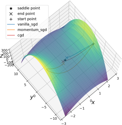
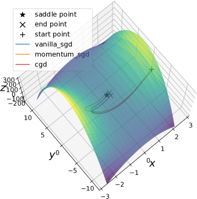
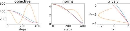
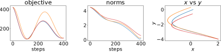
As an objective function, we chose , which matches the experimental setting of [Heu+17]. Here, is minimized with the derivative as the gradient direction and is maximized with the derivative as the gradient direction. With as the objective function, the LNE is .
The trajectory of optimization is shown in Figure 1 for a constant learning rate and diminishing learning rate with 0.5. This toy example confirms convergence to a LNE for an appropriate learning rate. We can see that each optimizer follows a different trajectory, but eventually reaches the same convergence point. The objective oscillates, but converges to (the value of the objective at LNE), and the norm decreases almost monotonically.
4.3 Experiments on GANs
We conducted a series of experiments using SNGAN with ResNet generator [Zhu+20]. To meet Assumption 2.1(A2), we replaced the batch normalization layer with a spectral normalization (SN) layer [Miy+18].
Here, we show that assumptions in Theorems 3.1 and 3.2 hold in the experiments. We used an SN layer to guarantee that (A2) holds (see also the above paragraph). We set , , , and to satisfy (C1), (C2), (D2), and (D3) before implementing Algorithm 1. The experiments indicated the boundedness (C3) of and . To guarantee that Algorithm 1 satisfies (C3) before implementing the algorithm, we replaced and in Algorithm 1 with and , where and are projections onto closed balls with sufficiently large radii. A discussion similar to the one proving Theorems 3.1 and 3.2, together with the nonexpansivity condition of the projection (), leads to versions of Theorems 3.1 and 3.2 for all and belonging to the closed balls. Meanwhile, it would be difficult to check whether (D1) holds in practical GANs. However, even if (D1) does not hold, Theorems 3.1 and 3.2(ii) are guaranteed to hold.
In this experimental setting, the loss function is high-dimensional and non-convex, so a simple gradient norm does not necessarily correspond to the quality of learning of the GANs. Here, the Fréchet inception distance (FID) [Heu+17] is commonly used to evaluate the quality of GAN training, so we chose it as a metric to evaluate the training on real-world data. The smaller the value of this metric is, the better the training of the generator of the GANs becomes. For the CG methods, we tested the seven beta update rules described in Section 2.2.
For the hyperparameter search, we conducted a grid search for all optimizers and datasets. The details of the hyperparameters are in Appendix D.3, and the remaining experimental settings are detailed in Appendix D.
4.3.1 Constant learning rate rule
A constant learning rate is practically used for training GANs, including those in [Heu+17], [Zhu+20]. Before conducting the diminishing learning rate experiment, we compared the training behaviors of the four optimizers when using a constant learning rate. We focused on the optimization methods shown in Table 1. Still, for real-world problems, it is desirable to consider cases in which a popular optimizer such as Adam is used. Therefore, we compared SGD, Momentum SGD, Adam, and seven CG algorithms when SNGAN with ResNet generator is used as the model on the CIFAR10 dataset.
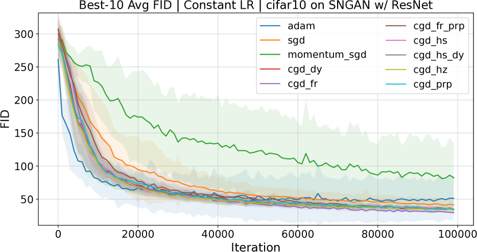
Comparing the FID scores of the trained model by the CG method and the other optimizers in Table 3 reveals that the CG methods outperformed the conventional optimizers (SGD and momentum SGD) in the case of the constant learning rate schedule.
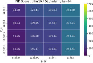
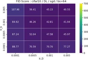
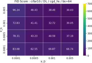
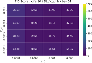
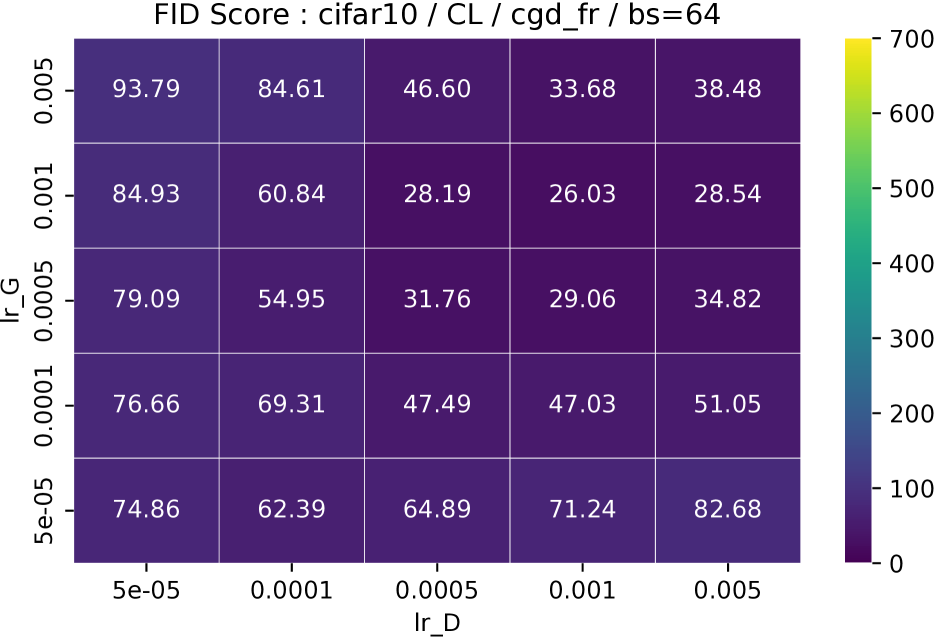
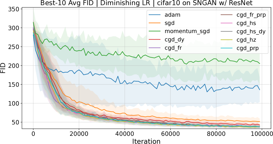
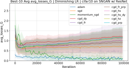
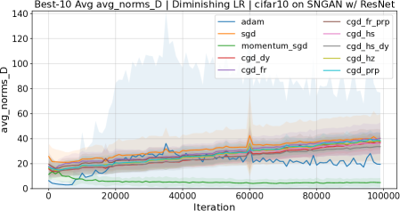
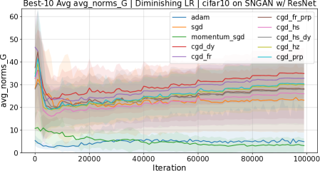
The experimental results showed that not only did the CG method outperform the other optimizers (including Adam) on average in terms of FID score in the best ten trials (Figure 2 Left), but it was also more robust than any other optimizer in terms of hyperparameter sensitivities (Figure 2 Right) (Details are in Appendix F).
4.3.2 Diminishing learning rate rule
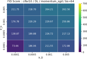
Here, we present experimental results in the case of a diminishing learning rate. To avoid learning stagnation due to an excessively decaying learning rate, we implemented the methods using LR with an initial LR and a rate that decays every iterations, where , , K, and .
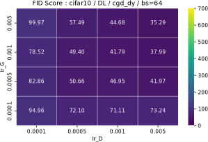
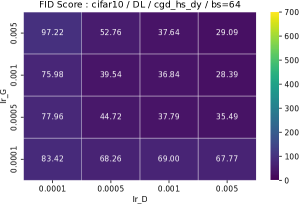
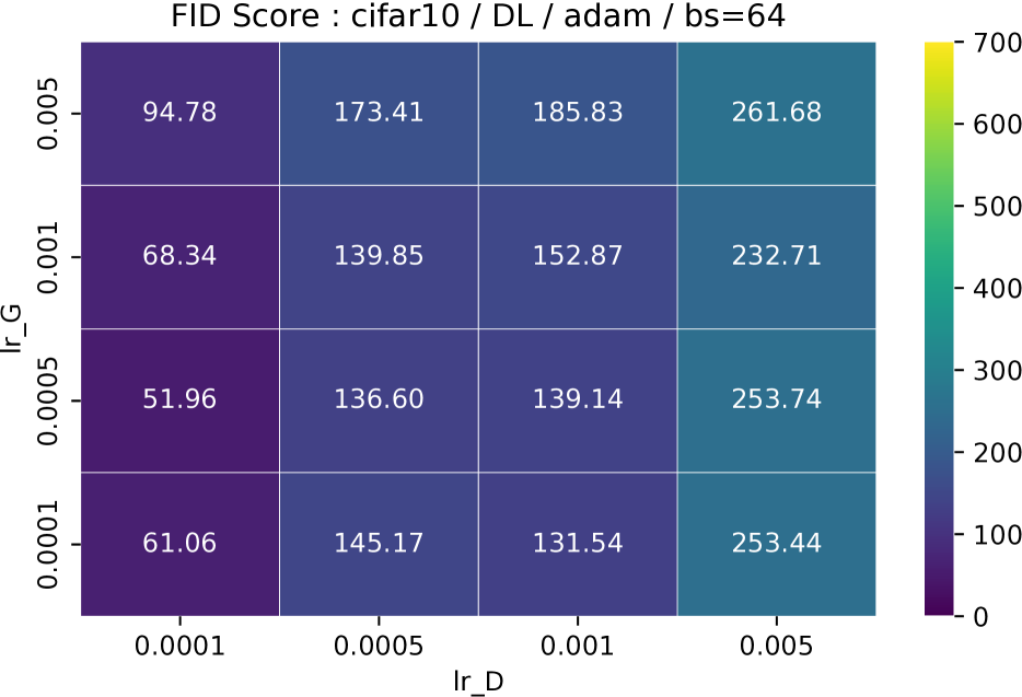
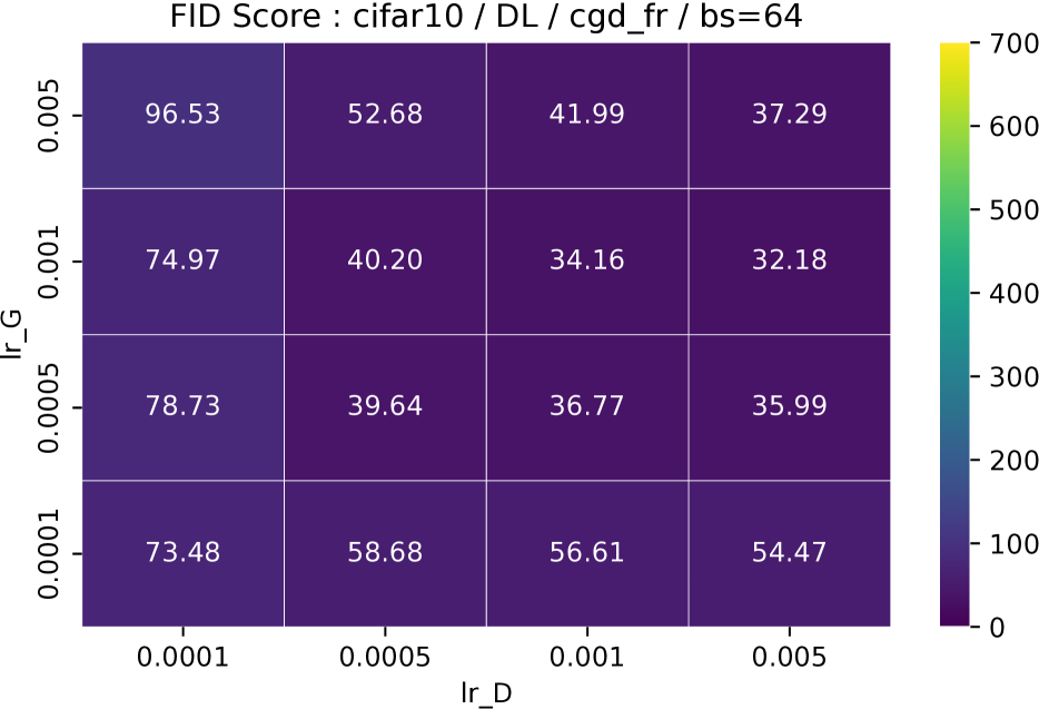
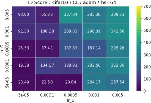
As can be seen from Table 3, the CG method achieved a competitive FID score close to that with a constant learning rate. In contrast, methods such as SGD, Momentum SGD, and Adam showed degraded performance. It should be noted that Adam can also achieve a reasonably good FID score by carefully tuning the hyperparameters, as shown in Figure 3 (Right). In contrast, the CG method is less sensitive to hyperparameters in the range of our experiments. The details of the other optimizers and results for other beta update rules for the CG method are shown in Appendix F.
5 Conclusion
For training GANs, we proposed CG-type algorithms to solve LNE problems and proved their convergence to LNEs under constant and diminishing learning rates under mild assumptions. Furthermore, we analyzed the convergence rates of the SGD, momentum SGD, and CG methods. We compared our method with SGD and momentum SGD on a toy problem, with experimental results consistent with theory. Finally, we evaluated the optimizer by training GANs using the FID score as a metric. We demonstrated that under constant and diminishing learning rates, the CG method outperformed SGD and momentum SGD and outperformed Adam on average in real-world problem settings.
One limitation of this study is that it involved experiments on only CIFAR10 datasets. Although the CG method minimized the FID scores in both cases, validations on other real-world datasets will be needed to support our claims. Another issue is that we did not use the state-of-the-art GAN model. We used a simple model to validate the theoretical contribution in Table 1 under corresponding conditions. Thus, our method still needs to be compared with, e.g., StyleGAN [KLA19] and other models that have shown high performance in recent years.
6 Acknowledgements
We are sincerely grateful to the meta-reviewer and the five anonymous reviewers for helping us improve the original manuscript. We would like to thank Charles Guille-Escuret (Mila, UdeM) and Reyhane Askari (Mila, UdeM) for their helpful feedback and also thank Tetsuya Motokawa (Tsukuba University) and Izumu Hosoi (University of Tokyo) for their help on the PyTorch implementation. This work was supported by the Masason Foundation Fellowship awarded to Hiroki Naganuma and by the Japan Society for the Promotion of Science (JSPS) KAKENHI Grant Number 21K11773 awarded to Hideaki Iiduka. This research used the computational resources of the TSUBAME3.0 supercomputer555https://www.t3.gsic.titech.ac.jp/en provided by Tokyo Institute of Technology through the Exploratory Joint Research Project Support Program from JHPCN (EX22401) and TSUBAME Encouragement Program for Young / Female Users.
References
- [Nas51] John Nash “Non-Cooperative Games” In Annals of Mathematics 54.2 Annals of Mathematics, 1951, pp. 286–295 URL: http://www.jstor.org/stable/1969529
- [HS52] M. Hestenes and E. Stiefel “Methods of conjugate gradients for solving linear systems” In Journal of research of the National Bureau of Standards 49, 1952, pp. 409–435
- [FR64] R. Fletcher and C.. Reeves “Function minimization by conjugate gradients” In The Computer Journal 7.2, 1964, pp. 149–154
- [Pol64] B.. Polyak “Some methods of speeding up the convergence of iteration methods” In USSR Computational Mathematics and Mathematical Physics 4, 1964, pp. 1–17
- [PR69] E. Polak and G. Ribiere “Note sur la convergence de méthodes de directions conjuguées” In ESAIM: Mathematical Modelling and Numerical Analysis - Modélisation Mathématique et Analyse Numérique 3.R1 Paris: Dunod, 1969, pp. 35–43 URL: http://www.numdam.org/item/M2AN_1969__3_1_35_0/
- [Pol69] B.T. Polyak “The conjugate gradient method in extremal problems” In USSR Computational Mathematics and Mathematical Physics 9.4, 1969, pp. 94–112 DOI: https://doi.org/10.1016/0041-5553(69)90035-4
- [HS91] Y. Hu and C. Storey “Global convergence result for conjugate gradient methods” In Journal of Optimization Theory and Applications 72, 1991, pp. 399–405
- [Møl93] Martin Fodslette Møller “A scaled conjugate gradient algorithm for fast supervised learning” In Neural Networks 6.4, 1993, pp. 525–533 DOI: https://doi.org/10.1016/S0893-6080(05)80056-5
- [Bor97] Vivek S. Borkar “Stochastic approximation with two time scales” In Systems & Control Letters 29.5, 1997, pp. 291–294 DOI: https://doi.org/10.1016/S0167-6911(97)90015-3
- [DY99] Y.. Dai and Y. Yuan “A Nonlinear Conjugate Gradient Method with a Strong Global Convergence Property” In SIAM Journal on Optimization 10.1, 1999, pp. 177–182 DOI: 10.1137/S1052623497318992
- [DY01] Y.. Dai and Y. Yuan “An Efficient Hybrid Conjugate Gradient Method for Unconstrained Optimization” In Annals of Operations Research 103, 2001, pp. 33–47
- [HZ05] W.. Hager and H. Zhang “A New Conjugate Gradient Method with Guaranteed Descent and an Efficient Line Search” In SIAM Journal on Optimization 16.1, 2005, pp. 170–192
- [HZ06] W.. Hager and H. Zhang “A survey of nonlinear conjugate gradient methods” In Pacific Journal of Optimization 2.1, 2006, pp. 35–58
- [NW06] Jorge Nocedal and Stephen J. Wright “Numerical Optimization” New York, NY, USA: Springer, 2006
- [Bor08] Vivek S. Borkar “Stochastic Approximation: A Dynamical Systems Viewpoint” Hindustan Book Agency: Springer, 2008
- [Le+11] Quoc V Le et al. “On optimization methods for deep learning” In ICML, 2011
- [Sut+13] I. Sutskever, J. Martens, G.. Dahl and G.. Hinton “On the importance of initialization and momentum in deep learning” In International Conference on Machine Learning, 2013, pp. 1139–1147
- [Goo+14] Ian Goodfellow et al. “Generative adversarial nets” In Advances in neural information processing systems 27, 2014
- [KB15] Diederik P. Kingma and Jimmy Ba “Adam: A Method for Stochastic Optimization” In 3rd International Conference on Learning Representations, ICLR 2015, San Diego, CA, USA, May 7-9, 2015, Conference Track Proceedings, 2015 URL: http://arxiv.org/abs/1412.6980
- [Mey+15] Simone Meyer et al. “Phase-based frame interpolation for video” In Proceedings of the IEEE conference on computer vision and pattern recognition, 2015, pp. 1410–1418
- [RMC15] Alec Radford, Luke Metz and Soumith Chintala “Unsupervised representation learning with deep convolutional generative adversarial networks” In arXiv preprint arXiv:1511.06434, 2015
- [Pat+16] Deepak Pathak et al. “Context encoders: Feature learning by inpainting” In Proceedings of the IEEE conference on computer vision and pattern recognition, 2016, pp. 2536–2544
- [Goo17] Ian J. Goodfellow “NIPS 2016 Tutorial: Generative Adversarial Networks” In CoRR abs/1701.00160, 2017 arXiv: http://arxiv.org/abs/1701.00160
- [Heu+17] M. Heusel et al. “GANs Trained by a Two Time-Scale Update Rule Converge to a Local Nash Equilibrium” In International Conference on Neural Information Processing Systems, 2017, pp. 1–12
- [Zha+17] Han Zhang et al. “Stackgan: Text to photo-realistic image synthesis with stacked generative adversarial networks” In Proceedings of the IEEE international conference on computer vision, 2017, pp. 5907–5915
- [Zhu+17] Jun-Yan Zhu, Taesung Park, Phillip Isola and Alexei A Efros “Unpaired image-to-image translation using cycle-consistent adversarial networks” In Proceedings of the IEEE international conference on computer vision, 2017, pp. 2223–2232
- [BDS18] Andrew Brock, Jeff Donahue and Karen Simonyan “Large scale GAN training for high fidelity natural image synthesis” In arXiv preprint arXiv:1809.11096, 2018
- [DMP18] Chris Donahue, Julian McAuley and Miller Puckette “Adversarial audio synthesis” In arXiv preprint arXiv:1802.04208, 2018
- [FGD18] William Fedus, Ian Goodfellow and Andrew M Dai “Maskgan: better text generation via filling in the_” In arXiv preprint arXiv:1801.07736, 2018
- [Miy+18] Takeru Miyato, Toshiki Kataoka, Masanori Koyama and Yuichi Yoshida “Spectral Normalization for Generative Adversarial Networks” In CoRR abs/1802.05957, 2018 arXiv: http://arxiv.org/abs/1802.05957
- [RKK18] Sashank J. Reddi, Satyen Kale and Sanjiv Kumar “On the Convergence of Adam and Beyond” In 6th International Conference on Learning Representations, ICLR 2018, Vancouver, BC, Canada, April 30 - May 3, 2018, Conference Track Proceedings OpenReview.net, 2018 URL: https://openreview.net/forum?id=ryQu7f-RZ
- [Gid+19] Gauthier Gidel et al. “Negative momentum for improved game dynamics” In The 22nd International Conference on Artificial Intelligence and Statistics, 2019, pp. 1802–1811 PMLR
- [HAU19] Hideaki Hayashi, Kohtaro Abe and Seiichi Uchida “GlyphGAN: Style-consistent font generation based on generative adversarial networks” In Knowledge-Based Systems 186 Elsevier, 2019, pp. 104927
- [Hon+19] Yongjun Hong, Uiwon Hwang, Jaeyoon Yoo and Sungroh Yoon “How generative adversarial networks and their variants work: An overview” In ACM Computing Surveys (CSUR) 52.1 ACM New York, NY, USA, 2019, pp. 1–43
- [KLA19] Tero Karras, Samuli Laine and Timo Aila “A style-based generator architecture for generative adversarial networks” In Proceedings of the IEEE/CVF conference on computer vision and pattern recognition, 2019, pp. 4401–4410
- [San+19] Veit Sandfort, Ke Yan, Perry J Pickhardt and Ronald M Summers “Data augmentation using generative adversarial networks (CycleGAN) to improve generalizability in CT segmentation tasks” In Scientific reports 9.1 Nature Publishing Group, 2019, pp. 1–9
- [Zhu+20] Juntang Zhuang et al. “AdaBelief Optimizer: Adapting Stepsizes by the Belief in Observed Gradients” In Advances in Neural Information Processing Systems 33: Annual Conference on Neural Information Processing Systems 2020, NeurIPS 2020, December 6-12, 2020, virtual, 2020 URL: https://proceedings.neurips.cc/paper/2020/hash/d9d4f495e875a2e075a1a4a6e1b9770f-Abstract.html
- [Sun+21] Tao Sun et al. “Training Deep Neural Networks with Adaptive Momentum Inspired by the Quadratic Optimization” In arXiv preprint arXiv:2110.09057, 2021
Appendix A Lemmas
We define and . We prove the following lemma:
Lemma A.1
Under (A1), (A2), and (C3), for all ,
where and denote upper bounds of and for all and all , respectively. Additionally, under (C2), we have that, for all ,
where .
Proof of Lemma A.1: Let be fixed arbitrarily. Assumption (C3) implies that there exists such that . Assumption (A2) thus implies that, for all ,
Assumption (A1) ensures that is continuous. Hence, (C3) guarantees that there exists such that . The triangle inequality guarantees that, for all ,
which implies that
Accordingly,
Let us define . We will use mathematical induction to show that, for all , . When , we have that
where the second inequality comes from the condition . Assume that for some . We have that
Hence, we have that, for all , .
A discussion similar to the one proving Lemma A.1 leads to the following.
Lemma A.2
Under (A1), (A2), and (C3), for all ,
where and denote upper bounds of and for all and all , respectively. Additionally, under (C2), we have that, for all ,
where .
Lemma A.3
Under the assumptions in Lemma A.1, for all , all , and all ,
Proof of Lemma A.3: Let and be fixed arbitrarily. The definition of ensures that
which, together with the Cauchy–Schwarz inequality and Lemma A.1, implies that
Accordingly, Lemma A.1 and Jensen’s inequality give
From the definition of , we also have that
Let us denote the independent and identically distributed samples considered here by and denote the history of process to time step by . Accordingly, we have
Therefore, we have
The definition of guarantees that
Taking the expectation of the above inequality gives
A discussion similar to the one showing the above inequality leads to the following inequality:
This completes the proof.
Appendix B Proofs of Theorems 3.1 and 3.2
B.1 Outline of Theorem 3.1
First, we provide a brief outline of the proof. Assumptions 2.1(A1)–(A2) and 3.1(C2)–(C3) imply that and are bounded (Lemmas A.1 and A.2). Next, we evaluate the squared norm () to find the relationship between and . Using the expansion of the squared norm leads to
The definition of and the boundedness of imply that there exist positive constants and , which depend on (A2) and (C3), such that, for all ,
| (16) |
Inequality (16) is a key inequality to prove Theorem 3.1. We can show (6) by contradiction and (16) with (C1). The limit inferior of in (6) ensures that there exists a subsequence of such that converges almost surely to satisfying that, for all ,
which, together with , implies that
Accordingly, we have (7). A discussion similar to the one showing (16) leads to the following key inequality: there exist positive constants and , which depend on (A2) and (C3), such that, for all ,
| (17) |
A discussion similar to the one showing (6) and (7), together with (17), leads to (8) and (9). Summing (16) with (C1) from to gives (LABEL:sum_g). Similarly, summing (17) from to gives (LABEL:sum_d). Let us consider the case where converges almost surely to . Inequalities (7) and (9) thus guarantee (12).
The following is the detailed proof of Theorem 3.1.
Proof of Theorem 3.1: Let and be fixed arbitrarily. First, we show that, for all ,
| (18) |
If (18) does not hold, then there exists such that
Since there exists such that, for all ,
we have that, for all ,
Lemma A.3, together with (C1) and (C2), ensures that, for all ,
| (19) |
Accordingly, for all ,
approaches minus infinity as approaches positive infinity. This is a contradiction. Hence, (18) holds. Since is arbitrary, we have that
| (20) |
A discussion similar to the one showing the above inequality leads to the following:
| (21) |
Inequality (20) ensures that there exists a subsequence of such that, for all ,
Assumption (C3) implies that there exists of such that converges almost surely to . Accordingly, for all ,
which implies that
| (22) |
A discussion similar to the one showing the above inequality, together with (21), means that there exists a subsequence of such that converges almost surely to satisfying
| (23) |
Inequality (19) implies that
Summing the above inequality from to guarantees that
which implies that
| (24) |
A discussion similar to the one showing (24) leads to the following:
Let us consider the case where converges almost surely to . Inequalities (22) and (23) indicate that
which completes the proof.
B.2 Proof outline of Theorem 3.2
First, we provide a brief outline of the proof. The flow is the same as in [Bor97]. The definitions of and imply that, for all ,
| (25) | ||||
We can easily check that (25) is as a discretized version of the ordinary differential equations and with a step size and errors at the th iteration defined by
| (26) |
Assumptions 3.1(C2) and 3.2(D2)(i) thus guarantee that two sequences defined by (26) converge almost surely to zero. Hence, an argument similar to the one for obtaining Theorem 1.1 in [Bor97] (see [Bor97, Section 2] for the detailed proof) leads to Theorem 3.2(i). Theorem 3.2(ii) depends on the key inequalities (16) and (17), which come from Assumptions 2.1(A1)–(A2) and 3.1(C2)–(C3). Summing (16) and (17) from to gives (13). In particular, let us define , , , and , where . These learning rates satisfy Assumption 3.2(D2)(ii) and (D3). Hence, (13) implies (14). Moreover, we use and defined by (15). These learning rates satisfy Assumption 3.2(D2)(ii) and (D3). Hence, (13) implies (14).
The following is the detailed proof of Theorem 3.2.
Proof of Theorem 3.2: (i) The definitions of and imply that, for all ,
| (27) | ||||
Lemma A.1 ensures that , , , and are almost surely bounded. Assumption 3.2(D1) ensures that (27) can be regarded as a discretized version of the ordinary differential equations and with a step size and errors at the -th iteration defined by
| (28) |
Assumptions 3.1(C2) and 3.2(D2)(i) thus guarantee that two sequences defined by (28) converge almost surely to zero. Hence, an argument similar to the one proving Theorem 1.1 in [Bor97] (see [Bor97, Section 2] for the details of the proof) leads to Theorem 3.2(i).
(ii) Lemma A.3 guarantees that, for all and all ,
Summing the above inequality from to gives, for all ,
We have that
Since is monotone decreasing, we have that, for all , . Moreover, for all , . Hence,
Therefore, for all and all ,
A discussion similar to the one showing the above inequality leads to the following: for all and all ,
Let us define , where . Then, we have
and
Theorem 3.2(ii) thus leads to
where and .
Let us define
where , , and . Let and such that . Then, we have
When satisfies , Theorem 3.2(ii) leads to
This completes the proof.
Appendix C Examples of Algorithm 1
C.1 Examples of Algorithm 1 with constant learning rates
Properties (LABEL:sum_g), (LABEL:sum_d), and (12) in Theorem 3.1 indicate that, for sufficiently small learning rates and and CG parameters and ,
with
| (29) | ||||
Let us discuss the results in Theorem 3.1 under certain conditions. For simplicity, we assume that generated by Algorithm 1 converges almost surely to .
(I) [SGD] First, we consider the case where . In this case, Algorithm 1 for the generator (resp. the discriminator) is based on the SGD method with a learning rate (resp. ). Theorem 3.1 indicates that the convergent point of the SGD-type algorithm satisfies
(II) [Momentum SGD] We consider the case where and . In this case, Algorithm 1 for the generator (resp. the discriminator) is based on the momentum method with a learning rate (resp. ) and momentum coefficient (resp. ). Theorem 3.1 indicates that the convergent point of the momentum-type algorithm satisfies
| (30) |
(III) [CG] We consider the case where and are based on the CG formulas defined in Section 2.2. The parameters and satisfying (C2) are, for example, as follows:
| (31) |
where , , and .
| (32) |
where , , and . Theorem 3.1 indicates that the convergent point of the CG-type algorithm with and defined by (31) and (32) satisfies (30).
C.2 Examples of Algorithm 1 with diminishing learning rates
Property (14) together with666The maximum value of for is when .
| (33) |
indicates that Algorithm 1 satisfies
| (34) |
where we assume that the stochastic gradient errors and are zero. To guarantee that Algorithm 1 converges almost surely to a stationary Nash equilibrium, we need to set diminishing learning rates and satisfying Assumption 3.2(D2)(i), i.e.,
| (35) |
(see Theorem 3.2(i)). Then, property (14) ensures that Algorithm 1 has the following convergence rate:
| (36) |
where and .
Let us discuss the results in Theorem 3.2 under certain conditions.
(I) [SGD] First, we consider the case where . In this case, Algorithm 1 for the generator (resp. the discriminator) is based on the SGD method with a learning rate (resp. ). This algorithm was presented in [Heu+17, (1)]. Theorem 3.2(ii) indicates that the SGD-type algorithm satisfies (34) and (36); i.e.,
(II) [Momentum SGD] Let us consider Algorithm 1 for the generator (resp. the discriminator) based on the momentum method with a learning rate (resp. ) and momentum coefficient (resp. ). Let us consider and with (35). Then, there exists such that, for all , , which implies that and satisfy (C2). Theorem 3.2(ii) thus ensures that the momentum-type algorithm has the same convergence rate as in (I).
(III) [CG] Let us consider the CG-type algorithm, i.e., Algorithm 1 with and with (33) and and defined by (31) and (32). Theorem 3.2(i) guarantees that the CG-type algorithm converges almost surely to a point in . Next, let us consider and defined as follows:
| (37) |
where , , and .
| (38) |
where , , and . The sequences and defined by (37) and (38) satisfy (C2) and (D4). Property (14) ensures that the CG-type algorithm has the the same convergence rate as in (I).
Appendix D Experimental Settings
D.1 Implementation and environment
We performed our experiment on TSUBAME, a supercomputer owned by the Tokyo Institute of Technology. The total computation amounted to 65,900 GPU hours.
The dataset of CIFAR10777https://www.cs.toronto.edu/ kriz/cifar.html does not indicate a license. The pre-trained model is under Apache License 2.0 for the FID inception weights888https://github.com/mseitzer/pytorch-fid/releases.
Our code can be found at the link below.
https://github.com/Hiroki11x/ConjugateGradient_GAN
D.2 Model and datasets
We studied and evaluated SNGAN with ResNet generator [Zhu+20] for GAN experiments. We used CIFAR10 as the dataset. The workload for each experimental setup is shown in Table 4.
| Model | Dataset | Dataset Size | Step Budget |
|---|---|---|---|
| SNGAN with ResNet Generator [Zhu+20] | CIFAR10 | 50000 | 100K |
D.3 Hyperparameters and detailed configuration
D.3.1 Toy-example experiments
The hyperparameters for the results shown in Figure 1 of Section 4.2 are explained here. A momentum coefficient of 0.9 was used for momentum SGD, and FR was set as a beta update for the CG method. Each optimizer had a learning rate to update x and a learning rate to update y. For the constant learning rate settings, we set as the learning rate of x and as the learning rate of y in SGD. Moreover, we set and in the momentum SGD and and in the CG method. The number of steps was 400. After updating x, the gradient of y was updated for the objective function, which used the updated x.
D.3.2 GAN experiments
Here, we report the hyperparameter’s search space. For SGD, we only searched the learning rate and batch size . For momentum SGD, was added a fixed value of 0.9 as a parameter to control the momentum . As for the diminishing learning rates, we performed experiments as described in Section 4.3.2.
| Optimizer | Update Rule | 111: Initial learning rate for generator (Learning rate for Generator) | 222: Initial learning rate for discriminator (Learning rate for Discriminator) | Learning rate Scheduler Type | ||||
|---|---|---|---|---|---|---|---|---|
| SGD | - | {64} |
|
|
|
|||
| Momentum SGD | - | {64} |
|
|
|
|||
| Adam | - | {64} |
|
|
|
|||
| CG | FR | {64} |
|
|
|
|||
| CG | PRP | {64} |
|
|
|
|||
| CG | HS | {64} |
|
|
|
|||
| CG | DY | {64} |
|
|
|
|||
| CG | HZ | {64} |
|
|
|
|||
| CG | Hyb1 (HS, DY) | {64} |
|
|
|
|||
| CG | Hyb2 (FR, PRP) | {64} |
|
|
|
Appendix E Supplemental Experimental Results
This section provides information on experimental results omitted from the text.
Adam, a popular optimizer in the training of GANs, was compared. Here, when Adam is used to train GANs, it has been reported that setting , the hyperparameter of Adam’s first order moment, to 0.5 leads to stable learning [RMC15], and it was used in [Heu+17]’s work. Therefore, we chose this setting.
E.0.1 Constant learning rate rule
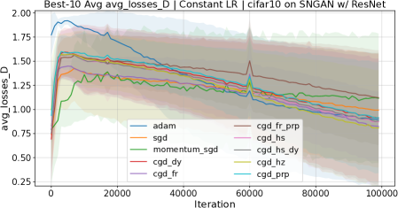
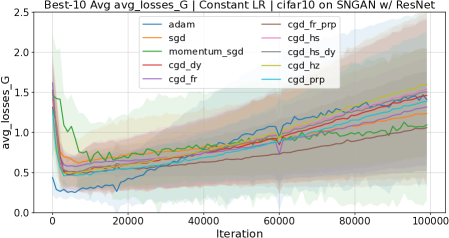
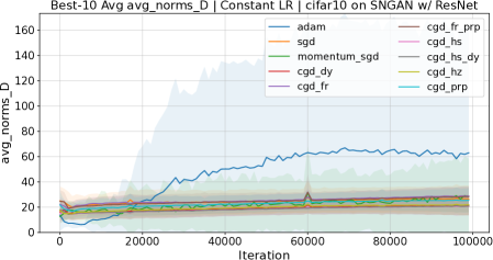
In the case of a constant learning rate, the discriminator’s loss decreased steadily, increasing the generator’s loss (Figure 5). The CG method using FR as a update rule had the best FID score: the discriminator’s loss decreased steadily, and the generator’s loss increased, suggesting convergence to the saddle point. The norm transition for the gradient is shown in Figure 6. The FID transition is shown in Figure 4, and the final scores are shown in Table 3.
Additionally, the details of the FID scores for each learning-rate combination are shown in Figure 10 in Appendix F.


E.0.2 Diminishing learning rate rule
The inverse square learning rate was not used in the previous studies [Heu+17, Goo17, RMC15] because of the rapid decay of the learning rate from the beginning to the middle of the learning process, which is challenging to balance in minimax optimization. Therefore, we employed a scheduling scheme that decays the learning rate every steps.
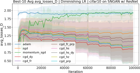
The details of the FID scores for each learning-rate combination are shown in Figures 11 in Appendix F. The FID scores for training with the diminishing learning rate are shown in Figure 7. The losses and norms of each generator and discriminator for training on the MNIST and CIFAR10 are shown in Figure 8 and Figure 9, respectively.

Appendix F Sensitivity of learning rate
F.1 Constant learning rate rule
For the dataset optimizer combinations, we performed a grid search of 25 hyperparameter combinations, including five combinations each for LR_G (initial learning rate for the generator) and LR_D (initial learning rate for the discriminator). To evaluate the optimizer’s performance on LR_G and LR_D, we created a heat map of FID scores.
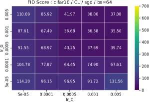
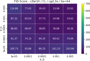
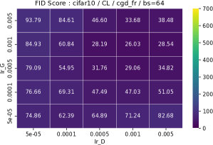
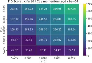
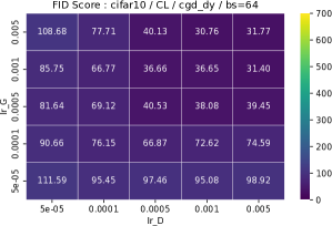


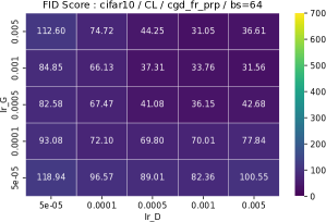
F.2 Diminishing learning rate rule
For dataset optimizer combinations, we performed a grid search of 16 hyperparameter combinations, including five combinations each for LR_G (initial learning rate for generator) and LR_D (initial learning rate for discriminator). To evaluate the optimizer’s performance on LR_G and LR_D, we created a heat map of FID scores.