A nonlocal Stokes system with volume constraints

Abstract

In this paper, we introduce a nonlocal model for linear steady Stokes system with physical no-slip boundary condition. We use the idea of volume constraint to enforce the no-slip boundary condition and prove that the nonlocal model is well-posed. We also show that and the solution of the nonlocal system converges to the solution of the original Stokes system as the nonlocality vanishes.

1 Introduction

Recently, nonlocal models and corresponding numerical methods have attracted much attention due to many successful applications. For example, in solid mechanics, the theory of peridynamics [38] has been used as a possible alternative to conventional models of elasticity and fracture mechanics. Many numerical methods have also been developed to simulate nonlocal models like peridynamics based on rigorous mathematical analysis [10, 30, 31, 39, 12, 11, 43]. Nonlocal methods are also successfully applied in image processing and data analysis [34, 33, 2, 6, 23, 20, 35, 19, 22, 4, 29, 41]. The idea of integral approximation is also applied to derive numerical scheme for solving PDEs on point cloud [25, 26].

In this paper, we study the nonlocal analog of the Stokes system in fluid mechanics. Previously, nonlocal Stokes models have been proposed in [13] and [24] and analyzed subject to periodic boundary condition. In this paper, we consider the case of a nonlocal no-slip boundary condition. More precisely, for the conventional, local linear Stokes system on a domain $\Omega\subset\mathbb{R}^{n}$,

(1.3) $$\left\{\begin{array}[]{rcl}\Delta{\bm{u}}(\bm{x})-\nabla p(\bm{x})&=&{\bm{f}}(\bm{x}),\quad\bm{x}\in\Omega\\ \nabla\cdot{\bm{u}}(\bm{x})&=&0,\quad\bm{x}\in\Omega,\end{array}\right.,$$

the no-slip boundary condition on the boundary $\partial\Omega$ is

(1.4) $${\bm{u}}=0,\quad\quad\text{at}\;\;\partial\Omega.$$

For the pressure, we impose average zero condition

(1.5) $$\int_{\Omega}p(\bm{x})\mathrm{d}\bm{x}=0.$$

The no-slip boundary condition is a Dirichlet type boundary condition and it is often used in many real world applications. However, the theoretical study with no-slip boundary condition is also much more difficult. The first question is how to enforce no-slip boundary condition in the nonlocal approach. Recently, Du et.al. [10] proposed volume constraint to deal with the boundary condition in the nonlocal diffusion problem by enforcing the condition over a nonlocal region adjacent to the boundary. Adopting this idea, in the nonlocal Stokes system, we extend the no-slip condition to a small layer as shown in Fig. 1.

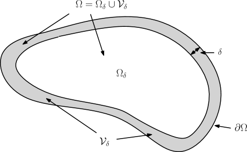
Fig. 1: Computational domain in non-local Stokes model.

For a nonlocal problem involving nonlocal interactions on the range of $\delta>0$, the whole computational domain $\Omega$ is decomposed to two parts. $\Omega=\mathcal{V}_{\delta}\bigcup\Omega_{\delta}$ as shown in Fig. 1 and ${\bm{u}}$ is enforced to be zero in ${\mathcal{V}}_{\delta}$, i.e.

(1.6) $${\bm{u}}_{\delta}(\bm{x})=0,\quad\bm{x}\in\mathcal{V}_{\delta}.$$

Definition of $\Omega_{\delta}$ and $\mathcal{V}_{\delta}$ will be given in (2.1). The parameter $\delta$ is often called the nonlocal horizon parameter [38, 9]. In $\Omega_{\delta}$, the Stokes equation is approximated is formualted as

(1.9) $$\left\{\begin{array}[]{rclc}\displaystyle\mathcal{L}_{\delta}{\bm{u}}_{\delta}(\bm{x})-\displaystyle\mathcal{G}_{\delta}p_{\delta}(\bm{x})&=&{\displaystyle\int_{\Omega}\bar{R}_{\delta}(\bm{x},\bm{y}){\bm{f}}(\bm{y})\mathrm{d}\bm{y}},&\bm{x}\in\Omega_{\delta},\\ \displaystyle\mathcal{D}_{\delta}{\bm{u}}_{\delta}(\bm{x})-\bar{\mathcal{L}}_{\delta}p_{\delta}(\bm{x})&=&0,&\bm{x}\in\Omega.\\ \end{array}\right.$$

The nonlocal integral operators used in (1.9) represent the nonlocal diffusion (Laplacian) $\mathcal{L}_{\delta}$, nonlocal gradient $\mathcal{G}_{\delta}$ and nonlocal divergence $\mathcal{D}_{\delta}$ respectively as in [13] and the references cited therein. An additional operator $\bar{\mathcal{L}}_{\delta}$ is also used, which is a rescaled nonlocal diffusion operator. The particular forms of the operators adopted here are given by

(1.10) $$\mathcal{L}_{\delta}{\bm{u}}(\bm{x}) =\frac{1}{\delta^{2}}\int_{\Omega}R_{\delta}(\bm{x},\bm{y})({{\bm{u}}(\bm{y})-{\bm{u}}(\bm{x})})\mathrm{d}\bm{y},$$

(1.11) $$\mathcal{G}_{\delta}p(\bm{x}) =\frac{1}{2\delta^{2}}\int_{\Omega}R_{\delta}(\bm{x},\bm{y})({\bm{y}-\bm{x}})p(\bm{y})\mathrm{d}\bm{y},$$

(1.12) $$\mathcal{D}_{\delta}{\bm{u}}(\bm{x}) =\frac{1}{2\delta^{2}}\int_{\Omega}R_{\delta}(\bm{x},\bm{y})({\bm{y}-\bm{x}})\cdot{\bm{u}}(\bm{y})\mathrm{d}\bm{y},$$

(1.13) $$\bar{\mathcal{L}}_{\delta}p(\bm{x}) =\int_{\Omega}\bar{R}_{\delta}(\bm{x},\bm{y})({p(\bm{y})-p(\bm{x})})\mathrm{d}\bm{y},$$

for some nonnegative and smooth kernels $R_{\delta}(\bm{x},\bm{y})$ and $\bar{R}_{\delta}(\bm{x},\bm{y})$ specified later.

Finally, we also need average zero condition for the pressure

(1.14) $$\int_{\Omega}p_{\delta}(\bm{x})\mathrm{d}\bm{x}=0.$$

(1.6), (1.9) and (1.14) form a complete nonlocal formulation of the Stokes system.

As pointed out in the literature on nonlocal modeling (e.g. [13, 9]), nonlocal integral approximations are closely related to many numerical schemes of computational fluid dynamics, such as the smoothed particle hydrodynamics (SPH) [18, 27, 28, 32], vortex methods [1, 7] and others [3, 5, 15, 21, 40]. Analysis to the linear steady Stokes equation in this paper could give some new understanding to the theoretical foundation of these methods.

The Stokes system (1.3) is well-known to be a saddle point problem. This remains the case for the nonlocal Stokes system given in [13] subject to periodic boundary conditions. Here, different from [13], we add a relaxation term, $\bar{\mathcal{L}}_{\delta}p_{\delta}(\bm{x})$, in the second equation of (1.9). It mimics the classical technique of stabilizing the approximation of incompressibility by adding a positive definite block to the original saddle point system. Although this results in a slightly compressible system, the stabilization term vanishes as $\delta\to 0$ so that it does not destroy the approximation of the nonlocal formulation to the local limit. Yet, this additional term is crucial for the stability and well-posedness in our case where smooth nonlocal kernels are used to define the nonlocal operators. Indeed, the well-posed study in [13] showed that, without extra relaxation, it is necessary to use singular kernels. A remedy was provided in [24] by incorporating non-radial nonlocal interactions. The addition of the relaxation term enables the use of smooth kernels in the definition of the associated nonlocal operators which may allow more flexible practical implementation such as more conventional quadratures for smooth functions. For the Fourier analysis of a related formulation with periodic boundary conditions, we refer to [42].

The rest of the paper is organized as follows. We give the formulation of the nonlocal linear Stokes system in Section 2 together with some related assumptions and estimates. Then the well-posedness of the nonlocal model is established in Section 3. The vanishing nonlocality limit is analyzed in Section 4. In Section 5, we conclude with a summary and a discussion on future research.

2 Nonlocal Stokes system with related assumptions and estimates

In this section we present the nonlocal Stokes model in more details, together with some basic assumptions on the geometry and kernel functions used to define the model, along with some related estimates.

2.1 Notation and assumptions

First, we let $\Omega_{\delta}$ and $\mathcal{V}_{\delta}$ be subsets of $\Omega$ defined as

(2.1) $$\Omega_{\delta}=\left\{\bm{x}\in\Omega:B\left(\bm{x},2\delta\right)\cap\partial\Omega=\emptyset\right\},\quad\mathcal{V}_{\delta}=\Omega\backslash\Omega_{\delta}.$$

The relation of $\Omega$, $\partial\Omega$, $\Omega_{\delta}$ and $\mathcal{V}_{\delta}$ are showed in Fig. 1.

Next, we state the following assumptions on the domain $\Omega$ and a kernel function $R(r)$.

Assumption 1.

• Assumptions on the computational domain: ${\Omega}\in\mathbb{R}^{n}$ is open, bounded and connected. $\partial{\Omega}$ is $C^{2}$ smooth.

• Assumptions on the kernel function $R(r)$:

  • (regularity) $R\in C^{1}[0,1]$;

  • (positivity and compact support) $R(r)\geq 0$ and $R(r)=0$ for $\forall r>1$;

  • (nondegeneracy) $\exists\gamma_{0}>0$ so that $R(r)\geq\gamma_{0}$ for $0\leq r\leq\frac{1}{2}$.

Then, the rescaled kernels used in the definitions of the nonlocal operators are defined by

(2.2) $$R_{\delta}(\bm{x},\bm{y})=C_{\delta}R\left(\frac{\|\bm{x}-\bm{y}\|^{2}}{4\delta^{2}}\right),\quad\bar{R}_{\delta}(\bm{x},\bm{y})=C_{\delta}\bar{R}\left(\frac{\|\bm{x}-\bm{y}\|^{2}}{4\delta^{2}}\right){,}$$

where

(2.3) $$\bar{R}(r)=\int_{r}^{+\infty}R(s)\mathrm{d}s=\int_{r}^{1}R(s)\mathrm{d}s,$$

which satisfies obviously

$$\bar{R}^{\prime}(r)=\frac{d}{dr}\bar{R}(r)=R(r),\;\forall r\in\mathbb{R}^{+},\quad\text{and}\quad\bar{R}(r)=0,\;\forall r>1.$$

The constant $C_{\delta}=\alpha_{n}\delta^{-n}$ in (2.2) is a normalization factor so that

(2.4) $$\int_{\mathbb{R}^{n}}\bar{R}_{\delta}(\bm{x},\bm{y})\mathrm{d}\bm{y}=\alpha_{n}S_{n}\int_{0}^{1}\bar{R}(\frac{r^{2}}{4})r^{n-1}\mathrm{d}r=1$$

with $S_{n}$ denotes area of the unit sphere in $\mathbb{R}^{n}$. With this normalization factor, the local limits of $\mathcal{L}_{\delta}$, $\mathcal{G}_{\delta}$ and $\mathcal{D}_{\delta}$ recover the classical Laplacian $\Delta$, gradient and divergence operators respectively as $\delta$ goes to 0. Moreover, $\bar{\mathcal{L}}_{\delta}$ also behaves like a nonlocal analog of $\beta_{n}\delta^{2}\Delta$, that is, a scaled nonlocal Laplacian that vanishes in the local limit.

2.2 Nonlocal Stokes system with volume constraint

By combining the volume constraint boundary condition of ${\bm{u}}$ and the average zero condition of $p$, we have the nonlocal Stokes model given as follows:

(2.9) $$\left\{\begin{array}[]{rclc}\displaystyle\mathcal{L}_{\delta}{\bm{u}}_{\delta}(\bm{x})-\displaystyle\mathcal{G}_{\delta}p_{\delta}(\bm{x})&=&{\displaystyle\int_{\Omega}\bar{R}_{\delta}(\bm{x},\bm{y}){\bm{f}}(\bm{y})\mathrm{d}\bm{y}},&\bm{x}\in\Omega_{\delta},\\ \displaystyle\mathcal{D}_{\delta}{\bm{u}}_{\delta}(\bm{x})-\bar{\mathcal{L}}_{\delta}p_{\delta}(\bm{x})&=&0,&\bm{x}\in\Omega,\\[2.84544pt] {\bm{u}}_{\delta}(\bm{x})&=&0,&\bm{x}\in\mathcal{V}_{\delta},\\ \displaystyle\int_{\Omega}p_{\delta}(\bm{x})\mathrm{d}\bm{x}&=&0.\end{array}\right.$$

The integral operators have been defined in (1.10)-(1.13). A formal derivation of the nonlocal model is given in the appendix A.

Formally, the choices of normalization specified in this paper further imply that the local limits of $\mathcal{L}_{\delta}$, $\mathcal{G}_{\delta}$ and $\mathcal{D}_{\delta}$ recover the classical Laplacian $\Delta$, gradient and divergence operators respectively as $\delta$ goes to 0 [31, 9]. Moreover, $\bar{\mathcal{L}}_{\delta}$ also behaves like a nonlocal analog of $\beta_{n}\delta^{2}\Delta$, that is, a scaled nonlocal Laplacian that vanishes in the local limit. Thus, we may see (2.9) as a nonlocal extension of the local Stokes model (1.3)-(1.4).

Remark 2.1.

For the study of the nonlocal model with periodic boundary condition on $\Omega=(0,1)^{n}$, we can use Fourier transform to get the Fourier symbols of the nonlocal operators, see the discussion in [42].

2.3 Related estimates

Next, we list several technical results of the kernel functions which will be used in the subsequent analysis.

Lemma 1.

Let $R=R(r)$ be a kernel function satisfying Assumption 1 and $R_{\delta}$, $\bar{R}_{\delta}$ be given by (2.2) and (2.3) respectively. i) There exist a constant $C>0$, independent of $\delta$, such that

$$|\nabla_{\bm{x}}\bar{R}_{\delta}(\bm{x},\bm{y})|\leq\frac{C}{\delta}R_{\delta}(\bm{x},\bm{y}).$$

$$|\nabla_{\bm{y}}\nabla_{\bm{x}}\bar{R}_{\delta}(\bm{x},\bm{y})|\leq\frac{C}{\delta^{2}}\left(|R^{\prime}_{\delta}(\bm{x},\bm{y})|+|R_{\delta}(\bm{x},\bm{y})|\right),$$

for any $\bm{x},\bm{y}\in\mathbb{R}^{n}$, where $R^{\prime}_{\delta}(\bm{x},\bm{y})=C_{\delta}R^{\prime}\left(\frac{\|\bm{x}-\bm{y}\|^{2}}{4\delta^{2}}\right)$ and $R^{\prime}(r)=\frac{\mathrm{d}R(r)}{\mathrm{d}r}$;

ii) Let $\tilde{R}$ be a kernel function satisfying the Assumption 1 (a) (b) and $\tilde{R}_{\delta}(\bm{x},\bm{y})=\alpha_{n}\delta^{-n}\tilde{R}\left(\frac{\|\bm{x}-\bm{y}\|^{2}}{4\delta^{2}}\right)$. There exists a constant $\eta_{0}>0$ only dependent on $\Omega$ and $\tilde{R}$, such that for $\delta\leq\eta_{0}$

$$\frac{\tilde{\omega}_{n}}{3}<{\tilde{\omega}_{\delta}(\bm{x}):=}\int_{\Omega}\tilde{R}_{\delta}(\bm{x},\bm{y})\mathrm{d}\bm{y}\leq\tilde{\omega}_{n}:=\alpha_{n}S_{n}\int_{0}^{1}\tilde{R}(\frac{r^{2}}{4})r^{n-1}\mathrm{d}r,$$

iii) Let

$$K_{\delta}(\bm{y},\mathbf{z})=\int_{\Omega}|\tilde{R}_{\delta}(\bm{x},\mathbf{z})\nabla_{\bm{x}}\tilde{R}_{\delta}(\bm{x},\bm{y})|\mathrm{d}\bm{x}.$$

for any $\bm{y},\mathbf{z}\in\mathbb{R}^{n}$. There exist $C>0$ independent on $\delta$ such that

$$K_{\delta}(\bm{y},\mathbf{z})\leq C{R}\left(\frac{\|\bm{y}-\mathbf{z}\|^{2}}{32\delta^{2}}\right),$$

Proof.

i) can be checked directly.
ii). This estimate is classical for smooth mollifiers. For the sake of completeness, we give a brief proof here. The upper bound is easy to prove using the non-negativity of $\tilde{R}_{\delta}$.

$${\tilde{\omega}_{\delta}(\bm{x})=}\int_{\Omega}{\tilde{R}}_{\delta}(\bm{x},\bm{y})\mathrm{d}\bm{y}\leq\int_{\mathbb{R}^{n}}{\tilde{R}}_{\delta}(\bm{x},\bm{y})\mathrm{d}\bm{y}={\tilde{\omega}_{n}}$$

To prove the lower bound, we need to use the condition that $\partial\Omega$ is $C^{2}$ and $\tilde{R}_{\delta}$ is continuous and bounded. Then for $\bm{x}\in\partial\Omega$,

$${\lim_{\delta\rightarrow 0}\tilde{\omega}_{\delta}(\bm{x})=}\lim_{\delta\rightarrow 0}\int_{\Omega}{\tilde{R}}_{\delta}(\bm{x},\bm{y})\mathrm{d}\bm{y}={\alpha_{n}}\int_{{\bm{x}+}\mathbb{R}^{n}_{+}}{\tilde{R}\left(\frac{\|\bm{x}-\bm{y}\|^{2}}{4}\right)}\mathrm{d}\bm{y}=\frac{\tilde{\omega}_{n}}{2},$$

where $\mathbb{R}^{n}_{+}=\{\bm{y}=(y_{1},\cdots,y_{n})\in\mathbb{R}^{n}:y_{1}\geq 0\}$.

On the other hand, for $\bm{x}\in{\Omega}$, since $\Omega$ is open,

$${\lim_{\delta\rightarrow 0}\tilde{\omega}_{\delta}(\bm{x})=}\lim_{\delta\rightarrow 0}\int_{\Omega}{\tilde{R}}_{\delta}(\bm{x},\bm{y})\mathrm{d}\bm{y}={\alpha_{n}}\int_{\mathbb{R}^{n}}{\tilde{R}\left(\frac{\|\bm{x}-\bm{y}\|^{2}}{4}\right)}\mathrm{d}\bm{y}=\tilde{\omega}_{n}.$$

So, for any $\bm{x}\in\bar{\Omega}=\Omega\cup\partial\Omega$, there exist $\eta_{\bm{x}}>0$ such that for any $\delta\leq\eta_{\bm{x}}$, we have ${\tilde{\omega}_{\delta}(\bm{x})}>{\tilde{\omega}_{n}}/{3}$. Using the compactness of $\bar{\Omega}$, there exists $\eta_{0}>0$ such that for any $\bm{x}\in\bar{\Omega}$, $\delta\leq\eta_{0}$, we have ${\tilde{\omega}_{\delta}(\bm{x})}>{\tilde{\omega}_{n}}/{3}$.

ii) When $\|\bm{y}-\mathbf{z}\|\geq 4\delta$, we have $\max\{\|\bm{x}-\mathbf{z}\|,\|\bm{x}-\bm{y}\|\}\geq 2\delta$, then using condition (a) and (b) in Assumption 1,

$$\tilde{R}_{\delta}(\bm{x},\mathbf{z})\nabla_{\bm{x}}\tilde{R}_{\delta}(\bm{x},\bm{y})=0,\quad\forall\bm{x}\in\Omega.$$

This gives that

$$K_{\delta}(\bm{y},\mathbf{z})=0,\quad\forall\|\bm{y}-\mathbf{z}\|\geq 4\delta.$$

When $\|\bm{y}-\mathbf{z}\|<4\delta$, we have $\frac{\|\bm{y}-\mathbf{z}\|^{2}}{32\delta^{2}}<\frac{1}{2}$. Using condition (c) in Assumption 1,

$$K_{\delta}(\bm{y},\mathbf{z})= \int_{\Omega}|\tilde{R}_{\delta}(\bm{x},\mathbf{z})\nabla_{\bm{x}}\tilde{R}_{\delta}(\bm{x},\bm{y})|\mathrm{d}\bm{x}$$

$$\leq \frac{1}{4\delta^{2}}\int_{\Omega}\|\bm{x}-\bm{y}\||\tilde{R}_{\delta}(\bm{x},\mathbf{z})||\tilde{R}^{\prime}_{\delta}(\bm{x},\bm{y})|\mathrm{d}\bm{x}$$

$$\leq \frac{1}{2\delta}\int_{\Omega}|\tilde{R}_{\delta}(\bm{x},\mathbf{z})||\tilde{R}^{\prime}_{\delta}(\bm{x},\bm{y})|\mathrm{d}\bm{x}$$

$$\leq \frac{C_{\delta}^{2}}{2\delta}\int_{\Omega\cap B(\frac{\bm{y}+\mathbf{z}}{2},2\delta)}|\tilde{R}\left(\frac{\|\bm{x}-\mathbf{z}\|^{2}}{4\delta^{2}}\right)||\tilde{R}^{\prime}\left(\frac{\|\bm{x}-\mathbf{z}\|^{2}}{4\delta^{2}}\right)|\mathrm{d}\bm{x}$$

$$\leq \frac{\tilde{M}C_{\delta}^{2}}{2\delta}\left|B(\frac{\bm{y}+\mathbf{z}}{2},2\delta)\right|$$

$$\leq \frac{C\tilde{M}}{\delta\gamma_{0}}C_{\delta}\gamma_{0}\leq\frac{C\tilde{M}}{\delta\gamma_{0}}C_{\delta}R\left(\frac{\|\bm{y}-\mathbf{z}\|^{2}}{32\delta^{2}}\right)$$

where $\tilde{M}=\max_{r\in[0,1]}|\tilde{R}(r)\tilde{R}^{\prime}(r)|$, $\gamma_{0}$ is the constant in condition (c) in Assumption 1, $C_{\delta}$ is the normalization factor in (2.2). ∎

3 Well-posedness of the nonlocal Stokes system (2.9)

In this section, we prove the well-posedness of the nonlocal Stokes system (2.9). More precisely, we show the following theorem.

Theorem 2.

Suppose that the Assumption 1 is satisfied. For any ${\bm{f}}\in H^{-1}(\Omega)$, there exits one and only one pair $({\bm{u}},p)$, such that

• ${\bm{u}}\in H^{1}(\Omega_{\delta})$, $p\in L^{2}(\Omega)$. In addition,

  $$\|{\bm{u}}\|_{H^{1}(\Omega_{\delta})}+\|p\|_{L^{2}(\Omega)}\leq C{\|{\bm{f}}\|_{H^{-1}(\Omega)}},$$

  where $C>0$ is a constant that only depends on $\Omega$ and kernel function $R$.

• The pair $({\bm{u}},p)$ satisfies the nonlocal Stokes system (2.9).

In the proof of the well-posedness, we need several technical lemmas.

Lemma 3.

([37]) If $\delta$ is small enough, for any function $u\in L^{2}(\Omega)$, there exists a constant $C>0$, independent of $\delta$ and $u$, such that

$$\int_{\Omega}\int_{{\Omega}}R\left(\frac{\|\bm{x}-\bm{y}\|^{2}}{32\delta^{2}}\right)(u(\bm{x})-u(\bm{y}))^{2}\mathrm{d}\bm{x}\mathrm{d}\bm{y}\leq C\int_{\Omega}\int_{{\Omega}}R\left(\frac{\|\bm{x}-\bm{y}\|^{2}}{4\delta^{2}}\right)(u(\bm{x})-u(\bm{y}))^{2}\mathrm{d}\bm{x}\mathrm{d}\bm{y}.$$

Similar results concerning the scaling of the nonlocal interaction neighborhood like the above one can also be found in [14] for other types of kernels including fractional ones.

Next, we consider an extension to a similar result shown in [36]. .

Lemma 4.

For any function $u\in L_{2}(\mathbb{R}^{n})$ and vanish outside $\Omega_{\delta}$, i.e. $u(\bm{x})=0$ for $\bm{x}\in\mathbb{R}^{n}\backslash\Omega_{\delta}$, there exists a constant $C>0$ independent on $\delta$, such that

$$\frac{1}{\delta^{2}}\int_{\Omega_{\delta}}\int_{\Omega_{\delta}}R_{\delta}(\bm{x},\bm{y})(u(\bm{x})-u(\bm{y}))^{2}\mathrm{d}\bm{x}\mathrm{d}\bm{y}+\frac{1}{\delta^{2}}\int_{{\Omega}_{\delta}}u^{2}(\bm{x})\left(\int_{{\mathcal{V}}_{\delta}}R_{\delta}(\bm{x},\bm{y})\mathrm{d}\bm{y}\right)\mathrm{d}\bm{x}$$

$$\quad\geq C\int_{\Omega}|\nabla v|^{2}\mathrm{d}\bm{x},$$

where

$$v(\bm{x})=\frac{1}{\tilde{w}_{\delta}(\bm{x})}\int_{\Omega_{\delta}}\tilde{R}_{\delta}(\bm{x},\bm{y})u(\bm{y})\mathrm{d}\bm{y}=\frac{1}{\tilde{w}_{\delta}(\bm{x})}\int_{\Omega}\tilde{R}_{\delta}(\bm{x},\bm{y})u(\bm{y})\mathrm{d}\bm{y},$$

and

$$\tilde{w}_{\delta}(\bm{x})=\int_{\Omega}\tilde{R}_{\delta}\left(\bm{x},\bm{y}\right)\mathrm{d}\bm{y},\quad\text{where}\quad\tilde{R}_{\delta}(\bm{x},\bm{y})=C_{\delta}\tilde{R}\left(\frac{|\bm{x}-\bm{y}|^{2}}{4\delta^{2}}\right),$$

and $\tilde{R}$ is a kernel function satisfying condition (a)-(b)-(c) in Assumption 1.

Proof.

For any $\bm{x}\in{\Omega}$, we have

$$\nabla v(\bm{x})= \frac{1}{\tilde{w}_{\delta}(\bm{x})}\int_{\Omega}\nabla_{\bm{x}}\tilde{R}_{\delta}(\bm{x},\bm{y}){u}(\bm{y})\mathrm{d}\bm{y}-\frac{\nabla\tilde{w}_{\delta}(\bm{x})}{\tilde{w}^{2}_{\delta}(\bm{x})}\int_{\Omega}(\tilde{R}_{\delta}(\bm{x},\bm{y})){u}(\bm{y})\mathrm{d}\bm{y}$$

$$= \frac{1}{\tilde{w}^{2}_{\delta}(\bm{x})}\int_{\Omega}\int_{\Omega}\tilde{R}_{\delta}(\bm{x},\mathbf{z})\nabla_{\bm{x}}\tilde{R}_{\delta}(\bm{x},\bm{y})({u}(\bm{y})-{u}(\mathbf{z}))\mathrm{d}\bm{y}\mathrm{d}\mathbf{z}$$

This leads to

$$\int_{\Omega}|\nabla v(\bm{x})|^{2}\mathrm{d}\bm{x}$$

$$\quad=\int_{\Omega}\frac{1}{\tilde{w}^{4}_{\delta}(\bm{x})}\left|\int_{\Omega}\int_{\Omega}\tilde{R}_{\delta}(\bm{x},\mathbf{z})\nabla_{\bm{x}}\tilde{R}_{\delta}(\bm{x},\bm{y})(u(\bm{y})-u(\mathbf{z}))\mathrm{d}\bm{y}\mathrm{d}\mathbf{z}\right|^{2}\mathrm{d}\bm{x}$$

$$\quad\leq\frac{1}{\tilde{\omega}^{4}_{\min}}\int_{\Omega}\left(\int_{\Omega}\int_{\Omega}|\tilde{R}_{\delta}(\bm{x},\mathbf{z})\nabla_{\bm{x}}\tilde{R}_{\delta}(\bm{x},\bm{y})|\mathrm{d}\bm{y}\mathrm{d}\mathbf{z}\right)$$

$$\qquad\quad\left(\int_{\Omega}\int_{\Omega}|\tilde{R}_{\delta}(\bm{x},\mathbf{z})\nabla_{\bm{x}}\tilde{R}_{\delta}(\bm{x},\bm{y})|(u(\bm{y})-u(\mathbf{z}))^{2}\mathrm{d}\bm{y}\mathrm{d}\mathbf{z}\right)\mathrm{d}\bm{x}$$

$$\quad\leq\frac{C}{\delta\tilde{\omega}^{4}_{\min}}\int_{\Omega}\int_{\Omega}K_{\delta}(\bm{y},\mathbf{z})(u(\bm{y})-u(\mathbf{z}))^{2}\mathrm{d}\bm{y}\mathrm{d}\mathbf{z}$$

with $\tilde{\omega}_{\min}=\frac{1}{3}\alpha_{n}S_{n}\int_{0}^{1}\tilde{R}(\frac{r^{2}}{4})r^{n-1}\mathrm{d}r$ given in Lemma 1 and

$$K_{\delta}(\bm{y},\mathbf{z})=\int_{\Omega}|\tilde{R}_{\delta}(\bm{x},\mathbf{z})\nabla_{\bm{x}}\tilde{R}_{\delta}(\bm{x},\bm{y})|\mathrm{d}\bm{x}.$$

In the last inequality, we use the following estimate,

$$\int_{\Omega}\int_{\Omega}\left|\tilde{R}_{\delta}(\bm{x},\mathbf{z})\right|\left|\nabla_{\bm{x}}\tilde{R}_{\delta}(\bm{x},\bm{y})\right|\mathrm{d}\bm{y}\mathrm{d}\mathbf{z}$$

$$\leq \frac{1}{4\delta^{2}}\int_{\Omega}\int_{\Omega}\|\bm{x}-\bm{y}\|\left|\tilde{R}^{\prime}_{\delta}(\bm{x},\bm{y})\right|\left|\tilde{R}_{\delta}(\bm{x},\mathbf{z})\right|\mathrm{d}\bm{y}\mathrm{d}\mathbf{z}$$

$$\leq \frac{1}{2\delta}\int_{\Omega}\int_{\Omega}\left|\tilde{R}^{\prime}_{\delta}(\bm{x},\bm{y})\right|\left|\tilde{R}_{\delta}(\bm{x},\mathbf{z})\right|\mathrm{d}\bm{y}\mathrm{d}\mathbf{z}\leq\frac{C}{\delta}$$

with$\tilde{R}^{\prime}_{\delta}(\bm{x},\bm{y})={C_{\delta}\tilde{R}^{\prime}\left(\frac{|\bm{x}-\bm{y}|^{2}}{4\delta^{2}}\right)}$ and $\tilde{R}^{\prime}(r)=\frac{\mathrm{d}\tilde{R}}{\mathrm{d}r}$.

Finally, Lemma 1 ii) gives that

$$\int_{\Omega_{\delta}}|\nabla v(\bm{x})|^{2}\mathrm{d}\bm{x}$$

$$\leq \;\frac{C}{\delta^{2}}\int_{\Omega}\int_{\Omega}C_{\delta}R\left(\frac{|\bm{x}-\bm{y}|^{2}}{32\delta^{2}}\right)(u(\bm{x})-u(\bm{y}))^{2}\mathrm{d}\bm{x}\mathrm{d}\bm{y}$$

$$\leq \;\frac{C}{\delta^{2}}\int_{\Omega}\int_{\Omega}C_{\delta}R\left(\frac{|\bm{x}-\bm{y}|^{2}}{4\delta^{2}}\right)(u(\bm{x})-u(\bm{y}))^{2}\mathrm{d}\bm{x}\mathrm{d}\bm{y}$$

$$= \;\frac{C}{\delta^{2}}\int_{\Omega_{\delta}}\int_{\Omega_{\delta}}R_{\delta}(\bm{x},\bm{y})(u(\bm{x})-u(\bm{y}))^{2}\mathrm{d}\bm{x}\mathrm{d}\bm{y}+\frac{2C}{\delta^{2}}\int_{{\mathcal{V}}_{\delta}}\left(\int_{\Omega_{\delta}}R_{\delta}(\bm{x},\bm{y})u(\bm{y})^{2}\mathrm{d}\bm{y}\right)\mathrm{d}\bm{x}$$

The second inequality comes from Lemma 3. ∎

Using above Lemma, it is easy to get a nonlocal Poincáre inequality for the special kernels, Lemma 5.

Lemma 5.

For any function $u\in L_{2}(\mathbb{R}^{n})$ and vanish outside $\Omega_{\delta}$, there exists a constant $C>0$ independent on $\delta$, such that

$$\frac{1}{\delta^{2}}\int_{{\Omega}_{\delta}}\int_{{\Omega}_{\delta}}R_{\delta}(\bm{x},\bm{y})(u(\bm{x})-u(\bm{y}))^{2}\mathrm{d}\bm{x}\mathrm{d}\bm{y}+{\color[rgb]{0,0,0}\frac{1}{\delta^{2}}}\int_{{\Omega}_{\delta}}u^{2}(\bm{x})\left(\int_{{\mathcal{V}}_{\delta}}R_{\delta}(\bm{x},\bm{y})\mathrm{d}\bm{y}\right)\mathrm{d}\bm{x}\geq C\|u\|_{L_{2}({\Omega}_{\delta})}^{2},$$

as long as $\delta$ small enough.

Proof.

Let

$$v(\bm{x})=\frac{1}{w_{\delta}(\bm{x})}\int_{\Omega_{\delta}}R_{\delta}(\bm{x},\bm{y})u(\bm{y})\mathrm{d}\bm{y}=\frac{1}{w_{\delta}(\bm{x})}\int_{\Omega}R_{\delta}(\bm{x},\bm{y})u(\bm{y})\mathrm{d}\bm{y}$$

Using the definition of $\Omega_{\delta}$,

$$v(\bm{x})=0,\quad\forall\bm{x}\in\partial\Omega.$$

Then Lemma 4 and Poincáre inequality imply that

$$\|v\|^{2}_{L^{2}(\Omega)}\leq\frac{C}{\delta^{2}}\left(\int_{{\Omega}_{\delta}}\int_{{\Omega}_{\delta}}R_{\delta}(\bm{x},\bm{y})(u(\bm{x})-u(\bm{y}))^{2}\mathrm{d}\bm{x}\mathrm{d}\bm{y}+\int_{{\Omega}_{\delta}}u^{2}(\bm{x})\left(\int_{{\mathcal{V}}_{\delta}}R_{\delta}(\bm{x},\bm{y})\mathrm{d}\bm{y}\right)\mathrm{d}\bm{x}\right).$$

On the other hand, for $\bm{x}\in\Omega_{\delta}$

$$u(x)-v(x)=\frac{1}{w_{\delta}(\bm{x})}\int_{\Omega}R_{\delta}(\bm{x},\bm{y})(u(\bm{x})-u(\bm{y}))\mathrm{d}\bm{y}$$

such that

$$\|u-v\|_{L^{2}(\Omega_{\delta})}^{2}$$

$$\leq \frac{1}{\omega_{\min}^{2}}\int_{\Omega}\left(\int_{\Omega}R_{\delta}(\bm{x},\bm{y})\mathrm{d}\bm{y}\right)\int_{\Omega}R_{\delta}(\bm{x},\bm{y})(u(\bm{x})-u(\bm{y}))^{2}\mathrm{d}\bm{y}\mathrm{d}\bm{x}$$

$$\leq \frac{\omega_{\max}}{\omega_{\min}^{2}}\int_{\Omega}\int_{\Omega}R_{\delta}(\bm{x},\bm{y})(u(\bm{x})-u(\bm{y}))^{2}\mathrm{d}\bm{y}\mathrm{d}\bm{x}$$

$$= \frac{\omega_{\max}}{\omega_{\min}^{2}}\left(\int_{{\Omega}_{\delta}}\int_{{\Omega}_{\delta}}R_{\delta}(\bm{x},\bm{y})(u(\bm{x})-u(\bm{y}))^{2}\mathrm{d}\bm{x}\mathrm{d}\bm{y}+2\int_{{\Omega}_{\delta}}u^{2}(\bm{x})\left(\int_{{\mathcal{V}}_{\delta}}R_{\delta}(\bm{x},\bm{y})\mathrm{d}\bm{y}\right)\mathrm{d}\bm{x}\right)$$

where $\omega_{\min}=\frac{1}{3}\alpha_{n}S_{n}\int_{0}^{1}R(\frac{r^{2}}{4})r^{n-1}\mathrm{d}r$ and $\omega_{\max}=\alpha_{n}S_{n}\int_{0}^{1}R(\frac{r^{2}}{4})r^{n-1}\mathrm{d}r$ as given in Lemma 1. ∎

Remark 3.1.

Support of $\int_{{\mathcal{V}}_{\delta}}R_{\delta}(\bm{x},\bm{y})\mathrm{d}\bm{y}$ is a narrow band adjacent to $\partial\Omega$ with the width of $4\delta$. So the second term in Lemma 5, $\frac{1}{\delta^{2}}\int_{{\Omega}_{\delta}}u^{2}(\bm{x})\left(\int_{{\mathcal{V}}_{\delta}}R_{\delta}(\bm{x},\bm{y})\mathrm{d}\bm{y}\right)\mathrm{d}\bm{x}$, is used to control $u(\bm{x})$ near the boundary while the first term controls the fluctuation in the interior. Lemma 5 is actually very natural following the spirit of the Poincáre inequality. For more general discussions, we refer to, e.g., [30, 31, 9] and the references cited therein.

Lemma 6.

For any function $p\in L_{2}(\Omega)$ with $\int_{\Omega_{\delta}}p(\bm{x})\mathrm{d}\bm{x}=0$, there exists a constant $C>0$ independent on $\delta$, such that

$$\frac{1}{\delta^{2}}\int_{{\Omega}}\int_{{\Omega}}\bar{R}_{\delta}(\bm{x},\bm{y})(p(\bm{x})-p(\bm{y}))^{2}\mathrm{d}\bm{x}\mathrm{d}\bm{y}\geq C\|p\|_{L_{2}({\Omega})}^{2},$$

as long as $\delta$ small enough.

Proof.

For $p$ with $\int_{\Omega_{\delta}}p(\bm{x})\mathrm{d}\bm{x}=0$, we also have nonlocal Poincáre inequality [37],

$$\|p\|_{L^{2}(\Omega_{\delta})}^{2}\leq\frac{C}{\delta^{2}}\int_{\Omega_{\delta}}\int_{\Omega_{\delta}}\bar{R}_{\delta}(\bm{x},\bm{y})(p(\bm{x})-p(\bm{y}))^{2}\mathrm{d}\bm{x}\mathrm{d}\bm{y}$$

Using nondegeneracy assumption in Assumption 1, it is easy to verify that for any $\bm{x}\in\Omega$,

$$\int_{\Omega_{\delta}}\bar{R}_{4\delta}(\bm{x},\bm{y})\mathrm{d}\bm{y}\geq c_{0}>0.$$

where

$$\bar{R}_{4\delta}(\bm{x},\bm{y})=C_{\delta}\bar{R}\left(\frac{\|\bm{x}-\bm{y}\|^{2}}{4(4\delta)^{2}}\right),$$

and $C_{\delta}$ is the normalization factor in (2.2).

$$\|p\|_{L^{2}(\Omega)}^{2}$$

$$\leq C\int_{\Omega}|p(\bm{x})|^{2}\left(\int_{\Omega}R_{\delta}(\bm{x},\bm{y})\mathrm{d}\bm{y}\right)\mathrm{d}\bm{x}$$

$$\leq C\int_{\Omega}\left(\int_{\Omega_{\delta}}|p(\bm{x})|^{2}\bar{R}_{4\delta}(\bm{x},\bm{y})\mathrm{d}\bm{y}\right)\mathrm{d}\bm{x}$$

$$\leq C\int_{\Omega}\left(\int_{\Omega_{\delta}}|p(\bm{x})-p(\bm{y})|^{2}\bar{R}_{4\delta}(\bm{x},\bm{y})\mathrm{d}\bm{y}\right)\mathrm{d}\bm{x}$$

$$+C\int_{\Omega}\left(\int_{\Omega_{\delta}}|p(\bm{y})|^{2}\bar{R}_{4\delta}(\bm{x},\bm{y})\mathrm{d}\bm{y}\right)\mathrm{d}\bm{x}$$

$$\leq C\int_{\Omega}\int_{\Omega}|p(\bm{x})-p(\bm{y})|^{2}\bar{R}_{4\delta}(\bm{x},\bm{y})\mathrm{d}\bm{y}\mathrm{d}\bm{x}+C\int_{\Omega_{\delta}}|p(\bm{y})|^{2}\mathrm{d}\bm{x}$$

$$\leq C\int_{\Omega}\int_{\Omega}|p(\bm{x})-p(\bm{y})|^{2}\bar{R}_{\delta}(\bm{x},\bm{y})\mathrm{d}\bm{y}\mathrm{d}\bm{x}+C\|p\|_{L^{2}(\Omega_{\delta})}^{2}$$

∎

Now we can prove the main theorem in this section, Theorem 2.

Proof of Theorem 2:.

First, in the nonlocal Stokes system, we replace the condition

$$\int_{\Omega}p_{\delta}(\bm{x})\mathrm{d}\bm{x}=0$$

by

$$\int_{\Omega_{\delta}}p_{\delta}(\bm{x})\mathrm{d}\bm{x}=0$$

and denote the pressure in the original nonlocal Stokes system as $\bar{p}_{\delta}$. It is obvious that

(3.1) $$\bar{p}_{\delta}=p_{\delta}-\frac{1}{|\Omega|}\int_{\Omega}p_{\delta}(\bm{x})\mathrm{d}\bm{x}.$$

The existence and uniqueness of the solution to the nonlocal Stokes system is a direct implication of Lax-Milgram Theorem by introducing the bilinear form in $\bm{L}_{\delta}^{2}(\Omega)\times\bm{L}_{\delta}^{2}(\Omega)$:

(3.2) $$a([{\bm{u}},p],[\bm{v},q])= \frac{1}{2\delta^{2}}\int_{\Omega}\int_{\Omega}R_{\delta}(\bm{x},\bm{y})({\bm{u}}(\bm{x})-{\bm{u}}(\bm{y}))\cdot(\bm{v}(\bm{x})-\bm{v}(\bm{y}))\mathrm{d}\bm{x}\mathrm{d}\bm{y}$$

$$+\frac{1}{2\delta^{2}}\int_{\Omega}\int_{\Omega}R_{\delta}(\bm{x},\bm{y})(\bm{y}-\bm{x})\cdot(\bm{v}(\bm{x})p(\bm{y})-{\bm{u}}(\bm{x})q(\bm{y}))\mathrm{d}\bm{x}\mathrm{d}\bm{y}$$

$$+\int_{\Omega}\int_{\Omega}\bar{R}_{\delta}(\bm{x},\bm{y})(p(\bm{x})-p(\bm{y}))(q(\bm{x})-q(\bm{y}))\mathrm{d}\bm{x}\mathrm{d}\bm{y}$$

where

$$\bm{L}_{\delta}^{2}(\Omega)=\left\{[{\bm{u}},p]:{\bm{u}}\in L^{2}(\Omega)^{n},p\in L^{2}(\Omega),\mbox{supp}({\bm{u}})\subset\Omega_{\delta},\int_{\Omega_{\delta}}p(\bm{x})\mathrm{d}\bm{x}=0\right\}.$$

To apply Lax-Milgram Theorem, we need to check the continuity and coercivity of the bilinear form, i.e. for any $[{\bm{u}},p],[\bm{v},q]\in\bm{L}_{\delta}^{2}(\Omega)$,

$$|a([{\bm{u}},p],[\bm{v},q])|\leq C(\|{\bm{u}}\|_{L^{2}(\Omega)}+\|p\|_{L^{2}(\Omega)})(\|\bm{v}\|_{L^{2}(\Omega)}+\|q\|_{L^{2}(\Omega)})$$

and

$$a([{\bm{u}},p],[{\bm{u}},p])\geq C(\|{\bm{u}}\|_{L^{2}(\Omega)}^{2}+\|p\|_{L^{2}(\Omega)}^{2})$$

with $C>0$ independent on $[{\bm{u}},p]$ and $[\bm{v},q]$.

The continuity is easy to check and coercivity can be given by Lemma 5, Lemma 6. Then, the existence and uniqueness of the solution is given by Lax-Milgram Theorem (Section 6.2.1 in [16]).

In the rest of the proof, we will devote to get the uniform upper bound of $\|{\bm{u}}\|_{H^{1}(\Omega_{\delta})}^{{2}}+\|p\|_{L^{2}(\Omega)}^{{2}}$. Multiplying ${\bm{u}}_{\delta}$ on the first equation of (2.9) and multiplying $p$ on the second equation of (2.9) and integrating over $\Omega$ and adding them together, we can get

(3.3) $$\frac{1}{\delta^{2}}\int_{\Omega}\int_{\Omega}R_{\delta}(\bm{x},\bm{y})|{\bm{u}}_{\delta}(\bm{x})-{\bm{u}}_{\delta}(\bm{y})|^{2}\mathrm{d}\bm{x}\mathrm{d}\bm{y}+\int_{\Omega}\int_{\Omega}\bar{R}_{\delta}(\bm{x},\bm{y})(p_{\delta}(\bm{x})-p_{\delta}(\bm{y}))^{2}\mathrm{d}\bm{x}\mathrm{d}\bm{y}$$

$$\qquad=-2{\int_{\Omega}\left(\int_{\Omega}\bar{R}_{\delta}(\bm{x},\bm{y}){\bm{f}}(\bm{y})\mathrm{d}\bm{y}\right)\cdot{\bm{u}}_{\delta}(\bm{x})\mathrm{d}\bm{x}}$$

From (3.3), using Lemma 5, we have

$$\|\bm{u}_{\delta}\|_{L^{2}(\Omega)}^{2}\leq C\int_{\Omega}\left(\int_{\Omega}\bar{R}_{\delta}(\bm{x},\bm{y}){\bm{f}}(\bm{y})\mathrm{d}\bm{y}\right)\cdot{\bm{u}}_{\delta}(\bm{x})\mathrm{d}\bm{x}.$$

and

$$\left|\int_{\Omega}\int_{\Omega}\bar{R}_{\delta}(\bm{x},\bm{y}){\bm{f}}(\bm{y})\cdot{\bm{u}}_{\delta}(\bm{x})\mathrm{d}\bm{x}\mathrm{d}\bm{y}\right|\leq C\|{\bm{f}}\|_{H^{-1}(\Omega)}\|\tilde{{\bm{u}}}_{\delta}\|_{H^{1}(\Omega)}.$$

with

$$\tilde{{\bm{u}}}_{\delta}(\bm{y})=\int_{\Omega}\bar{R}_{\delta}(\bm{x},\bm{y}){\bm{u}}_{\delta}(\bm{x})\mathrm{d}\bm{x}.$$

Notice that ${\bm{u}}_{\delta}(\bm{y})=0,\;\bm{y}\in\mathcal{V}_{\delta}$ and $\int_{\Omega}\nabla_{\bm{y}}\bar{R}_{\delta}(\bm{x},\bm{y})\mathrm{d}\bm{x}=0,\;\bm{y}\in\Omega_{\delta},$ so

$${\bm{u}}_{\delta}(\bm{y})\int_{\Omega}\nabla_{\bm{y}}\bar{R}_{\delta}(\bm{x},\bm{y})\mathrm{d}\bm{x}=0,\quad\bm{y}\in\Omega.$$

Then we have

$$\|\nabla\tilde{{\bm{u}}}_{\delta}\|_{L^{2}(\Omega)}^{2}= \int_{\Omega}\left|\int_{\Omega}\nabla_{\bm{y}}\bar{R}_{\delta}(\bm{x},\bm{y}){\bm{u}}_{\delta}(\bm{x})\mathrm{d}\bm{x}\right|^{2}\mathrm{d}\bm{y}$$

$$= \int_{\Omega}\left|\int_{\Omega}\nabla_{\bm{y}}\bar{R}_{\delta}(\bm{x},\bm{y})({\bm{u}}_{\delta}(\bm{x})-{\bm{u}}_{\delta}(\bm{y}))\mathrm{d}\bm{x}\right|^{2}\mathrm{d}\bm{y}$$

$$\leq \int_{\Omega}\left(\int_{\Omega}|\nabla_{\bm{y}}\bar{R}_{\delta}(\bm{x},\bm{y})|\mathrm{d}\bm{x}\right)\int_{\Omega}|\nabla_{\bm{y}}\bar{R}_{\delta}(\bm{x},\bm{y})||{\bm{u}}_{\delta}(\bm{x})-{\bm{u}}_{\delta}(\bm{y})|^{2}\mathrm{d}\bm{x}\mathrm{d}\bm{y}$$

$$\leq \frac{C}{\delta^{2}}\int_{\Omega}\int_{\Omega}R_{\delta}(\bm{x},\bm{y})|{\bm{u}}_{\delta}(\bm{x})-{\bm{u}}_{\delta}(\bm{y})|^{2}\mathrm{d}\bm{x}\mathrm{d}\bm{y}$$

to get the last inequality, Lemma 1 is used.

Moreover, it is easy to see that

$$\|\tilde{{\bm{u}}}_{\delta}\|_{L^{2}(\Omega)}^{2}\leq C\|{{\bm{u}}}_{\delta}\|_{L^{2}(\Omega)}^{2}\leq\frac{C}{\delta^{2}}\int_{\Omega}\int_{\Omega}R_{\delta}(\bm{x},\bm{y})|{\bm{u}}_{\delta}(\bm{x})-{\bm{u}}_{\delta}(\bm{x})|^{2}\mathrm{d}\bm{x}\mathrm{d}\bm{y}.$$

Putting above estimates together, we have

$$\|\tilde{{\bm{u}}}_{\delta}\|_{H^{1}(\Omega)}^{2}\leq \frac{C}{\delta^{2}}\int_{\Omega}\int_{\Omega}R_{\delta}(\bm{x},\bm{y})|{\bm{u}}_{\delta}(\bm{x})-{\bm{u}}_{\delta}(\bm{y})|^{2}\mathrm{d}\bm{x}\mathrm{d}\bm{y}$$

$$\leq C\left|\int_{\Omega}\int_{\Omega}\bar{R}_{\delta}(\bm{x},\bm{y}){\bm{f}}(\bm{y})\cdot{\bm{u}}_{\delta}(\bm{x})\mathrm{d}\bm{x}\mathrm{d}\bm{y}\right|$$

It follows that

$$\left|\int_{\Omega}\int_{\Omega}\bar{R}_{\delta}(\bm{x},\bm{y}){\bm{f}}(\bm{y})\cdot{\bm{u}}_{\delta}(\bm{x})\mathrm{d}\bm{x}\mathrm{d}\bm{y}\right|\leq C\|{\bm{f}}\|^{2}_{H^{-1}(\Omega)}$$

Hence, we get

(3.4) $$\|\bm{u}_{\delta}\|_{L^{2}(\Omega)}\leq C\|{\bm{f}}\|_{H^{-1}(\Omega)}.$$

In addition, from the first equation of (2.9), ${\bm{u}}_{\delta}$ has following expression, for any $\bm{x}\in\Omega_{\delta}$,

$${\bm{u}}_{\delta}(\bm{x})= \frac{1}{w_{\delta}(\bm{x})}\int_{\Omega}R_{\delta}(\bm{x},\bm{y}){\bm{u}}_{\delta}(\bm{y})\mathrm{d}\bm{y}+\frac{1}{2w_{\delta}(\bm{x})}\int_{\Omega}R_{\delta}(\bm{x},\bm{y})(\bm{x}-\bm{y})p_{\delta}(\bm{y})\mathrm{d}\bm{y}$$

(3.5) $$-\frac{\delta^{2}}{w_{\delta}(\bm{x})}{\int_{\Omega}}\bar{R}_{\delta}(\bm{x},\bm{y}){\bm{f}}(\bm{y})\mathrm{d}\bm{y}$$

Using Lemma 4, (3.3) and (3.4), we have

(3.6) $$\|\nabla\left(\frac{1}{w_{\delta}(\bm{x})}\int_{\Omega}R_{\delta}(\bm{x},\bm{y}){\bm{u}}_{\delta}(\bm{y})\mathrm{d}\bm{y}\right)\|_{L^{2}(\Omega_{\delta})}^{2}$$

$$\leq \frac{C}{\delta^{2}}\int_{\Omega}\int_{\Omega}R_{\delta}(\bm{x},\bm{y})|{\bm{u}}_{\delta}(\bm{x})-{\bm{u}}_{\delta}(\bm{y})|^{2}\mathrm{d}\bm{x}\mathrm{d}\bm{y}$$

$$\leq C{\|{\bm{f}}\|_{H^{-1}(\Omega)}^{2}}$$

Notice that for any $\bm{x}\in\Omega_{\delta}$, $w_{\delta}(\bm{x})$ is a positive constant. Then we have

(3.7) $$\|\nabla\left(\frac{1}{2w_{\delta}(\bm{x})}\int_{\Omega}R_{\delta}(\bm{x},\bm{y})(\bm{x}-\bm{y})p_{\delta}(\bm{y})\mathrm{d}\bm{y}\right)\|_{L^{2}(\Omega_{\delta})}^{2}$$

$$\leq C\int_{\Omega_{\delta}}\left|\int_{\Omega}\nabla_{\bm{x}}R_{\delta}(\bm{x},\bm{y})(\bm{x}-\bm{y})p_{\delta}(\bm{y})\mathrm{d}\bm{y}\right|^{2}\mathrm{d}\bm{x}+C\int_{\Omega_{\delta}}\left(\int_{\Omega}R_{\delta}(\bm{x},\bm{y})p_{\delta}(\bm{y})\mathrm{d}\bm{y}\right)^{2}\mathrm{d}\bm{x}$$

$$\leq \frac{C}{\delta^{2}}\int_{\Omega}\left|\int_{\Omega}|R^{\prime}_{\delta}(\bm{x},\bm{y})||\bm{x}-\bm{y}|^{2}|p_{\delta}(\bm{y})|\mathrm{d}\bm{y}\right|^{2}\mathrm{d}\bm{x}+C\int_{\Omega}\left(\int_{\Omega}R_{\delta}(\bm{x},\bm{y})p_{\delta}(\bm{y})\mathrm{d}\bm{y}\right)^{2}\mathrm{d}\bm{x}$$

$$\leq C\int_{\Omega}\left(\int_{\Omega}|R^{\prime}_{\delta}(\bm{x},\bm{y})||p_{\delta}(\bm{y})|\mathrm{d}\bm{y}\right)^{2}\mathrm{d}\bm{x}+C\int_{\Omega}\left(\int_{\Omega}R_{\delta}(\bm{x},\bm{y})p_{\delta}(\bm{y})\mathrm{d}\bm{y}\right)^{2}\mathrm{d}\bm{x}$$

$$\leq C\|{p_{\delta}}\|_{L^{2}(\Omega)}^{2}.$$

where

$$R^{\prime}_{\delta}(\bm{x},\bm{y})=C_{\delta}R^{\prime}\left(\frac{|\bm{x}-\bm{y}|^{2}}{4\delta^{2}}\right),\quad R^{\prime}(r)=\frac{\mathrm{d}}{\mathrm{d}r}R(r).$$

In addition, direct calculation gives that

(3.8) $$\|\nabla\left(\frac{\delta^{2}}{w_{\delta}(\bm{x})}{\int_{\Omega}}\bar{R}_{\delta}(\bm{x},\bm{y}){\bm{f}}(\bm{y})\mathrm{d}\bm{y}\right)\|_{L^{2}(\Omega_{\delta})}\leq C{\|{\bm{f}}\|_{H^{-1}(\Omega)}}$$

For any $v\in L^{2}(\Omega_{\delta})$,

$$\int_{\Omega_{\delta}}v(\bm{x})\nabla_{\bm{x}}\left(\frac{\delta^{2}}{w_{\delta}(\bm{x})}\int_{\Omega}\bar{R}_{\delta}(\bm{x},\bm{y}){\bm{f}}(\bm{y})\mathrm{d}\bm{y}\right)\mathrm{d}\bm{x}$$

$$= \int_{\Omega}\left(\int_{\Omega_{\delta}}v(\bm{x})\nabla_{\bm{x}}\left(\frac{\delta^{2}}{w_{\delta}(\bm{x})}\bar{R}_{\delta}(\bm{x},\bm{y})\right)\mathrm{d}\bm{x}\right){\bm{f}}(\bm{y})\mathrm{d}\bm{y}$$

$$\leq \|{\bm{f}}\|_{H^{-1}(\Omega)}\left\|\tilde{v}\right\|_{H^{1}(\Omega_{\delta})}$$

where

$$\tilde{v}(\bm{y})=\int_{\Omega_{\delta}}v(\bm{x})\nabla_{\bm{x}}\left(\frac{\delta^{2}}{w_{\delta}(\bm{x})}\bar{R}_{\delta}(\bm{x},\bm{y})\right)\mathrm{d}\bm{x}=\int_{\Omega_{\delta}}v(\bm{x})\frac{\delta^{2}}{w_{\delta}(\bm{x})}\nabla_{\bm{x}}\bar{R}_{\delta}(\bm{x},\bm{y})\mathrm{d}\bm{x}.$$

Here we use the fact that $\omega_{\delta}(\bm{x})$ is a constant over $\Omega_{\delta}$.

Using Lemma 1, it is easy to check that

$$\left\|\tilde{v}\right\|_{H^{1}(\Omega_{\delta})}\leq C\|v\|_{L^{2}(\Omega_{\delta})}.$$

Then (3.8) is obtained.

Putting (3.4)-(3.6)-(3.7)-(3.8) together, we obtain

(3.9) $$\|{\bm{u}}_{\delta}\|_{H^{1}(\Omega_{\delta})}\leq C{\|{\bm{f}}\|_{H^{-1}(\Omega)}}+C\|p_{\delta}\|_{L^{2}(\Omega)}$$

Next, we turn to estimate the pressure $p$. First, considering the problem

(3.10) $$\nabla\cdot\bm{v}(\bm{x})=p_{\delta}(\bm{x}),\quad\bm{x}\in\Omega_{\delta}.$$

It is well known (e.g. Section 3.3 of [17]) that if $\Omega_{\delta}$ satisfies cone condition, there exists at least one solution of (3.10), denoted by $\bm{v}$, such that

(3.11) $$\bm{v}\in H_{0}^{1}(\Omega_{\delta}),\quad\|\bm{v}\|_{H^{1}(\Omega_{\delta})}\leq c\|p_{\delta}\|_{L^{2}(\Omega_{\delta})}$$

with $c>0$ independent on $\delta$. Proof of (3.11) can be found in Appendix B.

Then, we extend $\bm{v}$ to $\Omega$ by assigning the value on $\mathcal{V}_{\delta}$ to be 0 and denote the new function also by $\bm{v}$. Obviously, we have

(3.12) $$\bm{v}\in H_{0}^{1}(\Omega_{\delta})\cap H_{0}^{1}(\Omega),\quad\|\bm{v}\|_{H^{1}(\Omega)}\leq c\|p_{\delta}\|_{L^{2}(\Omega_{\delta})}.$$

On the other hand, using the second equation of (2.9), $\forall\bm{x}\in\Omega$

$$\bar{w}_{\delta}(\bm{x})p_{\delta}(\bm{x}) =\int_{\Omega}\bar{R}_{\delta}(\bm{x},\bm{y})p_{\delta}(\bm{y})\mathrm{d}\bm{y}+\frac{1}{2\delta^{2}}\int_{\Omega}R_{\delta}(\bm{x},\bm{y})(\bm{x}-\bm{y})\cdot\bm{u}_{\delta}(\bm{y})\mathrm{d}\bm{y}$$

$$= \int_{\Omega_{\delta}}\bar{R}_{\delta}(\bm{x},\bm{y})\nabla\cdot\bm{v}(\bm{y})\mathrm{d}\bm{y}+\frac{1}{2\delta^{2}}\int_{\Omega_{\delta}}R_{\delta}(\bm{x},\bm{y})(\bm{x}-\bm{y})\cdot{\bm{u}}_{\delta}(\bm{y})\mathrm{d}\bm{y}$$

$$+\frac{1}{2\delta^{2}}\int_{{\mathcal{V}}_{\delta}}R_{\delta}(\bm{x},\bm{y})(\bm{x}-\bm{y})\cdot{\bm{u}}_{\delta}(\bm{y})\mathrm{d}\bm{y}+\int_{\mathcal{V}_{\delta}}\bar{R}_{\delta}(\bm{x},\bm{y})p_{\delta}(\bm{y})\mathrm{d}\bm{y}$$

(3.13) $$= -\frac{1}{2\delta^{2}}\int_{\Omega_{\delta}}R_{\delta}(\bm{x},\bm{y})(\bm{x}-\bm{y})\cdot\bar{\bm{v}}(\bm{y})\mathrm{d}\bm{y}+\int_{\mathcal{V}_{\delta}}\bar{R}_{\delta}(\bm{x},\bm{y})p_{\delta}(\bm{y})\mathrm{d}\bm{y}$$

where $\bar{w}_{\delta}(\bm{x})=\int_{\Omega}\bar{R}_{\delta}(\bm{x},\bm{y})\mathrm{d}\bm{y}$ and $\bar{\bm{v}}=\bm{v}-{\bm{u}}_{\delta}$.

Then, it follows that

$$\frac{1}{2\delta^{2}}\int_{\Omega_{\delta}}\bar{\bm{v}}(\bm{x})\left(\int_{\Omega}R_{\delta}(\bm{x},\bm{y})(\bm{x}-\bm{y})p_{\delta}(\bm{y})\mathrm{d}\bm{y}\right)\mathrm{d}\bm{x}$$

$$= -\frac{1}{2\delta^{2}}\int_{\Omega}p_{\delta}(\bm{x})\left(\int_{\Omega_{\delta}}R_{\delta}(\bm{x},\bm{y})(\bm{x}-\bm{y})\bar{\bm{v}}(\bm{y})\mathrm{d}\bm{y}\right)\mathrm{d}\bm{x}$$

(3.14) $$= \int_{\Omega}p^{2}_{\delta}(\bm{x})\bar{w}_{\delta}(\bm{x})\mathrm{d}\bm{x}-\int_{\Omega}p_{\delta}(\bm{x})\left(\int_{\mathcal{V}_{\delta}}\bar{R}_{\delta}(\bm{x},\bm{y})p_{\delta}(\bm{y})\mathrm{d}\bm{y}\right)\mathrm{d}\bm{x}.$$

The first term is positive, thus a good term. The second term becomes

(3.15) $$-\int_{\Omega}p_{\delta}(\bm{x})\left(\int_{\mathcal{V}_{\delta}}\bar{R}_{\delta}(\bm{x},\bm{y})p_{\delta}(\bm{y})\mathrm{d}\bm{y}\right)\mathrm{d}\bm{x}$$

$$= \int_{\Omega}p_{\delta}(\bm{x})\left(\int_{\mathcal{V}_{\delta}}\bar{R}_{\delta}(\bm{x},\bm{y})(p_{\delta}(\bm{x})-p_{\delta}(\bm{y}))\mathrm{d}\bm{y}\right)\mathrm{d}\bm{x}-\int_{\Omega}p^{2}_{\delta}(\bm{x})\left(\int_{\mathcal{V}_{\delta}}\bar{R}_{\delta}(\bm{x},\bm{y})\mathrm{d}\bm{y}\right)\mathrm{d}\bm{x}.$$

The second term of (3.15) can be controlled by the first term of (3). And the first term is bounded by

(3.16) $$\int_{\Omega}p_{\delta}(\bm{x})\left(\int_{\mathcal{V}_{\delta}}\bar{R}_{\delta}(\bm{x},\bm{y})(p_{\delta}(\bm{x})-p_{\delta}(\bm{y}))\mathrm{d}\bm{y}\right)\mathrm{d}\bm{x}$$

$$= \frac{1}{2}\int_{\mathcal{V}_{\delta}}\int_{\mathcal{V}_{\delta}}\bar{R}_{\delta}(\bm{x},\bm{y})(p_{\delta}(\bm{x})-p_{\delta}(\bm{y}))^{2}\mathrm{d}\bm{y}\mathrm{d}\bm{x}+\int_{\Omega_{\delta}}p_{\delta}(\bm{x})\left(\int_{\mathcal{V}_{\delta}}\bar{R}_{\delta}(\bm{x},\bm{y})(p_{\delta}(\bm{x})-p_{\delta}(\bm{y}))\mathrm{d}\bm{y}\right)\mathrm{d}\bm{x}$$

$$\geq \frac{1}{2}\int_{\mathcal{V}_{\delta}}\int_{\mathcal{V}_{\delta}}\bar{R}_{\delta}(\bm{x},\bm{y})(p_{\delta}(\bm{x})-p_{\delta}(\bm{y}))^{2}\mathrm{d}\bm{y}\mathrm{d}\bm{x}+\int_{\Omega_{\delta}}\left(\int_{\mathcal{V}_{\delta}}\bar{R}_{\delta}(\bm{x},\bm{y})(p_{\delta}(\bm{x})-p_{\delta}(\bm{y}))^{2}\mathrm{d}\bm{y}\right)\mathrm{d}\bm{x}$$

$$-\left|\int_{\Omega_{\delta}}\left(\int_{\mathcal{V}_{\delta}}\bar{R}_{\delta}(\bm{x},\bm{y})(p_{\delta}(\bm{x})-p_{\delta}(\bm{y}))p_{\delta}(\bm{y})\mathrm{d}\bm{y}\right)\mathrm{d}\bm{x}\right|$$

$$\geq \frac{1}{2}\int_{\Omega}\left(\int_{\mathcal{V}_{\delta}}\bar{R}_{\delta}(\bm{x},\bm{y})(p_{\delta}(\bm{x})-p_{\delta}(\bm{y}))^{2}\mathrm{d}\bm{y}\right)\mathrm{d}\bm{x}-\frac{1}{2}\int_{\mathcal{V}_{\delta}}p^{2}_{\delta}(\bm{x})\left(\int_{\Omega_{\delta}}\bar{R}_{\delta}(\bm{x},\bm{y})\mathrm{d}\bm{y}\right)\mathrm{d}\bm{x}.$$

Combining (3)-(3.16), we get

(3.17) $$\frac{1}{2\delta^{2}}\int_{\Omega_{\delta}}\bar{\bm{v}}(\bm{x})\left(\int_{\Omega}R_{\delta}(\bm{x},\bm{y})(\bm{x}-\bm{y})p_{\delta}(\bm{y})\mathrm{d}\bm{y}\right)\mathrm{d}\bm{x}\geq \int_{\Omega_{\delta}}p^{2}_{\delta}(\bm{x})\left(\int_{\Omega_{\delta}}\bar{R}_{\delta}(\bm{x},\bm{y})\mathrm{d}\bm{y}\right)\mathrm{d}\bm{x}$$

Now, we are ready to get the estimate of $p_{\delta}$. Multiplying $\bar{\bm{v}}$ on both sides of the first equation of (2.9) and integrating over $\Omega_{\delta}$, using the fact that $\bar{\bm{v}}(\bm{x})=0,\;\;\bm{x}\in\mathcal{V}_{\delta}$, we have

(3.18) $$- \frac{1}{2\delta^{2}}\int_{\Omega}\int_{\Omega}R_{\delta}(\bm{x},\bm{y})({\bm{u}}_{\delta}(\bm{x})-{\bm{u}}_{\delta}(\bm{y}))\cdot(\bar{\bm{v}}(\bm{x})-\bar{\bm{v}}(\bm{y}))\mathrm{d}\bm{x}\mathrm{d}\bm{y}$$

$$+ \frac{1}{2\delta^{2}}\int_{\Omega_{\delta}}\bar{\bm{v}}(\bm{x})\left(\int_{\Omega}R_{\delta}(\bm{x},\bm{y})(\bm{x}-\bm{y})p_{\delta}(\bm{y})\mathrm{d}\bm{y}\right)\mathrm{d}\bm{x}=\int_{\Omega_{\delta}}\bar{\bm{v}}(\bm{x})\left(\int_{\Omega_{\delta}}\bar{R}_{\delta}(\bm{x},\bm{y}){\bm{f}}(\bm{y})\mathrm{d}\bm{y}\right)\mathrm{d}\bm{x}.$$

Using (3.3), (3.9), (3.12), (3.18) and (3.17), we have

$$\frac{1}{2}\|p\|_{L^{2}(\Omega_{\delta})}^{2}$$

$$\leq \left(\frac{1}{2\delta^{2}}\int_{\Omega}\int_{\Omega}R_{\delta}(\bm{x},\bm{y})|{\bm{u}}_{\delta}(\bm{x})-{\bm{u}}_{\delta}(\bm{y})|^{2}\mathrm{d}\bm{x}\mathrm{d}\bm{y}\right)^{1/2}\left(\frac{1}{2\delta^{2}}\int_{\Omega}\int_{\Omega}R_{\delta}(\bm{x},\bm{y})|\bar{\bm{v}}(\bm{x})-\bar{\bm{v}}(\bm{y})|^{2}\mathrm{d}\bm{x}\mathrm{d}\bm{y}\right)^{1/2}$$

$$+\|\bar{\bm{v}}\|_{H^{1}(\Omega_{\delta})}\|\bm{f}\|_{H^{-1}(\Omega)}$$

$$\leq \left(\frac{1}{2\delta^{2}}\int_{\Omega}\int_{\Omega}R_{\delta}(\bm{x},\bm{y})|{\bm{u}}_{\delta}(\bm{x})-{\bm{u}}_{\delta}(\bm{y})|^{2}\mathrm{d}\bm{x}\mathrm{d}\bm{y}\right)^{1/2}\left(\left(\frac{1}{2\delta^{2}}\int_{\Omega}\int_{\Omega}R_{\delta}(\bm{x},\bm{y})|\bm{v}(\bm{x})-\bm{v}(\bm{y})|^{2}\mathrm{d}\bm{x}\mathrm{d}\bm{y}\right)^{1/2}\right.$$

$$\left.+\left(\frac{1}{2\delta^{2}}\int_{\Omega}\int_{\Omega}R_{\delta}(\bm{x},\bm{y})|\bm{u}_{\delta}(\bm{x})-\bm{u}_{\delta}(\bm{y})|^{2}\mathrm{d}\bm{x}\mathrm{d}\bm{y}\right)^{1/2}\right)+(\|\bm{v}\|_{H^{1}(\Omega_{\delta})}+\|\bm{u}_{\delta}\|_{H^{1}(\Omega_{\delta})})\|\bm{f}\|_{H^{-1}(\Omega)}$$

$$\leq \|\bm{u}_{\delta}\|_{H^{1}(\Omega_{\delta})}\|\bm{f}\|_{H^{-1}(\Omega)}+\|\bm{u}_{\delta}\|_{H^{1}(\Omega_{\delta})}^{1/2}\|\bm{f}\|_{H^{-1}(\Omega)}^{1/2}\|\bm{v}\|_{H^{1}(\Omega_{\delta})}+C(\|p_{\delta}\|_{L^{2}(\Omega_{\delta})}+\|{\bm{f}}\|_{H^{-1}(\Omega)})\|\bm{f}\|_{H^{-1}(\Omega)}$$

$$\leq C(\|p_{\delta}\|_{L^{2}(\Omega_{\delta})}+\|{\bm{f}}\|_{H^{-1}(\Omega)})\|\bm{f}\|_{H^{-1}(\Omega)}.$$

(3.19)

Using (3.3), (3.9), (3.19) and Lemma 6, we have

$$\|p_{\delta}\|_{L^{2}(\Omega)}^{2}\leq C\|{\bm{u}}_{\delta}\|_{L^{2}(\Omega)}\|{\bm{f}}\|_{H^{-1}(\Omega)}+C\|p_{\delta}\|_{L^{2}(\Omega_{\delta})}^{2}$$

$$\leq C(\|p_{\delta}\|_{L^{2}(\Omega)}+\|{\bm{f}}\|_{H^{-1}(\Omega)})\|\bm{f}\|_{H^{-1}(\Omega)}$$

which implies

(3.20) $$\|p_{\delta}\|_{L^{2}(\Omega)}\leq C\|\bm{f}\|_{H^{-1}(\Omega)}.$$

This also gives the $H^{1}$ estimate of ${\bm{u}}_{\delta}$ using (3.9),

(3.21) $$\|{\bm{u}}_{\delta}\|_{H^{1}(\Omega_{\delta})}\leq C\|\bm{f}\|_{H^{-1}(\Omega)}.$$

and using (3.1),

(3.22) $$\|\bar{p}_{\delta}\|_{L^{2}(\Omega)}\leq\|p_{\delta}\|_{L^{2}(\Omega)}+\frac{1}{|\Omega|}\left|\int_{\Omega}p_{\delta}(\bm{x})\mathrm{d}\bm{x}\right|\leq C\|\bm{f}\|_{H^{-1}(\Omega)}.$$

Note that in the above, the fact that

$$\frac{1}{|\Omega|}\left|\int_{\Omega}p_{\delta}(\bm{x})\mathrm{d}\bm{x}\right|\leq\frac{1}{\sqrt{|\Omega|}}\|p_{\delta}\|_{L^{2}(\Omega)},$$

is used. ∎

4 Vanishing nonlocality

Besides the well-posedness, we are also interested in the limiting behavior of the nonlocal Stokes system (2.9) as the nonlocality vanishes, i.e. $\delta\rightarrow 0$. In this section, under some assumptions, we prove that solutions of the nonlocal Stokes system converge to the solution of the Stokes system as $\delta\rightarrow 0$. Furthermore, we give an estimate on the convergence rate. The result is summarized in Theorem 8.

Before stating the main theorem, we give several technical results that are used to prove the main theorem.

We also need the following theorem on the order of the nonlocal approximation which can be proved via simple Taylor expansion.

Theorem 7.

Let

$$r(\bm{x})=-\frac{1}{\delta^{2}}\int_{{\Omega}}R_{\delta}(\bm{x},\bm{y})(u(\bm{x})-u(\bm{y}))\mathrm{d}\bm{y}-\int_{{\Omega}}\bar{R}_{\delta}(\bm{x},\bm{y})\Delta u(\bm{y})\mathrm{d}\bm{y},\quad\forall\bm{x}\in\Omega_{\delta}.$$

There exist constants $C,T_{0}$ depending only on ${\Omega}$, so that for any $\delta\leq T_{0}$, for $u\in H^{3}({\Omega})$,

(4.1) $$\left\|r(\bm{x})\right\|_{L^{2}({\Omega}_{\delta})} \leq C{\delta\|u\|_{H^{3}(\Omega)}},$$

(4.2) $$\left\|\nabla r(\bm{x})\right\|_{L^{2}({\Omega}_{\delta})} \leq C\|u\|_{H^{3}(\Omega)}.$$

We then have the main result of this section regarding the convergence of the nonlocal Stokes system as the nonlocality vanishes.

Theorem 8.

Let ${\bm{u}}(\bm{x})$, $p(\bm{x})$ be solution of Stokes system (1.3) and ${\bm{u}}_{\delta}(\bm{x}),\;p_{\delta}(\bm{x})$ be solution of nonlocal Stokes system (2.9) with ${\bm{f}}\in H^{1}(\Omega)$. There exists a constant $C>0$ that only depends on ${\Omega}$ and $R$, such that

$$\|{\bm{u}}-{\bm{u}}_{\delta}\|_{H^{1}({\Omega}_{\delta})}+\|p-p_{\delta}\|_{L^{2}(\Omega)}\leq C\sqrt{\delta}\|f\|_{H^{1}({\Omega})}$$

Proof.

Let $\bm{e}_{\delta}(\bm{x})={\bm{u}}(\bm{x})-{\bm{u}}_{\delta}(\bm{x})$ and $d_{\delta}=p-p_{\delta}-\frac{1}{|\Omega_{\delta}|}\int_{\Omega_{\delta}}(p(\bm{x})-p_{\delta}(\bm{x}))\mathrm{d}\bm{x}$, then $\bm{e}_{\delta}$ and $d_{\delta}$ satisfy

(4.7) $$\left\{\begin{array}[]{rclc}\displaystyle-\frac{1}{\delta^{2}}\int_{\Omega}R_{\delta}(\bm{x},\bm{y})(\bm{e}_{\delta}(\bm{x})-\bm{e}_{\delta}(\bm{y}))\mathrm{d}\bm{y}+\displaystyle\frac{1}{2\delta^{2}}\int_{\Omega}R_{\delta}(\bm{x},\bm{y})(\bm{x}-\bm{y})d_{\delta}(\bm{y})\mathrm{d}\bm{y}&=&\displaystyle\bm{r}_{\bm{u}}(\bm{x}),&\bm{x}\in\Omega_{\delta},\\ \bm{e}_{\delta}(\bm{x})&=&{\bm{u}}(\bm{x}),&\bm{x}\in\mathcal{V}_{\delta},\\ \displaystyle\frac{1}{2\delta^{2}}\int_{\Omega}R_{\delta}(\bm{x},\bm{y})(\bm{x}-\bm{y})\cdot\bm{e}_{\delta}(\bm{y})\mathrm{d}\bm{y}-\int_{\Omega}\bar{R}_{\delta}(\bm{x},\bm{y})(d_{\delta}(\bm{x})-d_{\delta}(\bm{y}))\mathrm{d}\bm{y}&=&\displaystyle r_{p}(\bm{x}),&\bm{x}\in\Omega,\\ \displaystyle\int_{\Omega_{\delta}}d_{\delta}(\bm{x})\mathrm{d}\bm{x}&=&0,&\end{array}\right.$$

where

(4.8) $$\bm{r}_{\bm{u}}(\bm{x})= \int_{{\Omega}}\bar{R}_{\delta}(\bm{x},\bm{y})\Delta{\bm{u}}(\bm{y})\mathrm{d}\bm{y}+\frac{1}{\delta^{2}}\int_{{\Omega}}R_{\delta}(\bm{x},\bm{y})({\bm{u}}(\bm{x})-{\bm{u}}(\bm{y}))\mathrm{d}\bm{y}, \quad\forall\bm{x}\in\Omega_{\delta}$$

(4.9) $$r_{p}(\bm{x})= -\int_{\Omega}\bar{R}_{\delta}(\bm{x},\bm{y})(p(\bm{x})-p(\bm{y}))\mathrm{d}\bm{y}, \quad\forall\bm{x}\in\Omega.$$

First, we focus on the following estimate

(4.10) $$\frac{1}{\delta^{2}}\int_{{\Omega}_{\delta}}\bm{e}_{\delta}(\bm{x})\cdot\int_{{\Omega}}R_{\delta}(\bm{x},\bm{y})(\bm{e}_{\delta}(\bm{x})-\bm{e}_{\delta}(\bm{y}))\mathrm{d}\bm{y}\mathrm{d}\bm{x}$$

$$= \frac{1}{\delta^{2}}\int_{{\Omega}_{\delta}}\bm{e}_{\delta}(\bm{x})\cdot\int_{{\Omega}_{\delta}}R_{\delta}(\bm{x},\bm{y})(\bm{e}_{\delta}(\bm{x})-\bm{e}_{\delta}(\bm{y}))\mathrm{d}\bm{y}\mathrm{d}\bm{x}+\frac{1}{\delta^{2}}\int_{{\Omega}_{\delta}}\bm{e}_{\delta}(\bm{x})\cdot\int_{{\mathcal{V}}_{\delta}}R_{\delta}(\bm{x},\bm{y})(\bm{e}_{\delta}(\bm{x})-\bm{e}_{\delta}(\bm{y}))\mathrm{d}\bm{y}\mathrm{d}\bm{x}$$

$$= \frac{1}{2\delta^{2}}\int_{{\Omega}_{\delta}}\int_{{\Omega}_{\delta}}R_{\delta}(\bm{x},\bm{y})|\bm{e}_{\delta}(\bm{x})-\bm{e}_{\delta}(\bm{y})|^{2}\mathrm{d}\bm{x}\mathrm{d}\bm{y}+\frac{1}{\delta^{2}}\int_{{\Omega}_{\delta}}\bm{e}_{\delta}(\bm{x})\cdot\int_{{\mathcal{V}}_{\delta}}R_{\delta}(\bm{x},\bm{y})(\bm{e}_{\delta}(\bm{x})-\bm{e}_{\delta}(\bm{y}))\mathrm{d}\bm{y}\mathrm{d}\bm{x}.$$

The second term of the right hand side of (4.10) can be calculated as

(4.11) $$\frac{1}{\delta^{2}}\int_{{\Omega}_{\delta}}\bm{e}_{\delta}(\bm{x})\cdot\int_{{\mathcal{V}}_{\delta}}R_{\delta}(\bm{x},\bm{y})(\bm{e}_{\delta}(\bm{x})-\bm{e}_{\delta}(\bm{y}))\mathrm{d}\bm{y}\mathrm{d}\bm{x}$$

$$= \frac{1}{\delta^{2}}\int_{{\Omega}_{\delta}}|\bm{e}_{\delta}(\bm{x})|^{2}\left(\int_{{\mathcal{V}}_{\delta}}R_{\delta}(\bm{x},\bm{y})\mathrm{d}\bm{y}\right)\mathrm{d}\bm{x}-\frac{1}{\delta^{2}}\int_{{\Omega}_{\delta}}\bm{e}_{\delta}(\bm{x})\cdot\left(\int_{{\mathcal{V}}_{\delta}}R_{\delta}(\bm{x},\bm{y}){\bm{u}}(\bm{y})\mathrm{d}\bm{y}\right)\mathrm{d}\bm{x}.$$

Here we use the definition of $\bm{e}_{\delta}$ and the volume constraint condition ${\bm{u}}_{\delta}(\bm{x})=0,\;\bm{x}\in{\mathcal{V}}_{\delta}$ to get that $\bm{e}_{\delta}(\bm{x})=u(\bm{x}),\;\bm{x}\in{\mathcal{V}}_{\delta}$.

The first term is positive which is good for us. We only need to bound the second term of (4.11). First, the second term can be bounded as following

(4.12) $$\frac{1}{\delta^{2}}\left|\int_{{\Omega}_{\delta}}\bm{e}_{\delta}(\bm{x})\cdot\left(\int_{{\mathcal{V}}_{\delta}}R_{\delta}(\bm{x},\bm{y}){\bm{u}}(\bm{y})\mathrm{d}\bm{y}\right)\mathrm{d}\bm{x}\right|$$

$$\leq \frac{1}{\delta^{2}}\int_{{\Omega}_{\delta}}|\bm{e}_{\delta}(\bm{x})|\left(\int_{{\mathcal{V}}_{\delta}}R_{\delta}(\bm{x},\bm{y})\mathrm{d}\bm{y}\right)^{1/2}\left(\int_{{\mathcal{V}}_{\delta}}R_{\delta}(\bm{x},\bm{y})|{\bm{u}}(\bm{y})|^{2}\mathrm{d}\bm{y}\right)^{1/2}\mathrm{d}\bm{x}$$

$$\leq \frac{1}{\delta^{2}}\left(\int_{{\Omega}_{\delta}}\frac{1}{2}|\bm{e}_{\delta}(\bm{x})|^{2}\left(\int_{{\mathcal{V}}_{\delta}}R_{\delta}(\bm{x},\bm{y})\mathrm{d}\bm{y}\right)\mathrm{d}\bm{x}+2\int_{{\Omega}_{\delta}}\left(\int_{{\mathcal{V}}_{\delta}}R_{\delta}(\bm{x},\bm{y})|{\bm{u}}(\bm{y})|^{2}\mathrm{d}\bm{y}\right)\mathrm{d}\bm{x}\right)$$

$$\leq \frac{1}{2\delta^{2}}\int_{{\Omega}_{\delta}}|\bm{e}_{\delta}(\bm{x})|^{2}\left(\int_{{\mathcal{V}}_{\delta}}R_{\delta}(\bm{x},\bm{y})\mathrm{d}\bm{y}\right)\mathrm{d}\bm{x}+\frac{2}{\delta^{2}}\int_{{\mathcal{V}}_{\delta}}|{\bm{u}}(\bm{y})|^{2}\left(\int_{{\Omega}_{\delta}}R_{\delta}(\bm{x},\bm{y})\mathrm{d}\bm{x}\right)\mathrm{d}\bm{y}$$

$$\leq \frac{1}{2\delta^{2}}\int_{{\Omega}_{\delta}}|\bm{e}_{\delta}(\bm{x})|^{2}\left(\int_{{\mathcal{V}}_{\delta}}R_{\delta}(\bm{x},\bm{y})\mathrm{d}\bm{y}\right)\mathrm{d}\bm{x}+\frac{C}{\delta^{2}}\int_{{\mathcal{V}}_{\delta}}|{\bm{u}}(\bm{y})|^{2}\mathrm{d}\bm{y}$$

$$\leq \frac{1}{2\delta^{2}}\int_{{\Omega}_{\delta}}|\bm{e}_{\delta}(\bm{x})|^{2}\left(\int_{{\mathcal{V}}_{\delta}}R_{\delta}(\bm{x},\bm{y})\mathrm{d}\bm{y}\right)\mathrm{d}\bm{x}+C\delta\|{\bm{f}}\|^{2}_{H^{1}({\Omega})}.$$

Here we use Lemma 9 in Appendix B to get the last inequality.

By substituting (4.12), (4.11) in (4.10), we get

$$\left|\frac{1}{\delta^{2}}\int_{{\Omega}_{\delta}}\bm{e}_{\delta}(\bm{x})\cdot\int_{{\Omega}}R_{\delta}(\bm{x},\bm{y})(\bm{e}_{\delta}(\bm{x})-\bm{e}_{\delta}(\bm{y}))\mathrm{d}\bm{y}\mathrm{d}\bm{x}\right|$$

$$\geq \frac{1}{2\delta^{2}}\int_{{\Omega}_{\delta}}\int_{{\Omega}_{\delta}}R_{\delta}(\bm{x},\bm{y})|\bm{e}_{\delta}(\bm{x})-\bm{e}_{\delta}(\bm{y})|^{2}\mathrm{d}\bm{x}\mathrm{d}\bm{y}$$

$$+\frac{1}{2\delta^{2}}\int_{{\Omega}_{\delta}}|\bm{e}_{\delta}(\bm{x})|^{2}\left(\int_{{\mathcal{V}}_{\delta}}R_{\delta}(\bm{x},\bm{y})\mathrm{d}\bm{y}\right)\mathrm{d}\bm{x}-C\|{\bm{f}}\|_{H^{1}({\Omega})}^{2}\delta.$$

This is the key estimate to show the convergence.

We also need the following bound

(4.14) $$\left|\frac{1}{\delta^{2}}\int_{\Omega_{\delta}}\bm{e}_{\delta}(\bm{x})\cdot\left(\int_{\Omega}R_{\delta}(\bm{x},\bm{y})(\bm{x}-\bm{y})d_{\delta}(\bm{y})\mathrm{d}\bm{y}\right)\mathrm{d}\bm{x}+\frac{1}{\delta^{2}}\int_{\Omega}d_{\delta}(\bm{x})\left(\int_{\Omega}R_{\delta}(\bm{x},\bm{y})(\bm{x}-\bm{y})\cdot\bm{e}_{\delta}(\bm{y})\mathrm{d}\bm{y}\right)\mathrm{d}\bm{x}\right|$$

$$= \left|\frac{1}{\delta^{2}}\int_{\Omega}d_{\delta}(\bm{x})\left(\int_{{\mathcal{V}}_{\delta}}R_{\delta}(\bm{x},\bm{y})(\bm{x}-\bm{y})\cdot\bm{e}_{\delta}(\bm{y})\mathrm{d}\bm{y}\right)\mathrm{d}\bm{x}\right|$$

$$\leq \frac{1}{\delta}\int_{\Omega}\left(\int_{{\mathcal{V}}_{\delta}}R_{\delta}(\bm{x},\bm{y})|d_{\delta}(\bm{x})||{\bm{u}}(\bm{y})|\mathrm{d}\bm{y}\right)\mathrm{d}\bm{x}$$

$$\leq \frac{1}{\delta}\left[\int_{\Omega}\left(\int_{{\mathcal{V}}_{\delta}}R_{\delta}(\bm{x},\bm{y})|d_{\delta}(\bm{x})|^{2}\mathrm{d}\bm{y}\right)\mathrm{d}\bm{x}\int_{\Omega}\left(\int_{{\mathcal{V}}_{\delta}}R_{\delta}(\bm{x},\bm{y})|{\bm{u}}(\bm{y})|^{2}\mathrm{d}\bm{y}\right)\mathrm{d}\bm{x}\right]^{1/2}$$

$$\leq C\sqrt{\delta}\|{\bm{f}}\|_{H^{1}(\Omega)}\|d_{\delta}\|_{L^{2}(\Omega)}.$$

Multiplying $\bm{e}_{\delta}(\bm{x})$, $d_{\delta}(\bm{x})$ on both sides of the first and third equations in (4.7) and integrating over $\Omega_{\delta}$, $\Omega$ respectively and adding them together, using (4), (4.14), we have

(4.15) $$\frac{1}{\delta^{2}}\int_{\Omega_{\delta}}\int_{\Omega_{\delta}}R_{\delta}(\bm{x},\bm{y})|\bm{e}_{\delta}(\bm{x})-\bm{e}_{\delta}(\bm{y})|^{2}\mathrm{d}\bm{x}\mathrm{d}\bm{y}+\frac{1}{2\delta^{2}}\int_{\Omega_{\delta}}|\bm{e}_{\delta}(\bm{x})|^{2}\left(\int_{{\mathcal{V}}_{\delta}}R_{\delta}(\bm{x},\bm{y})\mathrm{d}\bm{y}\right)\mathrm{d}\bm{x}$$

$$+\int_{\Omega}\int_{\Omega}R_{\delta}(\bm{x},\bm{y})|d_{\delta}(\bm{x})-d_{\delta}(\bm{y})|^{2}\mathrm{d}\bm{x}\mathrm{d}\bm{y}$$

$$\leq (\|\bm{r}_{\bm{u}}\|_{L^{2}(\Omega_{\delta})})\|\bm{e}_{\delta}\|_{L^{2}(\Omega_{\delta})}+\|r_{p}\|_{L^{2}(\Omega)}\|d_{\delta}\|_{L^{2}(\Omega)}+C\sqrt{\delta}\|{\bm{f}}\|_{H^{1}(\Omega)}\|d_{\delta}\|_{L^{2}(\Omega)}+C\delta\|{\bm{f}}\|_{H^{1}(\Omega)}^{2}.$$

To simplify the notation, we denote the right hand side of (4.15) as $Q^{2}$.

It is well known (e.g. Section 3.3 of [17]) that with the condition that

$$\int_{\Omega_{\delta}}d_{\delta}(\bm{x})\mathrm{d}\bm{x}=0,$$

there exists at least one function $\bm{\psi}\in H_{0}^{1}(\Omega_{\delta})$, such that

(4.16) $$\nabla\cdot\bm{\psi}(\bm{x})=d_{\delta}(\bm{x}),\quad\bm{x}\in\Omega_{\delta},\quad\text{and}\quad\|\bm{\psi}\|_{H^{1}(\Omega_{\delta})}\leq c\|d_{\delta}\|_{L^{2}(\Omega_{\delta})}.$$

and $c$ is a constant independent on $\delta$, the proof can be found in Appendix C.

Then, we extend $\bm{\psi}$ to $\Omega$ by assigning the value on $\mathcal{V}_{\delta}$ to be 0 and denote the new function also by $\bm{\psi}$. Obviously, we have

(4.17) $$\bm{\psi}\in H_{0}^{1}(\Omega_{\delta})\cap H_{0}^{1}(\Omega),\quad\|\bm{\psi}\|_{H^{1}(\Omega)}\leq c\|d_{\delta}\|_{L^{2}(\Omega_{\delta})}$$

Using the third equation of (4.7), we have

$$\bar{w}_{\delta}(\bm{x})d_{\delta}(\bm{x}) =\int_{\Omega}\bar{R}_{\delta}(\bm{x},\bm{y})d_{\delta}(\bm{y})\mathrm{d}\bm{y}+\frac{1}{2\delta^{2}}\int_{\Omega}R_{\delta}(\bm{x},\bm{y})(\bm{x}-\bm{y})\cdot\bm{e}_{\delta}(\bm{y})\mathrm{d}\bm{y}-r_{p}(\bm{x})$$

$$= \int_{\Omega_{\delta}}\bar{R}_{\delta}(\bm{x},\bm{y})\nabla\cdot\bm{\psi}(\bm{y})\mathrm{d}\bm{y}+\frac{1}{2\delta^{2}}\int_{\Omega_{\delta}}R_{\delta}(\bm{x},\bm{y})(\bm{x}-\bm{y})\cdot\bm{e}_{\delta}(\bm{y})\mathrm{d}\bm{y}$$

$$+\frac{1}{2\delta^{2}}\int_{{\mathcal{V}}_{\delta}}R_{\delta}(\bm{x},\bm{y})(\bm{x}-\bm{y})\cdot\bm{e}_{\delta}(\bm{y})\mathrm{d}\bm{y}+\int_{\mathcal{V}_{\delta}}\bar{R}_{\delta}(\bm{x},\bm{y})d_{\delta}(\bm{y})\mathrm{d}\bm{y}-r_{p}(\bm{x})$$

$$= -\frac{1}{2\delta^{2}}\int_{\Omega_{\delta}}R_{\delta}(\bm{x},\bm{y})(\bm{x}-\bm{y})\cdot\bar{\bm{\psi}}(\bm{y})\mathrm{d}\bm{y}+\frac{1}{2\delta^{2}}\int_{{\mathcal{V}}_{\delta}}R_{\delta}(\bm{x},\bm{y})(\bm{x}-\bm{y})\cdot{\bm{u}}(\bm{y})\mathrm{d}\bm{y}$$

(4.18) $$+\int_{\mathcal{V}_{\delta}}\bar{R}_{\delta}(\bm{x},\bm{y})d_{\delta}(\bm{y})\mathrm{d}\bm{y}-r_{p}(\bm{x})$$

where $\bar{w}_{\delta}(\bm{x})=\int_{\Omega}\bar{R}_{\delta}(\bm{x},\bm{y})\mathrm{d}\bm{y}$ and $\bar{\bm{\psi}}=\bm{\psi}-\bm{e}_{\delta}$.

Then, it follows that

$$\frac{1}{2\delta^{2}}\int_{\Omega_{\delta}}\bar{\bm{\psi}}(\bm{x})\left(\int_{\Omega}R_{\delta}(\bm{x},\bm{y})(\bm{x}-\bm{y})d_{\delta}(\bm{y})\mathrm{d}\bm{y}\right)\mathrm{d}\bm{x}$$

$$= -\frac{1}{2\delta^{2}}\int_{\Omega}d_{\delta}(\bm{x})\left(\int_{\Omega_{\delta}}R_{\delta}(\bm{x},\bm{y})(\bm{x}-\bm{y})\bar{\bm{\psi}}(\bm{y})\mathrm{d}\bm{y}\right)\mathrm{d}\bm{x}$$

$$= \int_{\Omega}d_{\delta}^{2}(\bm{x})\bar{w}_{\delta}(\bm{x})\mathrm{d}\bm{x}-\int_{\Omega}d_{\delta}(\bm{x})\left(\int_{\mathcal{V}_{\delta}}\bar{R}_{\delta}(\bm{x},\bm{y})d_{\delta}(\bm{y})\mathrm{d}\bm{y}\right)\mathrm{d}\bm{x}$$

(4.19) $$-\int_{\Omega}d_{\delta}(\bm{x})\left(\int_{\mathcal{V}_{\delta}}R_{\delta}(\bm{x},\bm{y})(\bm{x}-\bm{y})\cdot{\bm{u}}(\bm{y})\mathrm{d}\bm{y}\right)\mathrm{d}\bm{x}+\int_{\Omega}d_{\delta}(\bm{x})r_{p}(\bm{x})\mathrm{d}\bm{x}$$

The first term is positive which is a good term. The second term becomes

(4.20) $$-\int_{\Omega}d_{\delta}(\bm{x})\left(\int_{\mathcal{V}_{\delta}}\bar{R}_{\delta}(\bm{x},\bm{y})d_{\delta}(\bm{y})\mathrm{d}\bm{y}\right)\mathrm{d}\bm{x}$$

$$= \int_{\Omega}d_{\delta}(\bm{x})\left(\int_{\mathcal{V}_{\delta}}\bar{R}_{\delta}(\bm{x},\bm{y})(d_{\delta}(\bm{x})-d_{\delta}(\bm{y}))\mathrm{d}\bm{y}\right)\mathrm{d}\bm{x}-\frac{1}{2\delta^{2}}\int_{\Omega}d_{\delta}^{2}(\bm{x})\left(\int_{\mathcal{V}_{\delta}}\bar{R}_{\delta}(\bm{x},\bm{y})\mathrm{d}\bm{y}\right)\mathrm{d}\bm{x}.$$

The second term of (4.20) can be controlled by the first term of (4). And the first term is bounded by

(4.21) $$\int_{\Omega}d_{\delta}(\bm{x})\left(\int_{\mathcal{V}_{\delta}}\bar{R}_{\delta}(\bm{x},\bm{y})(d_{\delta}(\bm{x})-d_{\delta}(\bm{y}))\mathrm{d}\bm{y}\right)\mathrm{d}\bm{x}$$

$$= \frac{1}{2}\int_{\mathcal{V}_{\delta}}\int_{\mathcal{V}_{\delta}}\bar{R}_{\delta}(\bm{x},\bm{y})(d_{\delta}(\bm{x})-d_{\delta}(\bm{y}))^{2}\mathrm{d}\bm{y}\mathrm{d}\bm{x}+\int_{\Omega_{\delta}}d_{\delta}(\bm{x})\left(\int_{\mathcal{V}_{\delta}}\bar{R}_{\delta}(\bm{x},\bm{y})(d_{\delta}(\bm{x})-d_{\delta}(\bm{y}))\mathrm{d}\bm{y}\right)\mathrm{d}\bm{x}$$

$$\geq \frac{1}{2}\int_{\mathcal{V}_{\delta}}\int_{\mathcal{V}_{\delta}}\bar{R}_{\delta}(\bm{x},\bm{y})(d_{\delta}(\bm{x})-d_{\delta}(\bm{y}))^{2}\mathrm{d}\bm{y}\mathrm{d}\bm{x}+\int_{\Omega_{\delta}}\left(\int_{\mathcal{V}_{\delta}}\bar{R}_{\delta}(\bm{x},\bm{y})(d_{\delta}(\bm{x})-d_{\delta}(\bm{y}))^{2}\mathrm{d}\bm{y}\right)\mathrm{d}\bm{x}$$

$$-\left|\int_{\Omega_{\delta}}\left(\int_{\mathcal{V}_{\delta}}\bar{R}_{\delta}(\bm{x},\bm{y})(d_{\delta}(\bm{x})-d_{\delta}(\bm{y}))d_{\delta}(\bm{y})\mathrm{d}\bm{y}\right)\mathrm{d}\bm{x}\right|$$

$$\geq \frac{1}{2}\int_{\Omega}\left(\int_{\mathcal{V}_{\delta}}\bar{R}_{\delta}(\bm{x},\bm{y})(d_{\delta}(\bm{x})-d_{\delta}(\bm{y}))^{2}\mathrm{d}\bm{y}\right)\mathrm{d}\bm{x}-\frac{1}{2}\int_{\mathcal{V}_{\delta}}d_{\delta}^{2}(\bm{x})\left(\int_{\Omega_{\delta}}\bar{R}_{\delta}(\bm{x},\bm{y})\mathrm{d}\bm{y}\right)\mathrm{d}\bm{x}.$$

Combining (4)-(4.21), we get

(4.22) $$\frac{1}{2\delta^{2}}\int_{\Omega_{\delta}}\bar{\bm{\psi}}(\bm{x})\left(\int_{\Omega}R_{\delta}(\bm{x},\bm{y})(\bm{x}-\bm{y})d_{\delta}(\bm{y})\mathrm{d}\bm{y}\right)\mathrm{d}\bm{x}$$

$$\geq \int_{\Omega_{\delta}}d_{\delta}^{2}(\bm{x})\left(\int_{\Omega_{\delta}}\bar{R}_{\delta}(\bm{x},\bm{y})\mathrm{d}\bm{y}\right)\mathrm{d}\bm{x}-\frac{1}{2\delta^{2}}\int_{\Omega}d_{\delta}(\bm{x})\left(\int_{{\mathcal{V}}_{\delta}}R_{\delta}(\bm{x},\bm{y})(\bm{x}-\bm{y})\cdot{\bm{u}}(\bm{y})\mathrm{d}\bm{y}\right)\mathrm{d}\bm{x}$$

$$+\int_{\Omega}d_{\delta}(\bm{x})r_{p}(\bm{x})\mathrm{d}\bm{x}.$$

In addition, we have

(4.23) $$\left|\frac{1}{2\delta^{2}}\int_{\Omega}d_{\delta}(\bm{x})\left(\int_{{\mathcal{V}}_{\delta}}R_{\delta}(\bm{x},\bm{y})(\bm{x}-\bm{y})\cdot{\bm{u}}(\bm{y})\mathrm{d}\bm{y}\right)\mathrm{d}\bm{x}\right|$$

$$\leq \frac{1}{2\delta}\int_{\Omega}|d_{\delta}(\bm{x})|\left(\int_{{\mathcal{V}}_{\delta}}R_{\delta}(\bm{x},\bm{y})|{\bm{u}}(\bm{y})|\mathrm{d}\bm{y}\right)\mathrm{d}\bm{x}$$

$$\leq \frac{1}{2\delta}\left[\int_{\Omega}|d_{\delta}(\bm{x})|^{2}\left(\int_{{\mathcal{V}}_{\delta}}R_{\delta}(\bm{x},\bm{y})\mathrm{d}\bm{y}\right)\mathrm{d}\bm{x}\int_{\Omega}\left(\int_{{\mathcal{V}}_{\delta}}R_{\delta}(\bm{x},\bm{y})|{\bm{u}}(\bm{y})|^{2}\mathrm{d}\bm{y}\right)\mathrm{d}\bm{x}\right]^{1/2}$$

$$\leq C\sqrt{\delta}\|{\bm{f}}\|_{H^{1}(\Omega)}\|d_{\delta}\|_{L^{2}(\Omega)}.$$

and

(4.24) $$\left|\int_{\Omega}d_{\delta}(\bm{x})r_{p}(\bm{x})\mathrm{d}\bm{x}\right|= \left|\int_{\Omega}d_{\delta}(\bm{x})\left(\int_{\Omega}\bar{R}_{\delta}(\bm{x},\bm{y})(p(\bm{x})-p(\bm{y}))\mathrm{d}\bm{y}\right)\mathrm{d}\bm{x}\right|$$

$$\leq C\delta\|p\|_{H^{1}(\Omega)}\|d_{\delta}\|_{L^{2}(\Omega)}$$

$$\leq C\delta\|{\bm{f}}\|_{H^{1}(\Omega)}\|d_{\delta}\|_{L^{2}(\Omega)}.$$

Multiplying $\bar{\bm{\psi}}$ on both sides of the first equation of (4.7) and using (4.22), (4.23), (4.24), we have

$$\|d_{\delta}\|_{L^{2}(\Omega_{\delta})}^{2}\leq \frac{1}{\delta^{2}}\int_{\Omega_{\delta}}\int_{\Omega_{\delta}}R_{\delta}(\bm{x},\bm{y})(\bm{e}_{\delta}(\bm{x})-\bm{e}_{\delta}(\bm{y}))\cdot(\bar{\bm{\psi}}(\bm{x})-\bar{\bm{\psi}}(\bm{y}))\mathrm{d}\bm{x}\mathrm{d}\bm{y}$$

$$+\frac{1}{\delta^{2}}\int_{\Omega_{\delta}}\bar{\bm{\psi}}(\bm{x})\cdot\left(\int_{{\mathcal{V}}_{\delta}}R_{\delta}(\bm{x},\bm{y})(\bm{e}_{\delta}(\bm{x})-\bm{e}_{\delta}(\bm{y}))\mathrm{d}\bm{y}\right)\mathrm{d}\bm{x}$$

(4.25) $$+\|\bar{\bm{\psi}}\|_{L^{2}(\Omega_{\delta})}(\|\bm{r}_{\bm{u}}\|_{L^{2}(\Omega_{\delta})})+C\sqrt{\delta}\|{\bm{f}}\|_{H^{1}(\Omega)}\|d_{\delta}\|_{L^{2}(\Omega)}$$

The first term can be bounded as

(4.26) $$\left|\frac{1}{\delta^{2}}\int_{\Omega_{\delta}}\int_{\Omega_{\delta}}R_{\delta}(\bm{x},\bm{y})(\bm{e}_{\delta}(\bm{x})-\bm{e}_{\delta}(\bm{y}))\cdot(\bar{\bm{\psi}}(\bm{x})-\bar{\bm{\psi}}(\bm{y}))\mathrm{d}\bm{x}\mathrm{d}\bm{y}\right|$$

$$\leq \left(\frac{1}{\delta^{2}}\int_{\Omega_{\delta}}\int_{\Omega_{\delta}}R_{\delta}(\bm{x},\bm{y})|\bm{e}_{\delta}(\bm{x})-\bm{e}_{\delta}(\bm{y})|^{2}\mathrm{d}\bm{x}\mathrm{d}\bm{y}\right)^{1/2}\left(\frac{1}{\delta^{2}}\int_{\Omega_{\delta}}\int_{\Omega_{\delta}}R_{\delta}(\bm{x},\bm{y})|\bar{\bm{\psi}}(\bm{x})-\bar{\bm{\psi}}(\bm{y})|^{2}\mathrm{d}\bm{x}\mathrm{d}\bm{y}\right)^{1/2}$$

$$\leq \left(\frac{1}{\delta^{2}}\int_{\Omega_{\delta}}\int_{\Omega_{\delta}}R_{\delta}(\bm{x},\bm{y})|\bm{e}_{\delta}(\bm{x})-\bm{e}_{\delta}(\bm{y})|^{2}\mathrm{d}\bm{x}\mathrm{d}\bm{y}\right)^{1/2}\left(\left(\frac{1}{\delta^{2}}\int_{\Omega_{\delta}}\int_{\Omega_{\delta}}R_{\delta}(\bm{x},\bm{y})|\bm{\psi}(\bm{x})-\bm{\psi}(\bm{y})|^{2}\mathrm{d}\bm{x}\mathrm{d}\bm{y}\right)^{1/2}\right.$$

$$\left.+\left(\frac{1}{\delta^{2}}\int_{\Omega_{\delta}}\int_{\Omega_{\delta}}R_{\delta}(\bm{x},\bm{y})|\bm{e}_{\delta}(\bm{x})-\bm{e}_{\delta}(\bm{y})|^{2}\mathrm{d}\bm{x}\mathrm{d}\bm{y}\right)^{1/2}\right)$$

$$\leq Q^{2}+CQ\|\bm{\psi}\|_{H^{1}(\Omega_{\delta})}\leq Q^{2}+CQ\|d_{\delta}\|_{L^{2}(\Omega_{\delta})},$$

The estimate of the second term of (4) is more involved. First

(4.27) $$\left|\frac{1}{\delta^{2}}\int_{\Omega_{\delta}}\bar{\bm{\psi}}(\bm{x})\cdot\left(\int_{{\mathcal{V}}_{\delta}}R_{\delta}(\bm{x},\bm{y})(\bm{e}_{\delta}(\bm{x})-\bm{e}_{\delta}(\bm{y}))\mathrm{d}\bm{y}\right)\mathrm{d}\bm{x}\right|$$

$$\leq \left|\frac{1}{\delta^{2}}\int_{\Omega_{\delta}}\left(\int_{{\mathcal{V}}_{\delta}}R_{\delta}(\bm{x},\bm{y})(\bar{\bm{\psi}}(\bm{x})-\bar{\bm{\psi}}(\bm{y}))\cdot(\bm{e}_{\delta}(\bm{x})-\bm{e}_{\delta}(\bm{y}))\mathrm{d}\bm{y}\right)\mathrm{d}\bm{x}\right|$$

$$+\left|\frac{1}{\delta^{2}}\int_{{\mathcal{V}}_{\delta}}\bm{u}(\bm{x})\cdot\left(\int_{\Omega_{\delta}}R_{\delta}(\bm{x},\bm{y})(\bm{e}_{\delta}(\bm{x})-\bm{e}_{\delta}(\bm{y}))\mathrm{d}\bm{y}\right)\mathrm{d}\bm{x}\right|$$

$$\leq \left[\left(\frac{1}{\delta^{2}}\int_{\Omega_{\delta}}\left(\int_{{\mathcal{V}}_{\delta}}R_{\delta}(\bm{x},\bm{y})|\bar{\bm{\psi}}(\bm{x})-\bar{\bm{\psi}}(\bm{y})|^{2}\mathrm{d}\bm{y}\right)\mathrm{d}\bm{x}\right)^{1/2}+\left(\frac{1}{\delta^{2}}\int_{{\mathcal{V}}_{\delta}}|\bm{u}(\bm{x})|^{2}\left(\int_{\Omega_{\delta}}R_{\delta}(\bm{x},\bm{y})\mathrm{d}\bm{y}\right)\mathrm{d}\bm{x}\right)^{1/2}\right]$$

$$\left(\frac{1}{\delta^{2}}\int_{\Omega_{\delta}}\left(\int_{{\mathcal{V}}_{\delta}}R_{\delta}(\bm{x},\bm{y})|\bm{e}_{\delta}(\bm{x})-\bm{e}_{\delta}(\bm{y})|^{2}\mathrm{d}\bm{y}\right)\mathrm{d}\bm{x}\right)^{1/2}$$

$$\leq C\left(\|\bm{\psi}\|_{H^{1}(\Omega)}+\sqrt{\delta}\|{\bm{f}}\|_{H^{1}(\Omega)}\right)\left(\frac{1}{\delta^{2}}\int_{\Omega_{\delta}}\left(\int_{{\mathcal{V}}_{\delta}}R_{\delta}(\bm{x},\bm{y})|\bm{e}_{\delta}(\bm{x})-\bm{e}_{\delta}(\bm{y})|^{2}\mathrm{d}\bm{y}\right)\mathrm{d}\bm{x}\right)^{1/2}$$

$$+\frac{C}{\delta^{2}}\int_{\Omega_{\delta}}\left(\int_{{\mathcal{V}}_{\delta}}R_{\delta}(\bm{x},\bm{y})|\bm{e}_{\delta}(\bm{x})-\bm{e}_{\delta}(\bm{y})|^{2}\mathrm{d}\bm{y}\right)\mathrm{d}\bm{x}.$$

Moreover,

(4.28) $$\frac{1}{\delta^{2}}\int_{\Omega_{\delta}}\left(\int_{{\mathcal{V}}_{\delta}}R_{\delta}(\bm{x},\bm{y})|\bm{e}_{\delta}(\bm{x})-\bm{e}_{\delta}(\bm{y})|^{2}\mathrm{d}\bm{y}\right)\mathrm{d}\bm{x}$$

$$\leq \frac{2}{\delta^{2}}\int_{\Omega_{\delta}}\left(\int_{{\mathcal{V}}_{\delta}}R_{\delta}(\bm{x},\bm{y})|\bm{e}_{\delta}(\bm{x})|^{2}\mathrm{d}\bm{y}\right)\mathrm{d}\bm{x}+\frac{2}{\delta^{2}}\int_{\Omega_{\delta}}\left(\int_{{\mathcal{V}}_{\delta}}R_{\delta}(\bm{x},\bm{y})|\bm{e}_{\delta}(\bm{y})|^{2}\mathrm{d}\bm{y}\right)\mathrm{d}\bm{x}$$

$$\leq \frac{2}{\delta^{2}}\int_{\Omega_{\delta}}|\bm{e}_{\delta}(\bm{x})|^{2}\left(\int_{{\mathcal{V}}_{\delta}}R_{\delta}(\bm{x},\bm{y})\mathrm{d}\bm{y}\right)\mathrm{d}\bm{x}+\frac{2}{\delta^{2}}\int_{\Omega_{\delta}}\left(\int_{{\mathcal{V}}_{\delta}}R_{\delta}(\bm{x},\bm{y})|{\bm{u}}(\bm{y})|^{2}\mathrm{d}\bm{y}\right)\mathrm{d}\bm{x}$$

$$\leq Q^{2}+C\delta\|\bm{f}\|_{H^{1}(\Omega)}^{2}.$$

Combining (4.27) and (4.28), we get

$$\left|\frac{1}{\delta^{2}}\int_{\Omega_{\delta}}\bar{\bm{\psi}}(\bm{x})\cdot\left(\int_{{\mathcal{V}}_{\delta}}R_{\delta}(\bm{x},\bm{y})(\bm{e}_{\delta}(\bm{x})-\bm{e}_{\delta}(\bm{y}))\mathrm{d}\bm{y}\right)\mathrm{d}\bm{x}\right|$$

(4.29) $$\leq \left(\|d_{\delta}\|_{L^{2}(\Omega_{\delta})}+\sqrt{\delta}\|{\bm{f}}\|_{H^{1}(\Omega)}\right)(Q+\sqrt{\delta}\|\bm{f}\|_{H^{1}(\Omega)})+Q^{2}+\delta\|\bm{f}\|_{H^{1}(\Omega)}^{2}$$

Substituting (4.26) and (4) in (4),

$$\|d_{\delta}\|_{L^{2}(\Omega_{\delta})}^{2}\leq Q^{2}+C\left(\|d_{\delta}\|_{L^{2}(\Omega_{\delta})}+\sqrt{\delta}\|{\bm{f}}\|_{H^{1}(\Omega)}\right)\left(Q+\sqrt{\delta}\|\bm{f}\|_{H^{1}(\Omega)}\right)+\|\bar{\bm{\psi}}\|_{L^{2}(\Omega_{\delta})}\|\bm{r}_{\bm{u}}\|_{L^{2}(\Omega)}$$

$$+C\sqrt{\delta}\|{\bm{f}}\|_{H^{1}(\Omega)}\|d_{\delta}\|_{L^{2}(\Omega)}$$

$$\leq Q^{2}+C\left(\|d_{\delta}\|_{L^{2}(\Omega_{\delta})}+\sqrt{\delta}\|{\bm{f}}\|_{H^{1}(\Omega)}\right)\left(Q+\sqrt{\delta}\|\bm{f}\|_{H^{1}(\Omega)}\right)$$

(4.30) $$+\left(\|d_{\delta}\|_{L^{2}(\Omega_{\delta})}+\|\bm{e}_{\delta}\|_{L^{2}(\Omega_{\delta})}\right)(\|\bm{r}_{\bm{u}}\|_{L^{2}(\Omega_{\delta})})+C\sqrt{\delta}\|{\bm{f}}\|_{H^{1}(\Omega)}\|d_{\delta}\|_{L^{2}(\Omega)}$$

On the other hand, using Lemma 6, we have

(4.31) $$\|d_{\delta}\|_{L^{2}(\Omega)}^{2}\leq C\int_{\Omega}\int_{\Omega}|d_{\delta}(\bm{x})-d_{\delta}(\bm{y})|^{2}R_{\delta}(\bm{x},\bm{y})\mathrm{d}\bm{y}\mathrm{d}\bm{x}+C\|d_{\delta}\|_{L^{2}(\Omega_{\delta})}^{2}.$$

Then it follows from (4.15) and above inequality

$$\|d_{\delta}\|_{L^{2}(\Omega)}^{2}\leq Q^{2}+C\left(\|d_{\delta}\|_{L^{2}(\Omega)}+\sqrt{\delta}\|{\bm{f}}\|_{H^{1}(\Omega)}\right)\left(Q+\sqrt{\delta}\|\bm{f}\|_{H^{1}(\Omega)}\right)$$

(4.32) $$+\left(\|d_{\delta}\|_{L^{2}(\Omega)}+\|\bm{e}_{\delta}\|_{L^{2}(\Omega_{\delta})}\right)(\|\bm{r}_{\bm{u}}\|_{L^{2}(\Omega_{\delta})})$$

Theorem 7 gives that

(4.33) $$\|\bm{r}_{\bm{u}}\|_{L^{2}(\Omega)}\leq C\delta\|{\bm{f}}\|_{H^{1}(\Omega)},\quad\|r_{p}\|_{L^{2}(\Omega)}\leq C\delta\|{\bm{f}}\|_{H^{1}(\Omega)}$$

Following Lemma 5 and (4.15), we have

$$\|\bm{e}_{\delta}\|_{L^{2}(\Omega_{\delta})}^{2}\leq Q^{2}\leq C\sqrt{\delta}\|{\bm{f}}\|_{H^{1}(\Omega)}\|\bm{e}_{\delta}\|_{L^{2}(\Omega_{\delta})}+C\delta\|{\bm{f}}\|_{H^{1}(\Omega)}^{2}+C\sqrt{\delta}\|{\bm{f}}\|_{H^{1}(\Omega)}\|d_{\delta}\|_{L^{2}(\Omega)}$$

which implies that

(4.34) $$\|\bm{e}_{\delta}\|_{L^{2}(\Omega_{\delta})}^{2}\leq C\delta\|{\bm{f}}\|_{H^{1}(\Omega)}^{2}+C\sqrt{\delta}\|{\bm{f}}\|_{H^{1}(\Omega)}\|d_{\delta}\|_{L^{2}(\Omega)}$$

Consequently, $Q^{2}$ is bounded by

(4.35) $$Q^{2}\leq C\delta\|{\bm{f}}\|_{H^{1}(\Omega)}^{2}+C\sqrt{\delta}\|{\bm{f}}\|_{H^{1}(\Omega)}\|d_{\delta}\|_{L^{2}(\Omega)}$$

Now, we have the bound of $\|d_{\delta}\|_{L^{2}(\Omega)}$ from (4) and (4.35),

$$\|d_{\delta}\|_{L^{2}(\Omega)}^{2}\leq C\delta\|{\bm{f}}\|_{H^{1}(\Omega)}^{2}+C\sqrt{\delta}\|{\bm{f}}\|_{H^{1}(\Omega)}\|d_{\delta}\|_{L^{2}(\Omega)}+\left(\|d_{\delta}\|_{L^{2}(\Omega)}+\sqrt{\delta}\|{\bm{f}}\|_{H^{1}(\Omega)}\right)Q$$

$$\leq C\delta\|{\bm{f}}\|_{H^{1}(\Omega)}^{2}+C\sqrt{\delta}\|{\bm{f}}\|_{H^{1}(\Omega)}\|d_{\delta}\|_{L^{2}(\Omega)}+\left(\frac{1}{2}\|d_{\delta}\|_{L^{2}(\Omega)}^{2}+\delta\|{\bm{f}}\|_{H^{1}(\Omega)}^{2}\right)$$

Therefore

(4.36) $$\|d_{\delta}\|_{L^{2}(\Omega)}^{2}\leq C\delta\|{\bm{f}}\|_{H^{1}(\Omega)}^{2}+C\sqrt{\delta}\|{\bm{f}}\|_{H^{1}(\Omega)}\|d_{\delta}\|_{L^{2}(\Omega)}$$

Then the bound of $\|d_{\delta}\|_{L^{2}(\Omega)}$ is obtained

(4.37) $$\|d_{\delta}\|_{L^{2}(\Omega)}\leq C\sqrt{\delta}\|{\bm{f}}\|_{H^{1}(\Omega)}.$$

The bound of $\|\bm{e}_{\delta}\|_{L^{2}(\Omega_{\delta})}$ follows from (4.34) and (4.37),

(4.38) $$\|\bm{e}_{\delta}\|_{L^{2}(\Omega_{\delta})}\leq C\sqrt{\delta}\|{\bm{f}}\|_{H^{1}(\Omega)}.$$

and

(4.39) $$\|p-p_{\delta}\|_{L^{2}(\Omega)}\leq\|d_{\delta}\|_{L^{2}(\Omega)}+|\bar{d}_{\delta}|\leq C\sqrt{\delta}\|{\bm{f}}\|_{H^{1}(\Omega)},$$

where $\bar{d}_{\delta}=\frac{1}{|\Omega|}\int_{\Omega}d_{\delta}(\bm{x})\mathrm{d}\bm{x}$ and we use the fact that

$$|\bar{d}_{\delta}|=\frac{1}{|\Omega|}\left|\int_{\Omega}d_{\delta}(\bm{x})\mathrm{d}\bm{x}\right|\leq\frac{1}{\sqrt{|\Omega|}}\|d_{\delta}\|_{L^{2}(\Omega)}.$$

Finally, the bound of $\|\bm{e}_{\delta}\|_{H^{1}(\Omega_{\delta})}$ can be derived from

(4.40) $$\bm{e}_{\delta}(\bm{x})= \frac{1}{w_{\delta}(\bm{x})}\int_{\Omega}R_{\delta}(\bm{x},\bm{y})\bm{e}_{\delta}(\bm{y})\mathrm{d}\bm{y}+\frac{1}{2w_{\delta}(\bm{x})}\int_{\Omega}R_{\delta}(\bm{x},\bm{y})(\bm{x}-\bm{y})d_{\delta}(\bm{y})\mathrm{d}\bm{y}-\delta^{2}\bm{r}_{\bm{u}}(\bm{x}).$$

We are left with estimating the three terms on the right hand side one by one. The third term is easy to bound using Theorem 7,

$$\|\delta^{2}\nabla\bm{r}_{\bm{u}}(\bm{x})\|_{L^{2}(\Omega_{\delta})}\leq\delta^{2}\|{\bm{f}}\|_{H^{1}(\Omega)}$$

Notice that for any $\bm{x}\in\Omega_{\delta}$, $w_{\delta}(\bm{x})$ is a positive constant. Then we have

$$\|\nabla\left(\frac{1}{2w_{\delta}(\bm{x})}\int_{\Omega}R_{\delta}(\bm{x},\bm{y})(\bm{x}-\bm{y})d_{\delta}(\bm{y})\mathrm{d}\bm{y}\right)\|_{L^{2}(\Omega_{\delta})}^{2}$$

$$\leq C\int_{\Omega_{\delta}}\left|\int_{\Omega}\nabla_{\bm{x}}R_{\delta}(\bm{x},\bm{y})(\bm{x}-\bm{y})d_{\delta}(\bm{y})\mathrm{d}\bm{y}\right|^{2}\mathrm{d}\bm{x}+C\int_{\Omega_{\delta}}\left(\int_{\Omega}R_{\delta}(\bm{x},\bm{y})d_{\delta}(\bm{y})\mathrm{d}\bm{y}\right)^{2}\mathrm{d}\bm{x}$$

$$\leq \frac{C}{\delta^{2}}\int_{\Omega}\left|\int_{\Omega}{|R^{\prime}_{\delta}(\bm{x},\bm{y})|}|\bm{x}-\bm{y}|^{2}d_{\delta}(\bm{y})\mathrm{d}\bm{y}\right|^{2}\mathrm{d}\bm{x}+C\int_{\Omega}\left(\int_{\Omega}R_{\delta}(\bm{x},\bm{y})d_{\delta}(\bm{y})\mathrm{d}\bm{y}\right)^{2}\mathrm{d}\bm{x}$$

$$\leq C\int_{\Omega}\left(\int_{\Omega}{|R^{\prime}_{\delta}(\bm{x},\bm{y})|}d_{\delta}(\bm{y})\mathrm{d}\bm{y}\right)^{2}\mathrm{d}\bm{x}+C\int_{\Omega}\left(\int_{\Omega}R_{\delta}(\bm{x},\bm{y})d_{\delta}(\bm{y})\mathrm{d}\bm{y}\right)^{2}\mathrm{d}\bm{x}$$

$$\leq C\|d_{\delta}\|_{L^{2}(\Omega)}^{2}\leq C\sqrt{\delta}\|{\bm{f}}\|_{H^{1}(\Omega)}.$$

where

$${R^{\prime}_{\delta}(\bm{x},\bm{y})}=C_{\delta}R^{\prime}\left(\frac{|\bm{x}-\bm{y}|^{2}}{4\delta^{2}}\right),\quad R^{\prime}(r)=\frac{\mathrm{d}}{\mathrm{d}r}R(r).$$

The first term of (4.40) can be split into two terms

$$\frac{1}{w_{\delta}(\bm{x})}\int_{\Omega}R_{\delta}(\bm{x},\bm{y})\bm{e}_{\delta}(\bm{y})\mathrm{d}\bm{y}=\frac{1}{w_{\delta}(\bm{x})}\int_{\Omega_{\delta}}R_{\delta}(\bm{x},\bm{y})\bm{e}_{\delta}(\bm{y})\mathrm{d}\bm{y}+\frac{1}{w_{\delta}(\bm{x})}\int_{{\mathcal{V}}_{\delta}}R_{\delta}(\bm{x},\bm{y}){\bm{u}}(\bm{y})\mathrm{d}\bm{y}$$

Using Lemma 9,

$$\|\nabla\left(\frac{1}{w_{\delta}(\bm{x})}\int_{{\mathcal{V}}_{\delta}}R_{\delta}(\bm{x},\bm{y}){\bm{u}}(\bm{y})\mathrm{d}\bm{y}\right)\|_{L^{2}(\Omega_{\delta})}\leq C\sqrt{\delta}\|{\bm{f}}\|_{H^{1}(\Omega)}$$

And it follows from Lemma 4 and (4.15),

$$\|\nabla\left(\frac{1}{w_{\delta}(\bm{x})}\int_{\Omega_{\delta}}R_{\delta}(\bm{x},\bm{y})\bm{e}_{\delta}(\bm{y})\mathrm{d}\bm{y}\right)\|_{L^{2}(\Omega_{\delta})}\leq C\sqrt{\delta}\|{\bm{f}}\|_{H^{1}(\Omega)}.$$

Hence, the proof is completed. ∎

5 Discussion and Conclusion

In this paper, we propose a nonlocal model for linear steady Stokes equation with no-slip boundary condition. The main idea is to use volume constraint to enforce the no-slip boundary condition and add a relaxation term in the divergence free condition to maintain the well-posedness of the nonlocal system. As the nonlocal horizon paramter $\delta$ approaches 0, the solution of the nonlocal system converges to the solution of the original Stoke equation, assuming that the solution to the latter is sufficiently smooth.

In terms of future work, one may examine the convergence with minimal regularity assumptions on the local systems. It is also interesting to consider the numerical discretizations. From the nonlocal system, we can derive a numerical scheme for the original Stokes system on point cloud. Assume we are given a set of sample points $P$ sampling the domain ${\Omega}$ and a subset $S\subset P$ sampling the boundary of ${\Omega}$. In addition, assume we are given one vector $\mathbf{V}=(V_{1},\cdots,V_{n})^{t}$ where $V_{i}$ is an volume weight of $\bm{x}_{i}$ in ${\Omega}$, so that for any $C^{1}$ function $f$ on ${\Omega}$, $\int_{\Omega}f(\bm{x})\mathrm{d}\bm{x}$ can be approximated by $\sum_{\bm{x}_{i}\in\Omega}f(\bm{x}_{i})V_{i}$.

Then, the nonlocal Stokes system (2.9) can be discretized as following.

$$-\frac{1}{\delta^{2}}\sum_{\bm{x}_{j}\in\Omega}R_{\delta}(\bm{x}_{i},\bm{x}_{j})({\bm{u}}_{i}-{\bm{u}}_{j})V_{j}+\frac{1}{2\delta^{2}}\sum_{\bm{x}_{j}\in\Omega}R_{\delta}(\bm{x}_{i},\bm{x}_{j})(\bm{x}_{i}-\bm{x}_{j})p_{j}V_{j}$$

$$=\sum_{\bm{x}_{j}\in\Omega}\bar{R}_{\delta}(\bm{x}_{i},\bm{x}_{j}){\bm{f}}_{j}V_{j},\quad\bm{x}_{i}\in\Omega_{\delta}$$

$$\frac{1}{2\delta^{2}}\sum_{\bm{x}_{j}\in\Omega}R_{\delta}(\bm{x}_{i},\bm{x}_{j})(\bm{x}_{i}-\bm{x}_{j}){\bm{u}}_{j}V_{j}-\sum_{\bm{x}_{j}\in\Omega}\bar{R}_{\delta}(\bm{x}_{i},\bm{x}_{j})(p_{i}-p_{j})V_{j}= 0,\quad\bm{x}_{i}\in\Omega,$$

$${\bm{u}}_{i}= 0,\quad\bm{x}_{i}\in{\mathcal{V}}_{\delta}.$$

This scheme is very simple and easy to implement. However, the accuracy is relatively low. We can show that the error of above scheme is $O\left(\frac{h}{\delta^{2}}+\delta\right)$, where $h$ is the average distance among the sample points in $P$. The first term $h/\delta^{2}$ comes from the error of the numerical integral and the second term $\delta$ is from error between nonlocal system and the original Stoke equation. Further improvement and studies of asymptotically compatible scheme [39] are interesting questions to be explored further.

Appendix A Formal derivation of the nonlocal Stokes model

Based on Assumptions 1 on the nonlocal kernels, we give some formal derivation of the nonlocal Stokes model from its local counterpart.

First, for $\bm{x}\in\Omega_{\delta}$, we multiply $\bar{R}_{\delta}(\bm{x},\bm{y})$ on both sides of the first equation of the Stokes system (1.3) evaluated at $\bm{y}\in\Omega$ and taking integral with respect to $\bm{y}$ over $\Omega$,

$$\int_{\Omega}\bar{R}_{\delta}(\bm{x},\bm{y})\Delta{\bm{u}}(\bm{y})\mathrm{d}\bm{y}-\int_{\Omega}\bar{R}_{\delta}(\bm{x},\bm{y})\nabla p(\bm{y})\mathrm{d}\bm{y}=\int_{\Omega}\bar{R}_{\delta}(\bm{x},\bm{y}){\bm{f}}(\bm{y})\mathrm{d}\bm{y},\quad\bm{x}\in\Omega_{\delta}$$

For the left hand side, we apply integration by parts and using the property $\bar{R}_{\delta}(\bm{x},\bm{y})=0$ for $\bm{y}\in\partial\Omega$ and the relation between $\bar{R}$ and $R$,

(A.1) $$\frac{1}{2\delta^{2}}\int_{\Omega}R_{\delta}(\bm{x},\bm{y})({\bm{y}-\bm{x}})\cdot\nabla{\bm{u}}(\bm{y})\mathrm{d}\bm{y}-\frac{1}{2\delta^{2}}\int_{\Omega}R_{\delta}(\bm{x},\bm{y})({\bm{y}-\bm{x}})p(\bm{y})\mathrm{d}\bm{y}$$

$$\quad=\int_{\Omega}\bar{R}_{\delta}(\bm{x},\bm{y}){\bm{f}}(\bm{y})\mathrm{d}\bm{y},\quad\bm{x}\in\Omega_{\delta}$$

For the first term of the left hand side, the derivation in [36] proceeds with an approximation by Taylor expansion for $\bm{x}\in\Omega_{\delta}$,

$$\int_{\Omega}\bar{R}_{\delta}(\bm{x},\bm{y})\Delta{\bm{u}}(\bm{y})\mathrm{d}\bm{y}$$

$$= -\frac{1}{2\delta^{2}}\int_{\Omega}R_{\delta}(\bm{x},\bm{y})(\bm{x}-\bm{y})\cdot\nabla{\bm{u}}(\bm{y})\mathrm{d}\bm{y}$$

$$= -\frac{1}{2\delta^{2}}\int_{\Omega}R_{\delta}(\bm{x},\bm{y})\left({\bm{u}}(\bm{x})-{\bm{u}}(\bm{y})-\frac{1}{2}\sum_{i,j=1}^{n}(x_{i}-y_{i})(x_{j}-y_{j})\frac{\partial^{2}{\bm{u}}(\bm{y})}{\partial y_{i}\partial y_{j}}\right)\mathrm{d}\bm{y}+O(\delta)$$

$$= -\frac{1}{2\delta^{2}}\int_{\Omega}R_{\delta}(\bm{x},\bm{y})\left({\bm{u}}(\bm{x})-{\bm{u}}(\bm{y})\right)\mathrm{d}\bm{y}+\frac{1}{2}\sum_{i,j=1}^{n}\int_{\Omega}\frac{\partial}{\partial y_{i}}\bar{R}_{\delta}(\bm{x},\bm{y})(x_{j}-y_{j})\frac{\partial^{2}{\bm{u}}(\bm{y})}{\partial y_{i}\partial y_{j}}\mathrm{d}\bm{y}+O(\delta)$$

$$= -\frac{1}{2\delta^{2}}\int_{\Omega}R_{\delta}(\bm{x},\bm{y})\left({\bm{u}}(\bm{x})-{\bm{u}}(\bm{y})\right)\mathrm{d}\bm{y}+\frac{1}{2}\int_{\Omega}\bar{R}_{\delta}(\bm{x},\bm{y})\Delta{\bm{u}}(\bm{y})\mathrm{d}\bm{y}+O(\delta)$$

$$= -\frac{1}{\delta^{2}}\int_{\Omega}R_{\delta}(\bm{x},\bm{y})\left({\bm{u}}(\bm{x})-{\bm{u}}(\bm{y})\right)\mathrm{d}\bm{y}+O(\delta)\,.$$

By dropping $O(\delta)$ term, we obtain

$$-\frac{1}{\delta^{2}}\int_{\Omega}R_{\delta}(\bm{x},\bm{y})({\bm{u}}(\bm{x})-{\bm{u}}(\bm{y}))\mathrm{d}\bm{y}+\frac{1}{2\delta^{2}}\int_{\Omega}R_{\delta}(\bm{x},\bm{y})(\bm{x}-\bm{y})p(\bm{y})\mathrm{d}\bm{y}$$

$$\qquad=\int_{\Omega}\bar{R}_{\delta}(\bm{x},\bm{y}){\bm{f}}(\bm{y})\mathrm{d}\bm{y},\quad\bm{x}\in\Omega_{\delta}\,.$$

From the derivation, it would appear that the error in the approximation of the left hand side is formally of order $O(\delta)$.

The derivation of the second equation of the nonlocal model (1.9) is much easier. We also multiply $\bar{R}_{\delta}(\bm{x},\bm{y})$ in the divergence free equation and carry out integration by parts over $\Omega$

$$\int_{\Omega}R_{\delta}(\bm{x},\bm{y})(\bm{x}-\bm{y})\cdot{\bm{u}}(\bm{y})\mathrm{d}\bm{y}=0\,.$$

Then a stablization term that mimics a nonlocal analog of the multiple of $\delta^{2}\Delta p$ is added to the above to obtain the second equation of the nonlocal model (1.9): We remark that the stablization term is $O(\delta^{2})$ so that its presence does not affect the order of the overall approximation.

Appendix B Some basic estimates on the local Stokes system

Lemma 9.

Let ${\bm{u}}(\bm{x})$ be the solution of the Stokes system (1.3) and ${\bm{f}}\in H^{1}({\Omega})$, then there are generic constants $C>0$ and $T_{0}>0$, depending only on ${\Omega}$ and $\partial{\Omega}$, such that for any $\delta<T_{0}$,

$$\int_{{\mathcal{V}}_{\delta}}|{\bm{u}}(\bm{y})|^{2}\mathrm{d}\bm{y}\leq C\delta^{3}\|{\bm{f}}\|_{L^{2}({\Omega})}^{2}.$$

Proof.

Since $\partial{\Omega}$ is compact and $C^{\infty}$ smooth. Consequently, it is well known that $\partial{\Omega}$ has positive reaches [8]., which means that there exists $T_{0}>0$ only depends on $\partial{\Omega}$, if $t<T_{0}$, ${\mathcal{V}}_{\delta}$ can be parametrized as $(\mathbf{z}(\bm{y}),\tau)\in\partial{\Omega}\times[0,1]$, where $\bm{y}=\mathbf{z}(\bm{y})+\tau(\mathbf{z}^{\prime}(\bm{y})-\mathbf{z}(\bm{y}))$ and $\left|\det\left(\frac{\mathrm{d}\bm{y}}{\mathrm{d}(\mathbf{z}(\bm{y}),\tau)}\right)\right|\leq C\delta$ and $C>0$ is a constant only depends on ${\Omega}$ and $\partial{\Omega}$. Here $\mathbf{z}^{\prime}(\bm{y})$ is the intersection point between $\partial{\Omega}^{\prime}$ and the line determined by $\mathbf{z}(\bm{y})$ and $\bm{y}$. The parametrization is illustrated in Fig.2.

Fig. 2: Parametrization of $\mathcal{V}_{\delta}$.

First, we have

$$\int_{{\mathcal{V}}_{\delta}}|{\bm{u}}(\bm{y})|^{2}\mathrm{d}\bm{y}=\int_{{\mathcal{V}}_{\delta}}|{\bm{u}}(\bm{y})-{\bm{u}}(\mathbf{z}(\bm{y}))|^{2}\mathrm{d}\bm{y}$$

$$= \int_{{\mathcal{V}}_{\delta}}\left|\int_{0}^{1}\frac{\mathrm{d}}{\mathrm{d}s}{\bm{u}}(\bm{y}+s(\mathbf{z}(\bm{y})-\bm{y}))\mathrm{d}s\right|^{2}\mathrm{d}\bm{y}$$

$$= \int_{{\mathcal{V}}_{\delta}}\left|\int_{0}^{1}(\mathbf{z}(\bm{y})-\bm{y})\cdot\nabla{\bm{u}}(\bm{y}+s(\mathbf{z}(\bm{y})-\bm{y}))\mathrm{d}s\right|^{2}\mathrm{d}\bm{y}$$

$$\leq C\delta^{2}\int_{{\mathcal{V}}_{\delta}}\int_{0}^{1}\left|\nabla{\bm{u}}(\bm{y}+s(\mathbf{z}(\bm{y})-\bm{y}))\right|^{2}\mathrm{d}s\mathrm{d}\bm{y}$$

$$\leq C\delta^{2}\sup_{0\leq s\leq 1}\int_{{\mathcal{V}}_{\delta}}\left|\nabla{\bm{u}}(\bm{y}+s(\mathbf{z}(\bm{y})-\bm{y}))\right|^{2}\mathrm{d}\bm{y}.$$

Here, we use the fact that $\|\mathbf{z}(\bm{y})-\bm{y}\|_{2}\leq 2\delta$ to get the second last inequality.

Then, the proof can be completed by following estimation.

$$\int_{{\mathcal{V}}_{\delta}}\left|\nabla{\bm{u}}(\bm{y}+s(\mathbf{z}(\bm{y})-\bm{y}))\right|^{2}\mathrm{d}\bm{y}$$

$$\leq C\delta\int_{0}^{1}\int_{\partial{\Omega}}\left|\nabla{\bm{u}}(\mathbf{z}(\bm{y})+(1-s)\tau(\mathbf{z}^{\prime}(\bm{y})-\mathbf{z}(\bm{y})))\right|^{2}\mathrm{d}\mathbf{z}(\bm{y})\mathrm{d}\tau$$

$$\leq C\delta\sup_{0\leq\tau\leq 1}\int_{\partial{\Omega}}\left|\nabla{\bm{u}}(\mathbf{z}+(1-s)\tau(\mathbf{z}^{\prime}-\mathbf{z}))\right|^{2}\mathrm{d}\mathbf{z}$$

$$\leq C\delta\sup_{0\leq\tau\leq 1}\int_{\Gamma_{s,\tau}}\left|\nabla{\bm{u}}(\tilde{\mathbf{z}})\right|^{2}\mathrm{d}\tilde{\mathbf{z}}$$

$$\leq C\delta\|{\bm{u}}\|_{H^{2}({\Omega})}^{2}\leq C\delta\|{\bm{f}}\|_{L^{2}({\Omega})}^{2},$$

where $\Gamma_{s,\tau}$ is a $k-1$ dimensional manifold given by $\Gamma_{s,\tau}=\left\{\mathbf{z}+(1-s)\tau(\mathbf{z}^{\prime}-\mathbf{z}):\mathbf{z}\in\partial{\Omega}\right\}$. We use the trace theorem to get the second last inequality and the last inequality is due to that ${\bm{u}}$ is the solution of the Stokes system (1.3) ∎

Appendix C Divergence estimation (3.11) (4.16)

Theorem 10.

(Theorem III.3.1 in [17]) Let $\Omega$ be a bounded domain of $\mathbb{R}^{n},\;n\geq 2$, such that

$$\Omega=\bigcup_{k=1}^{N}\Omega_{k},\quad N\geq 1,$$

where each $\Omega_{k}$ is star-shaped with respect to some open ball $B_{k}$ with $\bar{B}_{k}\subset\Omega_{k}$. Then, given $f\in L^{q}(\Omega),\;1<q<\infty$, satisfying $\int_{\Omega}f(\bm{x})\mathrm{d}\bm{x}=0$, there exists at least one solution $\bm{v}\in W^{1,q}_{0}(\Omega)$ to

$$\nabla\cdot\bm{v}(\bm{x})=f(\bm{x}),\quad\bm{x}\in\Omega,$$

and

$$\|\bm{v}\|_{1,q}\leq c\|f\|_{q}.$$

Furthermore, the constant $c$ admits the following estimate:

$$c\leq c_{0}C\left(\frac{d(\Omega)}{R_{0}}\right)^{n}\left(1+\frac{d(\Omega)}{R_{0}}\right),$$

where $R_{0}$ is the smallest radius of the balls $B_{k}$, $d(\Omega)$ is the diameter of $\Omega$, $c_{0}=c_{0}(n,q)$ and $C$ is an upper bound for the constants $C_{k}$ given as following,

$$C_{1} =1+\frac{|\Omega_{1}|^{1-1/q}}{|F_{1}|^{1-1/q}}$$

$$C_{k} =\left(1+\frac{|\Omega_{k}|^{1-1/q}}{|F_{k}|^{1-1/q}}\right)\prod_{i=1}^{k-1}(1+|F_{i}|^{-(1-1/q)}|D_{i}-\Omega_{i}|^{1-1/q}),\quad k\geq 2,$$

$F_{i}=\Omega_{i}\cap D_{i}$ and $D_{i}=\bigcup_{s=i+1}^{N}\Omega_{s}$.

Based on above theorem, to get the constant independent on $\delta$ in (4.16), we need to find decomposition for $\Omega_{\eta},\;0\leq\eta\leq\delta_{0}$ such that corresponding $R_{0}$ and $|F_{i}|$ both have uniform lower bound independent on $\eta$ with some $\delta_{0}>0$. Next, we will give an explicit way to construct the decomposition of $\Omega_{\eta}$.

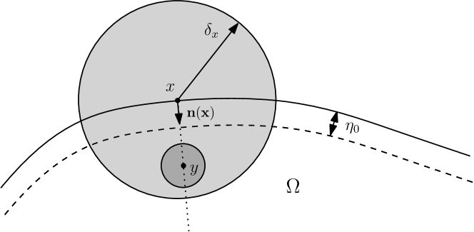
Fig. 3: Cover of $\partial\Omega$.

Under the assumption that the boundary $\partial\Omega$ is $C^{2}$ smooth, as shown in Fig. 3, for any point $\bm{x}\in\partial\Omega$, there exists $\delta_{\bm{x}}>0$ such that

$$U_{\bm{x}}=\{\mathbf{z}\in\Omega:|\mathbf{z}-\bm{x}|<\delta_{\bm{x}}\}$$

is star-shaped with respect to open ball $B(\bm{y},\delta_{\bm{x}}/4)$ with $\bm{y}=\bm{x}-\frac{2}{3}\delta_{\bm{x}}\mathbf{n}(\bm{x})$, $\mathbf{n}(\bm{x})$ is the outer normal of $\partial\Omega$ at $\bm{x}$.

$\displaystyle\bigcup_{\bm{x}\in\partial\Omega}U_{\bm{x}}$ is an open cover of $\partial\Omega$. Since $\partial\Omega$ is compact, there exist $\bm{x}_{k}\in\partial\Omega,\;k=1,\cdots,N$ such that

$$\partial\Omega\subset\bigcup_{k=1}^{N}U_{\bm{x}_{k}}.$$

Compactness of $\partial\Omega$ also implies that there exists $\displaystyle\eta_{0}\in\left(0,\frac{1}{2}\min_{1\leq k\leq N}\delta_{\bm{x}_{k}}\right)$ such that

$$\mathcal{V}_{\eta_{0}}\subset\bigcup_{k=1}^{N}U_{\bm{x}_{k}}.$$

Recall that $\mathcal{V}_{\eta_{0}}=\{\bm{x}\in\Omega:\mbox{dist}(\bm{x},\partial\Omega)\leq\eta_{0}\}$.

For any $0\leq\eta\leq\eta_{0}/2$,

$$U_{\bm{x}_{k}}^{\eta}=\{\mathbf{z}\in\Omega_{\eta}:|\mathbf{z}-\bm{x}_{k}|<\delta_{\bm{x}_{k}}\},\quad k=1,\cdots,N$$

are also star-shaped with respect to $B(\bm{y}_{k},\delta_{\bm{x}_{k}}/4)$ with $\bm{y}_{k}=\bm{x}_{k}-\frac{2}{3}\delta_{\bm{x}_{k}}\mathbf{n}(\bm{x}_{k})$, $\mathbf{n}(\bm{x}_{k})$ is the outer normal of $\partial\Omega$ at $\bm{x}_{k}$.

On the other hand, compactness of $\bar{\Omega}_{\eta_{0}}$ gives $\mathbf{z}_{1},\cdots,\mathbf{z}_{M}\in\bar{\Omega}_{\eta_{0}}$ such that

$$\bar{\Omega}_{\eta_{0}}\subset\bigcup_{k=1}^{M}B(\mathbf{z}_{k},\eta_{0}/2).$$

For any $0\leq\eta\leq\eta_{0}/2$,

$$\Omega_{\eta}=\left(\bigcup_{k=1}^{N}U_{\bm{x}_{k}}^{\eta}\right)\bigcup\left(\bigcup_{k=1}^{M}B(\mathbf{z}_{k},\eta_{0}/2)\right)$$

$U_{\bm{x}_{k}}^{\eta}$ is star-shaped with respect to $B(\bm{y}_{k},\eta_{0}/2)$ and $B(\mathbf{z}_{k},\eta_{0}/2)$ is star-shaped with respect to itself. It is easy to check based on above decomposition, Theorem 10 implies (3.11) and (4.16).

References

- [1] J. Beale and A. Majda. High order accurate vortex methods with explicit velocity kernels. Journal of Computational Physics, 58:188–208, 1985.
- [2] M. Belkin and P. Niyogi. Laplacian eigenmaps for dimensionality reduction and data representation. Neural Computation, 15(6):1373–1396, 2003.
- [3] A. Chertock. A practical guide to deterministic particle methods. handbook of nu- merical analysis. Handbook of Numerical Analysis, 18:177–202, 2017.
- [4] P. T. Choi, K. C. Lam, and L. M. Lui. Flash: Fast landmark aligned spherical harmonic parameterization for genus-0 closed brain surfaces. SIAM Journal on Imaging Sciences, 8:67–94, 2015.
- [5] A. Cohen and B. Perthame. Optimal approximations of transport equations by particle and pseudoparticle methods. SIAM J. Math. Anal., 32:616–636, 2000.
- [6] R. R. Coifman, S. Lafon, A. B. Lee, M. Maggioni, F. Warner, and S. Zucker. Geometric diffusions as a tool for harmonic analysis and structure definition of data: Diffusion maps. In Proceedings of the National Academy of Sciences, pages 7426–7431, 2005.
- [7] G. Cottet and P. Koumoutsakos. Vortex Methods Theory and Practice. Cambridge Univ. Press, 2000.
- [8] T. K. Dey, J. Sun, and Y. Wang. Approximating cycles in a shortest basis of the first homology group from point data. Inverse Problems, 27(12):124004, 2011.
- [9] Q. Du. Nonlocal Modeling, Analysis, and Computation. SIAM, 2019.
- [10] Q. Du, M. Gunzburger, R. B. Lehoucq, and K. Zhou. Analysis and approximation of nonlocal diffusion problems with volume constraints. SIAM Review, 54:667–696, 2012.
- [11] Q. Du, L. Ju, L. Tian, and K. Zhou. A posteriori error analysis of finite element method for linear nonlocal diffusion and peridynamic models. Math. Comp., 82:1889–1922, 2013.
- [12] Q. Du, T. Li, and X. Zhao. A convergent adaptive finite element algorithm for nonlocal diffusion and peridynamic models. SIAM J. Numer. Anal., 51:1211–1234, 2013.
- [13] Q. Du and X. Tian. Mathematics of smoothed particle hydrodynamics: A study via nonlocal Stokes equations. Foundations of Computational Mathematics, 20(4):801–826, 2020.
- [14] Q. Du, X. Tian, C. Wright, and Y. Yu. Nonlocal trace spaces and extension results for nonlocal calculus. arXiv preprint arXiv:2107.00177, 2021.
- [15] J. Eldredge, A. Leonard, and T. Colonius. A general deterministic treatment of deriva- tives in particle methods. J. Comput. Phys., 180:686–709, 2002.
- [16] L. C. Evans. Partial Differential Equations. American Mathematical Society, 1997.
- [17] G. Galdi. An Introduction to the Mathematical Theory of the Navier-Stokes Equations: Steady-State Problem. Springer, 2011.
- [18] R. A. Gingold and J. J. Monaghan. Smoothed particle hydrodynamics: theory and appli- cation to non-spherical stars. Monthly Notices Royal Astronomical Society, 181:375–389, 1977.
- [19] X. Gu, Y. Wang, T. F. Chan, P. M. Thompson, and S.-T. Yau. Genus zero surface conformal mapping and its application to brain surface mapping. IEEE TMI, 23:949–958, 2004.
- [20] C.-Y. Kao, R. Lai, and B. Osting. Maximization of laplace-beltrami eigenvalues on closed riemannian surfaces. ESAIM: Control, Optimisation and Calculus of Variations, 23:685–720, 2017.
- [21] P. Koumoutsakos. Multiscale flow simulations using particles. Annu. Rev. Fluid Mech., 37:457–487, 2005.
- [22] R. Lai, Z. Wen, W. Yin, X. Gu, and L. Lui. Folding-free global conformal mapping for genus-0 surfaces by harmonic energy minimization. Journal of Scientific Computing, 58:705–725, 2014.
- [23] R. Lai and H. Zhao. Multi-scale non-rigid point cloud registration using robust sliced-wasserstein distance via laplace-beltrami eigenmap. SIAM Journal on Imaging Sciences, 10:449–483, 2017.
- [24] H. Lee and Q. Du. Nonlocal gradient operators with a nonspherical interaction neighborhood and their applications. ESAIM: Mathematical Modelling and Numerical Analysis, 54(1):105–128, 2020.
- [25] Z. Li, Z. Shi, and J. Sun. Point integral method for solving poisson-type equations on manifolds from point clouds with convergence guarantees. Communications in Computational Physics, 22(1):228–258, 2017.
- [26] Z. Li, Z. Shi, and J. Sun. Point integral method for elliptic equations with variable coefficients on point cloud. Communications in Computational Physics, 26(2):506–530, 2019.
- [27] M. Liu and G. Liu. Smoothed particle hydrodynamics (sph): an overview and recent developments. Arch Comput Methods Eng., 17:25–76, 2010.
- [28] L. Lucy. A numerical approach to the testing of the fission hypothesis. Astron J., 82:1013–1024, 1977.
- [29] T. W. Meng, P. T. Choi, and L. M. Lui. Tempo: Feature-endowed teichmuller extremal mappings of point clouds. SIAM Journal on Imaging Sciences, 9:1582–1618, 2016.
- [30] T. Mengesha and Q. Du. Nonlocal constrained value problems for a linear peridynamic Navier equation. Journal of Elasticity, 116(1):27–51, 2014.
- [31] T. Mengesha and Q. Du. Characterization of function spaces of vector fields and an application in nonlinear peridynamics. Nonlinear Analysis, 140:82–111, 2016.
- [32] J. Monaghan. Smoothed particle hydrodynamics. Rep. Prog. Phys., 68:1703–1759, 2005.
- [33] S. Osher, Z. Shi, and W. Zhu. Low dimensional manifold model for image processing. SIAM Journal on Imaging Sciences, 10:1669–1690, 2017.
- [34] G. Peyré. Manifold models for signals and images. Computer Vision and Image Understanding, 113:248–260, 2009.
- [35] M. Reuter, F. E. Wolter, and N. Peinecke. Laplace-beltrami spectra as ’shape-dna’ of surfaces and solids. Computer Aided Design, 38:342–366, 2006.
- [36] Z. Shi. Enforce the dirichlet boundary condition by volume constraint in point integral method. Commun. Math. Sci., 15(6):1743–1769, 2017.
- [37] Z. Shi and J. Sun. Convergence of the point integral method for poisson equation on point cloud. Research in the Mathematical Sciences, 4, 2017.
- [38] S. Silling. Reformulation of elasticity theory for discontinuities and long-range forces. J. Mech. Phys. Solids, 48:175–209, 2000.
- [39] X. Tian and Q. Du. Asymptotically compatible schemes and applications to robust discretization of nonlocal models. SIAM J. Numerical Analysis, 52:1641–1665, 2014.
- [40] A. Tornberg and B. Engquist. Numerical approximations of singular source terms in differential equations. Journal of Computational Physics, 200:462–488, 2004.
- [41] T. W. Wong, L. M. Lui, X. Gu, P. Thompson, T. Chan, and S.-T. Yau. Instrinic feature extraction and hippocampal surface registration using harmonic eigenmap. Technical Report, UCLA CAM Report 11-65, 2011.
- [42] Y. Zhang, Z. Shi, and Q. Du. Nonlocal Stokes equation with relaxation on the divergence free equation. Preprint, 2021.
- [43] K. Zhou and Q. Du. Mathematical and numerical analysis of linear peridynamic models with nonlocal boundary conditions. SIAM J. Numer. Anal., 48:1759–1780, 2010.