Holographic QCD₃ and Chern-Simons theory from anisotropic supergravity

Abstract

Based on the gauge-gravity duality, we study the three-dimensional QCD (QCD₃) and Chern-Simons theory by constructing the anisotropic black D3-brane solution in IIB supergravity. The deformed bulk geometry is obtained by performing a double Wick rotation and dimension reduction which becomes an anisotropic bubble configuration exhibiting confinement in the dual theory. And its anisotropy also reduces to a Chern-Simons term due to the presence of the dissolved D7-branes or the axion field in bulk. Using the bubble geometry, we investigate the the ground-state energy density, quark potential, entanglement entropy and the baryon vertex according to the standard methods in the AdS/CFT dictionary. Our calculation shows that the ground-state energy illustrates degenerate to the Chern-Simons coupling coefficient which is in agreement with the properties of the gauge Chern-Simons theory. The behavior of the quark tension, entanglement entropy and the embedding of the baryon vertex further implies strong anisotropy may destroy the confinement. Afterwards, we additionally introduce various D7-branes as flavor and Chern-Simons branes to include the fundamental matter and effective Chern-Simons level in the dual theory. By counting their orientation, we finally obtain the associated topological phase in the dual theory and the critical mass for the phase transition. Interestingly the formula of the critical mass reveals the flavor symmetry, which may relate to the chiral symmetry, would be restored if the anisotropy increases greatly. As all of the analysis is consistent with characteristics of quark-gluon plasma, we therefore believe our framework provides a remarkable way to understand the features of Chern-Simons theory, the strong coupled nuclear matter and its deconfinement condition with anisotropy.

Si-wen Li, Sen-kai Luo, Ya-qian Hu,

1 Introduction

While quantum chromodynamics (QCD) is the underlying theory to describe the strong interaction, it is usually very difficult to solve at low energy due to its asymptotic freedom, especially in the dense matter with finite temperature. Therefore it provides motivation to study the dynamics of strongly coupled non-Abelian gauge field theory via the gauge-gravity duality as an alternative option [1, 2]. On the other hand, the heavy-ion collision (HIC) experiments show that quark-gluon plasma (QGP) created in the collision is strongly coupled [3, 4] and anisotropic [5, 6, 7, 8], hence constructing the type IIB supergravity in order to investigate the anisotropic and strongly coupled QGP or Yang-Mills theory through gauge-gravity duality is naturally significant [9, 10, 11] since, as it has been well-known, the most famous example in the gauge-gravity duality is the corresponding between four-dimensional $\mathcal{N}=4$ $SU\left(N_{c}\right)$ super Yang-Mills theory on $N_{c}$ D3-branes and type IIB super string theory on $\mathrm{AdS_{5}}\times S^{5}$.

A remarkable work in the top-down holographic approach to study the anisotropy in gauge theory is [12] in which the black D3-brane solution in type IIB supergravity is anisotropic due to the presence of the axion field or dissolved D7-branes in the bulk. Following the AdS/CFT dictionary, the thermodynamics and transport properties in an anisotropic plasma are explored holographically by the gravity solution in [12] which attracts many interests [13, 14]. In particular, another concern in [12] is that the presented axion field leads to a theta term $\theta\int F\wedge F$ in the dual theory and the $\theta$ parameter is spatially dependent. Since $\theta$-dependence involves the topological property in gauge theory, it also gets many attentions in theoretical and phenomenological researches [15]. Although the experimental value of the $\theta$ parameter is very small, it may influence many observable effects in gauge theories e.g. the deconfinement phase transition [16, 17], the glueball spectrum [18], the CP violation in hot QCD [19, 20], the chiral magnet effect [21, 22], the large N limit [23] and its holographic correspondence [24, 25, 26, 27]. Accordingly, the holographic duality proposed in [12] becomes a topical issue at one stage.

Keeping these in hand, in this work, we would like to study the holographic duality between the three-dimensional QCD (QCD₃) and Chern-Simons theory based on [12]. As the $\theta$ parameter in the framework of [12] linearly depends on one of the three spatial coordinates, integrating by parts, one can get a three-dimensional Chern-Simons term as $\theta\int F\wedge F\sim\int dz\wedge\mathrm{Tr}\left(A\wedge F+\frac{2}{3}A^{3}\right)$ which accordingly is the part of the motivation for this work. Furthermore, QCD₃ or the Chern-Simons theory involving fundamental matters with $N_{f}$ flavors and their large N ’t Hooft limit are also interesting topics especially in three-dimensional case [28, 29, 30, 31, 32, 33, 34], thus including flavors would also be our concern in this project. And the presented anisotropy might be more closed to the realistic physical situation in some materials.

However one of the key points here is to find a scheme to combine the gravity system in [12] with the three-dimensional theory in holography. Fortunately the answer could be found in the famous [35, 36] which provides the compactification in the D3-branes system in order to obtain a three-dimensional non-supersymmetric and non-conformal gauge theory, as it is successfully performed in the D4/D8 approach [37]. So by imposing the compactification method in [35, 36] to the supergravity system in [12], in this work we first obtain the bubble configuration of the bulk geometry which could be remarkably analytical if we take the compactification limit (i.e. the size of the compactification direction vanishes). Since the bubble configuration does not have a horizon, the dual theory is at zero temperature limit. And we examine the dual theory by introducing a probe D3-brane at the holographic boundary which exactly exhibits a Yang-Mills plus Chern-Simons theory as it is expected. A notable feature in our holographic setup is that the Chern-Simons level is naturally identified to the number of the D7-branes dissolved in the bulk which is automatically quantized. And we believe this provides a holographic proof to the quantization of the Chern-Simons level.

Afterwards, some of the observables are investigated by using the standard method according to the AdS/CFT dictionary in the bubble configuration of the bulk, specifically they are the ground-state energy density, quark potential, entanglement entropy and the baryon vertex. To simplify the calculation, we consider that the size of the compacted direction trends to be vanished in the bulk geometry throughout this work, so that the dual theory would become exactly three-dimensional. Then our results show that the ground-state energy is degenerate to the Chern-Simons coupling coefficient which is in agreement with the properties of the gauge transformation in the gauge Chern-Simons theory [38]. Besides, the behaviors of the quark potential and entanglement entropy depending on the position of the fundamental string or “slab” resultantly reveal that the confinement may be destroyed in hadron if the anisotropy becomes strong enough, because the entanglement entropy may also be a characteristic tool to detect the confinement [39, 40, 41, 42]. Moreover, we introduce a wrapped D5-brane on $S^{5}$ as the baryon vertex [43] in this geometry and study its embedding configuration as [44]. The numerical calculation confirms the wrapped configuration of the baryon vertex in this system and the D-brane force illustrates the bottom of the bulk is the stable position of a baryon vertex as it is expected to minimize its energy. Interestingly, the numerical calculation also displays the wrapped baryon vertex trends to become unwrapped by the increasing of the anisotropy which means the baryon vertex may not stably exist if the anisotropy becomes very large. And it is seemingly consistent with the analysis of the quark potential and entanglement entropy with respect to the confinement in this system i.e. strong anisotropy may destroy the confinement.

Last but not least, to explore the Chern-Simons topological feature involving the flavors in the dual theory, following [45, 46, 47], various D7-branes as flavor and Chern-Simons branes are introduced into the bulk bubble configuration as probes. In a transverse plane, the vacuum configuration of the D7-branes, which means the embedding function minimizes the energy of the D7-branes, is numerically evaluated and the calculation shows the vacuum structure is shifted by the presence of the axion field in the bulk. To further consider the spontaneous breaking of the flavor symmetry $U\left(N_{f}\right)$, we separate coincident $p$ of $N_{f}$ flavor branes living into the upper part of the transverse plane and the other coincident $N_{f}-p$ flavor branes living into the lower part of the plane while they extend to a same position at the holographic boundary. Therefore the interpretation of such configuration could be that the flavor symmetry $U\left(N_{f}\right)$ spontaneously breaks down into $U\left(p\right)\times U\left(N_{f}-p\right)$ at low energy in dual theory. Taking into account the contribution of the orientation of the flavor and Chern-Simons branes, we can get an effective flavor-dependent Chern-Simons level. Then evaluating the total energy including both flavor and Chern-Simons branes by counting the orientation in the effective Chern-Simons level, the associated topological phases in the dual theory can be obtained. A noteworthy conclusion here is that the total energy including flavor and Chern-Simons branes illustrates the topological phase transition may occur at a critical flavor mass $m^{*}$ which decreases due to the presence of the anisotropy or the axion field in the bulk geometry. By analyzing the phase diagram, it seemingly means the broken flavor symmetry $U\left(p\right)\times U\left(N_{f}-p\right)$, which may relates to the chiral symmetry, would become restored to $U\left(N_{f}\right)$ if the anisotropy becomes sufficiently strong. And this behavior is also predicted by the numerical evaluation of the embedding of the flavor branes since the two branches of the flavor branes trend to become coincident when the anisotropy becomes large. Altogether, this framework may provide a holographic way to study the behavior of metastable vacua in large N QCD₃ with a Chern-Simons term [48] and its deconfined condition with anisotropy, although the anisotropy is expected to be small for the numerical calculations in this project.

The outline of this manuscript is as follows. In Section 2, we briefly review the anisotropic black brane solution in the type IIB supergravity, then give our holographic setup to this work. In Section 3, we calculate several observables with respect to the constructed bulk geometry. In Section 4, we discuss the embedding of the flavor and Chern-Simons branes. In Section 5, we analyze the corresponding topological phase and its associated phase transition in holography. Summary and discussion are given in the final section. In addition, we list the relevant parts of the functions presented in the bulk geometry in the appendix which would be very useful to this work.

2 Holographic setup

2.1 Review of the anisotropic solution in type IIB supergravity

In this subsection, we review and collect the relevant content of the anisotropic solution in ten-dimensional type IIB supergravity in [12]. The remarkable anisotropic solution describes the bulk dynamics of $N_{c}$ D3-branes with $N_{\mathrm{D7}}$ D7-branes dissolved in the spacetime in the large $N_{c}$ limit and the D-brane configuration is given in Table 1.

Black brane background	$t$	$x$	$y$	$z$	$u$	$\Omega_{5}$
$N_{c}$ D3-branes	-	-	-	-
$N_{\mathrm{D7}}$ D7-branes	-	-	-			-

Table 1: The configuration of the D-branes in the black brane background. “-” represents the D-brane extends along the direction.

As our concern would be the holographic duality, let us start with the type IIB supergravity action in string frame,

$$S_{\mathrm{IIB}}=\frac{1}{2\kappa_{10}^{2}}\int d^{10}x\sqrt{-g}\left[e^{-2\phi}\left(\mathcal{R}+4\partial_{M}\phi\partial^{M}\phi\right)-\frac{1}{2}F_{1}^{2}-\frac{1}{4\cdot 5!}F_{5}^{2}\right],$$ (2.1)

where the index $M$ runs over 0 to 9, $\kappa_{10}$ is the ten-dimensional gravitational coupling constant $2\kappa_{10}^{2}=\left(2\pi\right)^{7}l_{s}^{8}$. To obtain an anisotropic solution, the associated equation of motion to (2.1) can be solved by the following anisotropic ansatz in string frame,

$$ds^{2} =\frac{L^{2}}{u^{2}}\left(-\mathcal{F}\mathcal{B}dt^{2}+dx^{2}+dy^{2}+\mathcal{H}dz^{2}+\frac{du^{2}}{\mathcal{F}}\right)+L^{2}\mathcal{Z}d\Omega_{5}^{2},$$

$$F_{1} =d\chi,\ \chi=az,\ F_{5}=dC_{4}=\frac{4}{L}\left(\Omega_{S^{5}}+\star\Omega_{S^{5}}\right),$$

$$\mathcal{H} =e^{-\phi},\ \mathcal{Z}=e^{\frac{1}{2}\phi},$$ (2.2)

where $\chi,\phi,\Omega_{S^{5}}$ refers to the axion, dilaton and the unit volume form of a five-sphere $S^{5}$. The parameters in the solution are given as follows,

$$L^{4}=4\pi g_{s}N_{c}l_{s}^{4}=\lambda l_{s}^{4},a=\frac{\lambda n_{\mathrm{D7}}}{4\pi N_{c}},$$ (2.3)

where $L,g_{s},\lambda$ represents the radius of the bulk, the string coupling and the ’t Hooft coupling constant respectively. The solution (2.2) describes the black branes with a horizon at $u=u_{H}$ and the anisotropy in $z$ direction. There would not be new field in the boundary which is located at $u=0$ because the $N_{\mathrm{D7}}$ D7-branes do not extend along the holographic direction $u$. Since the dynamic of the axion $\chi$, which magnetically couples to $N_{\mathrm{D7}}$ D7-branes, is taken into account, it is clear that the supergravity solution (2.2) includes the backreaction of $N_{\mathrm{D7}}$ D7-branes to the D3-brane bulk geometry. We note that the $N_{\mathrm{D7}}$ D7-branes are distributed along $z$ direction with the constant distribution density $n_{\mathrm{D7}}=dN_{\mathrm{D7}}/dz$ according to the solution for $\chi$. So once the backreaction of $N_{\mathrm{D7}}$ D7-branes to the background geometry is included, it implies that $N_{\mathrm{D7}}/N_{c}$ is fixed in the large $N_{c}$ limit.

The regular functions $\mathcal{F},\mathcal{B},\phi$ in (2.2) depend on the holographic coordinate $u$ which must be determined by their equations of motion. However they are non-analytical in general. In order to avoid the conical singularities in the bulk, the Euclidean version of the bulk metric near the horizon,

$$ds_{E}^{2}\simeq\frac{1}{u_{H}^{2}}\left[\mathcal{F}_{1}\left(u_{H}\right)\mathcal{B}\left(u_{H}\right)\left(u-u_{H}\right)\left(dt_{E}\right)^{2}+\frac{du^{2}}{\mathcal{F}_{1}\left(u-u_{H}\right)}\right],\ \mathcal{F}_{1}=-\frac{d\mathcal{F}}{du},$$ (2.4)

must impose the period $\delta t_{E}$ to be $2\pi$. Hence it reduces to the formula of the Hawking temperature $T$ as,

$$\delta t_{E}=\frac{4\pi}{\mathcal{F}_{1}\left(u_{H}\right)\sqrt{\mathcal{B}_{H}}}=\frac{1}{T}.$$ (2.5)

Suppose the temperature is sufficiently large $T\rightarrow\infty$ (or equivalently $\delta t_{E}\rightarrow 0$), the functions $\mathcal{F},\mathcal{B},\phi$ can be analytically written as the series of $a$ which are given in the Appendix. We note this high-temperature analysis would be remarkably useful in the following sections of this work.

2.2 Construction for the 2+1 dimensional theory

As it is known that the type IIB supergravity theory holographically corresponds to the $\mathcal{N}=4$ super Yang-Mills theory on D3-brane, it would be very straightforward to construct the D3-brane configuration or the $\mathcal{N}=4$ super Yang-Mills theory in order to obtain a non-supersymmetric and non-conformal dual theory by following the steps in the well-known [35, 36]. Specifically the first step is to take the spatial dimensions $y$ of the D3-brane to be compactified on a circle $S^{1}$ with a period $\delta y$. Therefore the dual theory is effectively three-dimensional below the Kaluza-Klein energy scale defined as $M_{KK}=2\pi/\delta y$. The second step is going to get rid of all massless fields other than the gauge fields, which is to impose respectively the periodic and anti-periodic boundary condition on bosonic and fermionic fields along $S^{1}$. Afterwards the supersymmetric fermions and scalars acquire mass of order $M_{KK}$ thus they are decoupled in the low-energy dynamics. So the dual theory below $M_{KK}$ becomes three-dimensional pure gauge theory. By keeping these in mind, the next step is to identify the bulk geometry that corresponds to this gauge theory. The answer can be found by interchanging the roles of $t$ and $y$ i.e. performing a double Wick rotation $t\rightarrow-iy,y\rightarrow-it$ to the metric presented in (2.2), which is

$$ds^{2}=\frac{L^{2}}{u^{2}}\left(-dt^{2}+dx^{2}+\mathcal{H}dy^{2}+\mathcal{F}\mathcal{B}dz^{2}+\frac{du^{2}}{\mathcal{F}}\right)+L^{2}\mathcal{Z}d\Omega_{5}^{2},$$ (2.6)

where we have renamed $y,z$ after the double Wick rotation. We note that in this notation the axion field becomes,

$$\chi=ay,$$ (2.7)

while $\phi,F_{5}$ remains and now $z$ is periodic as,

$$\delta z=\frac{4\pi}{\mathcal{F}_{1}\left(u_{KK}\right)\sqrt{\mathcal{B}\left(u_{KK}\right)}}=\frac{2\pi}{M_{KK}}.$$ (2.8)

Using the formulas given in the appendix, we can obtain

$$M_{KK}=\frac{2}{u_{KK}}+\frac{u_{KK}}{24}\left(5\log 2-2\right)a^{2}+\mathcal{O}\left(a^{4}\right).$$ (2.9)

The solution (2.6) represents a bubble geometry of the bulk which is anisotropic on $\left\{x,y\right\}$ plane and defined only for $0\leq u\leq u_{KK}$. The D-brane configuration for the bubble solution (2.6) is given in Table 2.

Bubble background	$t$	$x$	$y$	$\left(z\right)$	$u$	$\Omega_{5}$
$N_{c}$ D3-branes	-	-	-	-
$N_{\mathrm{D7}}$ D7-branes	-	-		-		-

Table 2: The configuration of the D-branes in the bubble solution (2.6).

Here we have renamed $u_{H}$ as $u_{KK}$ since there is not a horizon in the bulk as it is illustrated in Figure 1.

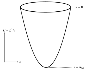
Figure 1: The bubble geometry of the $N_{c}$ D3-brane. The bulk ends at $u=u_{KK}$ and the holographic boundary is located at $u=0$. We note that the standard holographic radius coordinate is in fact defined as $U=L^{2}/u$, so the bubble configuration is exactly illustrated in the $\left\{U,z\right\}$ plane.

Since the wrap factor $L^{2}/u^{2}$ never goes to zero, the dual theory would exhibit confinement according to the behavior of the Wilson loop in this bulk geometry. Besides, we can notice that the gauge theory on D3-brane becomes purely three-dimensional theory if the compactified direction $z$ shrinks to zero i.e. $\delta z\rightarrow 0$ or $M_{KK}\rightarrow\infty$. And this limit exactly corresponds to the high temperature limit in the black brane solution (2.2) so that in the limit of $\delta z\rightarrow 0$, the functions $\mathcal{F},\mathcal{B},\phi$ in (2.6) are also analytical as they are given in the appendix. Accordingly we are going to consider the case in the limit $\delta z\rightarrow 0$ throughout this work since our concern is the three-dimensional dual theory exactly.

2.3 The dual theory

The dual theory with respect to the bulk solution (2.6) is defined at the zero temperature limit $T\rightarrow 0$ since there is not a horizon i.e. $\delta t\rightarrow\infty$. To examine the dual theory, let us introduce a single probe D3-brane located at the boundary $u\rightarrow 0$. As we have discussed, in the bubble geometry (2.6), the low-energy modes in the dual field theory contain the gauge field only, so the effective action for such a probe D3-brane is given as,

$$S_{\mathrm{D3}}=-T_{3}\mathrm{Tr}\int d^{3}xdze^{-\phi}\sqrt{-\det\left(g_{ab}+\mathcal{F}_{ab}\right)}+\frac{1}{2}T_{3}\mathrm{Tr}\int\chi\mathcal{F}\wedge\mathcal{F},$$ (2.10)

where the tension of the D3-brane is given as $T_{3}=\left(2\pi\right)^{-3}l_{s}^{-4}g_{s}^{-1}$. And $g_{ab},\mathcal{F}_{ab}=2\pi\alpha^{\prime}F_{ab}$ is the induced metric and the gauge field strength on the worldvolume of the D3-brane. Assuming $\mathcal{F}_{ab}$ does not have components along $z$ and does not depend on $z$, then the quadratic expansion of the action (2.10) is

$$S_{\mathrm{D3}} =-\frac{1}{4}T_{3}\left(2\pi\alpha^{\prime}\right)^{2}\mathrm{Tr}\int_{\mathrm{D3}}d^{3}xdz\sqrt{-g}e^{-\phi}g^{ac}g^{bd}F_{ab}F_{cd}-\mu_{3}\left(2\pi\alpha^{\prime}\right)^{2}\mathrm{Tr}\int_{\mathrm{D3}}d\chi\wedge\omega_{3}$$

$$=-\frac{N_{c}}{4\lambda_{3}}\mathrm{Tr}\int_{\mathbb{R}^{2+1}}d^{3}xF_{ab}^{2}-\frac{N_{\mathrm{D7}}}{4\pi}\mathrm{Tr}\int_{\mathbb{R}^{2+1}}\omega_{3},$$ (2.11)

where $\lambda_{3}=\lambda M_{KK}/\left(2\pi\right)$ is the three-dimensional ’t Hooft coupling constant and

$$\omega_{3}=A\wedge dA+\frac{2}{3}A\wedge A\wedge A,$$ (2.12)

is the Chern-Simons three-form. We use $A$ to denote the gauge potential and have imposed the boundary value $\phi_{\mathrm{bdry}}=0,\mathcal{F}_{\mathrm{bdry}}=\mathcal{B}_{\mathrm{bdry}}=1$ to (2.11). Clearly the dual theory on the D3-brane is effectively three-dimensional Yang-Mills plus Chern-Simons theory below the energy scale $M_{KK}$. Notice that the dual theory is expected to be purely three-dimensional theory if we take the limit $\delta z\rightarrow 0$ or equivalently $M_{KK}\rightarrow\infty$.

It is remarkable to notice that in this holographic setup, the level number of the Chern-Simons term $N_{\mathrm{D7}}$ is integer automatically since the level number is exactly the number of D7-branes in the gravity side. This leads to a proof of the quantization of the Chern-Simons level via holography. On the other hand, when the backreaction of the $N_{\mathrm{D7}}$ D7-branes is included in the bulk, the dual theory is equivalently a topological massive theory. This can be confirmed once we derive the formula of the propagator with respect to action (2.11) which is [38],

$$\Delta_{ab}=\frac{p^{2}\eta_{ab}-p_{a}p_{b}+i\kappa g_{YM}^{2}\epsilon_{abc}p^{c}}{p^{2}\left(p^{2}-\kappa^{2}g_{YM}^{2}\right)}+\mathrm{gauge\ fixing\ terms},$$ (2.13)

where $\kappa=N_{\mathrm{D7}}/\left(4\pi\right)$ and we use $p$ to denote the momentum in 2+1 dimensional spacetime. Therefore, the propagator defines the topological mass of the gauge field via the pole $p^{2}=\kappa^{2}g_{YM}^{2}$ which is determined by the numbers of D7-branes. Thus the presented D7-branes involve the topological properties of the dual theory and, we will see, they contribute to the various vacuum configurations in the dual theory.

3 Observables

In this section, we will extract relevant information on the physics of the Yang-Mills theory with a Chern-Simons term dual to the anisotropic background given in (2.6). Using the standard holographic methods, we will focus on the ground-state energy, quark potential, entanglement entropy and baryon vertex in this system.

3.1 The ground-state energy

In the holographic dictionary, one of the basic entries is the relation between the renormalized on-shell supergravity action and partition function of the dual field theory [1, 2, 35, 36]. Therefore the ground-state energy density $f$ of the dual field theory can be obtained through the relation

$$Z=e^{-V_{3}f}=e^{-S_{E,\mathrm{on-shell}}^{ren}},$$ (3.1)

where $V_{3}$ refers to the infinite three-dimensional Euclidean spacetime volume. $S_{E,\mathrm{on-shell}}^{ren}$ is the renormalized on-shell action for type IIB supergravity, which is given by

$$S_{E,\mathrm{on-shell}}^{ren}=S_{\mathrm{IIB}}^{E}+S_{\mathrm{GH}}+S_{\mathrm{CT}},$$ (3.2)

where $S_{\mathrm{GH}},S_{\mathrm{CT}}$ refers to the Gibbons-Hawking term and holographic counterterm for the type IIB supergravity. $S_{\mathrm{IIB}}^{E}$ refers to the Euclidean version of (2.1) which in Einstein frame is given as,

$$S_{\mathrm{IIB}}^{E}=-\frac{1}{2\kappa^{2}}\int_{\mathcal{M}}d^{10}x\sqrt{g}\left[\mathcal{R}-\frac{1}{2}\partial_{M}\phi\partial^{M}\phi-\frac{1}{2}e^{2\phi}F_{1}^{2}-\frac{1}{4\cdot 5!}F_{5}^{2}\right].$$ (3.3)

Since only $F_{5}$ has components on $\Omega_{5}$, the onshell action $S_{\mathrm{IIB}}^{E}$ can be integrated out over $\Omega_{5}$ to become an effective five-dimensional action as,

$$S_{\mathrm{IIB}}^{E}=\frac{1}{2\kappa_{5}^{2}}\int_{\mathcal{M}}d^{5}x\sqrt{g}\left(\mathcal{R}^{\left(5\right)}-2\Lambda-\frac{1}{2}\partial_{M}\phi\partial^{M}\phi-\frac{1}{2}e^{2\phi}\partial_{M}\chi\partial^{M}\chi\right),$$ (3.4)

where $M$ runs over 0 to 4. The cosmological constant is $\Lambda=-6/L^{2}$, $\mathcal{R}^{\left(5\right)}$ is the five-dimensional scalar curvature and $\kappa_{5}$ is the five-dimensional gravitational coupling constant. The action (3.4) is nothing but the five-dimensional axion-dilaton-gravity action. Hence the holographic counterterm can be chosen as [12],

$$S_{\mathrm{CT}}=-\frac{1}{\kappa_{5}^{2}}\int_{\partial\mathcal{M}}d^{4}x\sqrt{h}\left(3-\frac{1}{8}e^{2\phi}h^{\mu\nu}\partial_{\mu}\chi\partial_{\nu}\chi\right)+\log v\int_{\partial\mathcal{M}}d^{4}x\sqrt{h}\mathcal{A}-\frac{1}{4}\left(c_{\mathrm{sch}}-1\right)\int_{\partial\mathcal{M}}d^{4}x\mathcal{A},$$ (3.5)

where $h_{\mu\nu}$ refers to the boundary metric and $\mathcal{A}\left(h_{\mu\nu},\phi,\chi\right)$ refers to the conformal anomaly in the axion-dilaton-gravity system . In this sense, the metric near the boundary is required to take the form as,

$$ds^{2}=\frac{dv^{2}}{v^{2}}+h_{\mu\nu}dx^{\mu}dx^{\nu}.$$ (3.6)

in which the coordinate $v$ is the standard Fefferman-Graham (FG) coordinate. The relation between the coordinate $u$ presented in (2.6) and the FG coordinate is collected as,

$$u=v+\frac{a^{2}}{12}v^{3}+\mathcal{O}\left(v^{5}\right),v=u-\frac{a^{2}}{12}u^{3}+\mathcal{O}\left(u^{5}\right).$$ (3.7)

We also note that the standard Gibbons-Hawking term is given by the trace of the extrinsic curvature $K$ of the boundary as

$$S_{\mathrm{GH}}=\frac{1}{\kappa_{5}^{2}}\int_{\partial\mathcal{M}}\sqrt{h}K.$$ (3.8)

Plugging (3.4) (3.5) (3.8) into (3.2) and using the relation (3.1), the resultant free energy density of the dual theory is computed up to $\mathcal{O}\left(a^{2}\right)$ as,

$$f=-\frac{M_{KK}^{3}N_{c}^{2}}{64\pi}+\frac{a^{2}M_{KK}N_{c}^{2}}{64\pi}+\mathcal{O}\left(a^{4}\right).$$ (3.9)

The free energy density depending on $a$ implies the ground-state is degenerate to the Chern-Simons coupling coefficient $\kappa=N_{\mathrm{D7}}/\left(4\pi\right)$. Since $a\sim dN_{\mathrm{D7}}/dy$ is the distribution density of the $N_{\mathrm{D7}}$ D7-branes, the value of $a$ could be same for different $\kappa$. Therefore the (3.9) describes the vacuum energy in various branches characterized by its level number $4\pi\kappa$. To any given interval, we fix the length $1/\left(4\pi\right)$ of $a$ for possible values of $\kappa$, then the ground-state free energy (3.9), which implies the vacuum with distinct $\kappa$, is shown in Figure 2.

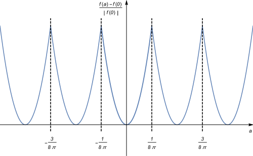
Figure 2: The vacuum energy for distinct $\kappa$. For example for $\kappa=0$, we have $a\in\left[-\frac{1}{8\pi},\frac{1}{8\pi}\right]$; for $\kappa=\frac{1}{4\pi}$, we have $a\in\left[\frac{1}{8\pi},\frac{3}{8\pi}\right]$; for $\kappa=-\frac{1}{4\pi}$, we have $a\in\left[-\frac{3}{8\pi},-\frac{1}{8\pi}\right]$ and so on.

And the true vacuum should minimize the free energy (3.9).

Figure 2 also illustrates that the behavior of ground-state energy is similar to the same observable in QCD₄ with finite theta angle, especially in some holographic approaches [24, 25, 26]. The reason is as follows. First, the black brane solution (2.2) and bubble solution (2.6) share same value of the onshell action in gravity side since the difference here between them is just the double Wick rotation. Then, on the other hand, the dual theory in the the black brane and bubble background is respectively four-dimensional theta-depended gauge theory and three-dimensional Yang-Mills-Chern-Simons given in (2.11). Therefore it is not surprised that their dual theories also share similar behavior of the ground-state energy according to the AdS/CFT dictionary (3.1) . In addition, we may find in (2.10) (2.11), the Chern-Simons three-form comes from the integral by part to the four-dimensional Wess-Zumino term in which the axion field plays exactly the role of the theta term as in QCD₄. Thus the similarity in the behaviors of the ground-state energy with respect to QCD₃ and QCD₄ may also be understood by this integral relation.

Besides, the degeneracy to the Chern-Simons level number in the ground-state free energy via holography may also have an interpretation in terms of quantum field theory (QFT). As we have analyzed, the dual theory on D3-brane is the three-dimensional Yang-Mills-Chern-Simons whose action is given by (2.11). So under the local $SU\left(N_{c}\right)$ gauge transformation

$$A_{a}\rightarrow U^{-1}A_{a}U+U^{-1}\partial_{a}U,$$ (3.10)

the Yang-Mills-Chern-Simons action $S_{\mathrm{YMCS}}$ presented in (2.11) transforms as,

$$S_{\mathrm{YMCS}}\rightarrow S_{\mathrm{YMCS}}-8\pi^{2}\kappa W,$$ (3.11)

where $W$ is the winding number given by

$$W=\frac{1}{24\pi^{2}}\int d^{3}x\epsilon^{abc}\mathrm{Tr}\left(U\partial_{a}UU^{-1}\partial_{b}UU^{-1}\partial_{c}U\right).$$ (3.12)

Therefore, under the gauge transformation, the partition function given by the Euclidean path integral is

$$Z=\int\mathcal{D}Ae^{iS_{\mathrm{YMCS}}\left[A\right]}=\int\mathcal{D}Ae^{iS_{\mathrm{YMCS}}\left[A\right]-8i\pi^{2}\kappa W},4\pi\kappa\in\mathrm{integer},$$ (3.13)

up to a phase $e^{-8i\pi^{2}\kappa W}$. Comparing (3.13) with the AdS/CFT dictionary (3.1), it means the free energy must be degenerate to $\kappa$. This property of Chern-Simons theory also leads to an additive renormalization condition to the renormalized and bare Chern-Simons coupling coefficient

$$4\pi\kappa_{\mathrm{ren}}=4\pi\kappa_{\mathrm{bare}}+N_{c},$$ (3.14)

up to the one-loop order calculation at least, according to [38]. It also implies the renormalized parameter (denoted by $a$ in our system) is degenerate to the bare parameter (denoted by $\kappa$) up to a finite integer-valued shift.

3.2 Wilson loop and quark potential

In holography, the vacuum expectation value (VEV) of Wilson loop on a contour $\mathcal{C}$ corresponds to the renormalized Nambu-Goto on-shell action of a fundamental open string whose endpoints span the contour $\mathcal{C}$ [51] which is,

$$\left\langle W\left(\mathcal{C}\right)\right\rangle=e^{-S_{NG}}.$$ (3.15)

The static quark-antiquark potential $V$ can be obtained by evaluating the Nambu-Goto action as,

$$S_{NG}=-\mathcal{T}\left(V+2M_{q\bar{q}}\right),$$ (3.16)

where $m$ refers to the bare mass of quark which is also the counterterm in the Nambu-Goto action. In the background (2.2), the bare mass can be evaluated by putting the fundamental open string extending along $u$ direction. Choosing $\tau=t,\sigma=u$, the induced metric on the worldsheet parametrized by $\left\{\tau,\sigma\right\}$ is written as,

$$ds^{2}=\frac{L^{2}}{u^{2}}\left(-dt^{2}+\frac{du^{2}}{\mathcal{F}}\right).$$ (3.17)

Hence the bare mass is obtained by the Nambu-Goto action with respected to (3.17) as,

$$M_{q\bar{q}}=\frac{\sqrt{\lambda}}{4\pi}\int_{u_{0}}^{0}\frac{du}{u^{2}\sqrt{\mathcal{F}}}.$$ (3.18)

Next in order to compute the quark-antiquark potential, we consider a rectangular contour with sides of length $\mathcal{T},L$ along $t$ and one spatial direction $x$ or $y$. Notice the background metric is anisotropic in $\left\{x,y\right\}$ plane, the calculation of Wilson loop would be a little different when the string extends along $x$ and $y$ direction.

Parallel to the D7-branes

Let us first consider the situation that the open string extends parallel to the D7-branes as it is illustrated in Figure 3.

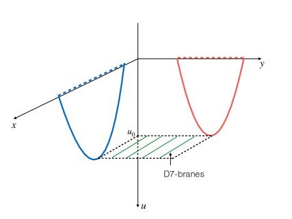
Figure 3: The configuration of the fundamental string and the $N_{\mathrm{D7}}$ D7-branes. The blue line refers to the case that the open string is put in $\left\{x,u\right\}$ plane i.e. parallel to the D7-branes. The red line refers to the case that the open string is put in $\left\{y,u\right\}$ plane i.e. vertical to the D7-branes. The D7-branes are represented by the green lines.

Taking the static gauge as $\tau=t\in\left[0,\mathcal{T}\right],\sigma=x\in\left[-\frac{R}{2},\frac{R}{2}\right],u=u\left(x\right)$, the Nambu-Goto action is given as,

$$S_{NG}^{\|} =-\frac{1}{2\pi\alpha^{\prime}}\int d\tau d\sigma\sqrt{-g_{\tau\tau}g_{\sigma\sigma}}$$

$$=-\frac{\mathcal{T}}{2\pi\alpha^{\prime}}\int dx\sqrt{-g_{00}\left[g_{xx}+g_{uu}u^{\prime}\left(x\right)^{2}\right]}$$

$$=-\frac{L^{2}\mathcal{T}}{2\pi\alpha^{\prime}}\int\frac{1}{u^{2}}\sqrt{1+\frac{u^{\prime 2}}{\mathcal{F}}}dx,$$ (3.19)

where the derivatives “ ^′ ” are with respect to $x$. Notice that the associated Hamiltonian to (3.19) is conserved i.e. a constant since the Lagrangian presented in (3.19) does not depend on $x$ explicitly. Accordingly we can reach

$$\mathcal{H} =u^{\prime}\frac{\partial\mathcal{L}}{\partial u^{\prime}}-\mathcal{L}$$

$$=\frac{L^{2}\mathcal{T}}{2\pi\alpha^{\prime}}\frac{1}{u^{2}\sqrt{1+\frac{u^{\prime 2}}{\mathcal{F}}}}=\frac{L^{2}\mathcal{T}}{2\pi\alpha^{\prime}}\times\mathrm{const}.$$ (3.20)

Imposing the condition $u^{\prime}\left(x\right)\big{|}_{u=u_{0}}=0$, the Hamiltonian reduces to

$$\frac{1}{u^{2}\sqrt{1+\frac{u^{\prime 2}}{\mathcal{F}}}}=\frac{1}{u_{0}^{2}},$$ (3.21)

which is equivalent to

$$\frac{du}{dx}=\sqrt{\mathcal{F}\left(\frac{u_{0}^{4}}{u^{4}}-1\right)}.$$ (3.22)

Plugging (3.22) into (3.19), the Nambu-Goto action is written as,

$$S_{NG}^{\|}=-\frac{L^{2}\mathcal{T}}{\pi\alpha^{\prime}}\int_{u_{0}}^{0}\frac{u_{0}^{2}}{u^{2}}\frac{du}{\sqrt{\mathcal{F}\left(u_{0}^{4}-u^{4}\right)}}.$$ (3.23)

So according to (3.16), the quark-antiquark potential can be obtained by subtracting (3.18) from (3.23) as,

$$V^{\|} =\frac{L^{2}\mathcal{T}}{\pi\alpha^{\prime}}\int_{u_{0}}^{0}\frac{1}{u^{2}\sqrt{\mathcal{F}}}\left[\frac{u_{0}^{2}}{\sqrt{\left(u_{0}^{4}-u^{4}\right)}}-1\right]$$

$$=\lambda^{1/2}M_{KK}\mathcal{C}\left(u_{0}\right)+\frac{a^{2}}{M_{KK}}\mathcal{C}^{\|}\left(u_{0}\right)+\mathcal{O}\left(a^{4}\right),$$ (3.24)

where we have used $V^{\|}$ to denote the quark potential with respect to the parallel case. The constants $\mathcal{C}\left(u_{0}\right)$ and $\mathcal{C}^{\|}\left(u_{0}\right)$ depending on $u_{0}$ have to be calculated numerically and their behaviors with respect to $u_{0}$ are given in Figure 4 .

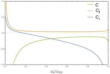
Figure 4: The numerical constants $\mathcal{C},\mathcal{C}_{\|},\mathcal{C}_{\bot}$ as functions of $u_{0}$.

Perpendicular to the D7-branes

The second situation is that the open string extends vertically to the D7-branes as it is illustrated in Figure 3. In this case we take the static gauge as $\tau=t\in\left[0,\mathcal{T}\right],\sigma=y\in\left[-\frac{R}{2},\frac{R}{2}\right],u=u\left(y\right)$, then the Nambu-Goto action is given as,

$$S_{NG}^{\bot} =-\frac{\mathcal{T}}{2\pi\alpha^{\prime}}\int dx\sqrt{-g_{00}\left[g_{yy}+g_{uu}u^{\prime}\left(y\right)^{2}\right]}$$

$$=-\frac{L^{2}\mathcal{T}}{2\pi\alpha^{\prime}}\int\frac{1}{u^{2}}\sqrt{\mathcal{H}+\frac{u^{\prime 2}}{\mathcal{F}}}dy,$$ (3.25)

where the derivatives “ ^′ ” are with respect to $y$. And the associated Hamiltonian to (3.25) reduces to a constant which is,

$$\frac{\mathcal{H}}{u^{2}\sqrt{\mathcal{H}+\frac{u^{\prime 2}}{\mathcal{F}}}}=\frac{\mathcal{H}_{0}}{u_{0}^{2}},$$ (3.26)

or equivalently

$$\frac{du}{dy}=\frac{\sqrt{\mathcal{F}\mathcal{H}}\sqrt{\mathcal{H}u_{0}^{4}-\mathcal{H}_{0}^{2}u^{4}}}{\mathcal{H}_{0}u^{2}}.$$ (3.27)

As the analysis in the parallel case, the quark-antiquark potential $V^{\bot}$ can be obtained by plugging (3.27) into (3.25) then subtracting (3.18). The final result is given as,

$$V^{\bot} =\frac{L^{2}\mathcal{T}}{2\pi\alpha^{\prime}}\int_{u_{0}}^{0}\frac{du}{u^{2}\sqrt{\mathcal{F}}}\left(\frac{u_{0}^{2}\sqrt{\mathcal{H}}}{\sqrt{\mathcal{H}u_{0}^{4}-\mathcal{H}_{0}^{2}u^{4}}}-1\right)$$

$$=\lambda^{1/2}M_{KK}\mathcal{C}\left(u_{0}\right)+\frac{a^{2}}{M_{KK}}\mathcal{C}^{\bot}\left(u_{0}\right)+\mathcal{O}\left(a^{4}\right),$$ (3.28)

where the constant $\mathcal{C}\left(u_{0}\right)$ and $\mathcal{C}^{\bot}\left(u_{0}\right)$ as functions of $u_{0}$ are given in Figure 4.

As we have required that the size of the compactified direction is sufficiently small $\delta z\rightarrow 0$, so that the functions $\mathcal{F},\mathcal{B},\phi$ in (2.6) are analytical. Thus the quark tension can be evaluated analytically. In the large $R$ limit, to minimize its energy, the fundamental string trends to stretch as much as possible over $u=u_{KK}$. According to (3.25), its effective tension would be proportional to $\sqrt{-g_{00}g_{xx,yy}}$ and the fundamental string would move approximately vertically up to UV cutoff around the extrema $x=\pm R/2$. Therefore in the large $R$ limit we can obtain

$$V^{\|,\bot}\simeq\frac{R}{2\pi\alpha^{\prime}}\sqrt{-g_{00}g_{xx,yy}}\big{|}_{u=u_{KK}}\equiv T_{s}^{\|,\bot}R,$$ (3.29)

which illustrates an area law of the Wilson loop. So the quark tension is evaluated as,

$$T_{s}^{\|} =\frac{1}{2\pi\alpha^{\prime}}\sqrt{-g_{00}g_{xx}}\big{|}_{u=u_{KK}}\simeq\frac{\lambda^{1/2}M_{KK}^{2}}{8\pi}-\frac{\log 32-2}{48\pi}\lambda^{1/2}a^{2}+\mathcal{O}\left(a^{4}\right),$$

$$T_{s}^{\bot} =\frac{1}{2\pi\alpha^{\prime}}\sqrt{-g_{00}g_{yy}}\big{|}_{u=u_{KK}}\simeq\frac{\lambda^{1/2}M_{KK}^{2}}{8\pi}-\frac{\log 4-2}{48\pi}\lambda^{1/2}a^{2}+\mathcal{O}\left(a^{4}\right).$$ (3.30)

As we can see the quark tension in the parallel case decreases while it increases in the perpendicular case. And this result is in agreement with our numerical calculation in the limit $u_{0}\rightarrow u_{KK}$. While it is not strictly to discuss the case that the anisotropy becomes large, the quark tension $T_{s}^{\|}$ could be vanished if $a$ increases, which may imply the deconfinement.

3.3 Entanglement entropy

Since the entanglement entropy is expected to be a probe to characterize the phase transition in the field theory, in this subsection let us compute the entanglement entropy in the anisotropic background (2.6).

We will take into account the region A and its complement, the region B, as two physically disjoint spatial regions in the dual theory. Based on the AdS/CFT correspondence [39, 52], in the dual theory the quantum entanglement entropy between region A and B is identified to be the surface $\gamma$ stretched in the bulk whose boundary coincides with the boundary of A. In general the classical area of surface $\gamma$ in the correspondence of AdS_d+2/CFT_d+1 is given as,

$$S_{\gamma}=\frac{1}{4G_{N}^{\left(d+2\right)}}\int_{\gamma}d^{d}x\sqrt{g_{\mathrm{ind}}},$$ (3.31)

where $G_{N}^{\left(d+2\right)}$ is the Newton constant in $d+2$ dimensional spacetime and $g_{\mathrm{ind}}$ is the induced metric on $\gamma$. In order to represent the entanglement entropy at a fixed time, surface $\gamma$ must be space-like. A natural generalization of (3.31) to the ten-dimensional geometry in string theory is

$$S_{\gamma}=\frac{1}{4G_{N}^{\left(10\right)}}\int_{\gamma}d^{8}xe^{-2\phi}\sqrt{g_{\mathrm{ind}}},$$ (3.32)

where the induced metric $g_{\mathrm{ind}}$ should be given in the string frame and the entanglement entropy can be obtained by minimizing the action (3.32). As the most simple case, we consider the “slab” geometry of A as $\mathbb{R}\times l$, however it would be straightforward to realize that the resultant entanglement entropy given by (3.32) depends on the configuration of the slab as we have seen in the cases of studying the Wilson loop, since the background metric (2.6) is anisotropic in the $\left\{x,y\right\}$ plane. Therefore let us proceed the calculations to obtain the entanglement entropy in two cases: parallel and perpendicular case, which is similar as what we have analyzed with the setup of Wilson loop in the previous section.

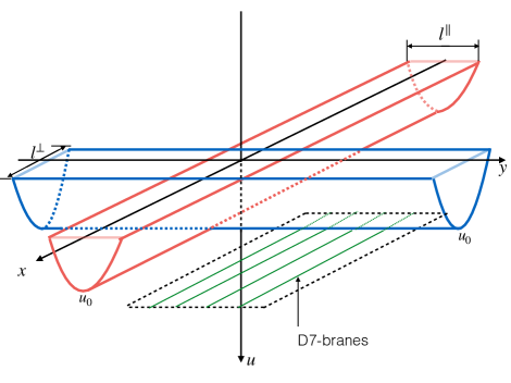
Figure 5: Surface stretched into the anisotropic bulk geometry. The red and blue case refers to that the slab is parallel and perpendicular to the D7-branes respectively. The D7-branes are denoted by the green lines.

Perpendicular case

Let us first deal with the case that the region A is perpendicular to the $N_{\mathrm{D7}}$ D7-branes as it is illustrated in Figure 5. The side of region $\gamma$ reduces to a curved line in $\left\{u,x\right\}$ plane, hence $u$ becomes a function of $x$ in the induced metric. Impose (2.6) into (3.32), after simple calculations we obtain the action of $\gamma$ as,

$$S^{\bot}=\frac{V}{4G}\int_{-\frac{l^{\bot}}{2}}^{\frac{l^{\bot}}{2}}dx\sqrt{h\left(u\right)}\sqrt{1+\beta u^{\prime 2}},$$ (3.33)

where the derivatives “ ^′ ” are with respect to $x$, $V$ refers to the infinity volume of the two-dimensional worldvolume and

$$\alpha\left(u\right)=\frac{L^{2}}{u^{2}},\beta\left(u\right)=\frac{1}{\mathcal{F}},h\left(u\right)=e^{-4\phi}V_{\mathrm{int}}^{2}\alpha\left(u\right)^{2},V_{\mathrm{int}}=2\pi^{4}R_{3}\frac{\mathcal{Z}^{5/2}L^{6}}{u}\sqrt{\mathcal{F}\mathcal{B}}.$$ (3.34)

The associated Hamiltonian to (3.33) must be a constant since the Lagrangian presented in (3.33) is independent on $x$. Thus it leads to,

$$\frac{du}{dx}=\frac{1}{\sqrt{\beta}}\sqrt{\frac{h\left(u\right)}{h\left(u_{0}\right)}-1},$$ (3.35)

i.e.

$$l^{\bot}\left(u_{0}\right)=2\sqrt{h\left(u_{0}\right)}\int_{0}^{u_{0}}\frac{du\sqrt{\beta\left(u\right)}}{\sqrt{h\left(u\right)-h\left(u_{0}\right)}},$$ (3.36)

where $l^{\bot}$ refers to the width of the region A. Obviously, the entanglement entropy given by (3.33) is divergent since it is proportional to the area of region A which therefore has to be renormalized. The “counterterm” can be obtained by evaluating the action of a surface extending along $u$. Afterwards, the finite entanglement entropy follows the formulas as,

$$\frac{2G}{V}\Delta S^{\bot}=\int_{0}^{u_{0}}du\sqrt{\beta h}\left(\frac{1}{\sqrt{1-\frac{h\left(u_{0}\right)}{h\left(u\right)}}}-1\right)-\int_{u_{0}}^{u_{KK}}du\sqrt{\beta h}.$$ (3.37)

By varying the value of $a$, the relation of $l^{\bot}$ and $u_{0}$, $\Delta S^{\bot}$ and $l^{\bot}$ is illustrated numerically in Figure 6 which displays the typical swallow-tail behavior with respect to $\Delta S^{\bot}$ and $l^{\bot}$.

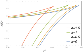
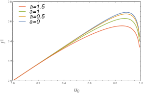
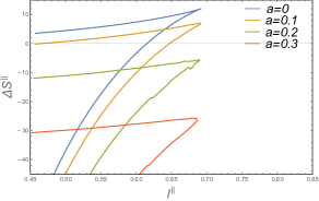
Figure 6: The behavior of width and entanglement entropy in perpendicular and parallel case. Upper: The relation of $l^{\bot}$ and $u_{0}$, $\Delta S^{\bot}$ and $l^{\bot}$ for perpendicular case. Lower: The relation of $l^{\|}$ and $u_{0}$, $\Delta S^{\|}$ and $l^{\|}$ for parallel case. We can see the typical swallow-tail behavior representing phase transition.

Notice that the critical value of $l^{\bot}$ , denoted by $l_{c}^{\bot}$ satisfying $\Delta S^{\bot}\left(l_{c}^{\bot}\right)=0$ decreases when $a$ increases. Although our numerical calculation may be exactly valid for small anisotropy, it implies the deconfinement phase transition may trend to be vanished when $a$ increases if the entanglement entropy does characterize the confinement as in [39, 40, 41, 42].

Parallel case

Let us turn to the case that the region A is parallel to the D7-branes as it is illustrated in Figure 5. Using (3.32), the action of $\gamma$ is given as,

$$S^{\|}=\frac{V}{4G}\int_{-\frac{l^{\|}}{2}}^{\frac{l^{\|}}{2}}dx\sqrt{h\left(u\right)}\sqrt{\mathcal{H}+\beta u^{\prime 2}},$$ (3.38)

where the derivatives “ ^′ ” are with respect to $y$. Then we can obtain the relation

$$\frac{du}{dy}=\sqrt{\frac{h\mathcal{H}^{2}-h_{0}\mathcal{H}_{0}\mathcal{H}}{h_{0}\mathcal{H}_{0}\beta}},$$ (3.39)

where $h_{0}=h\left(u_{0}\right),\mathcal{H}_{0}=\mathcal{H}\left(u_{0}\right)$ since the associated Hamiltonian is constant. Thus the the width $l^{\|}$ is given as,

$$l^{\|}\left(u_{0}\right)=2\sqrt{h_{0}}\int_{0}^{u_{0}}\frac{du\sqrt{\beta}}{\sqrt{h-h_{0}}}.$$ (3.40)

By subtracting the divergence in (3.38), the finite part of the entanglement entropy is given as,

$$\frac{2G}{V}\Delta S^{\|}=\int_{0}^{u_{0}}\sqrt{\beta H}\left(\frac{1}{\sqrt{\mathcal{H}-\frac{\mathcal{H}_{0}H_{0}}{\mathcal{H}H}}}-1\right)-\int_{u_{0}}^{u_{KK}}du\sqrt{\beta H}.$$ (3.41)

And the relation of $l^{\|}$ and $u_{0}$, $\Delta S^{\|}$ and $l^{\|}$ is also illustrated in Figure 6. While the numerical calculation shows the typical swallow-tail behavior with respect to $\Delta S^{\|}$ and $l^{\|}$, the associated phase transition trends to be vanished since there would not be a critical $l^{\|}$ satisfying $\Delta S^{\|}\left(l^{\|}\right)=0$ if anisotropy becomes sufficiently large. And again this conclusion is seemingly in agreement with the analysis of the Wilson loop if the entanglement entropy characterizes the confinement.

3.4 Baryon vertex

In the gauge-gravity duality, the baryon vertex is identified as a probe D-brane wrapped on the additional dimensions denoted by the spherical coordinates with $N_{c}$ open strings [43], and it can be treated as operator to create the baryon state. Accordingly, in the type IIB supergravity on $\mathrm{AdS}_{5}\times S^{5}$, the baryon vertex is a D5-brane wrapped on $S^{5}$.

To search for the stable wrapped configuration of D5-brane in the background (2.6), it would be straightforward to investigate the condition of the force balance for the baryon vertex. To begin with, let us decompose the metric on $\Omega_{5}$ by the coordinates of polar angle $\eta$ and $\Omega_{4}$, then define the radius coordinate $\xi$ as,

$$\frac{u_{KK}^{2}}{u^{2}}=\frac{1}{2}\left(\xi^{2}+\xi^{-2}\right).$$ (3.42)

Therefore the metric (2.6) becomes,

$$ds^{2}=\frac{L^{2}}{u^{2}}\left(-dt^{2}+dx^{2}+\mathcal{H}dy^{2}+\mathcal{F}\mathcal{B}dz^{2}\right)+\frac{L^{2}}{\xi^{2}}\mathcal{Y}d\xi^{2}+L^{2}\mathcal{Z}\left(d\eta^{2}+\sin^{2}\eta d\Omega_{4}^{2}\right),$$ (3.43)

where

$$\mathcal{Y}=\left(1-\frac{u^{4}}{u_{KK}^{4}}\right)\mathcal{F}^{-1},$$ (3.44)

which implies $\xi$ and $\eta$ refers respectively to the radius and polar angle in $\left\{\xi,\eta\right\}$ plane. Since the baryon vertex D5-brane extends along the directions of $\left\{t,\eta,\Omega_{4}\right\}$, the induced metric on a probe D5-brane is,

$$ds_{\mathrm{D5}}^{2}=-\frac{L^{2}}{u^{2}}dt^{2}+L^{2}\left(\mathcal{Y}\frac{\xi^{\prime 2}}{\xi^{2}}+\mathcal{Z}\right)d\eta^{2}+L^{2}\mathcal{Z}\sin^{2}\eta d\Omega_{4}^{2},$$ (3.45)

where the derivatives “ ^′ ” are with respect to $\eta$. To include the baryon potential, we turn on a single component of the gauge field on the D5-brane as $A=A_{t}\left(\eta\right)dt$, then the effective action for such a D5-brane is,

$$S_{\mathrm{D5}} =-T_{5}\int d^{6}xe^{-\phi}\sqrt{-\det\left(g_{\mathrm{D5}}+2\pi\alpha^{\prime}F\right)}-T_{5}\int A\wedge F_{5}\equiv-\frac{T_{5}V_{S^{4}}L^{6}}{\sqrt{2}u_{KK}}\int\mathcal{L}_{\mathrm{D5}}d\eta dt,$$ (3.46)

where $F=dA,T_{5}=\left(2\pi\right)^{-5}l_{s}^{-6}g_{s}^{-1}$ and

$$\mathcal{L}_{\mathrm{D5}} =\sin^{4}\eta\left[\sqrt{\left(\mathcal{Y}\xi^{\prime 2}+e^{\phi/2}\xi^{2}\right)\left(1+\xi^{-4}\right)-\tilde{F}_{t\eta}^{2}}-4\tilde{A}_{t}\right],$$

$$\tilde{A}_{t} =\frac{2\sqrt{2}\pi\alpha^{\prime}u_{KK}}{L^{2}}A_{t},\tilde{F}_{t\eta}=-\partial_{\eta}\tilde{A}_{t}.$$ (3.47)

Defining the displacement [44, 55],

$$D\left(\eta\right)=\frac{\partial\mathcal{L}_{\mathrm{D5}}}{\partial\tilde{F}_{t\eta}}=-\frac{\sin^{4}\eta\tilde{F}_{t\eta}}{\sqrt{\left(\mathcal{Y}\xi^{\prime 2}+e^{\phi/2}\xi^{2}\right)\left(1+\xi^{-4}\right)-\tilde{F}_{t\eta}^{2}}},$$ (3.48)

the equation of motion for $\tilde{A}_{t}$ can be written as,

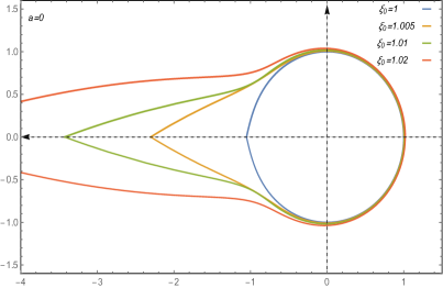
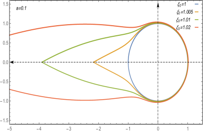
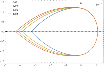
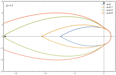
Figure 7: The configuration of the D5-brane as baryon vertex in $\left\{\xi,\eta\right\}$ plane. Note $\xi$ and $\eta$ is the radius and polar angle. In the upper figures, we fix $a=0,0.1$ respectively then adjust $\xi_{0}$; in the lower figures, we fix $\xi_{0}=1.1,1.2$ then adjust $a$. The numerical calculation always illustrates wrapped shape of the baryon vertex.

$$\partial_{\eta}D\left(\eta\right)=-4\sin^{4}\eta.$$ (3.49)

So the displacement is solved as,

$$D\left(\eta\right)=-\frac{3}{2}\eta+\frac{3}{2}\sin\eta\cos\eta+\sin^{3}\eta\cos\eta,$$ (3.50)

and the associated Hamiltonian to (3.47) is,

$$\mathcal{H}_{\mathrm{D5}} =\tilde{F}_{t\eta}\frac{\partial\mathcal{L}_{\mathrm{D5}}}{\partial\tilde{F}_{t\eta}}-\mathcal{L}_{\mathrm{D5}}$$

$$=-\sqrt{\left(\mathcal{Y}\xi^{\prime 2}+e^{\phi/2}\xi^{2}\right)\left(1+\xi^{-4}\right)}\sqrt{D^{2}\left(\eta\right)+\sin^{8}\eta}.$$ (3.51)

Accordingly the force at the cusp $U=U_{c}$ of D5-brane is given as,

$$F_{\mathrm{D5}}=-\frac{T_{5}V_{S^{4}}L^{6}}{\sqrt{2}u_{KK}}\int_{0}^{\pi}\frac{\partial\mathcal{H}_{\mathrm{D5}}}{\partial U_{c}}=N_{c}T_{F}\frac{\xi_{c}^{-4}+1}{\xi_{c}^{-4}-1}\frac{\mathcal{Y}_{c}\xi_{c}^{\prime}}{\sqrt{\mathcal{Y}_{c}\xi_{c}^{\prime 2}+e^{\phi_{c}}\xi_{c}^{2}}},$$ (3.52)

where $U=L^{2}/u$ is the standard radius coordinate of the bulk and we have used the index $c$ to refer to the value of the variables at $U=U_{c}$. For stable configuration located at $u_{c}=L^{2}/U_{c}$, the D5-brane must satisfy the zero-force condition i.e. $F_{\mathrm{D5}}=0$ if there is no other probe brane. It implies the zero-force condition can be achieved only if $\xi_{c}^{\prime}=0$ since $\mathcal{Y}$ is always positive in the bulk. Therefore the stable position for the baryon vertex in this system is located at $u_{c}\rightarrow u_{KK}$ to consistently minimize its action. To confirm our analysis, we also solve numerically the equation of motion associated to the Lagrangian presented in (3.47) to obtain the embedding function of the probe D5-brane. For a stable solution, we impose the boundary condition $\xi^{\prime}\left(0\right)=0,\xi\left(0\right)=\xi_{0}$ to the equation of motion, then the numerical solution for the configuration of the baryon vertex in $\left\{\xi,\eta\right\}$ plane is given in Figure 7. As we can see, there always exists wrapped solution for the baryon vertex and the configuration of $\xi_{0}=1$ is nearly independent on the variation of $a$. Thus the stable position for the D5-brane is indeed $u_{c}\rightarrow u_{KK}$ if the baryon vertex is the only probe brane.

To close this subsection, let us evaluate the baryon mass in this holographic system. Since the stable baryon vertex must be located at $u_{KK}$, its mass can be obtained by evaluate its onshell action (3.46) by setting $A=0$. Thus the Euclidean action of the D5-brane $S_{\mathrm{D5}}^{E}$ and baryon mass $m_{B}$ are identified via holography as,

$$S_{\mathrm{D5}}^{E}=T_{5}\int d^{6}xe^{-\phi}\sqrt{-\det g_{\mathrm{D5}}}\big{|}_{u=u_{KK}}=m_{B}\int dt.$$ (3.53)

Plugging the metric in (3.45) and the relation of $M_{KK},u_{KK}$ in (2.9) into (3.53), the baryon mass is evaluated as,

$$m_{B}=\frac{\lambda^{1/2}}{64\pi^{2}}M_{KK}N_{c}\left[1+\frac{\log 16-1}{6}\frac{a^{2}}{M_{KK}^{2}}+\mathcal{O}\left(a^{4}\right)\right],$$ (3.54)

which is enhanced in the presence of the Chern-Simons term represented by $a$. As we have specified in the Section 2, the dual theory is a topological massive theory due to the presence of the Chern-Simons term, so it would be easy to understand that baryon would also become topologically massive once the fundamental fermion is introduced. In addition, as the baryon mass is proportional to the worldvolume of the D5-brane (3.53), we find Figure 7 also illustrates the worldvolume is increased by the anisotropy which implies the increase of the baryon mass by the anisotropy.

4 Embedding of the D7-branes and the vacuum structure

In this section, we continue the holographic setup by introducing the various D7-branes to identify the dual field theory as QCD₃ in large $N_{c}$ limit. We first address the D7-branes as the flavor degrees of freedom then take into account another D7-brane in which the low-energy effective theory on its worldvolume is expected to be pure Chern-Simons theory. And we will see, the topological property in the dual theory can be studied by analyzing the configuration and orientation of these distinct D7-branes.

4.1 The flavor brane

As most works about the gauge-gravity duality, the fundamental matter can be added to the D3-brane background by embedding flavor D7-branes as probe. In our setup, we add $N_{f}$ coincident copies of D7-branes as probes to the D3-brane background (2.6), transverse to the compactified $z$ direction, spanning the $\mathbb{R}^{1,2}$ denoted by $\left\{t,x,y\right\}$, the holographic direction denoted by $u$ and four of the five directions in $\Omega_{5}$ as [45, 46]. The D-brane configuration including various D7-branes is illustrated in Table 3 where we have decomposed the directions of $\Omega_{5}$ as $\Omega_{4}$ and $w$.

Bubble background	$t$	$x$	$y$	$\left(z\right)$	$u$	$\Omega_{4}$	$w$
$N_{c}$ D3-branes	-	-	-	-
$N_{\mathrm{D7}}$ D7-branes	-	-		-		-	-
$N_{f}$ D7-branes	-	-	-		-	-
CS D7-branes	-	-	-			-	-

Table 3: The D-brane configuration including various D7-branes.

The leftover direction $w$ is transverse to both the $N_{c}$ color D3-branes and $N_{f}$ flavor D7-branes, so a bare mass for the flavors can be introduced by imposing a separation between color and flavor branes along $w$ direction at the UV boundary which breaks the parity in QCD₃. In the D3-D7 approach, the $w$ direction corresponding to the scalar in the D7-brane worldvolume couples to the mass operator of the fermions. And according to the gauge-gravity duality, the profile along the transverse direction of the flavor branes corresponds to the meson operator $\bar{\psi}\psi$ in the dual theory.

Then let us investigate the embedding of the flavor branes with their effective action. To specify the embedding of the flavor branes with respect to the transverse direction $w$, we first define a new radial coordinate $\rho$ as,

$$\frac{du^{2}}{u^{2}\mathcal{F}}=\frac{\mathcal{Z}}{\rho^{2}}d\rho^{2}.$$ (4.1)

Up to order of $\mathcal{O}\left(a^{2}\right)$, the relation of $u$ and $\rho$ can be solved as,

$$u\left(\rho\right)= u_{0}\left(\rho\right)+a^{2}u_{2}\left(\rho\right),$$

$$u_{0}\left(\rho\right)= \frac{2L^{2}u_{KK}^{2}\rho}{\sqrt{L^{8}+4u_{KK}^{4}\rho^{4}}},$$

$$u_{2}\left(\rho\right)= -\frac{L^{2}u_{KK}^{4}\rho}{24\left(L^{8}+4u_{KK}^{4}\rho^{4}\right)^{3/2}}\bigg{[}4L^{4}u_{KK}^{2}\rho^{2}+2L^{8}\left(\log 32-1\right)$$

$$-5\left(L^{8}+4u_{KK}^{4}\rho^{4}\right)\log\left(\frac{L^{8}+4u_{KK}^{2}\rho^{2}L^{4}+4u_{KK}^{4}\rho^{4}}{L^{8}+4u_{KK}^{4}\rho^{4}}\right)\bigg{]}.$$ (4.2)

We note that the ambiguity in this relation can be omitted by choosing $\rho^{2}\geq L^{4}/\left(u_{KK}^{2}2\right)$ for $a=0$. In this coordinate, the background metric (2.6) can be written as,

$$ds^{2}=\frac{L^{2}}{u^{2}}\left(-dt^{2}+dx^{2}+\mathcal{H}dy^{2}+\mathcal{F}\mathcal{B}dz^{2}\right)+\frac{L^{2}\mathcal{Z}}{\rho^{2}}\left(d\rho^{2}+\rho^{2}d\Omega_{5}^{2}\right),$$ (4.3)

where $u=u\left(\rho\right)$. Afterwards we impose the coordinate transformation $\zeta=\rho\cos\Theta,w=\rho\sin\Theta$ i.e. $\rho^{2}=w^{2}+\zeta^{2}$ where $\Theta$ is one angular coordinate in $\Omega_{5}$, then the metric (4.3) takes the final form as,

$$ds^{2}=\frac{L^{2}}{u^{2}}\left(-dt^{2}+dx^{2}+\mathcal{H}dy^{2}+\mathcal{F}\mathcal{B}dz^{2}\right)+\frac{L^{2}\mathcal{Z}}{\rho^{2}}\left(d\zeta^{2}+\zeta^{2}d\Omega_{4}^{2}+dw^{2}\right).$$ (4.4)

Since the flavor D7-branes extend along $\left\{t,x,y,u,\Omega_{4}\right\}$, the induced metric on the flavor branes is obtained as,

$$ds_{\mathrm{D7}}^{2}=\frac{L^{2}}{u^{2}}\left(-dt^{2}+dx^{2}+\mathcal{H}dy^{2}\right)+\frac{L^{2}\mathcal{Z}}{\rho^{2}}\left[\left(w^{\prime 2}+1\right)d\zeta^{2}+\zeta^{2}d\Omega_{4}^{2}\right],$$ (4.5)

where $w=w\left(\zeta\right)$ and the derivatives “ ^′ ” are with respect to $\zeta$. So the action for a single flavor D7-brane is,

$$S_{\mathrm{D7}} =-T_{7}\int d^{8}xe^{-\phi}\sqrt{-g_{\mathrm{D7}}}=-T_{7}V_{3}V_{S^{4}}L^{8}\int d\zeta\mathcal{L},$$

$$\mathcal{L} =\frac{e^{-\phi/4}\zeta^{4}\sqrt{1+w^{\prime 2}}}{u^{3}\rho^{5}}.$$ (4.6)

The behavior of the embedding function of the flavor D7-branes can be obtained by solving the associated equation of motion to the action in (4.6), which is,

$$\frac{\partial}{\partial\zeta}\left[\frac{e^{-\phi/4}\zeta^{4}w^{\prime}}{u\left(\rho\right)^{3}\rho^{5}\sqrt{1+w^{\prime 2}}}\right]-\frac{\partial}{\partial w}\left[\frac{e^{-\phi/4}\zeta^{4}\sqrt{1+w^{\prime 2}}}{u\left(\rho\right)^{3}\rho^{5}}\right]=0.$$ (4.7)

Since a parity transformation acts as $w\left(\zeta\right)\rightarrow-w\left(\zeta\right)$, for the massless case, we have to impose the boundary condition

$$w^{\prime}\left(\zeta\right)\bigg{|}_{\zeta=0}=0,w\left(\zeta\right)\bigg{|}_{\zeta=\infty}=0.$$ (4.8)

Keeping these in hand, we numerically solve the equation of motion (4.7) with various $a$ in the region $\zeta>0$ which is illustrated in Figure 8.

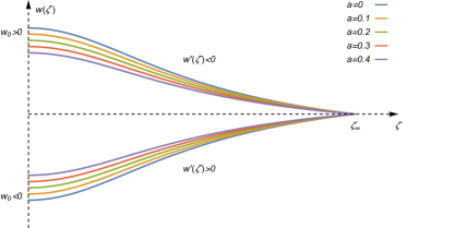
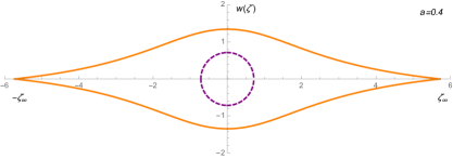
Figure 8: The two parity-related minimal embeddings of the flavor branes in the massless case with various $a$. The parameter is chosen as $L^{2}/u_{KK}=1,\zeta_{\infty}=5.73$. Upper: the dependence on $a$ of the flavor embeddings. Lower: the full configuration of the parity-related flavor branes with a fixed $a$. The purple dashed line represents the position $u=u_{KK}$.

The numerical calculation shows a very small shift with respect to the dependence on $a$ (we have enlarged the shift in the figure) and this behavior is opposite to the approach of the D3-D(-1) background [45]. We note here the two branches of the flavor branes trend to become coincident if $a$ increases. The full configuration of the embedding D7-branes is given in Figure 8 and we also calculate the massive case by setting the boundary condition $w_{\infty}\neq 0$ in Figure 9.

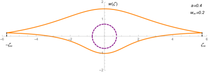
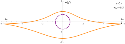
Figure 9: The massive case of the embedding flavor branes with fixed $a$. Upper: the positive mass case with $w_{\infty}=0.2$. Lower: the negative mass case with $w_{\infty}=-0.2$.

Note that the number of the node in the embedding function refers to the excitation of the D-brane configuration. For a vacuum configuration, we only take the non-node solution as it is shown in Figure 8 and Figure 9 which means equivalently the node is located at $\zeta=\infty$.

4.2 The Chern-Simons brane

Due to the presence of the axion field $\chi$ in the bulk, the D3-D7 brane background (2.6) corresponds to the QCD₃ with a Chern-Simons term in holography. Thus the present $N_{\mathrm{D7}}$ D7-branes should contribute to some vacuum properties of the dual theory. However, once we evaluate the embedding function of such a D7-brane as probe, its equation of motion implies the only solution for $u=u_{KK}$ and its onshell action automatically vanishes. To include the set-up of a pure Chern-Simons theory, we follow the discussion in the D3-brane approach [46], to introduce $k_{b}$ coincident Chern-Simons (CS) as probe D7-branes where the configuration is given in Table 3. At very low energies, all other excitations on the Chern-Simons branes decouple and only a Wess-Zumino term is left as,

$$S_{WZ}=\frac{1}{2\left(2\pi\right)^{5}l_{s}^{4}}\int C_{4}\wedge\mathrm{Tr}\left(F\wedge F\right)=-\frac{1}{2\left(2\pi\right)^{5}l_{s}^{4}}\int_{S^{5}}F_{5}\int_{\mathbb{R}^{2+1}}\omega_{3}=-\frac{N_{c}}{4\pi}\int_{\mathbb{R}^{2+1}}\omega_{3}.$$ (4.9)

Therefore we can see the gauge-gravity duality in this setup reduces to the well-known level/rank duality $SU\left(N_{c}\right)_{k_{b}}\leftrightarrow U\left(k_{b}\right)_{-N_{c}}$ in quantum field theory (QFT) expectations precisely [45, 46, 56].

To obtain the embedding of the Chern-Simons brane, we need to evaluate the equation of motion by its effective action. Recall the induced metric on a D7-brane (4.5), the action for Chern-Simons brane takes the same formula as given in (4.6), thus its associated equation of motion is given in (4.7) while $\rho$ must be a constant for a Chern-Simons brane. Accordingly, we impose the following ansatz

$$w\left(\zeta\right)=\sqrt{\frac{L^{4}}{2u_{KK}^{2}}\kappa-\zeta^{2}},$$ (4.10)

to the equation of motion of $w\left(\zeta\right)$ which reduces to a constraint for $\kappa$ and $a$ as,

$$0= -48\left(\kappa^{5}+\kappa^{4}-\kappa-1\right)+a^{2}\bigg{[}-6+30\log 2+\kappa\big{(}12-16\kappa+12\kappa^{2}-18\kappa^{3}$$

$$+\left(6+2\kappa+2\kappa^{2}\right)\log 32\big{)}+12\left(\kappa^{5}+\kappa^{4}-\kappa-1\right)\log\left(1+\frac{2\kappa}{1+\kappa^{2}}\right)\bigg{]},$$ (4.11)

where we have set $L^{2}/u_{KK}=1$. And this constraint can be solved numerically as it is illustrated in Figure 10.

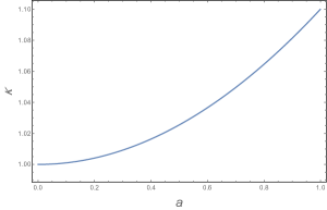
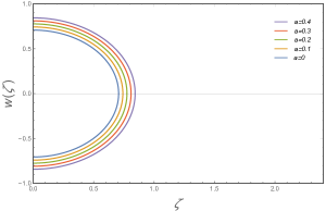
Figure 10: Left:The relation of $\kappa$ and $a$. Right: The embedding of the Chern-Simons brane on $\left\{w,\zeta\right\}$ plane.

The numerical calculation also illustrates a very small shift with respect to the dependence on $a$ for the embedding of the Chern-Simons brane. Then the ground energy of the Chern-Simons brane can be evaluated by its action as

$$S_{\mathrm{D7}}^{\mathrm{CS}}=-T_{7}\int d^{8}xe^{-\phi}\sqrt{-g_{\mathrm{D7}}}=-T_{7}V_{3}V_{S^{5}}L^{8}e^{-\frac{\phi}{4}}u^{-3}.$$ (4.12)

The action is minimized at $u=u_{KK}$, so we can obtain the ground energy density $E_{\mathrm{CS}}$ of the Chern-Simons brane is obtained by

$$E_{\mathrm{CS}}=-\frac{S_{\mathrm{D7}}^{\mathrm{CS}}}{V_{3}}=T_{7}V_{S^{5}}L^{8}u_{KK}^{-3}\left(1+\frac{\log 2}{16}a^{2}u_{KK}^{2}\right)+\mathcal{O}\left(a^{4}\right).$$ (4.13)

5 The phase diagram involving the massive flavors

In the previous sections, we have evaluated the embedding of the Chern-Simons and flavor branes with massless boundary condition. Here we are going to study the configurations having both Chern-Simons and flavor branes with massive boundary condition since the vacuum of QCD₃ with Chern-Simons term would include both of them in general. Then the phase diagram would be obtained by evaluating the energies of these D7-branes.

5.1 The energy of massive embedding flavor brane

In order to obtain the energy of the flavor branes with massive boundary condition, let us take a look at the asymptotic behavior of the embedding functions which satisfies the equation of motion (4.7), although the embedding configuration of the flavor branes has been illustrated in Figure 9. Since the flavor mass corresponds to the boundary value of $w\left(\zeta\right)$, we can find the asymptotics of (4.7) at $\zeta\rightarrow\infty$ ($\rho\rightarrow\zeta$) as,

$$\frac{d}{d\zeta}\left(\zeta^{2}w^{\prime}\right)=-2w,$$ (5.1)

where the relation (4.2) and boundary behavior of $\phi$ have been imposed. For massless case, the general form of the asymptotics at large $\zeta$ for $w\left(\zeta\right)$ would be,

$$w\left(\zeta\right)=\pm\sqrt{\frac{\mu^{3}}{\zeta}}\sin\left(\frac{\sqrt{7}}{2}\log\frac{\zeta}{\zeta_{\infty}}\right),$$ (5.2)

where $\mu$ is a constant energy scale. So a simple way to obtain the asymptotics at large $\zeta$ with massive boundary condition is to consider a very small variation of $w$,

$$\delta w_{\infty}=\sqrt{\frac{\mu}{\zeta_{\infty}}}2\pi l_{s}^{2}\delta m,$$ (5.3)

due to

$$\lim_{\zeta\rightarrow\infty}w\left(\zeta\right)\rightarrow\frac{1}{\sqrt{\zeta}}.$$ (5.4)

Keeping these in hand, then let us investigate the associated variation in the on-shell action of the flavor brane which is given by recalling (4.6) (4.7)

$$\delta S_{\mathrm{D7}} =\frac{\partial\mathcal{L}}{\partial w^{\prime}}\delta w\bigg{|}_{\zeta=0}^{\zeta=\zeta_{\infty}}=-T_{7}V_{3}V_{S^{4}}L^{8}\left[\frac{e^{-\phi/4}\zeta^{4}w^{\prime}}{u\left(\rho\right)^{3}\rho^{5}\sqrt{1+w^{\prime 2}}}\delta w\right]\bigg{|}_{\zeta=0}^{\zeta=\zeta_{\infty}}.$$ (5.5)

Notice the relation of the flavor brane energy $E_{f}$ and on-shell action is $E_{f}=-\frac{S_{\mathrm{D7}}}{V_{3}}$, using (5.5), the contribution of the massive part to the flavor brane energy (density) is evaluated as,

$$\delta E_{f} =T_{7}V_{S^{4}}L^{2}\frac{e^{-\phi\left(\zeta_{\infty}\right)/4}\zeta^{2}w^{\prime}\left(\zeta_{\infty}\right)}{\sqrt{1+w^{\prime 2}\left(\zeta_{\infty}\right)}}\delta w_{\infty}=\mp c\delta m,$$

$$c =e^{-\phi\left(\zeta_{\infty}\right)/4}\frac{N_{c}\sqrt{g_{s}N_{c}}}{24\pi^{5/2}}M_{\mu}^{2},$$ (5.6)

where we have introduced a energy scale $M_{\mu}=2\mu/L^{2}$ and “$\mp$” corresponds to the negative/positive mass of the flavor as it is illustrated in Figure 9. Afterwards, the total energy of flavor brane $E_{f}\left(m\right)$ with massive boundary condition can be obtained by its massless part of energy $E_{f}\left(0\right)$ plus the massive contribution $\delta E_{f}$ as,

$$E_{f}\left(m\right)=E_{f}\left(0\right)+\delta E_{f}.$$ (5.7)

Thus the flavor condensate in this system can be obtained as,

$$\left\langle\bar{\psi}\psi\right\rangle=\frac{dE_{f}\left(m\right)}{dm}=\pm c,$$ (5.8)

for positive/negative mass.

To close this subsection, let us evaluated the total energy of the D-brane configuration that $p$ of $N_{f}$ flavor branes extend in the upper $\left\{w,\zeta\right\}$ plane while the other $N_{f}-p$ flavor branes extend in the lower $\left\{w,\zeta\right\}$ plane, as it is illustrated in Figure 11. Since the energy of each flavor brane should be equivalent, for the massless case, the total energy is given by

$$E_{f}^{tot}\left(0\right)=pE_{f}\left(0\right)+\left(N_{f}-p\right)E_{f}\left(0\right)=N_{f}E_{f}\left(0\right).$$ (5.9)

Then for the massive case, suppose the $N_{f}$ flavor branes have a common mass $m$, the degeneracy between the flavor branes extending in upper and down lower $\left\{w,\zeta\right\}$ plane is lifted for $m\neq 0$, therefore we could get the total energy as,

$$E_{f}^{tot}\left(m\right) =p\left[E_{f}\left(0\right)-cm\right]+\left(N_{f}-p\right)\left[E_{f}\left(0\right)+cm\right]$$

$$=N_{f}E_{f}\left(0\right)-\left(N_{f}-2p\right)cm.$$ (5.10)

We note that this formula of the total energy in this D-brane configuration would be useful to study the various phase in the dual theory.

5.2 The topological phase

In order to identify the vacuum structure of the D7-branes with the various phases in the dual theory, we need to give a well-defined Chern-Simons level in which the Chern-Simons level depends on the number of the flavor branes. The details to obtain this goal have been discussed in [45, 46], so let us briefly outline the main idea and investigate the phase transition in our holographic setup.

First the effective Chern-Simons level $k_{eff}$ according to the holographic duality is given as,

$$\int_{S^{1}}F_{1}=-k_{eff},$$ (5.11)

where $S^{1}$ is a circle whose location is among all other coordinates except $\left\{w,\zeta\right\}$. Thus it is a fixed point in the $\left\{w,\zeta\right\}$ plane. Then we define the “$p$ sector”, that is a D-brane configuration with $p$ flavor branes extending in the upper $\left\{w,\zeta\right\}$ plane and $N_{f}-p$ flavor branes extending in the lower plane. Afterwards, we take into account the contribution to $k_{eff}$ by counting the number of the orientation in the $\left\{w,\zeta\right\}$ plane of the D7-branes. For instance, the contribution to the effective Chern-Simons number $k_{eff}$ of D7-branes with counterclockwise/clockwise orientation in the $\left\{w,\zeta\right\}$ plane is positive/negative respectively, as it is illustrated in Figure 11 (while we show the massless case, it would be same for the massive case.).

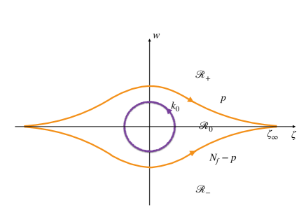
Figure 11: The D-brane configuration including Chern-Simons (purple) and flavor (orange) branes in the $\left\{w,\zeta\right\}$ plane with massless boundary condition. $p$ of $N_{f}$ flavor branes extend in the upper plane while the other $N_{f}-p$ flavor branes extend in the lower plane. The Chern-Simons is located at $u=u_{KK}$ to minimize its energy as discussed in Section 4.2.

Therefore the effective Chern-Simons level $k_{eff}$ with respected to the orientation reads,

$$k_{eff}=\begin{cases}k_{0}-p,&\mathrm{in}\ \mathcal{R}_{+},\\ k_{0},&\mathrm{in}\ \mathcal{R}_{0},\\ k_{0}+N_{f}-p,&\mathrm{in}\ \mathcal{R}_{-},\end{cases}$$ (5.12)

where $k_{0}$ is the number of the Chern-Simons branes which is given as $k_{0}=k+p-\frac{N_{f}}{2},k\in\mathbb{Z}$ since both branches of flavor branes at the intersection point count one-half i.e. $k_{eff}=k_{0}-p+\frac{N_{f}}{2}$.

At low energy, the interpretation of such a D-brane configuration in holography is that the flavor symmetry $U\left(N_{f}\right)$ spontaneously breaks down to $U\left(p\right)\times U\left(N_{f}-p\right)$. So $2p\left(N_{f}-p\right)$ Goldstone bosons are created and the associated target space is Grassmann,

$$\mathrm{Gr}\left(p,N_{f}\right)=\frac{U\left(N_{f}\right)}{U\left(p\right)\times U\left(N_{f}-p\right)}.$$ (5.13)

On the other hand, since the presence of the Chern-Simons leads to a level/rank duality $U\left(\left|k+p-\frac{N_{f}}{2}\right|\right)_{N}\leftrightarrow SU\left(N\right)_{k+p-N_{f}/2}$, the dynamics of a $p$ sector at low-energy takes the symmetry,

$$\mathrm{Gr}\left(p,N_{f}\right)\times SU\left(N\right)_{k+p-N_{f}/2},$$ (5.14)

in which the vacuum of the dual theory is described by the $N_{f}+1$ sectors via holography. Afterwards, we can investigate the phase diagram by evaluating the total energy including both flavor and Chern-Simons branes. Recall (4.13) and (5.10), the total energy including flavor and Chern-Simons branes is collected as,

$$E_{\mathrm{vac}}\left(a\right) =E_{f}^{tot}\left(m\right)+k_{0}E_{\mathrm{CS}}$$

$$=N_{f}E_{f}\left(0\right)-\left(N_{f}-2p\right)cm+\left(k+p-\frac{N_{f}}{2}\right)E_{\mathrm{CS}}.$$ (5.15)

The phase diagram can be obtained by minimizing the energy $E_{\mathrm{vac}}\left(a\right)$ in (5.15). To find the dependence on the anisotropy (denoted by $a$), we require that the value of $a$ is fixed when we minimize $E_{\mathrm{vac}}\left(a\right)$. Then the results are collected as, for $k>N_{f}/2$,

$$E_{\mathrm{vac}}=\begin{cases}\left(k-N_{f}/2\right)E_{\mathrm{CS}},&m<m^{*},\ \ \ \ SU\left(N_{c}\right)_{k-N_{f}/2},\\ \left(k+N_{f}/2\right)E_{\mathrm{CS}}-2N_{f}cm,&m>m^{*},\ \ \ \ SU\left(N_{c}\right)_{k+N_{f}/2},\end{cases}$$ (5.16)

where $SU\left(N_{c}\right)_{k\pm N_{f}/2}$ refers to the symmetry group of the corresponding topological phase. And for $k<N_{f}/2$, the associated topological phase and free energy are collected as,

$$E_{\mathrm{vac}}=\begin{cases}\left(N_{f}/2-k\right)E_{\mathrm{CS}},&\ \ \ m<-m^{*},\ \ \ \ \ \ \ SU\left(N_{c}\right)_{k-N_{f}/2},\\ 2\left(k-N_{f}/2\right)cm,&-m^{*}<m<m^{*},\ \ \ \ \ \ \ \mathrm{Gr}\left(p,N_{f}\right),\\ \left(N_{f}/2+k\right)E_{\mathrm{CS}}-2N_{f}cm,&\ \ \ \ m>m^{*},\ \ \ \ \ \ \ \ SU\left(N_{c}\right)_{k+N_{f}/2},\end{cases}$$ (5.17)

where $m^{*}$ refers to the critical value of the mass when the phase transition occurs, given as,

$$m^{*}=\frac{E_{\mathrm{CS}}}{2c}=\frac{3}{16}\frac{\lambda^{1/2}\pi^{1/2}M_{KK}^{3}}{M_{\mu}^{2}}\left(1+\frac{2-\log 16}{4}\frac{a^{2}}{M_{KK}^{2}}\right)+\mathcal{O}\left(a^{4}\right).$$ (5.18)

Here a noteworthy feature is that the critical mass may become vanished if the axion field or the anisotropy in the bulk becomes very non-negligible i.e $a$ becomes sufficiently large. In this sense the Grassmann phase $\mathrm{Gr}\left(p,N_{f}\right)$ would not exist which seemingly means the broken flavor symmetry is restored. Although our setup may be exactly valid only for small anisotropy, this result is instructively suggestive to study the anisotropic behavior of the metastable vacua in QCD₃ via holography.

6 Summary and discussion

In this work, we construct the anisotropic black D3-brane solution in IIB supergravity [12] then obtain the anisotropic bubble configuration for QCD₃ with a Chern-Simons term due to the presence of the axion field. The analytical formulas for the the background geometry is available since the dual theory is exactly three-dimensional theory in the compactification limit, as it is expected. With this analytical bulk geometry, we investigate the ground-state energy density, quark potential, entanglement entropy and baryon vertex in the dual theory according to the AdS/CFT dictionary. Technically, we consider small anisotropy to avoid the difficulty in our numerical calculation. Then all the results show the dependence of the axion field or the anisotropy in bulk as it is expected. Afterwards we introduce various probe D7-branes as flavor and Chern-Simons branes to include flavor matters and topological numbers in the dual theory. By examining the embedding functions and counting the orientation of these D7-branes, we obtain the vacuum energy associated to the corresponding effective Chern-Simons level, hence the phase transition can be achieved by comparing the various vacuum energies.

To close this work, let us give some comments about this project. Due to the presence of the axion in bulk, the quark potential and entanglement entropy are shifted as some holographic studies in four-dimensional QCD with an axion e.g. [23, 26]. However our work additionally implies the quark tension and the potential phase transition illustrated in the behavior of the entanglement entropy could be destroyed in the presence of strong anisotropy. These can be found in Section 3.2 and Section 3.3: when the anisotropy increases, we can see the quark tension trends to become vanished and there would not be a critical value of $l^{\perp,||}$ satisfying the entanglement entropy $\Delta S^{\perp,||}=0$. As the entanglement entropy could be a tool to characterize the confinement [39, 40, 41, 42], this behavior implies there would be no phase transition for $a\gg 1$ i.e. no confinement for strong anisotropy. Besides, the baryon vertex also reveals the unwrapped trend when the anisotropy becomes large and the “unwrapped baryon vertex” also means deconfinement [44]. In a word, this holographic approach shows us the confinement can not maintain in an extremely anisotropic situation. Interestingly, this conclusion is in agreement with the fact that the QGP is anisotropic and deconfined, so it may provide a holographic way to understand the features of the strongly coupled matter with anisotropy.

On the other hand, the dependence on the axion or the anisotropy of the critical mass in the topological phase transition would also be a parallel computation to the D3-(D-1) approach [45] and the extension of [46] by including an dynamical axion field. Moreover, as the critical mass trends to be vanished when the anisotropy increases, it means the Grassmann target space would not exist. Namely the broken flavor symmetry would be restored if the anisotropy becomes sufficiently large. We note that this behavior is also illustrated in Figure 8. As we can see in Figure 8 the flavor branes in the upper and lower branches trend to be coincident if $a$ increases greatly, i.e. the flavor symmetry $U\left(p\right)\times U\left(N_{f}-p\right)$ would be restored to $U\left(N_{f}\right)$ if $a\rightarrow\infty$. Accordingly, this behavior implies the flavor symmetry, which is related to the chiral symmetry, would be restored when the anisotropy is extremely strong.

Combine the above together, this holographic system reveals a potential conclusion that is the confinement will not maintain and the flavor symmetry (or probably chiral symmetry) would be restored in an extremely anisotropic situation. This conclusion adheres to intuition, because if the anisotropy becomes very large for a fixed $M_{KK}$ as $a\gg M_{KK}$, the dual theory depending on $a$ would include modes above the scale $M_{KK}$ thus the dual theory is decompactified and non-confining according to [38, 39]. Remarkably, all the analyses are exactly coincident with the characteristic properties of QGP, particularly it is usually to be treated as the fundamental assumption to study the deconfined matter in holography [57, 58, 59, 60]. Therefore, while we can only work out numerically the case that the anisotropy is small in this project, our framework would be very instructive to study QCD and Chern-Simons theory with anisotropy.

Appendix: The analytical formulas for the anisotropic background

In the high temperature limit $T\rightarrow\infty$, $\delta t_{E}\rightarrow 0$. The functions $\mathcal{F},\mathcal{B},\phi$ presented in the anisotropic black brane background (2.2) can be written as a series of $a$ up to $\mathcal{O}\left(a^{2}\right)$ as [12],

$$\mathcal{F}\left(u\right) =1-\frac{u^{4}}{u_{H}^{4}}+a^{2}\hat{\mathcal{F}}_{2}\left(u\right)+\mathcal{O}\left(a^{4}\right),$$

$$\mathcal{B}\left(u\right) =1+a^{2}\hat{\mathcal{B}}_{2}\left(u\right)+\mathcal{O}\left(a^{4}\right),$$

$$\phi\left(u\right) =a^{2}\hat{\phi}_{2}\left(u\right)+\mathcal{O}\left(a^{4}\right),$$ (A-1)

where

$$\hat{\mathcal{F}}_{2}\left(u\right) =\frac{1}{24u_{H}^{2}}\left[8u^{2}\left(u_{H}^{2}-u^{2}\right)-10u^{4}\log 2+\left(3u_{H}^{4}+7u^{4}\right)\log\left(1+\frac{u^{2}}{u_{H}^{2}}\right)\right],$$

$$\hat{\mathcal{B}}_{2}\left(u\right) =-\frac{u_{H}^{2}}{24}\left[\frac{10u^{2}}{u_{H}^{2}+u^{2}}+\log\left(1+\frac{u^{2}}{u_{H}^{2}}\right)\right],$$

$$\hat{\phi}_{2}\left(u\right) =-\frac{u_{H}^{2}}{4}\log\left(1+\frac{u^{2}}{u_{H}^{2}}\right).$$ (A-2)

We note that (A-1) and (A-2) is in fact a series of $u_{H}a$ (or equivalently $a/T$), so the high temperature limit exactly refers to the case $T\gg a$ in [12] which corresponds to $u_{H}a\ll 1$ or $a/T\ll 1$ in (A-1) (A-2). In the black brane background (2.2), $u_{H}$ refers to the horizon. In the bubble background (2.6), the double wick rotation reduces to the replacement $T\rightarrow M_{KK}/\left(2\pi\right),\delta t_{E}\rightarrow\delta z$ in the black brane solution. Note that $u_{H}$ is replaced by $u_{KK}$ in the bubble background (2.6) since $u_{KK}$ refers to the bottom of the bulk instead of a horizon as it is illustrated in Figure 1. And the formulas of $\mathcal{F},\mathcal{B},\phi$ remain while we replace $u_{H}$ by $u_{KK}$. Clearly the high temperature limit in the black brane solution corresponds to the limit of dimension reduction in the bubble solution i.e. the limit for that the compactified direction $z$ shrinks to zero in (2.6) i.e. $\delta z\rightarrow 0$, or equivalently $M_{KK}\rightarrow\infty$.

On the other hand, the dual theory on the $N_{c}$ D3-branes in the bubble background (2.6) is effectively three-dimensional below the energy scale $M_{KK}$. So if we take $M_{KK}\rightarrow\infty$, the dual theory would become exactly three-dimensional theory. Therefore, the analytical formulas (A-1) (A-2) for functions $\mathcal{F},\mathcal{B},\phi$ can always be employed by replacing $u_{H}\rightarrow u_{KK}$ in the bubble background (2.6) since the dual theory is always expected to be exactly three-dimensional theory, which means $M_{KK}\rightarrow\infty$ is always expected even if $a$ becomes large but fixed. In a word, using (A-1) (A-2) in the bubble background means the dual theory is exactly three-dimensional theory. In this sense, we believe our analysis in this work with (A-1) (A-2) is also valid for large $a$ under $M_{KK}\rightarrow\infty$.

References

- [1] O. Aharony, S. S. Gubser, J. M. Maldacena, H. Ooguri and Y. Oz, “Large N field theories, string theory and gravity”, Phys. Rept. 323 (2000) 183, arXiv:hep-th/9905111.
- [2] E. Witten, “Anti-de Sitter space and holography”, Adv.Theor.Math.Phys. 2 (1998) 253-291, arXiv:hep-th/9802150.
- [3] E. Shuryak, “Why does the quark gluon plasma at RHIC behave as a nearly ideal fluid?”, Prog.Part.Nucl.Phys. 53 (2004) 273-303, arXiv:hep-ph/0312227.
- [4] E. Shuryak, “What RHIC experiments and theory tell us about properties of quark-gluon plasma? ”, Nucl.Phys.A 750 (2005) 64-83, arXiv:hep-ph/0405066.
- [5] W. Florkowski, R. Ryblewski, “Highly-anisotropic and strongly-dissipative hydrodynamics for early stages of relativistic heavy-ion collisions”, Phys.Rev.C 83 (2011) 034907, arXiv:1007.0130.
- [6] R. Ryblewski, W. Florkowski, “Non-boost-invariant motion of dissipative and highly anisotropic fluid”, J.Phys.G 38 (2011) 015104, arXiv:1007.4662.
- [7] M. Martinez, M. Strickland, “Dissipative Dynamics of Highly Anisotropic Systems”, Nucl.Phys.A 848 (2010) 183-197, arXiv:1007.0889.
- [8] M. Martinez, M. Strickland, “Non-boost-invariant anisotropic dynamics”, Nucl.Phys.A 856 (2011) 68-87, arXiv:1011.3056.
- [9] D. Giataganas, U. Gürsoy, J. Pedraza, “Strongly-coupled anisotropic gauge theories and holography”, Phys.Rev.Lett. 121 (2018) 12, 121601, arXiv:1708.05691.
- [10] E. Banks, “Phase transitions of an anisotropic N=4 super Yang-Mills plasma via holography”, JHEP 07 (2016) 085, arXiv:1604.03552.
- [11] D. Ávila, D. Fernández, L. Patiño, D. Trancanelli, “Thermodynamics of anisotropic branes”, JHEP 11 (2016) 132, arXiv:1609.02167.
- [12] D. Mateos, D. Trancanelli, “Thermodynamics and Instabilities of a Strongly Coupled Anisotropic Plasma”, JHEP 07 (2011) 054, arXiv:1106.1637.
- [13] A. Rebhan, D. Steineder, “Violation of the Holographic Viscosity Bound in a Strongly Coupled Anisotropic Plasma”, Phys.Rev.Lett. 108 (2012) 021601, arXiv:1110.6825.
- [14] D. Mateos, D. Trancanelli, “The anisotropic N=4 super Yang-Mills plasma and its instabilities”, Phys.Rev.Lett. 107 (2011) 101601, arXiv:1105.3472.
- [15] E. Vicari, H. Panagopoulos, “Theta dependence of SU(N) gauge theories in the presence of a topological term”, Phys. Rept. 470, 93 (2009), arXiv:0803.1593.
- [16] M. D’Elia, F. Negro, “Theta dependence of the deconfinement temperature in Yang-Mills theories”, PhysRevLett.109.07200, arXiv:1205.0538.
- [17] M. D’Elia, F. Negro, “Phase diagram of Yang-Mills theories in the presence of a theta term”, Phys. Rev. D 88, 034503 (2013), arXiv:1306.2919.
- [18] L.Debbio, G. Manca, H. Panagopoulos, A. Skouroupathis, E. Vicari, “Theta-dependence of the spectrum of SU(N) gauge theories”, JHEP 0606:005,2006, [arXiv:hep-th/0603041].
- [19] D. Kharzeev, R.D. Pisarski, M. H. G. Tytgat, “Possibility of spontaneous parity violation in hot QCD”, Phys.Rev.Lett. 81 (1998) 512-515, arXiv:hep-ph/9804221.
- [20] K. Buckley, T. Fugleberg, A. Zhitnitsky, “Can theta vacua be created in heavy ion collisions?”, Phys.Rev.Lett. 84 (2000) 4814-4817, arXiv:hep-ph/9910229.
- [21] K. Fukushima, D. Kharzeev, H. Warringa, “The Chiral Magnetic Effect”, PhysRevD.78.074033, arXiv:0808.3382.
- [22] D. Kharzeev, “The Chiral Magnetic Effect and Anomaly-Induced Transport”, j.ppnp.2014.01.002, arXiv:1312.3348.
- [23] E. Witten, “Theta Dependence In The Large N Limit Of Four-Dimensional Gauge Theories”, Phys.Rev.Lett.81:2862-2865,1998, arXiv:hep-th/9807109.
- [24] C. Wu, Z. Xiao, D. Zhou, “Sakai-Sugimoto model in D0-D4 background”, Phys.Rev.D 88 (2013) 2, 026016, arXiv:1304.2111.
- [25] L. Bartolini, F. Bigazzi, S. Bolognesi, A. Cotrone, A. Manenti, “Theta dependence in Holographic QCD”, JHEP 02 (2017) 029, arXiv:1611.00048.
- [26] F. Bigazzi, A. Cotrone, R. Sisca, “Notes on Theta Dependence in Holographic Yang-Mills”, JHEP 08 (2015) 090, arXiv:1506.03826.
- [27] S. Li, “A holographic description of theta-dependent Yang-Mills theory at finite temperature”, Chin.Phys.C 44 (2020) 1, 013103, arXiv:1907.10277.
- [28] S. Giombi, S. Minwalla, S. Prakash, S. Trivedi, S. Wadia, X. Yin, “Chern- Simons Theory with Vector Fermion Matter”, Eur. Phys. J. C 72, 2112 (2012), arXiv:1110.4386.
- [29] O. Aharony, G. Gur-Ari, R. Yacoby, “d=3 Bosonic Vector Models Coupled to Chern- Simons Gauge Theories”, JHEP 1203 (2012) 037, arXiv:1110.4382.
- [30] C. -M. Chang, S. Minwalla, T. Sharma, X. Yin, “ABJ Triality: from Higher Spin Fields to Strings”, J.Phys.A 46 (2013) 214009, arXiv:1207.4485.
- [31] S. Jain, S. P. Trivedi, S. R. Wadia and S. Yokoyama, “Supersymmetric Chern-Simons Theories with Vector Matter”, JHEP 10 (2012) 194, arXiv:1207.4750.
- [32] O. Aharony, G. Gur-Ari and R. Yacoby, “Correlation Functions of Large N Chern- Simons-Matter Theories and Bosonization in Three Dimensions”, JHEP 02 (2013), arXiv:1207.4593.
- [33] G. Gur-Ari, R. Yacoby, “Correlators of Large N Fermionic Chern-Simons Vector Models”, JHEP 02 (2013) 150, arXiv:1211.1866.
- [34] S. Jain, S. Minwalla, S. Yokoyama, “Chern Simons duality with a fundamental boson and fermion”, JHEP 1311 (2013) 037, arXiv:1305.7235.
- [35] E. Witten, “Anti-de Sitter space, thermal phase transition, and confinement in gauge theories”, Adv. Theor. Math. Phys. 2 (1998), 505-532, arXiv:hep-th/9803131.
- [36] K. Becker, M. Becker, J. Schwarz, “String Theory and M-Theory, A Modern Introduction”, Cambridge University Press, Cambridge, 2007.
- [37] T. Sakai, S. Sugimoto, “Low energy hadron physics in holographic QCD”, Prog.Theor.Phys. 113 (2005) 843-882, arXiv:hep-th/0412141.
- [38] G. V. Dunne, “Aspects of Chern-Simons theory”, arXiv:hep-th/9902115.
- [39] I. R. Klebanov, D. Kutasov, A. Murugan, “Entanglement as a probe of confinement”, Nucl.Phys.B 796 (2008) 274-293, arXiv:0709.2140.
- [40] J. Knaute, B. Kämpfer, “Holographic Entanglement Entropy in the QCD Phase Diagram with a Critical Point”, Phys.Rev.D 96 (2017) 10, 106003, arXiv:1706.02647.
- [41] N. Jokela, J. G. Subils, “Is entanglement a probe of confinement?”, JHEP 02 (2021) 147, arXiv:2010.09392.
- [42] M. A. Akbari, M Lezgi, “Holographic QCD, entanglement entropy, and critical temperature”, Phys.Rev.D 96 (2017) 8, 086014, arXiv:1706.04335.
- [43] E. Witten, “Baryons And Branes In Anti de Sitter Space”, JHEP 9807:006 (1998), arXiv:hep-th/9805112.
- [44] Y. Seo, S. Sin, “Baryon Mass in medium with Holographic QCD”, JHEP 04 (2008) 010, arXiv:0802.0568.
- [45] S. Li, S. Luo, M. Tan, “Three-dimensional Yang-Mills-Chern-Simons theory from a D3-brane background with D-instantons”, Phys.Rev.D 104 (2021) 6, 066008, arXiv:2106.04038.
- [46] R. Argurio, A. Armoni, M. Bertolini, F. Mignosa, P. Niro, “Vacuum structure of large N QCD3 from holography”, JHEP 07 (2020) 134, arXiv:2006.01755.
- [47] D. Hong, H. Yee, “Holographic aspects of three dimensional QCD from string theory”, JHEP 05 (2010) 036, JHEP 08 (2010) 120 (erratum), arXiv:1003.1306.
- [48] A. Armoni, T. Dumitrescu, G. Festuccia, Z. Komargodski, “Metastable vacua in large-N QCD3” , JHEP 01 (2020) 004, arXiv:1905.01797.
- [49] D. Mateos, R. C. Myers and R. M. Thomson, “Thermodynamics of the brane”, JHEP 0705, 067 (2007), arXiv: hep-th/0701132.
- [50] I. Papadimitriou, “Holographic Renormalization of general dilaton-axion gravity”, JHEP 1108, 119 (2011), arXiv:1106.4826.
- [51] J. Maldacena, “Wilson loops in large N field theories”, Phys.Rev.Lett. 80 (1998) 4859-4862, arXiv:hep-th/9803002.
- [52] S. Ryu, T. Takayanagi, “Holographic derivation of entanglement entropy from AdS/CFT”, Phys.Rev.Lett. 96 (2006) 181602, arXiv:hep-th/0603001.
- [53] M. Rahimi, M. Ali-Akbari, “Holographic Entanglement Entropy Decomposition in an Anisotropic Gauge Theory”, Phys.Rev.D 98 (2018) 2, 026004, arXiv:1803.01754.
- [54] I. Aref’eva, A. Patrushev, P. Slepov, “Holographic entanglement entropy in anisotropic background with confinement-deconfinement phase transition”, JHEP 07 (2020) 043, arXiv:2003.05847.
- [55] B. Gwak, M. Kim, B. Lee, Y. Seo, S. Sin, “Holographic D Instanton Liquid and chiral transition”, Phys.Rev.D 86 (2012) 026010, arXiv:1203.4883.
- [56] P. Hsin, N. Seiberg, “Level/rank Duality and Chern-Simons-Matter Theories”, JHEP 09 (2016) 095, arXiv:1607.07457.
- [57] O. Bergman, G. Lifschytz, M. Lippert, “Holographic Nuclear Physics”, JHEP 11 (2007) 056, arXiv:0708.0326.
- [58] S. Li, A. Schmitt, Q. Wang, “From holography towards real-world nuclear matter”, Phys.Rev.D 92 (2015) 2, 026006, arXiv:1505.04886.
- [59] S. Li, T. Jia, “Dynamically flavored description of holographic QCD in the presence of a magnetic field”, Phys.Rev.D 96 (2017) 6, 066032, arXiv:1604.07197.
- [60] F. Bigazzi, A. Cotrone, “Holographic QCD with Dynamical Flavors”, JHEP 01 (2015) 104, arXiv:1410.2443.
- [61] H.Hata, T. Sakai, S. Sugimoto, S. Yamato, “Baryons from instantons in holographic QCD”, Prog.Theor.Phys. 117 (2007) 1157, arXiv: hep-th/0701280.
- [62] K. Hashimoto, N. Iizuka, P. Yi, “A Matrix Model for Baryons and Nuclear Forces”, JHEP 10 (2010) 003, arXiv:1003.4988.