Zwicky Transient Facility and Globular Clusters: The RR Lyrae $gri$-Band Period-Luminosity-Metallicity and Period-Wesenheit-Metallicity Relations

Abstract

Based on time-series observations collected from Zwicky Transient Facility (ZTF), we derived period-luminosity-metallicity (PLZ) and period-Wesenheit-metallicity (PWZ) relations for RR Lyrae located in globular clusters. We have applied various selection criteria to exclude RR Lyrae with problematic or spurious light curves. These selection criteria utilized information on the number of data points per light curve, amplitudes, colors, and residuals on the period-luminosity and/or period-Wesenheit relations. Due to blending, a number of RR Lyrae in globular clusters were found to be anomalously bright and have small amplitudes of their ZTF light curves. We used our final sample of $\sim 750$ RR Lyrae in 46 globular clusters covering a wide metallicity range ($-2.36<\mathrm{[Fe/H]}<-0.54$ dex) to derive PLZ and PWZ relations in $gri$ bands. In addition, we have also derived the period-color-metallicity (PCZ) and for the first time, the PQZ relations where the Q-index is extinction-free by construction. We have compared our various relations to empirical and theoretical relations available in literature, and found a good agreement with most studies. Finally, we applied our derived PLZ relation to a dwarf galaxy, Crater II, and found its true distance modulus should be larger than the most recent determination.

1 Introduction

RR Lyrae variables are exclusively old ($\gtrsim 10$ Gyr), low-mass, and short-period pulsating stars that are well-known standard candle with numerous applications in astrophysics. This is because RR Lyrae exhibit the period-luminosity-metallicity (PLZ) relations that can be used to determine distance, where metallicity is approximated by $[\mathrm{Fe/H}]$. In the $V$-band, slope of the PLZ relation almost vanishes due to a nearly flat bolometric correction for a range of temperatures within the instability strip of RR Lyrae (Bono, 2003; Bono et al., 2003), leaving an absolute $V$-band magnitude and metallicity, the $M_{V}$-$[\mathrm{Fe/H}]$, relation. Toward the near infrared $K$-band, the bolometric correction is a linear function of temperature, hence exhibiting a PLZ relation (Bono, 2003; Bono et al., 2001, 2003; Marconi et al., 2003). Indeed, RR Lyrae exhibit PLZ relations in $R$-band and longer wavelengths, as demonstrated, for examples, in Catelan et al. (2004), Marconi et al. (2015), Neeley et al. (2017) and Neeley et al. (2019). A wealth of literature can be found on the calibrations of the $M_{V}$-$[\mathrm{Fe/H}]$ and/or PLZ relations (especially in the $K$-band), for examples, the reviews presented in Smith (2004), Sandage & Tammann (2006), Bono et al. (2016), Beaton et al. (2018), Bhardwaj (2020, 2022), and references therein.

In optical bands, the PLZ relations, especially the $M_{V}$-$[\mathrm{Fe/H}]$ relation, are well established in the Johnson-Cousins ($BVRI$) filters, and recently extended to the Gaia’s $G$-band (Muraveva et al., 2018). In contrast, there is only a few empirical calibrations of the PLZ relations in the Sloan, or Sloan-like, filters. Based on the Pan-STARRS1 data for $\sim 50$ RR Lyrae in five globular clusters, Sesar et al. (2017) derived the empirical $griz$ PLZ relations. Vivas et al. (2017) calibrated $ugriz$ period-luminosity (PL) relations for both fundamental mode ab-type and first-overtone c-type RR Lyrae (or RRab and RRc, respectively) in M5 with DECam (Dark Energy Camera, Flaugher et al., 2015) observations. Recently, Bhardwaj et al. (2021) derived the $gi$-band (and $JK_{s}$-band) PL relations for both types of RR Lyrae in M15 using the archival CFHT (Canada-France-Hawaii Telescope) data. These works were either based on a particular globular cluster or relied on a rather limited sample of globular clusters that host RR Lyrae. For a comparison, Sollima et al. (2006) demonstrated that a $K$-band PLZ relation can be derived from a sample of 538 RR Lyrae in 16 globular clusters. Similarly, Dambis et al. (2014) derived the PLZ relations in mid-infrared $W1$ and $W2$ band using a sample of 360 RR Lyrae in 15 globular clusters and 275 RR Lyrae in 9 globular clusters, respectively. Finally, Nemec et al. (1994) derived the $BVK$-band PLZ relations using more than 1000 RR Lyrae in 22 globular clusters (with $\sim 195$ to $\sim 552$ RR Lyrae, depending on the filters), the Magellanic Clouds, and 5 local dwarf galaxies.

Table 1: Comparison of optical time-domain surveys in the northern sky.

Survey	Filters	Pixel Scale	Photometry	Depth
ZTF	$gri$	1.01	PSF & AP	$r\sim 20.6$
PS1 $3\pi$	$grizy$	0.258	PSF & AP	$r\sim 21.8$
ATLAS	$oc$	1.86	PSF	$m\sim 19.5$
ASAS-SN	$gV$	8.0	AP	$V\sim 17$
CSS	—	1.5	AP	$V\sim 19.5$
LINEAR	—	2.25	AP	$m\sim 18$
SuperWASP	—	13.7	AP	$V\sim 15$

Hence, the purpose of this work is to use a large number of globular clusters observed by the Zwicky Transient Facility (ZTF, Bellm & Kulkarni, 2017) to improve the derivation of RR Lyrae PLZ relations in Sloan-like filters. In addition to PLZ relations, we also derive the period-Wesenheit-metallicity (PWZ) relation using the same dataset, because the Wesenheit magnitudes are, by construction, extinction-free (Madore, 1982; Madore & Freedman, 1991). Table 1 compares a number of representative time-domain surveys that cover the similar part of the northern sky as observed by ZTF. Given that our target RR Lyrae are located in globular clusters, surveys with large pixel scales and/or catalog products based on aperture photometry are not suitable for our purpose. Time-series data from ATLAS offer competitive quality and quantities similar to ZTF, however main observations of ATLAS were conducted in the customized $o$ and $c$ filters. In case of PS1 $3\pi$ Survey, it has a smaller pixel scale and can reach to a deeper depth than ZTF, but the typical number of observations in each filters is $\lesssim 12$ over its $\sim 4.5$ years of operation (Sesar et al., 2017). In contrast, the average numbers of ZTF observations on our target globular clusters are $\sim 218$, $\sim 334$ and $\sim 95$ in the $gri$-band, respectively (see Section 2). The homogeneous and uniqueness of ZTF data provides several advantages over other time-domain imaging surveys for our purpose, such as observations done in the $gri$ filters and with a fine pixel scale, availability of catalogs based on the PSF (point-spread-function) photometry, a competitive depth to reach most of the globular clusters in northern sky, and numerous observations over a period of $\sim 4$ years.

Section 2 describes our sample of RR Lyrae in globular clusters, their ZTF light curve data, and the light curve fittings to derive their mean magnitudes. We further filtered out RR Lyrae with problematic light curves using information on amplitudes, colors, and residuals of the period-luminosity (PL) and period-Wesenheit (PW) relations in Section 3. The PLZ and PWZ relations were then derived in Section 4 based on the final sample. As byproducts, we also derived the period-color-metallicity (PCZ) relations and investigated the color-color diagram in Section 5. As an example of application, we derived the distance to a dwarf galaxy Crater II using published data together with our derived PLZ relations in Section 6, followed by conclusions given in Section 7.

2 Sample and Data

2.1 Selections of Globular Clusters and RR Lyrae

The “Updated Catalog of Variable Stars in Globular Clusters” (Clement et al., 2001; Clement, 2017, hereafter Clement’s Catalog) was used to select RR Lyrae in globular clusters. We first selected globular clusters that are visible from the Palomar Observatory (i.e. Declination $>-30^{\circ}$), and contain at lease one RR Lyrae, either the type RR0 (a.k.a. RRab or fundamental mode) or RR1 (a.k.a RRc or first-overtone mode). The foreground or suspected foreground RR Lyrae labeled in the Clement’s Catalog, however, were not included in our selection. We further removed 4 duplicated entries in M80 from the Clement’s Catalog, as well as three close “pairs” of (blended) RR Lyrae in M3 (4n/s, 250n/s and 270n/s; see Guhathakurta et al., 1994; Chicherov, 1997; Corwin & Carney, 2001; Benkő et al., 2006) because they cannot be separated from ZTF observations. Therefore, our initial list contains 961 RR0 and 543 RR1, for a total of 1504 RR Lyrae, in 57 globular clusters.

2.2 Adopted Distances, Reddenings and Metallicity

Homogeneous distances to the selected globular clusters were adopted from the latest compilation given in Baumgardt & Vasiliev (2021). Based on the adopted globular cluster distances, the reddening $E$ toward each of the RR Lyrae was obtained using the Bayerstar2019 3D reddening map (Green et al., 2019), via the dustmaps. Finally, homogeneous values of $[\mathrm{Fe/H}]$ for these globular cluster (G.C.) were adopted from the GOTHAM (GlObular clusTer Homogeneous Abundances Measurements) survey (Dias et al., 2015, 2016a, 2016b; Vásquez et al., 2018).

2.3 ZTF Light Curves Extraction

ZTF is a dedicated time domain wide-field synoptic sky survey aimed to explore the transient universe. ZTF utilizes the Palomar 48-inch Samuel Oschin Schmidt telescope, together with a new mosaic CCD camera, that provides a field-of-view of 47 squared degree to observe the northern sky in customized $gri$ filters. Observing time and the data right of ZTF was divided into three high-level surveys – partner surveys, public surveys, and Caltech (California Institute of Technology) surveys. Further details regarding ZTF can be found in Bellm et al. (2019), Graham et al. (2019) and Dekany et al. (2020), and will not be repeated here. Imaging data taken from ZTF were processed with a dedicated reduction pipeline, which is described in detail in Masci et al. (2019). The final ZTF data products included reduced images, and catalogs based on both aperture and PSF photometry.

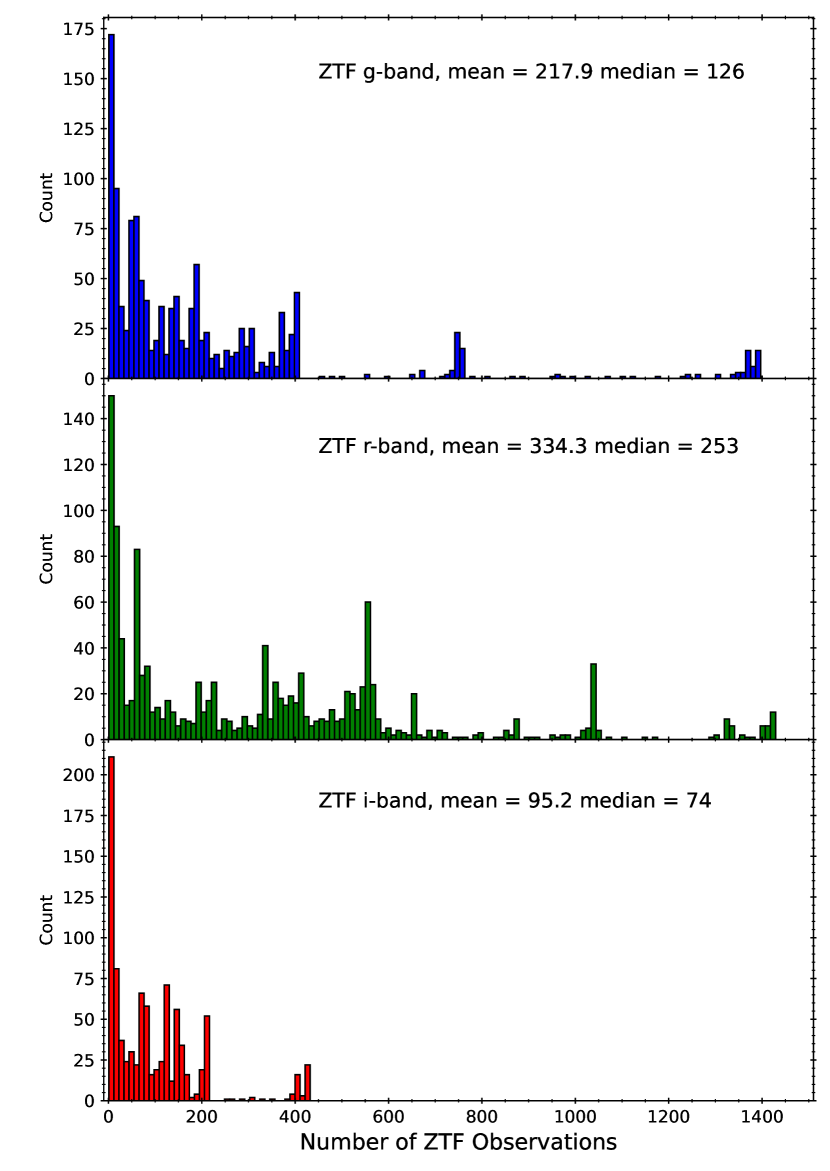
Figure 1: Histograms of the number of ZTF observation for our sample of RR Lyrae in the globular clusters. The mean and median numbers of observations were also given in the upper-right corner in each panels.

ZTF $gri$-band light curves were extracted for our sample of RR Lyrae from the PSF catalogs available from both of the ZTF Public Data Release 7 (including both public and Caltech data) and the partner surveys until 30 September 2021. Using a matching radius of $1\arcsec$, $gri$-band light curves of 1329 RR Lyrae in our initial list, whenever available, were extracted. Distributions of the number of data points per light curves $N$ (in the $gri$-band separately) are presented in Figure 1, where $N$ can be as large as $\sim 1390$ in the $gr$-band. The number of data points in the $i$-band light curves is much smaller due to combination of several reasons, such as late arrival of the $i$-band filter, the ZTF public surveys were conducted in the $gr$-band only, and the observing strategies for ZTF partnership surveys were focused on $gr$-band in the early time. Out of the 1329 RR Lyrae in our sample, 1328 of them have ZTF data in either $g$- or $r$-band (or both), but only 907 RR Lyrae have ZTF observations in the $i$-band.

2.4 Light Curve Fittings

Template light curve fitting approach was adopted to derive the mean magnitudes in $gri$-band for our sample of RR Lyrae. Since we do not have well-constrained amplitudes for RR Lyrae in our sample, we solved for the amplitude, phase shift, and mean magnitude as free parameters. Given that the minimum number of data points per phased light curve to fit with a template light curve is $3$ to account for the scaling (i.e. amplitude), the $x$-shift (i.e. the phase shift) and the $y$-shift (i.e. the mean magnitude) of the light curves, we further restricted the fitting to be performed only on the ZTF light curve in any bands that contains at least $3$ data points. The RRLyraeTemplateModelerMultiband module available in the astroML/gatspy package (hereafter gatspy; VanderPlas & Ivezić, 2015) was employed to fit the ZTF light curves using the $gri$-band template light curves derived in Sesar et al. (2010). During the light curves fitting, periods of the RR Lyrae were also revised from the initial values given in the Clement’s Catalog, as improvements in the fitted light curves can be seen on these RR Lyrae.

By default, gatspy will fit a given light curve with both RR0 and RR1 template light curves. Since the pulsation types of our sample of RR Lyrae are known from the Clement’s Catalog, we modified the gatspy code to only use either the RR0 or RR1 template light curves for a given RR Lyrae. To remove dubious outliers in the light curves, we adopted a two-iterations process: we first fit the ZTF light curves with the template light curves and data points that are more than $3s$ from the fitted light curves were removed ($s$ is the dispersion of the fitted light curve), and refit the template light curves on the remaining data points. The outputs of our light curve fitting procedures include the improved pulsation period $P$, the intensity-averaged mean magnitudes $\langle m\rangle$ and amplitudes $AMP_{m}$, where $m=\{g,\ r,\ i\}$ (whenever available), for each RR Lyrae based on the best-fit template light curves.

2.5 Errors Estimation on Mean Magnitudes

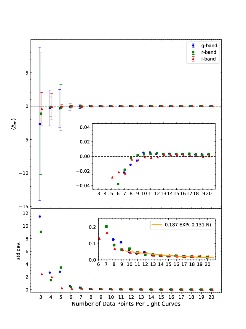
Figure 2: Results on errors estimation, based on simulated light curves (see text for details), for the mean magnitudes obtained with template light curve fittings. For a better visualization, the $g$- and $i$-band data points were offset slightly on the $x$-axis. Upper panel presents the averaged $\Delta_{m}$, obtained from 1000 simulated light curves, as a function of $N$, the number of data points per light curves. The error bars represent $1\sigma$ standard deviation on the averaged values. The horizontal dashed lines represent $\langle\Delta_{m}\rangle=0$. The inset figure in the upper panel is an enlarged version with error bars being omitted for clarity. In the lower panel, the corresponding standard deviations were plotted as a function of $N$. The orange curve in the inset figure is the best-fit exponential decay function to describe the trend of the standard deviations, at which the fittings of the exponential decay function were only done on data points with $N\geq 10$.

We ran Monte Carlo simulations to evaluate the errors on the mean magnitudes based on our procedures described above. Since template light curves fitting in gatspy is computationally intensive, we selected nine RR Lyrae that have more than 100 data points per light curves, as well as the dispersions on the final fitted light curves were smaller than $0.05$, in all three bands as our sample to run the Monte Carlo simulations. The fitted mean magnitudes of these nine RR Lyrae were considered as the “true values” in our simulations. To create a “simulated” light curve, we randomly selected one RR Lyrae out of the nine RR Lyrae, and for this selected RR Lyrae, we randomly picked $N$ data points without replacement, using a uniform random number generator, from the ZTF light curves. The simulated light curve was fitted with the two-steps template light curves fitting procedure as described previously to determine its mean magnitude which was compared with the “true value” to determine the difference $\Delta_{m}=FIT_{m}-TRUE_{m}$. We generated 1000 such simulated light curves, separately in the $gri$-band, to built up the distributions of $\Delta_{m}$, for $N$ spanning from $3$ to $20$. Averaged $\Delta_{m}$ and the associated standard deviations, were then calculated for each $N$ separately in the $gri$-band and presented in Figure 2.

It is clear from Figure 2 that the largest averaged $\Delta_{m}$ and standard deviation occurred when $N=3$ and hence the template light curves fitting should not be applied to light curves with only three data points. In the case of a small number of clustered data points, the templates fits can give very large amplitudes resulting in unrealistically large scatter in the mean magnitudes. Furthermore, the averaged $\Delta_{m}$ values exhibit a trend for $N<10$, and stabilized when $N\geq 10$ with values within $\pm 0.005$ mag. Hence, the template light curves fitting procedures should only be applied to light curves with $N\geq 10$. Large standard deviation can be seen when $N$ is less than 9, which decreases substantially for large $N$. An exponential decay function in the form of $f(N)=0.187\mathrm{e}^{-0.131N}$ can be used to fit the standard deviations when $N\geq 10$. Therefore, the calculated values of standard deviation based on $f(N)$ is $0.051$ mag at $N=10$, reduced to $0.014$ mag at $N=20$, and smaller than $0.001$ mag when $N>40$. Standard deviations calculated from $f(N)$ would be adopted as an error estimate for the mean magnitudes.

3 Further Filtering of RR Lyrae Sample

Table 2: List of globular clusters and the number of RR Lyrae in the sample.

G.C.	$\mathrm{[Fe/H]}$ (dex)	$n^{RR0}_{g}$	$n^{RR0}_{r}$	$n^{RR0}_{i}$	$n^{RR1}_{g}$	$n^{RR1}_{r}$	$n^{RR1}_{i}$	$n_{\mathrm{tot}}$	$D$ (kpc)	$\langle E\rangle$
NGC6426	$-2.36\pm 0.03$	7	7	0	5	5	0	12	$20.71\pm 0.35$	0.366
M30	$-2.33\pm 0.03$	3	4	0	2	2	0	6	$8.46\pm 0.09$	0.000
M15	$-2.27\pm 0.01$	53	50	47	53	48	39	109	$10.71\pm 0.10$	0.141
M92	$-2.27\pm 0.06$	11	10	10	6	6	6	17	$8.50\pm 0.07$	0.000
M68	$-2.25\pm 0.02$	14	14	0	16	16	0	30	$10.40\pm 0.10$	0.084
NGC5053	$-2.24\pm 0.16$	6	6	5	4	4	4	10	$17.54\pm 0.23$	0.001
NGC2419	$-2.12\pm 0.16$	26	27	18	30	30	15	57	$88.47\pm 2.40$	0.134
NGC5897	$-1.99\pm 0.03$	3	3	0	3	3	0	6	$12.55\pm 0.24$	0.089
NGC4147	$-1.95\pm 0.09$	5	5	5	10	10	10	15	$18.54\pm 0.21$	0.000
M22	$-1.92\pm 0.02$	10	10	0	13	14	0	24	$3.30\pm 0.04$	0.356
NGC6293	$-1.92\pm 0.10$	2	2	0	2	2	0	4	$9.19\pm 0.28$	0.410
M53	$-1.90\pm 0.05$	29	29	28	29	30	28	59	$18.50\pm 0.18$	0.004
Palomar13	$-1.85\pm 0.16$	4	4	4	0	0	0	4	$23.48\pm 0.40$	0.109
NGC5466	$-1.82\pm 0.08$	12	13	13	7	7	7	20	$16.12\pm 0.16$	0.005
M56	$-1.80\pm 0.15$	1	1	1	2	2	2	3	$10.43\pm 0.14$	0.191
NGC5634	$-1.77\pm 0.04$	8	9	7	6	6	6	15	$25.96\pm 0.62$	0.073
M80	$-1.72\pm 0.04$	6	5	0	6	6	0	12	$10.34\pm 0.12$	0.210
M19	$-1.70\pm 0.05$	1	1	0	0	0	0	1	$8.34\pm 0.16$	0.330
M9	$-1.70\pm 0.08$	7	7	0	8	8	0	15	$8.30\pm 0.14$	0.373
NGC7492	$-1.67\pm 0.12$	1	1	1	2	2	2	3	$24.39\pm 0.57$	0.029
Palomar3	$-1.60\pm 0.16$	6	6	3	0	0	0	6	$94.84\pm 3.23$	0.004
M79	$-1.57\pm 0.02$	5	5	0	3	3	0	8	$13.08\pm 0.18$	0.009
NGC7006	$-1.57\pm 0.05$	48	41	39	4	3	2	53	$39.32\pm 0.56$	0.136
M13	$-1.55\pm 0.05$	1	1	1	8	7	6	9	$7.42\pm 0.08$	0.000
M2	$-1.51\pm 0.02$	21	21	15	10	11	8	32	$11.69\pm 0.11$	0.016
M3	$-1.48\pm 0.05$	101	132	88	24	35	18	167	$10.18\pm 0.08$	0.035
NGC6934	$-1.48\pm 0.11$	61	62	55	8	8	7	72	$15.72\pm 0.17$	0.098
NGC6355	$-1.46\pm 0.06$	4	4	0	1	1	0	5	$8.65\pm 0.22$	0.865
Palomar5	$-1.38\pm 0.16$	0	0	0	5	5	0	5	$21.94\pm 0.51$	0.086
NGC6235	$-1.37\pm 0.08$	1	2	0	1	1	0	3	$11.94\pm 0.38$	0.379
M72	$-1.35\pm 0.08$	34	35	0	6	6	0	41	$16.66\pm 0.18$	0.041
NGC6229	$-1.35\pm 0.16$	40	36	33	15	15	15	55	$30.11\pm 0.47$	0.096
NGC288	$-1.33\pm 0.03$	1	1	1	1	1	0	2	$8.99\pm 0.09$	0.015
M14	$-1.28\pm 0.07$	4	5	0	6	7	0	12	$9.14\pm 0.25$	0.552
M28	$-1.18\pm 0.05$	10	10	9	7	7	6	17	$5.37\pm 0.10$	0.457
NGC6717	$-1.17\pm 0.09$	1	1	0	0	0	0	1	$7.52\pm 0.13$	0.258
M4	$-1.12\pm 0.02$	31	31	0	14	14	0	45	$1.85\pm 0.02$	0.385
M5	$-1.12\pm 0.01$	85	81	75	36	36	35	121	$7.48\pm 0.06$	0.094
NGC6401	$-1.08\pm 0.06$	22	23	15	11	9	7	34	$8.06\pm 0.24$	1.038
NGC6284	$-1.07\pm 0.05$	4	4	0	0	0	0	4	$14.21\pm 0.42$	0.318
NGC6642	$-1.03\pm 0.17$	7	7	0	3	3	0	10	$8.05\pm 0.20$	0.469
M75	$-1.01\pm 0.04$	15	13	0	5	6	0	21	$20.52\pm 0.45$	0.225
M107	$-1.00\pm 0.02$	15	15	0	6	6	0	21	$5.63\pm 0.08$	0.424
NGC6712	$-0.97\pm 0.05$	7	6	6	6	6	3	13	$7.38\pm 0.24$	0.414
NGC6638	$-0.89\pm 0.05$	3	5	0	9	10	0	15	$9.78\pm 0.34$	0.424
NGC6366	$-0.59\pm 0.04$	1	1	0	0	0	0	1	$3.44\pm 0.05$	0.730
NGC6544	$-1.37\pm 0.07$	1	1	1	0	0	0	1	$2.58\pm 0.06$	0.767
2MASS-GC02	$-1.05\pm 0.16$	0	0	0	0	1	1	1	$5.50\pm 0.44$	1.650
Terzan10	$-0.97\pm 0.16$	0	2	2	0	0	0	2	$10.21\pm 0.40$	2.029
Djorg2	$-0.91\pm 0.05$	1	1	0	2	2	0	3	$8.76\pm 0.18$	1.059
NGC6540	$-0.89\pm 0.73$	2	2	2	1	1	1	3	$5.91\pm 0.27$	0.619
IC1276	$-0.53\pm 0.05$	1	1	1	0	0	0	1	$4.55\pm 0.25$	1.156
NGC6316	$-0.46\pm 0.04$	1	1	0	1	1	0	2	$11.15\pm 0.39$	0.707
NGC6304	$-0.43\pm 0.05$	0	0	0	1	1	0	1	$6.15\pm 0.15$	0.658

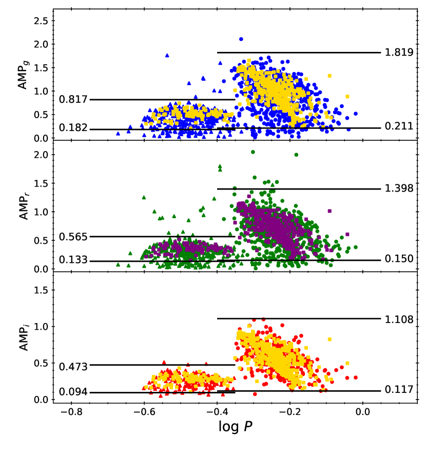
Figure 3: Comparison of the amplitudes for the RR Lyrae in our sample (represented in blue, green and red colors for the $gri$-band, respectively) and the RR Lyre located in the SDSS stripe 82 region (adopted from Sesar et al., 2010, shown as square symbols with either gold or purple colors). RR Lyrae in our sample with type RR0 (or RRab) and RR1 (or RRc) are marked with circles and triangles, respectively. The horizontal lines represent the adopted amplitude cuts in each filters, separated for RR0 and RR1, with values given next to these lines (see text for more details).

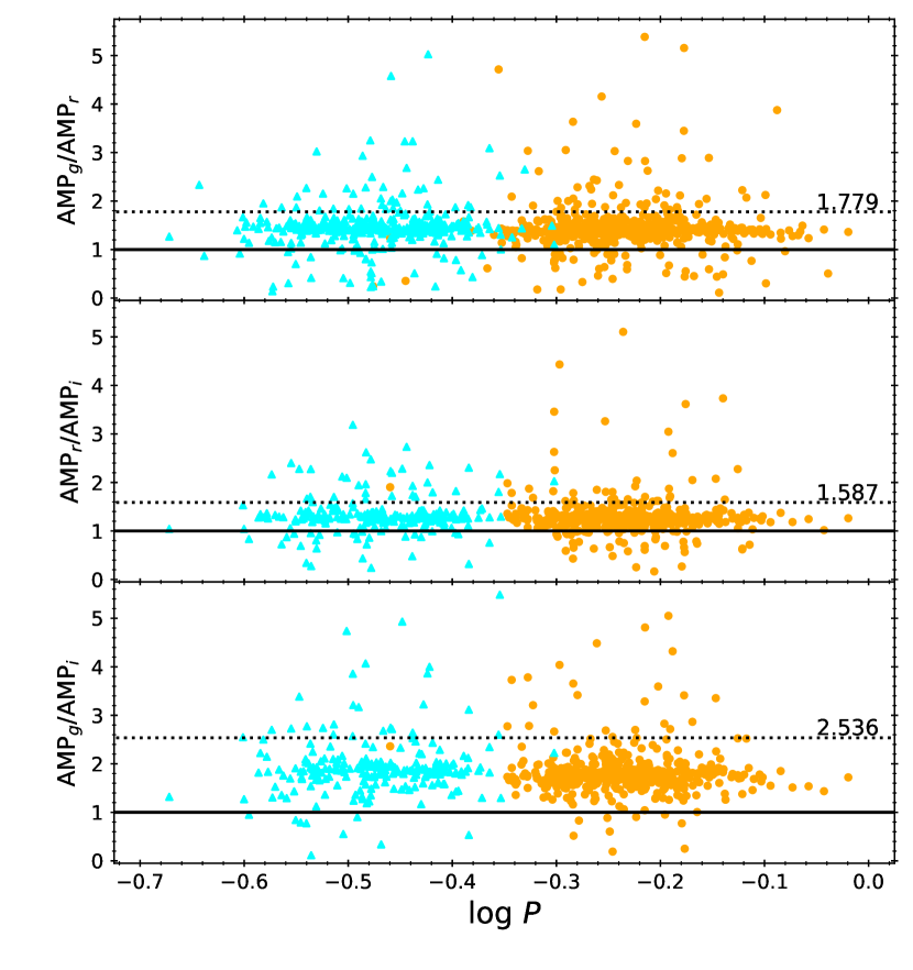
Figure 4: The $gri$-band amplitude ratios as a function of pulsation periods for the RR Lyrae in our sample, marked as filled orange circles and cyan triangles for the RR0 and RR1, respectively. The horizontal solid lines represent the amplitude ratios of unity. The dotted lines are the adopted upper limits for the amplitude ratio cuts (see text for more details).

Based on the results obtained in Section 2.5, we removed 120 RR Lyrae that have $N<10$ in all three filters after the second iteration in our template light curves fitting procedure, which leaves 1209 RR Lyrae in our sample. These remaining RR Lyrae are located in 54 globular clusters, as summarized in Table 2 along with their number, and the metallicity, extinction and the distance to each cluster. We further visually inspected a subset of the light curves for this sample of RR Lyrae and found that a fraction of the fitted light curves were problematic. For examples, some of these problematic light curves contain small number of data points that clustered at certain pulsational phases, or the light curves having mis-matched data points from very close-by neighboring sources (due to crowded nature of globular clusters). In many cases, these problematic light curves were found to be caused by blending. Due to highly crowded nature of globular clusters, blending is an unavoidable issue for RR Lyrae located near the center, or core, of the globular clusters. The inclusion of the fluxes from very close and yet unresolved constant stars will have two effects on the RR Lyrae light curves: making the RR Lyrae to appear brighter and the amplitudes of the RR Lyrae light curves will be greatly “damped” or reduced. A similar discussion on Cepheid’s light curve due to blending can be found in Riess et al. (2020). Therefore, those RR Lyrae affected by blending, as well as other problematic light curves, should be excluded.

3.1 Filtering Based on Amplitudes

We first examined amplitudes of the RR Lyrae remained in our sample. Since the light curve amplitudes for pulsating stars cannot be arbitrary large, fitted light curves with large amplitudes indicated there were some problems related to the sampling of the light curves. Similarly, if the light curve amplitudes are too small this would hint the presence of blending. The $gri$-band amplitudes for our sample of RR Lyrae are shown in Figure 3, overlaid with a sample of 483 RR Lyrae located in the Sloan Digital Sky Survey (SDSS) Stripe 82 region (Sesar et al., 2010). The SDSS Stripe 82 RR Lyrae samples are located in the Galactic halo, hence they are expected to be unaffected by blending. Clearly, amplitudes for some of our sample of RR Lyrae were either larger or smaller than those laid out by the SDSS Stripe 82 RR Lyrae, which can be used to define the amplitude cuts. To account for the possibility that the RR Lyrae in the globular clusters may have larger amplitudes, the maximum amplitudes found in the SDSS Stripe 82 RR Lyrae were then increased by $10\%$ and adopted as the maximum amplitude cuts. Similarly, the minimum amplitude cuts were based on the minimum amplitudes found in the SDSS Stripe 82 RR Lyrae but decreased by $10\%$. These adopted amplitude cuts were shown as horizontal lines in Figure 3.

Amplitude ratios between different filters can also be used to filter out the problematic light curves. Figure 4 presents the derived amplitude ratios for our sample of RR Lyrae, at which majority of the RR Lyrae fall in a tight sequence. Since the amplitudes for RR Lyrae are larger at shorter wavelength filters (for examples, see Braga et al., 2016; Bhardwaj et al., 2020), amplitude ratios as defined in Figure 4 should have values larger than unity (indicated with solid lines in Figure 4). However, there are a number of outliers with unusually large amplitude ratios. Therefore, we first exclude those RR Lyrae in our sample with amplitude ratios smaller than unity, the remaining RR Lyrae were used to estimate the averaged amplitude ratios via an iterative $3\sigma$-clipping algorithm, which were found to be:

$$\langle\frac{AMP_{g}}{AMP_{r}}\rangle=1.419,\ \langle\frac{AMP_{r}}{AMP_{i}}\rangle=1.266,\ \langle\frac{AMP_{g}}{AMP_{i}}\rangle=1.782,$$

with corresponding standard deviations of $0.120$, $0.107$, and $0.251$, respectively. The lower limit of the amplitude ratio cut is 1. For the upper limit, we adopted a value that is three times of the standard deviation larger than the averaged amplitude ratio, indicated by the dotted lines in Figure 4. While deriving these averaged values (and their standard deviations), we did not separate out the RR0 and RR1 because the derived averaged values do not show a significant deviation between them (for example, the averaged $gr$-band amplitude ratios are $1.405$ and $1.452$ for RR0 and RR1, respectively).

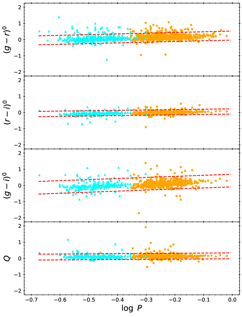
Figure 5: Extinction corrected period-color (PC, top three panels) relations and the extinction-free $Q$-indices as a function of pulsation periods (i.e. the PQ relation, bottom panel) for the RR Lyrae in our sample, separated for RR0 (filled orange circles) and RR1 (filled cyan triangles). The red dashed lines indicate the selection boundaries based on the provisional fitted PC/PQ relations to the RR0 and RR1 combined samples (see text for more details).

Combining the amplitude cuts as given in Figure 3 and the amplitude ratio cuts as shown in Figure 4 (the dotted and the solid lines), there are 331 RR Lyrae in our sample (out of 1209) which did not satisfy the selection criteria based on either the amplitudes or amplitude ratios, or both. These RR Lyrae were flagged as “A” in our sample.

3.2 Filtering Based on Colors

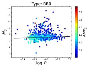
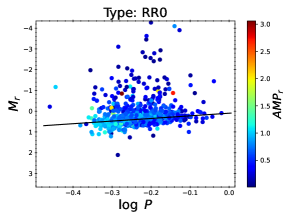
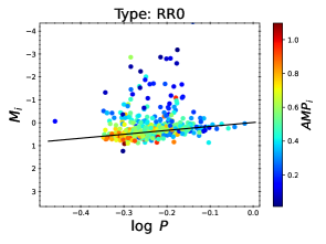
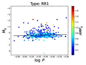
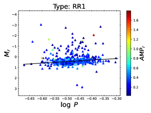
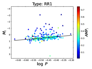
Figure 6: The composite $gri$-band period-luminosity (PL) relations based on the 1209 RR Lyrae in different globular clusters, separated for RR0 (upper panels) and RR1 (lower panels). The solid lines are the provisional fitted PL relations (see text for details). For clarity, error bars are omitted. Colors on the data points represent the amplitudes derived from the best-fit template light curves.

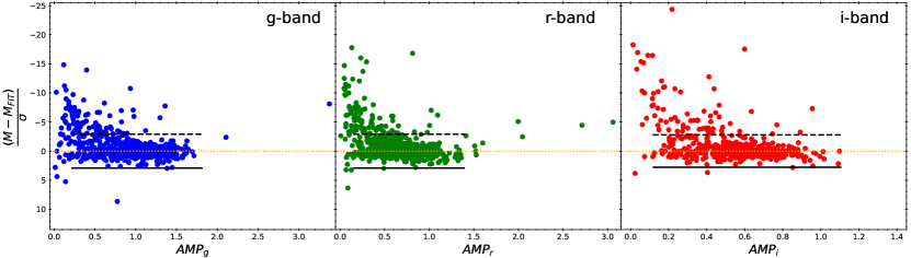
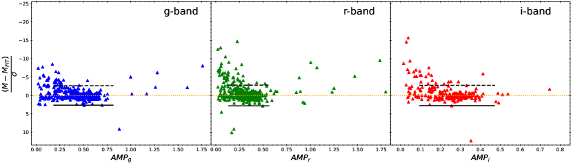
Figure 7: Residuals of the fitted PL relations given in Figure 6, in the unit of the PL dispersion $\sigma$, as a function of the light curve amplitudes. The dotted (orange) horizontal line represents the zero residuals to guide the eyes. The solid horizontal lines are the boundaries on the positive residuals determined using the boundfit code (Cardiel, 2009, see text for more details). The dashed horizontal lines are the boundaries on the negative residuals mirrored from the solid horizontal lines. Size of these horizontal lines were based on the adopted amplitude cuts (see Figure 3). Upper and lower panels are for RR0 (in filled circles) and RR1 (in filled triangles), respectively.

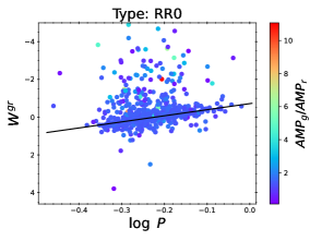
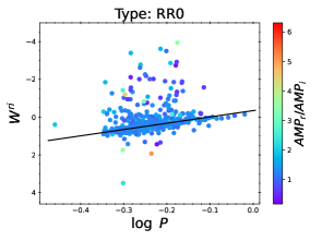
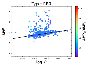
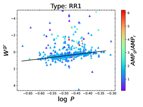
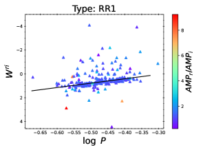
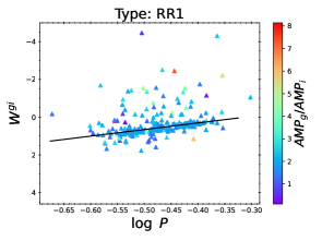
Figure 8: The composite period-Wesenheit (PW) relations based on the 1209 RR Lyrae in different globular clusters, separated for RR0 (upper panels) and RR1 (lower panels). The solid lines are the provisional fitted PW relations (see text for details). For clarity, error bars are omitted. Colors on the data points represent the amplitude ratios derived from the best-fit template light curves.

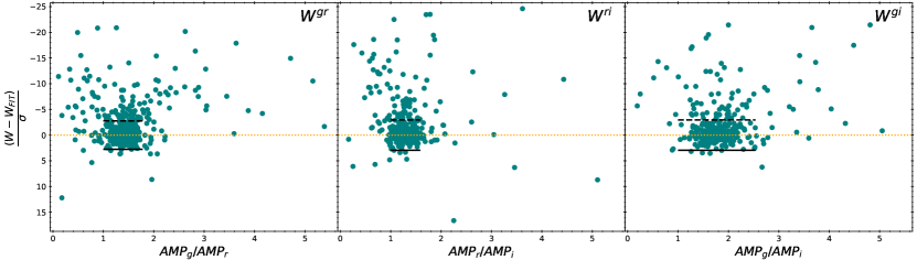
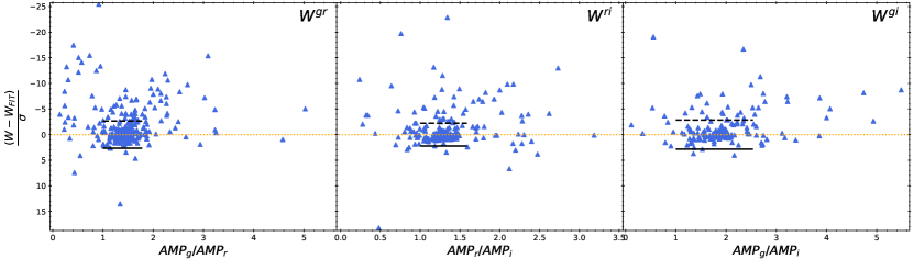
Figure 9: Residuals of the fitted PW relations given in Figure 8, in the unit of the PW dispersion $\sigma$, as a function of the amplitude ratios. The dotted (orange) horizontal line represents the zero residuals to guide the eyes. The solid horizontal lines are the boundaries on the positive residuals determined using the boundfit code (Cardiel, 2009, see text for more details). The dashed horizontal lines are the boundaries on the negative residuals mirrored from the solid horizontal lines. Size of these horizontal lines were based on the adopted amplitude ratio cuts (see Figure 4). Upper and lower panels are for RR0 (in filled circles) and RR1 (in filled triangles), respectively.

As pulsating stars, RR Lyrae are expected to obey a period-color (PC) relation. Therefore, outliers presented on the plot of the PC relation indicate their corresponding light curves could be problematic. Top panels of Figure 5 present the extinction-corrected PC relations for the RR Lyrae in our sample, at which the mean magnitudes in each filters were corrected using $R_{\{g,r,i\}}E$. The values of extinction coefficient are $R_{\{g,r,i\}}=\{3.518,\ 2.617,\ 1.971\}$ (Green et al., 2019) because ZTF photometry is calibrated to the Pan-STARRS1 system (Masci et al., 2019), and the reddening $E$ toward each of the RR Lyrae was obtained using the Bayerstar2019 3D reddening map (Green et al., 2019, see Section 2.2).

In Figure 5, majority of the RR Lyrae show a tight and continuous PC relation for the RR0 and RR1 combined sample, but outliers were also presented in these PC relations. Most of these outliers were either having the amplitude or the amplitude ratios beyond the respected cuts as defined in previous subsection. To remove these outliers, an iterative linear regression with $3\sigma$ outliers rejection algorithm was applied to fit both RR0 and RR1. The $3\sigma$ boundaries from the provisional fitted PC relations, displayed as dashed lines in Figure 5, were adopted as the period-dependent color cuts. Note that fitting of the PC relations, separately for RR0 and RR1, on our final sample will be done in Section 5.

To circumvent the possibility that the outliers shown in Figure 5 were (partly) due to the extinction, we plotted the extinction-free $Q$-indices as a function of pulsation periods in the bottom panel of Figure 5 for RR Lyrae that have mean magnitudes in all $gri$ bands. Given the adopted values of $R_{\{g,r,i\}}$, the extinction-free $Q$-index is defined as:

$$Q = (g-r)-1.395(r-i).$$

Similar to the PC relations, we derived a provisional PQ relation, and the $3\sigma$ boundaries were adopted as the period-dependent $Q$-index cuts, shown as the dashed lines in the bottom panel of Figure 5.

In total, there are 147 RR Lyrae located outside the $3\sigma$ boundaries of either the three PC relations or the PQ relation. These RR Lyrae were flagged as “C” in our sample.

3.3 Filtering Based on PL/PW Residuals

Figure 6 presents the extinction-corrected $gri$-band PL relations for our sample of RR Lyrae. The mean magnitudes $\langle m\rangle$ for these RR Lyrae were converted to absolute magnitudes using $M_{\{g,r,i\}}=\langle m_{\{g,r,i\}}\rangle-R_{\{g,r,i\}}E-5\log D+5$, where the extinction term ($R_{\{g,r,i\}}E$) was described in Section 3.2, and the distance $D$ was adopted from Baumgardt & Vasiliev (2021, see Section 2.2). Errors from $\langle m\rangle$, $E$, and $D$ were propagated to the total errors on $M$.

As mentioned, blending would cause a RR Lyrae to appear brighter, at the same time the amplitude of such RR Lyrae would be reduced. As can be seen from Figure 6, there are a number of RR Lyrae that seem to be brighter than the rest of the RR Lyrae at a given period. These RR Lyrae also tend to have smaller amplitudes obtained from the best-fit template light curves, suggesting these RR Lyrae were most likely affected by blending and should be excluded. A provisional period-luminosity (PL) relation in the form of $M_{FIT}=a\log P+b$, separately for RR0 and RR1, was fitted to our sample of RR Lyrae, where the fitting was performed using an iterative $3\sigma$-rejection procedure to remove the outliers until the fitted parameters $a$ and $b$ converged. The fitted provisional PL relations were marked as solid lines in Figure 6.

To better visualize the effects of blending, residuals of the fitted PL relations, in the unit of PL dispersion $\sigma$, i.e. $(M-M_{FIT})/\sigma$, were plotted against the amplitudes determined from the best-fit template light curves in Figure 7, showing that more negative residuals (i.e. brighter than expected) tend to have a smaller amplitude. After excluding RR Lyrae with $(M-M_{FIT})/\sigma>3$ (based on the adopted iterative $3\sigma$-rejection linear regression fitting) and those with amplitudes outside the amplitude cuts defined in Figure 3, we determined the one-site boundaries on the positive residuals by using the boundfit code (Cardiel, 2009). These boundaries are indicated by solid horizontal lines in Figure 7. Since the residuals of the PL relation should be symmetric, these boundaries were then mirrored to the negative residuals and presented as dashed horizontal lines in Figure 7. RR Lyrae with negative residuals that were more negative than the dashed horizontal lines are brighter than expected, implying these RR Lyrae could be affected by blending (which also tend to have smaller amplitudes).

In addition to the PL relations, we have also examined the PW relation for our sample of RR Lyrae. The extinction-free Wesenheit indexes were defined as (Ngeow et al., 2021):

$$W^{gr} = r-2.905(g-r),$$

$$W^{ri} = r-4.051(r-i),$$

$$W^{gi} = g-2.274(g-i).$$

The corresponding PW relations are presented in Figure 8, together with the provisional PW relations (fitted with the same iterative $3\sigma$-rejection algorithm as in the case of provisional PL relations) shown in the solid lines. Data points in Figure 8 were also color-coded with amplitude ratios. There are two features revealed from Figure 8. First of all, majority of the outliers are brighter than those RR Lyrae located along the ridge lines at a given period, again indicating the presence of blending. Secondly, RR Lyrae along the ridge lines have similar, or consistent amplitude ratios, while the outliers either have a large or a small (i.e., smaller than unity) amplitude ratio.

Residuals of the provisional PW relations, in unit of PW dispersion $\sigma$, as a function of amplitude ratios were presented in Figure 9. It is clear that RR Lyrae with small PW residuals (e.g., $<|3\sigma|$) also tend to concentrate on a small range of amplitude ratio, iterating the similar concentration in Figure 4. Similar to the PL residuals, we used boundfit to determine the one-site boundaries on the positive residuals after excluding the outlying residuals with $(W-W_{FIT})/\sigma>3$ and outside the amplitude ratio cuts given in Figure 4. The determined one-site boundaries were then mirrored to the negative residuals. These boundaries were shown as solid and dashed horizontal lines in Figure 9.

Based on the residuals from the PL or PW relations, there were 306 RR Lyrae with residuals beyond the boundaries determined in either Figure 7 or 9 (both solid and dashed lines). These RR Lyrae were flagged as “R” in our sample.

3.4 The Final Sample of RR Lyrae

Figure 10: Venn diagram for the excluded RR Lyrae in our sample (see text for details on flag “A”, “C”, and “R”).

Figure 11: Examples of the light curves for RR Lyrae with 3 (top panels), 2 (middle panels), and 1 (bottom panels) of the “ACR” flags. The black crosses are rejected data points during the first pass of the two-iterations template light curve fitting procedure, and the black curves are the best-fit template light curves after the second pass of the procedure (see Section 2.4 for more details).

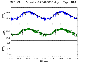
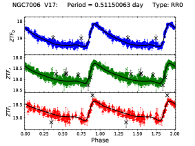
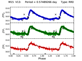
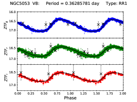
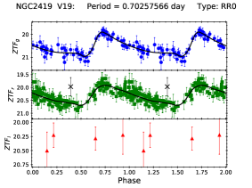
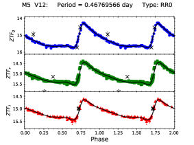
Figure 12: Examples of the randomly selected light curves for RR Lyrae without any flags. The black crosses are rejected data points during the first pass of the two-iterations template light curve fitting procedure, and the black curves are the best-fit template light curves after the second pass of the procedure (see Section 2.4 for more details).

The refined periods and reddenings, as well as the mean magnitudes, amplitudes and number of data points left in the $gri$-band light curves for the 1209 RR Lyrae in our sample are presented in Table 3. In the last column of Table 3 we also included the flags for each RR Lyrae based on the analysis given in previous subsections. Out of the 1209 RR Lyrae in our sample, 108 have all three “ACR” flags. The number of RR Lyrae with two flags is 114 (8, 23 and 83 with “AC”, “CR” and “AR”, respectively), while the number of RR Lyrae with only one flag is 232 (132, 8 and 92 with “A”, “C” and “R”, respectively). A Venn diagram showing the distribution of these flagged RR Lyrae is presented in Figure 10. Example light curves for these flagged RR Lyrae are shown in Figure 11 for the cases with 3, 2, and 1 flag, showing that the light curves for RR Lyrae with any of the “ACR” flags, or a combination of them, were problematic due to a variety of reasons and should be excluded.

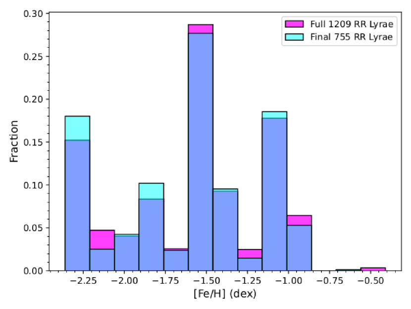
Figure 13: Histograms of $[\mathrm{Fe/H}]$ distribution for the full sample of 1209 RR Lyrae and the remaining sample of 755 RR Lyrae in our sample. The $[\mathrm{Fe/H}]$ values for the RR Lyrae are based on their host globular clusters (see Table 2).

The remaining 755 RR Lyrae in our sample do not carry any of the “ACR” flags. Examples of their light curves are presented in Figure 12, demonstrating the good quality of the ZTF light curves for them. These sample of RR Lyrae will be used to derive the PLZ and PWZ relation in the next section, and they are located in 46 (out of 54) globular clusters. The excluded globular clusters are (as listed in the bottom of Table 2): 2MASS-GC02, Djorg2, IC1276, NGC6304, NGC6316, NGC6540, NGC6544 and Terzan10, as all of their RR Lyrae have one or more flags. These also removed the three globular clusters with highest metallicities (IC1276, NGC6316, and NGC6304), hence the range of metallicity covered by the 755 RR Lyrae is from $-2.36$ dex to $-0.54$ dex, with a median of $-1.48$ dex. Figure 13 compares the metallicity distribution between the “full” sample of 1209 RR Lyrae and the remaining sample of 755 RR Lyrae, no substantial difference can be seen between their distributions. This ensures there is no bias introduced when fitting the PLZ and PWZ relations to the remaining 755 RR Lyrae sample.

Table 3: Periods, mean magnitudes, amplitudes and reddenings for our sample of RR Lyrae.

Var. Name	Type	Period (days)	$\langle m_{g}\rangle$	$AMP_{g}$	$N_{g}$	$\langle m_{r}\rangle$	$AMP_{r}$	$N_{r}$	$\langle m_{i}\rangle$	$AMP_{i}$	$N_{i}$	$E$	Flag
Palomar3_V2	RR0	0.59867205	20.512	0.742	92	20.301	0.597	121	20.215	0.293	10	$0.004\pm 0.002$	A__
Palomar3_V3	RR0	0.56690511	20.469	0.872	107	20.269	0.661	120	20.150	0.431	12	$0.004\pm 0.002$	__R
Palomar3_V5	RR0	0.58168014	20.518	0.846	97	20.327	0.585	128	20.209	0.379	10	$0.004\pm 0.002$	___
Palomar3_V6	RR0	0.59336755	20.493	0.916	83	20.311	0.583	60	-99.999	-9.999	7	$0.004\pm 0.002$	___
$\cdots$	$\cdots$	$\cdots$	$\cdots$	$\cdots$	$\cdots$	$\cdots$	$\cdots$	$\cdots$	$\cdots$	$\cdots$	$\cdots$	$\cdots$	$\cdots$

Note. — Table 3 is published in its entirety in the machine-readable format. A portion is shown here for guidance regarding its form and content. $AMP_{\{g,r,i\}}$ is the amplitude based on the best-fit template light curve. Values of $-99.990$ and $-9.990$ denote no data or rejected light curves. $N_{\{g,r,i\}}$ is the number of data points in a given filter after the two-steps template fitting processes as described in Section 2.3. $E$ is the reddening value returned from the Bayerstar2019 3D reddening map (Green et al., 2019) using the globular cluster distance listed in Table 2.

4 The PLZ and PWZ Relations

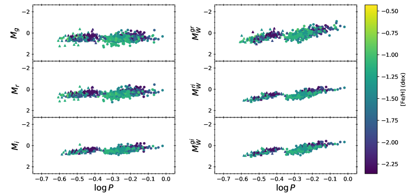
Figure 14: The PL relations (left panels, after corrected for extinction) and PW relations for all of the RR Lyrae listed in Table 3, by adopting the distance of the globular clusters as listed in Table 2. The color-bar represents the metallicity for the host globular clusters. Circular and triangle symbols are for the RR Lyrae with pulsation types of RR0 and RR1, respectively. Error bars are omitted for clarity.

Table 4: Fitted coefficients for various relations.

	$a$	$b$	$c$	$\sigma$	$N_{\mathrm{ini}}/N_{\mathrm{fit}}$
RR0 only
$M_{g}$	$0.649\pm 0.073$	$-0.302\pm 0.193$	$0.159\pm 0.024$	0.227	493/490
$M_{r}$	$0.337\pm 0.059$	$-1.090\pm 0.154$	$0.139\pm 0.020$	0.187	516/508
$M_{i}$	$0.243\pm 0.055$	$-1.432\pm 0.144$	$0.144\pm 0.018$	0.148	326/321
$W^{gr}$	$-0.644\pm 0.058$	$-3.324\pm 0.155$	$0.052\pm 0.020$	0.205	483/478
$W^{ri}$	$0.093\pm 0.051$	$-2.600\pm 0.133$	$0.193\pm 0.017$	0.145	326/325
$W^{gi}$	$-0.198\pm 0.054$	$-2.908\pm 0.142$	$0.142\pm 0.018$	0.146	325/323
$(g-r)$	$0.333\pm 0.023$	$0.764\pm 0.060$	$0.035\pm 0.007$	0.076	483/483
$(r-i)$	$0.040\pm 0.014$	$0.361\pm 0.038$	$-0.017\pm 0.004$	0.035	326/323
$(g-i)$	$0.323\pm 0.033$	$1.110\pm 0.088$	$-0.001\pm 0.010$	0.093	325/325
$Q$	$0.222\pm 0.016$	$0.220\pm 0.044$	$0.042\pm 0.005$	0.046	325/320
RR1 only
$M_{g}$	$0.411\pm 0.166$	$-0.342\pm 0.289$	$0.092\pm 0.028$	0.189	218/212
$M_{r}$	$-0.082\pm 0.138$	$-1.393\pm 0.238$	$0.091\pm 0.024$	0.164	227/224
$M_{i}$	$-0.205\pm 0.139$	$-1.706\pm 0.246$	$0.077\pm 0.023$	0.128	123/122
$W^{gr}$	$-1.327\pm 0.143$	$-3.680\pm 0.248$	$0.013\pm 0.024$	0.172	216/210
$W^{ri}$	$-0.884\pm 0.141$	$-3.503\pm 0.249$	$0.067\pm 0.023$	0.132	123/123
$W^{gi}$	$-1.086\pm 0.126$	$-3.696\pm 0.223$	$0.055\pm 0.020$	0.111	123/120
$(g-r)$	$0.398\pm 0.059$	$0.781\pm 0.103$	$0.017\pm 0.009$	0.069	216/215
$(r-i)$	$0.194\pm 0.039$	$0.569\pm 0.070$	$-0.005\pm 0.006$	0.030	123/121
$(g-i)$	$0.670\pm 0.101$	$1.545\pm 0.179$	$0.014\pm 0.016$	0.080	123/122
$Q$	$0.192\pm 0.029$	$0.162\pm 0.052$	$0.024\pm 0.004$	0.039	123/121
RR0 + RR1
$M_{g}$	$0.801\pm 0.048$	$-0.032\pm 0.110$	$0.190\pm 0.019$	0.216	711/704
$M_{r}$	$0.432\pm 0.039$	$-0.874\pm 0.089$	$0.154\pm 0.016$	0.180	743/731
$M_{i}$	$0.249\pm 0.041$	$-1.362\pm 0.093$	$0.115\pm 0.016$	0.138	449/444
$W^{gr}$	$-0.727\pm 0.041$	$-3.286\pm 0.093$	$0.010\pm 0.016$	0.191	699/687
$W^{ri}$	$0.010\pm 0.037$	$-2.756\pm 0.086$	$0.149\pm 0.015$	0.130	448/444
$W^{gi}$	$-0.288\pm 0.039$	$-3.066\pm 0.090$	$0.101\pm 0.015$	0.137	449/444
$(g-r)$	$0.333\pm 0.014$	$0.803\pm 0.034$	$0.030\pm 0.005$	0.073	699/697
$(r-i)$	$0.063\pm 0.009$	$0.428\pm 0.023$	$-0.012\pm 0.003$	0.033	449/444
$(g-i)$	$0.370\pm 0.022$	$1.263\pm 0.055$	$0.007\pm 0.007$	0.089	448/447
$Q$	$0.218\pm 0.009$	$0.222\pm 0.023$	$0.038\pm 0.003$	0.043	448/440

Note. — The fitting parameters $a$, $b$, and $c$ are defined in equation (1), and $\sigma$ is the dispersion of the fitted relation. $N_{\mathrm{ini}}$ and $N_{\mathrm{fit}}$ are the number of RR Lyrae before and after applying the $3\sigma$-rejection algorithm (the number of rejected RR Lyrae varies from 0 to 12). Note that $M_{gri}$ and various colors have been corrected for extinction.

The extinction-corrected $gri$-band PL and the PW relations for the final sample of 755 RR Lyrae were presented in the left and right panels of Figure 14, respectively, where the coded-colors represent the metallicity of the host globular clusters. These RR Lyrae were fitted with PLZ and PWZ relations in the following form:

$$y = a+b\log P+c[Fe/H],$$ (1)

where $y$ is either $M_{gri}$ or $W$, and all RR Lyrae in a given clusters are assumed to have the same distance as given in Table 2. We solved equation (1) using a $\chi^{2}$ minimization within a matrix formalism of dependent and independent parameters including their associated uncertainties in the covariance matrix (similar to equation (5) in Bhardwaj et al., 2016). As in Bhardwaj et al. (2021), we also applied an iterative $3\sigma$-rejection algorithm to remove the single largest outlier in each iteration until convergence. Figure 14 shows that there are still a few outliers presented in the PL and PW relations that were not flagged based on the selection criteria presented in Section 3. Their light curves look normal implying other physical reasons (such as location on the near-site of the host globular clusters, incorrect estimation of extinction, etc) causing them to become outliers on the PL and/or PW relations. Nevertheless, they should be excluded to obtain a more robust relation. The fitted coefficients and the corresponding dispersion are summarized in Table 4 for RR0 and RR1 separately, as well as the RR0 and RR1 combined sample. When combining RR0 and RR1 samples, periods for RR1 were fundametalized using $\log P_{0}=\log P_{1}+0.127$ (for examples, see Iben, 1974; Coppola et al., 2015), where $P_{1}$ and $P_{0}$ represent the first-overtone period and the corresponding fundametalized period.

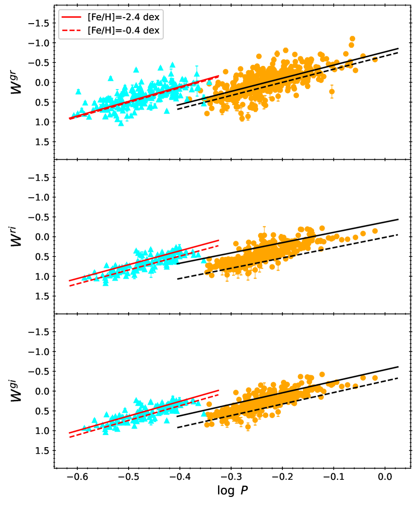
Figure 15: The metallicity-dependent period-Wesenheit (PWZ) relations for our sample of RR Lyrae. The solid and dashed lines (in both red and black colors) represent the PWZ relations evaluated at $[\mathrm{Fe/H}]=-2.4$ dex and $[\mathrm{Fe/H}]=-0.4$ dex, respectively. The orange circles and cyan triangles are for the RR0 and RR1, respectively. The PWZ relations for the combined sample of RR0 and RR1 (after fundametalized the periods) are similar, hence they are not included in this Figure.

In Figure 15 we present the fitted PWZ relations evaluated at $[\mathrm{Fe/H}]=-2.4$ dex and $-0.4$ dex. These two values of metallicities were chosen to bracket the metallicity listed in Table 2. As can be seen from left panel of Figure 15 and Table 4, the $W^{gr}$ PWZ relations show a very weak, or even vanishing, dependence on the metallicity for either RR0 or RR1, or the combined sample. Interestingly, similar metallicity-independent PW(Z) relations were found in Marconi et al. (2015) for Wesenheit indexes defined in the Johnson $BVR$ filters based on a series of theoretical models. We noted that the $gr$-band transmission curves covering a similar wavelength range as the Johnson $BVR$-band transmission curves. As discussed in Marconi et al. (2015), such a nearly metallicity-independent PW(Z) relation can be used as a robust distance indicator, however, the downside is our derived $W^{gr}$ PWZ relations exhibit a larger dispersion than other two Wesenheit indexes. Based on Table 4, we also notice that the fitted PLZ and PWZ relations involving $i$-band have the smallest dispersion.

In the following subsections, we compared our derived PLZ relations to published PL(Z) relations in $gri$-band, including three empirical and two theoretical PL(Z) relations. For an ease of comparisons, we summarized slopes of these PL(Z) relations in Table 5.

Table 5: Comparison of the slopes of PL(Z) relations from various studies.

Ref.	$g$-band	$r$-band	$i$-band	G.C.
For RR0
TW	$-0.302\pm 0.193$	$-1.090\pm 0.154$	$-1.432\pm 0.144$	46 G.C.
S17	$-1.7\pm 0.3$	$-1.6\pm 0.1$	$-1.77\pm 0.08$	5 G.C
V17	$-0.57\pm 0.17$	$-1.28\pm 0.11$	$-1.59\pm 0.09$	M5
B21	$-0.111\pm 0.160$	$\cdots$	$-1.292\pm 0.184$	M15
C08	$\cdots$	$\cdots$	$1.035$	$\cdots$
M06	$-0.311$	$\cdots$	$\cdots$	$\cdots$
For RR1
TW	$-0.342\pm 0.289$	$-1.393\pm 0.238$	$-1.706\pm 0.246$	46 G.C.
V17	$-0.72\pm 0.32$	$-1.35\pm 0.21$	$-1.61\pm 0.16$	M5
B21	$-0.019\pm 0.138$	$\cdots$	$-1.329\pm 0.112$	M15
M06	$-0.322$	$\cdots$	$\cdots$	$\cdots$
For RR0+RR1
TW	$-0.032\pm 0.110$	$-0.874\pm 0.089$	$-1.362\pm 0.093$	46 G.C.
B21	$+0.185\pm 0.066$	$\cdots$	$-1.222\pm 0.060$	M15

Note. — Slopes without errors are for the (semi-)theoretical PL(Z) relations. In case of RR0+RR1, periods for RR1 have been fundametalized. The references (Ref.) are: TW = this work (Table 4); S17 = Sesar et al. (2017); V17 = Vivas et al. (2017); B21 = Bhardwaj et al. (2021); C08 = Cáceres & Catelan (2008); and M06 = Marconi et al. (2006).

4.1 Comparisons to Published Results: Empirical Relations

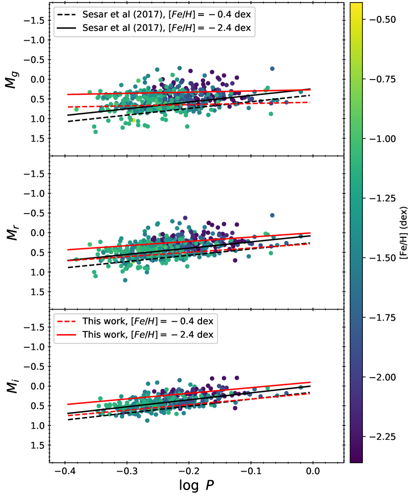
Figure 16: Comparison of the PLZ relations for RR0 from Sesar et al. (2017, in black colors) and this work (i.e. Table 4, in red colors), evaluated at two metallicities: $[\mathrm{Fe/H}]=-2.4$ dex and $-0.4$ dex as solid and dashed lines, respectively.

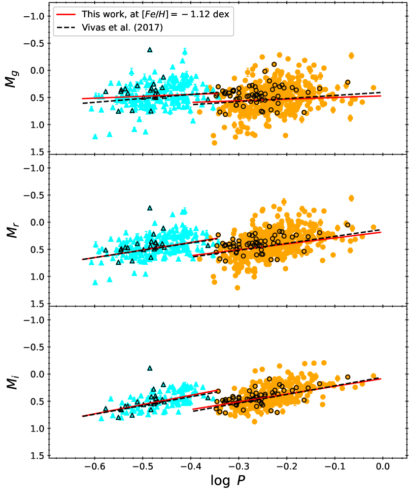
Figure 17: Comparison of the PL relations from Vivas et al. (2017, as black dashed lines) and this work (i.e. Table 4, as red solid lines), evaluated at $[\mathrm{Fe/H}]=-1.12$ dex for M5 (see Table 2). The orange circles and cyan triangles are for the RR0 and RR1 in our sample, respectively. Data points with black circles or triangles represent the RR Lyrae in M5.

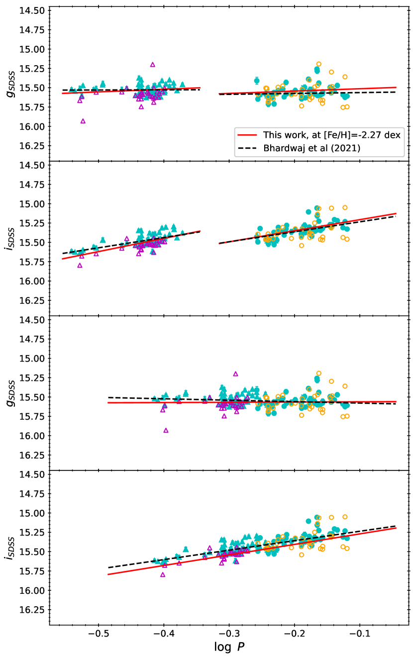
Figure 18: Comparison of the PL relations from Bhardwaj et al. (2021, as black dashed lines) and this work (i.e. Table 4, as red solid lines), evaluated at $[\mathrm{Fe/H}]=-2.27$ dex for M15 (see Table 2). The orange open circles and magenta open triangles are for the RR0 and RR1 in our sample, respectively, with mean magnitudes transformed to the SDSS system. Data points with filled light green circles or triangles represent the RR Lyrae taken from Bhardwaj et al. (2021). Consistent extinction of $A_{g}=0.379$ and $A_{i}=0.209$ (Bhardwaj et al., 2021) in the SDSS system were applied to all data points. Our PL relations were shifted vertically using the distance of M15 as listed in Table 2. The bottom two panels are for the combined sample of RR0 and RR1 after fundametalized the pulsation periods of RR1.

Sesar et al. (2017) derived PLZ relations in the $gri(z)$-band using a sample of 55 RR0 located in 5 globular clusters. We compared the $gri$-band PLZ relations derived in their work with ours in Figure 16, and found that these two sets of PLZ relations disagree with each other. For example, the metallicity terms for our PLZ relations are approximately twice the values reported in Sesar et al. (2017). Slopes of these PLZ relations even show a larger disagreement, especially for the $g$-band PLZ relations. Our $i$-band PLZ relation has a slope closer to the one derived in Sesar et al. (2017, $-1.432$ vs. $-1.77$), however these two slopes are different by $\sim 2\sigma$. Despite in common Pan-STARRS1 photometric system, the derivations of the PLZ relations between Sesar et al. (2017) and our work are significantly different, including data sources used, the adopted distances to the globular clusters, and the methodology of fitting the PLZ relations. Using a Bayesian inference approach, Sesar et al. (2017) adopted a tight Gaussian prior when fitting the slopes of the $ri$-band PLZ relations, but not in the $g$-band. This might explain why the slope of the $g$-band PLZ relation is much steeper in Sesar et al. (2017) than our derived value as presented in Table 4.

A similar comparison was also done on the PL relations derived in Vivas et al. (2017), using RR Lyrae in M5 observed with DECam. As evident in Figure 17, these two sets of PL relations are in remarkably good agreement for both RR0 and RR1 PL relations. Vivas et al. (2017) calibrated their photometry to the native DECam system, which has been extensively employed by the Dark Energy Survey (DES, Dark Energy Survey Collaboration et al., 2016), therefore the PL relations presented in Vivas et al. (2017) strictly speaking are in the DES photometric system. To transform the PL relations given in Vivas et al. (2017) from DES system to Pan-STARRS1 system, we added a correction term $\delta_{m}$ to their PL relations, separately in $gri$-band for RR0 and RR1. These $\delta_{m}$ were determined using the averaged colors of RR0 and RR1 based on the $\sim 60$ RR Lyrae listed in Vivas et al. (2017), together with the transformation provided in Abbott et al. (2021), and found to be small (range from $-0.024$ mag to $+0.005$ mag). We have also checked the mean magnitudes between our work and Vivas et al. (2017), by transforming the mean magnitudes of Vivas et al. (2017) from DES system to Pan-STARRS1 system. The averaged differences, $\langle VIVAS_{PS1}-ZTF_{PS1}\rangle$ (where $VIVAS_{PS1}$ are the transformed mean magnitudes, and $ZTF_{PS1}$ are the ZTF mean magnitudes given in Table 3), were found to be small: $-0.028$ mag, $-0.002$ mag, and $+0.005$ mag (the corresponding standard deviations are $0.046$ mag, $0.052$ mag, and $0.060$ mag) in the $gri$-band, respectively.

Finally, we compared our PL relations with the $gi$-band PL relations derived in Bhardwaj et al. (2021), using RR Lyrae in a metal-poor globular cluster M15. Bhardwaj et al. (2021) calibrated their data in the SDSS photometric system, and the transformation between SDSS and Pan-STARRS1 system can be found in Tonry et al. (2012). Such transformation, however, relies on the $(g-r)$ colors but the $r$-band data were absent in Bhardwaj et al. (2021). Therefore, we can only transform our data and PL relations to the SDSS photometric system. Furthermore, Bhardwaj et al. (2021) did not apply an absolute calibration to their PL relations, hence we only compare the PL relations for RR Lyrae in M15. For $\sim 60$ common RR Lyrae after transforming the mean magnitudes to the SDSS photometric system, the averaged difference in the $gi$-band is $-0.023$ mag and $0.023$ mag (with corresponding standard deviation of $0.121$ mag and $0.086$ mag), respectively. The $gi$-band PL relation were compared in Figure 18 after transforming our mean magnitudes, as well as adding the correction term $\delta_{m}$ (ranging from $0.046$ mag to $-0.003$ mag, applied separately to RR0, RR1, and the RR0+RR1 combined sample) to our PL relations, to the SDSS photometric system. Overall, these two sets of PL relations fairly agree, although there is evidence that the zero-points of our $i$-band PL relations are slight fainter for the RR1 and the RR0+RR1 combined sample.

4.2 Comparisons to Published Results: Theoretical Relations

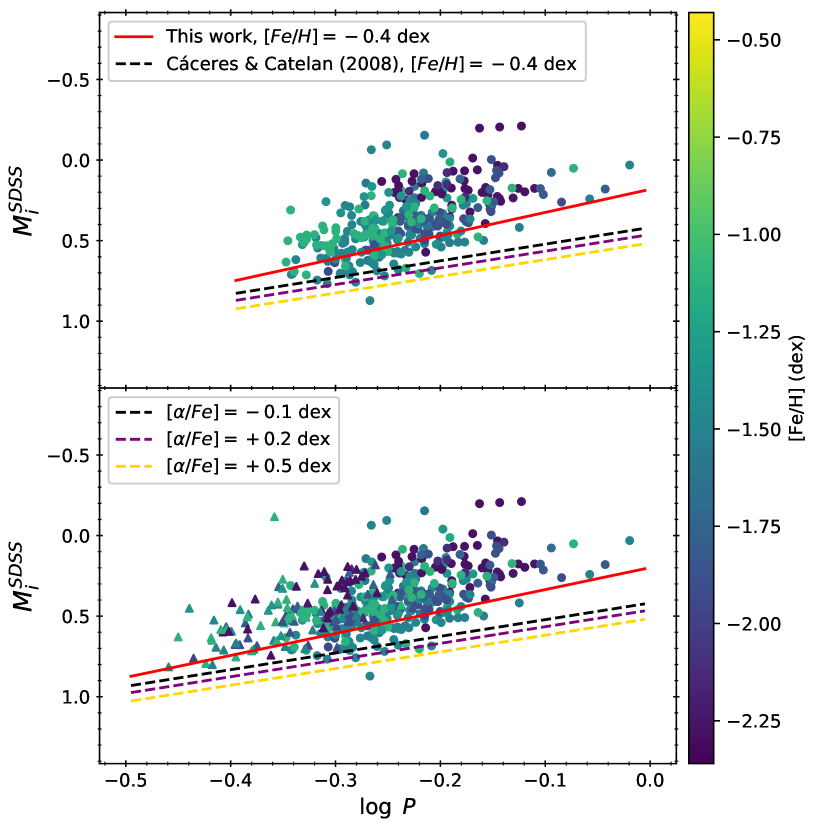
Figure 19: Comparison of the $i$-band PLZ relations given in Cáceres & Catelan (2008, as dashed lines) and our derived relations presented in Table 4 (in red solid lines), evaluated at $[\mathrm{Fe/H}]=-2.4$ dex (left panel) and $-0.4$ dex (right panel). For the theoretical PLZ relations, we also included the corresponding PLZ relations at three different adopted values of $[\alpha/\mathrm{Fe}]$ (see text for details). Note that the data points and our $i$-band PLZ relations have been transformed to the SDSS photometric system following the procedures described in Section 4.1. Top and bottom panels are for RR0 only, and RR0 and RR1 (after fundametalized the pulsation periods) combined samples, respectively.

Two theoretical investigations of PLZ relations in the SDSS photometric system were presented in Marconi et al. (2006) and Cáceres & Catelan (2008). Metallicity in these theoretical investigations were expressed as $\log Z$ instead of $[\mathrm{Fe/H}]$. Therefore, a $\log Z$-$[\mathrm{Fe/H}]$ conversion was taken from Cáceres & Catelan (2008, and reference therein) in the form of:

$$\log Z = \log(0.638\times 10^{[\alpha/\mathrm{Fe}]}+0.362)$$ (2)

$$+\mathrm{[Fe/H]}-1.765.$$

For globular clusters, $[\alpha/\mathrm{Fe}]$ varies between $\sim-0.1$ dex and $\sim+0.5$ dex (based on the compilation presented in Pritzl et al., 2005). Therefore, we adopted $[\alpha/\mathrm{Fe}]=-0.1$ and $+0.5$ dex, as well as the mid-point $+0.2$ dex, to construct the theoretical PLZ relation.

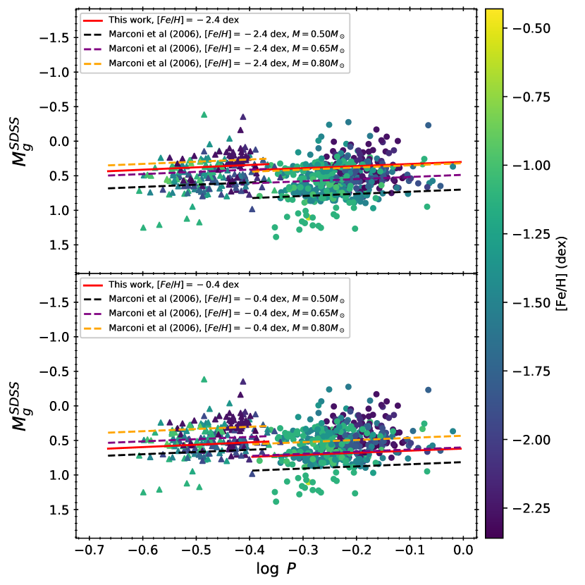
Figure 20: Comparison of the $g$-band PLZ relations given in Marconi et al. (2006, as dashed lines) and our derived relations presented in Table 4 (in red solid lines), evaluated at $[\mathrm{Fe/H}]=-2.4$ dex (top panel) and $-0.4$ dex (bottom panel), with a fixed $[\alpha/\mathrm{Fe}]=+0.2$ dex. For the semi-theoretical PLZ relations (see text for details), we also included the corresponding PLZ relations at three different adopted values of the mass $M$, covering the expected mass range for RR Lyrae. Note that the data points and our $g$-band PLZ relations have been transformed to the SDSS photometric system following the procedures described in Section 4.1. Circles and triangles represent the RR0 and RR1, respectively.

Cáceres & Catelan (2008) provided a simple $i$-band theoretical PLZ relation in the form of $M_{i}=0.908-1.035\log P+0.220\log Z$, this PLZ relation was compared to our derived PLZ relation in Figure 19 for the two adopted values of $[\mathrm{Fe/H}]$. Figure 19 revealed that slope of this theoretical $i$-band PLZ relation ($-1.035$) is shallower than the one we derived here ($-1.432\pm 0.144$ for RR0, or $-1.362\pm 0.093$ for RR0+RR1), or the one derived in Vivas et al. (2017, $-1.59\pm 0.09$ for RR0). Furthermore, the predicted $i$-band absolute magnitudes, using the theoretical and our derived PLZ relations, show a moderate agreement for RR Lyrae with periods between $\sim 0.5$ to $\sim 0.6$ days at low metallicity (i.e. $[\mathrm{Fe/H}]=-2.4$ dex). However, these two sets of PLZ relations are in disagreement when the metallicity is higher (as shown in right panel of Figure 19 with $[\mathrm{Fe/H}]=-0.4$ dex), due to the difference in the zero-point ($0.908$ vs. $-0.243\pm 0.055$) and the metallicity term ($0.220$ vs. $0.144\pm 0.018$) of the $i$-band PLZ relations in both studies. Cáceres & Catelan (2008) cautions the use of equation (2) for $Z>0.003$ (VandenBerg et al., 2000), corresponding to $[\mathrm{Fe/H}]=-0.9$ dex (at $[\alpha/\mathrm{Fe}]=+0.2$ dex). This might contribute to the disagreement at high metallicity.

From equation (2) and Figure 19, we note that the adopted value of $[\alpha/\mathrm{Fe}]$ only affects the zero-point of the PLZ relation. The difference on the PLZ zero-point between $[\alpha/\mathrm{Fe}]=-0.1$ and $+0.2$ dex is $c\times\Delta\log Z=-0.199c\sim\pm 0.044$ mag, and for $[\alpha/\mathrm{Fe}]=+0.2$ and $+0.5$ dex the difference is $c\times\Delta\log Z=-0.239c\sim\pm 0.053$ mag, at fixed $[\mathrm{Fe/H}]$, where $c=0.220$ is the metallicity term in the theoretical $i$-band PLZ relation from Cáceres & Catelan (2008). Hence, we adopted a single value of $[\alpha/\mathrm{Fe}]=+0.2$ dex throughout the rest of the paper.

The theoretical PLZ relations derived in Marconi et al. (2006) are available in the $ug$-band, with additional terms on colors and masses. We can only compare our PLZ relations to their $g$-band PLZ relations together with the $(g-r)$ and $(r-i)$ colors. We first realized that slopes of the theoretical $g$-band PLZ relations (Marconi et al., 2006) are steep: $-2.87$ and $\sim-3.1$ for the RR0 and RR1, respectively. These slopes are much steeper than those presented in Table 4 or in Vivas et al. (2017). However, the Marconi et al. (2006) PLZ relations also included a color term, and the colors for RR Lyrae are expected to follow a PC relation (for examples, see Section 5 and Cáceres & Catelan, 2008, for colors in the $gri$-band). Combining the derived period-color-metallicity (PCZ) relations from Section 5 (see Table 4) with theoretical PLZ relations from Marconi et al. (2006), we obtained the following semi-theoretical PLZ relations for the RR0:

$$M_{g} = 0.066-0.311\log P+0.117\mathrm{[Fe/H]}-1.87\log\frac{M}{M_{\odot}}$$ (4)

$$-0.06\log Z+3.35\delta_{c}\ \ \ \ [\mathrm{with\ (g-r)\ color}],$$

$$= -0.097-0.350\log P-0.003\mathrm{[Fe/H]}-1.94\log\frac{M}{M_{\odot}}$$

$$-0.024\log Z+2.27\delta_{c}\ \ \ \ [\mathrm{with\ (g-i)\ color}].$$

Slopes of these semi-theoretical relations are now closer to the empirical value given in Table 4 ($-0.302\pm 0.193$). Similarly, the semi-theoretical PLZ relations for the RR1 are:

$$M_{g} = -0.109-0.322\log P+0.061\mathrm{[Fe/H]}-1.63\log\frac{M}{M_{\odot}}$$ (6)

$$-0.042\log Z+3.57\delta_{c}\ \ \ \ [\mathrm{with\ (g-r)\ color}],$$

$$= 0.285+0.536\log P+0.033\mathrm{[Fe/H]}-1.72\log\frac{M}{M_{\odot}}$$

$$-0.017\log Z+2.334\delta_{c}\ \ \ \ [\mathrm{with\ (g-i)\ color}].$$

Slope given in equation (5) is closer to the empirical value of $-0.342\pm 0.289$. However, the slope found in equation (6) is drastically different, at which we do not have a formal explanation to account for this. Perhaps due to a much steeper slope for the RR1 $(g-i)$ PCZ relation. We will adopt equation (3) and (5) to be compared to our derived PLZ relations, because the slopes of these two semi-theoretical relations are closer to the empirical values. The $\delta_{c}$ in equation (3) to (6) is the correction term to covert the colors from Pan-STARRS1 photometric system to the SDSS photometric system, similar to the $\delta_{m}$ described in Section 4.1. The comparison is presented in Figure 20.

An additional mass term, $\log M/M_{\odot}$, was included in equation (3) and (5). Figure 20 reveals that this mass term has a larger impact on the zero-point of the PLZ relation, in contrast to the change of $[\alpha/\mathrm{Fe}]$ that affect the zero-point of the PLZ relation by a small amount ($\lesssim 0.05$ mag). At a fixed metallicity, the $g$-band semi-theoretical PLZ relations could be in agreement or in disagreement with our derived $g$-band PLZ relations depending on the adopted mass. For example, Figure 20 shows that at $[\mathrm{Fe/H}]=-2.4$ dex, these two sets of PLZ relation for RR0 agree when the mass is $\sim 0.8M_{\odot}$, but not for other lower masses. Similarly at $[\mathrm{Fe/H}]=-0.4$ dex, the RR0 semi-theoretical PLZ relations with mass of $\sim 0.65M_{\odot}$ are closer to the empirical PLZ relations given in Table 4.

5 The Period-Color-Metallicity Relations and the Color-Color Diagram

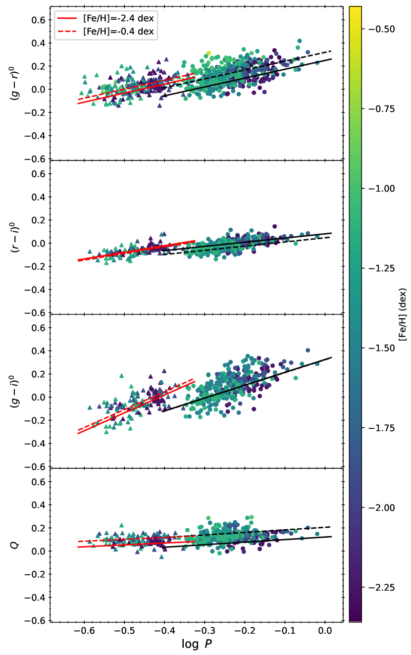
Figure 21: The extinction corrected PC relations (top three panels) and the extinction-free PQ relation (bottom panel) for our sample of RR Lyrae. The solid and dashed lines (in both red and black colors) represent the PCZ and PQZ relations evaluated at $[\mathrm{Fe/H}]=-2.4$ dex and $[\mathrm{Fe/H}]=-0.4$ dex, respectively. The relations for the combined sample of RR0 and RR1 (after fundametalized the periods) are similar, hence they are not included in this Figure.

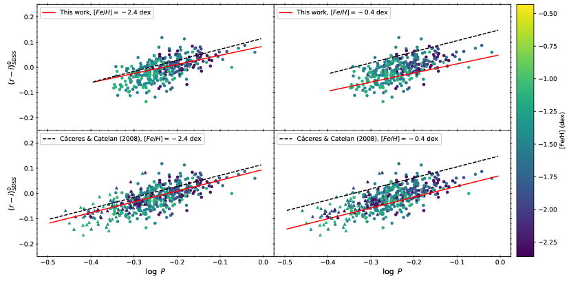
Figure 22: Comparison of the PCZ relations given in Cáceres & Catelan (2008, as dashed lines) and our derived relations presented in Table 4 (in red solid lines), evaluated at $[\mathrm{Fe/H}]=-2.4$ dex (left panels) and $-0.4$ dex (right panels), for the $(g-r)$ and the $(r-i)$ colors at the top and bottom panels, respectively. For the theoretical PLZ relations, we adopted a value of $[\alpha/\mathrm{Fe}]=+0.2$ dex (see text for details). Note that the data points and our PCZ relations have been transformed to the SDSS photometric system following the procedures described in Section 4.1. In each panels, the top and bottom sub-panels are for RR0 only, and RR0 and RR1 (after fundametalized the pulsation periods) combined samples, respectively.

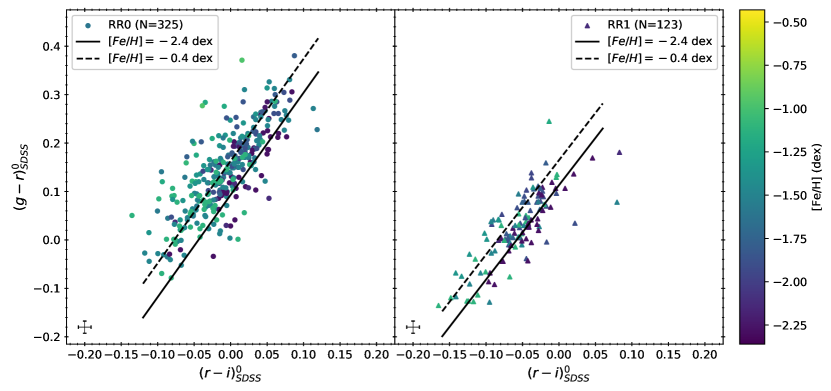
Figure 23: The extinction corrected color-color relations for RR0 (left panel) and RR1 (right panel) in our sample, where the mean magnitudes have been transformed to the SDSS system using the transformations provided in Tonry et al. (2012). Typical error bars of the colors are shown in the lower-left corners. Both the solid and dashed lines represent the theoretical color-color relations taken from Marconi et al. (2006) at a given metallicity (see text for more details).

We have fitted the extinction-corrected PCZ relations and the extinction-free PQZ relation with our sample of RR Lyrae, using equation (1) and the same methodology as described in Section 4. The fitted results are summarized in Table 4 and shown in Figure 21. We note that the metallicity terms for the PCZ and PQZ relations, the parameter $c$ in equation (1), in general are smaller than the PLZ and PWZ relations (except the $W^{gr}$ PWZ relations, see Section 4). For example, the metallicity term in $(r-i)$ PCZ relation for RR1 is consistent with zero. The $(g-i)$ PCZ relations have the steepest slopes and almost vanishing metallicity terms, for either RR0, RR1, or the combined sample of both. Dispersions of the PCZ and PQZ relations are also smaller, with $(r-i)$ PCZ relations have the smallest dispersion in all of the fitted relations.

Similar to the theoretical $i$-band PLZ relation, Cáceres & Catelan (2008) provided the theoretical PCZ relations in the $(g-r)$ and the $(r-i)$ colors. We compared their PCZ relations with those listed in Table 4, evaluated at two metallicities, as shown in Figure 22. These theoretical PCZ relations behave similar to the $i$-band PLZ relation (shown in Figure 19, see Section 4.2), such that they are in moderate agreement with our empirical relations at low metallicity, and in disagreement when the metallicity is high.

In addition to theoretical PLZ relations (see Section 4.2), Marconi et al. (2006) has also derived the metallicity-dependent color-color relations based on a series of pulsation models. In Figure 23, these theoretical color-color relations were shown as solid and dashed lines for the two adopted metallicity (see Section 4.2 for more details), together with the extinction-corrected colors for our sample of RR Lyrae. It can be seen from Figure 23 that the theoretical color-color relations trace a relatively narrow “stripe” in the color-color diagram, while the observed RR Lyrae show a much larger scatter along this stripe. As discussed in Marconi et al. (2006), several sources (both intrinsic and observational), in addition to metallicity, may contribute to the scatter seen in the color-color relations. This imply that the $(g-r)$ and $(r-i)$ color-color diagram is not a good diagnostic to discriminate metallicity for RR Lyrae.

6 An Example of Application: Distance to Dwarf Galaxy Crater II

Based on DECam observations, Vivas et al. (2020) identified 83 and 5 RR0 and RR1, respectively, in a dwarf galaxy Crater II. There is one RR0 (V24 identified in Joo et al., 2018), however, missed in Vivas et al. (2020) because it is located outside the footprint of DECam observations. This set of RR Lyrae provides an opportunity to compare and test various PL(Z) relations in a differential way. These include the empirical PL(Z) relations from Sesar et al. (2017), Vivas et al. (2017), Bhardwaj et al. (2021, by adopting the distance to M15 as listed in Table 2), and our results presented in Table 4. We excluded the theoretical $g$-band PLZ relation from Marconi et al. (2006) because of the mass-dependency, which has a significant impact on the zero-point of the PLZ relation (see discussion in Section 4.2). We also excluded the theoretical $i$-band PLZ relation from Cáceres & Catelan (2008), because Vivas et al. (2020) applied this relation to the RR Lyrae in Crater II, and found a distance modulus of $20.333\pm 0.004$ mag to this dwarf galaxy, by adopting $[\mathrm{Fe/H}]=-2.0$ dex and $[\alpha/\mathrm{Fe}]=+0.3$ dex.

Since the mean magnitudes of the observed RR Lyrae are available in the SDSS $gi$-band (Vivas et al., 2020) and lack of $r$-band data, same as in the case of Bhardwaj et al. (2021), making the transformation between various photometric systems non-trivial. We first transformed our RR Lyrae in the globular clusters to the SDSS photometric system, and a subset of these RR Lyrae with the same mean $(g-i)$ colors as the RR Lyrae in Crater II were used to determine the correction term, $\delta_{m}$, for the PLZ relations based on Pan-STARRS1 photometric system. These correction terms were found to be $0.040$ mag and $0.029$ mag in the $g$-band, and $-0.003$ mag and $-0.004$ mag in the $i$-band, where the first and the second numbers are for RR0 and RR1, respectively. In Table 6, we summarized the derived distance moduli ($\mu$) using the four mentioned empirical PL(Z) relations at $[\mathrm{Fe/H}]=-2.0$ dex, separately in the $g$- and $i$-band, while keeping the periods, mean magnitudes, and extinctions the same when fitting the PLZ relations to these RR Lyrae in Crater II.

Table 6: Distance moduli to Crater II derived with various PL(Z) relations, using $[\mathrm{Fe/H}]=-2.0$ dex.

PLZ Relations	RR0			RR1			RR0+RR1
	$\mu_{g}$	$\mu_{i}$	$\Delta\mu_{gi}$	$\mu_{g}$	$\mu_{i}$	$\Delta\mu_{gi}$	$\mu_{g}$	$\mu_{i}$	$\Delta\mu_{gi}$
This work (Table 4)	$20.488\pm 0.006$	$20.427\pm 0.004$	0.061	$20.465\pm 0.016$	$20.406\pm 0.014$	0.059	$20.450\pm 0.006$	$20.375\pm 0.004$	0.075
Vivas et al. (2017)	$20.374\pm 0.006$	$20.277\pm 0.005$	0.097	$20.396\pm 0.017$	$20.287\pm 0.014$	0.109	$\cdots$	$\cdots$	$\cdots$
Sesar et al. (2017)	$20.262\pm 0.008$	$20.287\pm 0.005$	-0.025	$\cdots$	$\cdots$	$\cdots$	$\cdots$	$\cdots$	$\cdots$
Bhardwaj et al. (2021)	$20.494\pm 0.006$	$20.452\pm 0.004$	0.042	$20.475\pm 0.017$	$20.433\pm 0.015$	0.042	$20.506\pm 0.006$	$20.455\pm 0.004$	0.051

Note. — $\Delta\mu_{gi}=\mu_{g}-\mu_{i}$ is the difference of the distance moduli in the $g$- and $i$-band. Errors on each of the distance moduli are random errors only.

Table 7: Same as Table 6, but with reddening values from the Bayerstar2019 3D reddening map.

PLZ Relations	RR0			RR1			RR0+RR1
	$\mu_{g}$	$\mu_{i}$	$\Delta\mu_{gi}$	$\mu_{g}$	$\mu_{i}$	$\Delta\mu_{gi}$	$\mu_{g}$	$\mu_{i}$	$\Delta\mu_{gi}$
This work (Table 4)	$20.426\pm 0.007$	$20.395\pm 0.005$	0.031	$20.393\pm 0.016$	$20.369\pm 0.012$	0.024	$20.387\pm 0.007$	$20.343\pm 0.005$	0.044
Vivas et al. (2017)	$20.312\pm 0.008$	$20.245\pm 0.005$	0.067	$20.325\pm 0.014$	$20.250\pm 0.013$	0.075	$\cdots$	$\cdots$	$\cdots$
Sesar et al. (2017)	$20.200\pm 0.009$	$20.255\pm 0.005$	-0.055	$\cdots$	$\cdots$	$\cdots$	$\cdots$	$\cdots$	$\cdots$
Bhardwaj et al. (2021)	$20.432\pm 0.007$	$20.420\pm 0.005$	0.012	$20.404\pm 0.019$	$20.396\pm 0.015$	0.008	$20.444\pm 0.007$	$20.423\pm 0.005$	0.021

Note. — $\Delta\mu_{gi}=\mu_{g}-\mu_{i}$ is the difference of the distance moduli in the $g$- and $i$-band. Errors on each of the distance moduli are random errors only.

Table 6 reveals that the derived distance moduli are in general larger than $20.333$ mag as determined in Vivas et al. (2020), except the Sesar et al. (2017) PLZ relations and the $i$-band PL relations from Vivas et al. (2017). To bring the distance moduli fitted from other PL(Z) relations closer to $20.333$ mag, the metallicity of Crater II has to increase. For the two sets of PL relations without the metallicity term, we note that Bhardwaj et al. (2021) PL relations give a larger distance modulus than the PL relations derived in Vivas et al. (2017). The Bhardwaj et al. (2021) and Vivas et al. (2017) PL relations were derived using RR Lyrae in M15 and M5, respectively, at which is M15 is more metal-poor than M5, hence the Bhardwaj et al. (2021) PL relations should be favored to be applied to RR Lyrae in Crater II (assuming its metallicity of $[\mathrm{Fe/H}]=-2.0$ dex is correct). Therefore, either the true distance modulus to Crater II is larger (than $20.333$ mag) or its metallicity is higher (than $-2.0$ dex), or both.

Since the mean magnitudes have been corrected for extinction, we expect the $g$- and $i$-band distance moduli should be roughly the same, or $\Delta\mu_{gi}=\mu_{g}-\mu_{i}\sim 0$. Except for distance moduli fitted with Sesar et al. (2017) PLZ relations (presumably due to the problem in $g$-band, see Section 4.1), we found that the $g$-band distance moduli are larger than their counterparts in the $i$-band (Table 6). One possibility is the slight incorrect estimation of extinction adopted in Vivas et al. (2017). Instead of using the $E(B-V)$ values provided in Vivas et al. (2017), we use the same Bayerstar2019 3D reddening map as described in Section 2.2 to correct the extinction for the $gi$-band mean magnitudes. The fitted distance moduli are given in Table 7. Again with the exception of distance moduli based on Sesar et al. (2017) PLZ relations, now the $gi$-band distance moduli are closer to each others. Vivas et al. (2017) PL relations give the largest $\Delta\mu_{gi}$, indicating an extra metallicity term is needed to be applied to the derived distance moduli, because the Vivas et al. (2017) PL relations are based on RR Lyrae in M5, which has a higher metallicity than the assumed metallicity for Crater II. We note that $\Delta\mu_{gi}$ from using our PLZ relations (Table 4) are larger than those using the PL relations from Bhardwaj et al. (2021), possibly due to the photometric transformation because without the photometric transformation, the $\Delta\mu_{gi}$ using our PLZ relations are even larger. Since by definition the difference of the distance moduli in two filters is also a measure of extinction (for examples, see Kelson et al., 1996; Turner et al., 1998; Freedman et al., 2001), and the foreground extinctions have been corrected using the Bayerstar2019 3D reddening map, we suggest the excess of $\Delta\mu_{gi}$ is due to the internal extinction of Crater II, that is $\Delta_{gi}=(\mu_{g}+A_{g})-(\mu_{i}+A_{i})=E(g-i)\sim 0.03$ or $\sim 0.01$ mag depending on the adopted PL(Z) relations given in Table 4 or Bhardwaj et al. (2021).

Since there should only have one distance modulus ($\mu_{0}$) to Crater II, it is possible to simultaneously fit four PLZ relations, the $gi$-band PLZ relations for both RR0 and RR1, to the data by defining the following merit function:

$$\chi^{2} = \sum_{j=1}^{N_{\lambda,\psi}}\sum_{\lambda=\{g,i\}}\sum_{\psi=\{0,1\}}\frac{(m^{j}_{\lambda,\psi}-M^{j}_{\lambda,\psi}-\mu_{0})^{2}}{\sigma^{2}_{\lambda,\psi}}$$ (7)

$$\mathrm{where} \ M^{j}_{\lambda,\psi}=a_{\lambda,\psi}+b_{\lambda,\psi}\log P^{j}_{\lambda,\psi}+c_{\lambda,\psi}\mathrm{[Fe/H]}.$$

In above equation, $\lambda$ represents the filters (either $g$ or $i$), and $\psi$ represents pulsation modes (either $0$ or $1$). Parameters $a$, $b$, and $c$ are same as the PLZ relation defined in equation (1), and $\sigma$ is the dispersion of the respected PLZ relation. Adopting $\mathrm{[Fe/H]}=-2.0$ dex and using the values given in Table 4 for our derived PLZ relations, we obtained $\mu_{0}=20.361\pm 0.004$ mag (random error only) after including the additional correction of internal extinction of Crater II, $E(g-i)\sim 0.03$ mag, to the data. Allowing $\mathrm{[Fe/H]}$ as another free parameter to be fitted, we derived $\mu_{0}=20.327\pm 0.100$ mag and $\mathrm{[Fe/H]}=-1.76\pm 0.69$ dex using the ordinary least squares (OLS) regression. As a sanity check, we have also derived the distance modulus to Crater II using the $W^{gi}$ PWZ relations, evaluated at $\mathrm{[Fe/H]}=-2.0$ dex. After transforming our PWZ relations to SDSS photometric system, and using $W^{gi}_{SDSS}=g_{SDSS}-2.058(g_{SDSS}-i_{SDSS})$, we obtained $\mu_{0}=20.354\pm 0.004$ mag (random error only) by simultaneous fitting the RR0 and RR1 sample with equation (7). Since multiple transformations were involved for the Wesenheit index $W^{gi}$, we adopted our derived distance modulus based on the PLZ relations instead of the PWZ relations.

We recall that in general a more metal-poor system would imply a larger distance modulus due to the positive metallicity term, the parameter $c$ in equation (1), in the PLZ relation. Our results are consistent with this expectation ($\mu_{0}=20.361$ mag at $\mathrm{[Fe/H]}=-2.0$ dex vs. $\mu_{0}=20.327$ mag at $\mathrm{[Fe/H]}=-1.76$ dex). Clearly, there is a degeneracy, or correlation, between $\mu_{0}$ and $\mathrm{[Fe/H]}$. Therefore, instead of using OLS regression, we fit equation (7) using technique of Bayesian linear regression to the data. We adopted a flat (uniform) prior on both $\mu_{0}$ (between 10 and 30) and $\mathrm{[Fe/H]}$ (between $-2.5$ and $-0.5$), and the affine-invariant Markov Chain Monte Carlo sampler package emcee (Foreman-Mackey et al., 2013) was used to sample the posterior distribution. The result is shown in Figure 24, produced from the corner package (Foreman-Mackey, 2016), at which the (anti-)correlation of these two parameters can be clearly seen. By adopting median as the estimator of the parameters, we found the following best-fit values: $\mu_{0}=20.313_{-0.083}^{+0.074}$ mag, and $\mathrm{[Fe/H]}=-1.67_{-0.51}^{+0.58}$ dex, where the error-bars represent the $16^{\mathrm{th}}$ and $84^{\mathrm{th}}$ percentiles of the distributions.

Nevertheless, metallicity of Crater II has been measured to be around $-2.0$ dex from multiple studies (Torrealba et al., 2016; Caldwell et al., 2017; Fu et al., 2019; Walker et al., 2019), and unlikely to have a higher metallicity around $-1.7$ dex. Therefore, the true distance modulus of Crater II should be larger than $20.333$ mag as reported in Vivas et al. (2020).

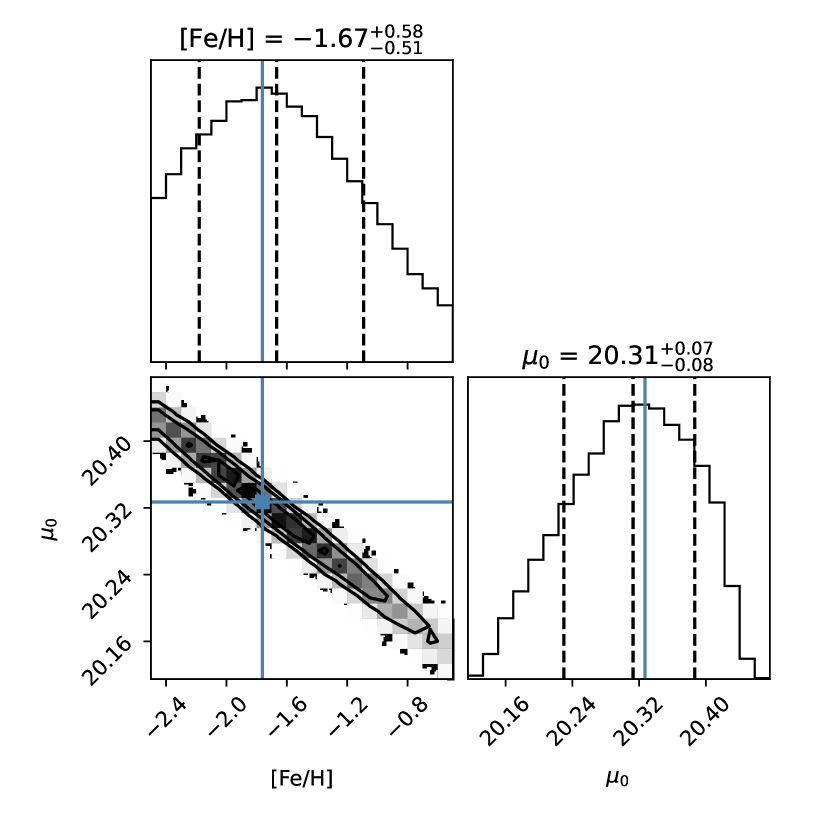
Figure 24: The corner plot based on the emcee sampling on the posterior distributions for $\mu_{0}$ and $\mathrm{[Fe/H]}$, the sampling was run with 128 walkers for 10000 steps. The vertical dashed lines on the histograms represent the $16^{\mathrm{th}}$, $50^{\mathrm{th}}$, and $84^{\mathrm{th}}$ percentiles of the distributions. The blue lines marked the results obtained from the OLS regression.

7 Conclusion

In this work, we derived the $gri$-band PLZ and PWZ relations, in the Pan-STARRS1 photometric system, based on $\sim 750$ RR Lyrae located in 46 globular clusters. These PLZ and PWZ relations were derived as homogeneous as possible, such as only using the light curves data from ZTF, correcting the extinction using the same Bayerstar2019 3D reddening map, and adopted the same sources for the metallicity and distances from the GOTHAM survey and Baumgardt & Vasiliev (2021), respectively. Table 4 presents the fitted results for these PLZ and PWZ relations. Other results obtained in this work are summarized as follow.

1. Based on our simulations, we found that the derived mean magnitudes may not be reliable or accurate with template light curve fitting approach when the light curve has a smaller number of data points. We recommend only fitting the observed light curves with 10 or more data points for deriving the mean magnitudes. We have also derived an empirical fitting equation to estimate the errors on the fitted mean magnitudes.

2. Given that blending is unavoidable for RR Lyrae located in globular clusters, we applied several selection criteria to exclude RR Lyrae that might affected by blending, as well as other RR Lyrae with problematic light curves. These selection criteria utilized information based on amplitudes, amplitudes ratios, colors, and/or residuals from the PL and PW relations. In case of the PL/PW residuals, we found there are indications that for RR Lyrae with brighter mean magnitudes (than expected) they also tend to have smaller amplitudes, strongly indicating the presence of blending.

3. We notice the $W^{gr}$ PWZ relations exhibit very weak metallicity dependence, similar to the theoretical PW relations constructed in $BVR$-band (Marconi et al., 2015). We also notice the PLZ and PWZ relations involving $i$-band show the smallest dispersions, therefore increasing the $i$-band ZTF observations in the near future would be beneficial.

4. Compared to the literature PL(Z) relations, we found that our PLZ relations disagree with those presented in Sesar et al. (2017, especially in the $g$-band), but in very good agreement with the PL relations derived in Vivas et al. (2017). In comparison to Bhardwaj et al. (2021) $gi$-band PL relations, we found a fairly good agreement, although our PL(Z) relations are fainter in the $i$-band for the RR1 and RR0+RR1 sample.

5. The theoretical $i$-band PLZ relation derived in Cáceres & Catelan (2008) was comparable to our derived PLZ relation at low metallicity ($\mathrm{[Fe/H]}=-2.4$ dex). However, disagreement was found for these two sets of $i$-band PLZ relation at high metallicity ($\mathrm{[Fe/H]}=-0.4$ dex), presumably due to invalid $\log Z$-$\mathrm{[Fe/H]}$ conversion at high metallicity.

6. The comparison to the theoretical PLZ relations presented in Marconi et al. (2006) was more complicated due to the inclusion of colors and mass terms in the theoretical relations. To eliminate the color term, we substituted our derived PCZ relations to the theoretical relations, and obtained semi-theoretical period-luminosity-metallicity-mass relations. The mass term in these relations has a non-negligible impact on the zero-point of the corresponding PLZ relation.

7. In addition to PLZ and PWZ relations, we have also derived the PCZ and PQZ relations with our sample of RR Lyrae in globular clusters. Again, our empirical PCZ relations are in moderate agreement with the theoretical PCZ relations (Cáceres & Catelan, 2008) at low metallicity but not at the high metallicity, probably due to same reason(s) as in the case of $i$-band PLZ relation.

8. The empirical color-color diagram shows a larger scatter than the theoretical color-color relations at various metallicities. This implies the $(g-r)$ and $(r-i)$ color-color diagram is not a good diagnostic for determining the metallicity for RR Lyrae.

9. We applied the empirical PL(Z) relations to RR Lyrae found in a dwarf galaxy Crater II. Using published data, we found that the derived distance modulus to Crater II is in general larger than $20.333$ mag (Vivas et al., 2020). Further analysis revealed that Crater II needs to be more metal-rich in order to bring the distance modulus derived using our PLZ relations closer to the published values, or Crater II is indeed located in a further distance. Based on our analysis, we suggested Crater II may have internal extinction of $E(g-i)\sim 0.01$ or $\sim 0.03$ mag.

Our derived PLZ and PWZ relations in $gri$-band would be beneficial for various distance scale applications. For examples, precise distance can be derived to faint RR Lyrae located in outer Galactic halo or newly discovered (ultra-faint or diffuse) dwarf galaxies, such as those discovered from the HyperSuprime-Cam Subaru Strategic Program (HSC-SSP, Aihara et al., 2018) in northern sky and the Vera Rubin Observatory Legacy Survey of Space and Time (LSST, Ivezić et al., 2019) in southern sky, as well as other similar optical surveys. This in turn is of great interest for the study of sub-structure in our Galactic halo (for examples, see Lancaster et al., 2019). At present RR Lyrae observations are possible up to $\sim 2$ Mpc distance (Da Costa et al., 2010), just slightly beyond the Local Group, and we anticipated new dwarf galaxies will be routinely discovered in various optical surveys (such as HSC-SSP and/or LSST), an example is Eridanus IV recently reported in Cerny et al. (2021).

References

- Abbott et al. (2021) Abbott, T. M. C., Adamów, M., Aguena, M., et al. 2021, ApJS, 255, 20
- Aihara et al. (2018) Aihara, H., Arimoto, N., Armstrong, R., et al. 2018, PASJ, 70, S4
- Astropy Collaboration et al. (2013) Astropy Collaboration, Robitaille, T. P., Tollerud, E. J., et al. 2013, A&A, 558, A33
- Astropy Collaboration et al. (2018) Astropy Collaboration, Price-Whelan, A. M., Sipőcz, B. M., et al. 2018, AJ, 156, 123
- Baumgardt & Vasiliev (2021) Baumgardt, H. & Vasiliev, E. 2021, MNRAS, 505, 5957
- Beaton et al. (2018) Beaton, R. L., Bono, G., Braga, V. F., et al. 2018, Space Sci. Rev., 214, 113
- Bellm & Kulkarni (2017) Bellm, E. & Kulkarni, S. 2017, Nature Astronomy, 1, 0071
- Bellm et al. (2019) Bellm, E. C., Kulkarni, S. R., Graham, M. J., et al. 2019, PASP, 131, 018002
- Benkő et al. (2006) Benkő, J. M., Bakos, G. Á., & Nuspl, J. 2006, MNRAS, 372, 1657
- Bhardwaj (2020) Bhardwaj, A. 2020, Journal of Astrophysics and Astronomy, 41, 23
- Bhardwaj (2022) Bhardwaj, A. B. 2022, Universe, 8, 122
- Bhardwaj et al. (2016) Bhardwaj, A., Kanbur, S. M., Macri, L. M., et al. 2016, AJ, 151, 88
- Bhardwaj et al. (2020) Bhardwaj, A., Rejkuba, M., de Grijs, R., et al. 2020, AJ, 160, 220
- Bhardwaj et al. (2021) Bhardwaj, A., Rejkuba, M., Sloan, G. C., et al. 2021, ApJ, 922, 20
- Bono (2003) Bono, G. 2003, Stellar Candles for the Extragalactic Distance Scale, edited by D. Alloin & W. Gieren, Lecture Notes in Physics, 635:85
- Bono et al. (2001) Bono, G., Caputo, F., Castellani, V., et al. 2001, MNRAS, 326, 1183
- Bono et al. (2003) Bono, G., Caputo, F., Castellani, V., et al. 2003, MNRAS, 344, 1097
- Bono et al. (2016) Bono, G., Braga, V. F., Pietrinferni, A., et al. 2016, Mem. Soc. Astron. Italiana, 87, 358
- Borissova et al. (2007) Borissova, J., Ivanov, V. D., Stephens, A. W., et al. 2007, A&A, 474, 121
- Braga et al. (2016) Braga, V. F., Stetson, P. B., Bono, G., et al. 2016, AJ, 152
- Caldwell et al. (2017) Caldwell, N., Walker, M. G., Mateo, M., et al. 2017, ApJ, 839, 20
- Cardiel (2009) Cardiel, N. 2009, MNRAS, 396, 680
- Catelan et al. (2004) Catelan, M., Pritzl, B. J., & Smith, H. A. 2004, ApJS, 154, 633
- Cáceres & Catelan (2008) Cáceres, C. & Catelan, M. 2008, ApJS, 179, 242
- Cerny et al. (2021) Cerny, W., Pace, A. B., Drlica-Wagner, A., et al. 2021, ApJ, 920, L44
- Chambers et al. (2016) Chambers, K. C., Magnier, E. A., Metcalfe, N., et al. 2016, arXiv:1612.05560
- Chicherov (1997) Chicherov, A. V. 1997, Astronomy Letters, 23, 600
- Clement et al. (2001) Clement, C. M., Muzzin, A., Dufton, Q., et al. 2001, AJ, 122, 2587
- Clement (2017) Clement, C. M. 2017, VizieR Online Data Catalog, V/150
- Coppola et al. (2015) Coppola, G., Marconi, M., Stetson, P. B., et al. 2015, ApJ, 814, 71
- Corwin & Carney (2001) Corwin, T. M. & Carney, B. W. 2001, AJ, 122, 3183
- Da Costa et al. (2010) Da Costa, G. S., Rejkuba, M., Jerjen, H., et al. 2010, ApJ, 708, L121
- Dambis et al. (2014) Dambis, A. K., Rastorguev, A. S., & Zabolotskikh, M. V. 2014, MNRAS, 439, 3765
- Dark Energy Survey Collaboration et al. (2016) Dark Energy Survey Collaboration, Abbott, T., Abdalla, F. B., et al. 2016, MNRAS, 460, 1270.
- Dekany et al. (2020) Dekany, R., Smith, R. M., Riddle, R., et al. 2020, PASP, 132, 038001
- Dias et al. (2015) Dias, B., Barbuy, B., Saviane, I., et al. 2015, A&A, 573, A13
- Dias et al. (2016a) Dias, B., Barbuy, B., Saviane, I., et al. 2016a, A&A, 590, A9
- Dias et al. (2016b) Dias, B., Saviane, I., Barbuy, B., et al. 2016b, The Messenger, 165, 19
- Drake et al. (2013) Drake, A. J., Catelan, M., Djorgovski, S. G., et al. 2013, ApJ, 763, 32
- Flaugher et al. (2015) Flaugher, B., Diehl, H. T., Honscheid, K., et al. 2015, AJ, 150, 150
- Foreman-Mackey (2016) Foreman-Mackey, D. 2016, The Journal of Open Source Software, 1, 24
- Foreman-Mackey et al. (2013) Foreman-Mackey, D., Hogg, D. W., Lang, D., et al. 2013, PASP, 125, 306
- Freedman et al. (2001) Freedman, W. L., Madore, B. F., Gibson, B. K., et al. 2001, ApJ, 553, 47
- Fu et al. (2019) Fu, S. W., Simon, J. D., & Alarcón Jara, A. G. 2019, ApJ, 883, 11
- Graham et al. (2019) Graham, M. J., Kulkarni, S. R., Bellm, E. C., et al. 2019, PASP, 131, 078001
- Green (2018) Green, G. M. 2018, The Journal of Open Source Software, 3, 695
- Green et al. (2019) Green, G. M., Schlafly, E., Zucker, C., et al. 2019, ApJ, 887, 93
- Guhathakurta et al. (1994) Guhathakurta, P., Yanny, B., Bahcall, J. N., et al. 1994, AJ, 108, 1786
- Harris et al. (2020) Harris, C. R., Millman, K. J., van der Walt, S. J., et al. 2020, Nature, 585, 357
- Heinze et al. (2018) Heinze, A. N., Tonry, J. L., Denneau, L., et al. 2018, AJ, 156, 241
- Hunter (2007) Hunter, J. D. 2007, Computing in Science and Engineering, 9, 90
- Iben (1974) Iben, I. 1974, ARA&A, 12, 215
- Ivezić et al. (2019) Ivezić, Ž., Kahn, S. M., Tyson, J. A., et al. 2019, ApJ, 873, 111
- Joo et al. (2018) Joo, S.-J., Kyeong, J., Yang, S.-C., et al. 2018, ApJ, 861, 23
- Kelson et al. (1996) Kelson, D. D., Illingworth, G. D., Freedman, W. F., et al. 1996, ApJ, 463, 26
- Kochanek et al. (2017) Kochanek, C. S., Shappee, B. J., Stanek, K. Z., et al. 2017, PASP, 129, 104502
- Kopacki (2013) Kopacki, G. 2013, Acta Astronomica, 63, 91
- Kunder et al. (2013) Kunder, A., Stetson, P. B., Cassisi, S., et al. 2013, AJ, 146, 119
- Lancaster et al. (2019) Lancaster, L., Belokurov, V., & Evans, N. W. 2019, MNRAS, 484, 2556
- Madore (1982) Madore, B. F. 1982, ApJ, 253, 575
- Madore & Freedman (1991) Madore, B. F. & Freedman, W. L. 1991, PASP, 103, 933
- Magnier et al. (2020) Magnier, E. A., Sweeney, W. E., Chambers, K. C., et al. 2020, ApJS, 251, 5
- Marconi et al. (2003) Marconi, M., Caputo, F., Di Criscienzo, M., et al. 2003, ApJ, 596, 299
- Marconi et al. (2006) Marconi, M., Cignoni, M., Di Criscienzo, M., et al. 2006, MNRAS, 371, 1503
- Marconi et al. (2015) Marconi, M., Coppola, G., Bono, G., et al. 2015, ApJ, 808, 50
- Masci et al. (2019) Masci, F. J., Laher, R. R., Rusholme, B., et al. 2019, PASP, 131, 018003
- Muraveva et al. (2018) Muraveva, T., Delgado, H. E., Clementini, G., et al. 2018, MNRAS, 481, 1195
- Neeley et al. (2017) Neeley, J. R., Marengo, M., Bono, G., et al. 2017, ApJ, 841, 84
- Neeley et al. (2019) Neeley, J. R., Marengo, M., Freedman, W. L., et al. 2019, MNRAS, 490, 4254
- Nemec et al. (1994) Nemec, J. M., Nemec, A. F. L., & Lutz, T. E. 1994, AJ, 108, 222
- Ngeow et al. (2021) Ngeow, C.-C., Liao, S.-H., Bellm, E. C., et al. 2021, AJ, 162, 63
- Pollacco et al. (2006) Pollacco, D. L., Skillen, I., Collier Cameron, A., et al. 2006, PASP, 118, 1407
- Pritzl et al. (2005) Pritzl, B. J., Venn, K. A., & Irwin, M. 2005, AJ, 130, 2140
- Riess et al. (2020) Riess, A. G., Yuan, W., Casertano, S., et al. 2020, ApJ, 896, L43
- Sandage & Tammann (2006) Sandage, A. & Tammann, G. A. 2006, ARA&A, 44, 93
- Sesar et al. (2010) Sesar, B., Ivezić, Ž., Grammer, S. H., et al. 2010, ApJ, 708, 717
- Sesar et al. (2011) Sesar, B., Stuart, J. S., Ivezić, Ž., et al. 2011, AJ, 142, 190
- Sesar et al. (2017) Sesar, B., Hernitschek, N., Mitrović, S., et al. 2017, AJ, 153, 204
- Smith (2004) Smith, H. A. 2004, RR Lyrae Stars, by Horace A. Smith, pp. 166. ISBN 0521548179. Cambridge, UK: Cambridge University Press, September 2004
- Sollima et al. (2006) Sollima, A., Cacciari, C., & Valenti, E. 2006, MNRAS, 372, 1675
- Tonry et al. (2012) Tonry, J. L., Stubbs, C. W., Lykke, K. R., et al. 2012, ApJ, 750, 99
- Tonry et al. (2018) Tonry, J. L., Denneau, L., Heinze, A. N., et al. 2018, PASP, 130, 064505
- Torrealba et al. (2016) Torrealba, G., Koposov, S. E., Belokurov, V., et al. 2016, MNRAS, 459, 2370
- Turner et al. (1998) Turner, A., Ferrarese, L., Saha, A., et al. 1998, ApJ, 505, 207
- VandenBerg et al. (2000) VandenBerg, D. A., Swenson, F. J., Rogers, F. J., et al. 2000, ApJ, 532, 430
- VanderPlas & Ivezić (2015) VanderPlas, J. T., & Ivezić, Ž. 2015, ApJ, 812, 18
- VanderPlas (2016) VanderPlas, J. 2016, gatspy: General tools for Astronomical Time Series in Python, ascl:1610.007
- Vásquez et al. (2018) Vásquez, S., Saviane, I., Held, E. V., et al. 2018, A&A, 619, A13
- Virtanen et al. (2020) Virtanen, P., Gommers, R., Oliphant, T. E., et al. 2020, Nature Methods, 17, 261
- Vivas et al. (2017) Vivas, A. K., Saha, A., Olsen, K., et al. 2017, AJ, 154, 85
- Vivas et al. (2020) Vivas, A. K., Walker, A. R., Martínez-Vázquez, C. E., et al. 2020, MNRAS, 492, 1061
- Walker et al. (2019) Walker, A. R., Martínez-Vázquez, C. E., Monelli, M., et al. 2019, MNRAS, 490, 4121