Detectable gravitational waves from preheating probes nonthermal dark matter
Abstract
We describe the challenges and pathways when probing inflaton as dark matter with the stochastic gravitational waves (GWs) signal generated during the (p)reheating. Such scenarios are of utmost interest when no other interaction between the visible and dark sectors is present, therefore having no other detectability prospects. We consider the remnant energy in the coherently oscillating inflaton’s zeroth mode to contribute to the observed relic dark matter density in the Universe. To fully capture the nonlinear dynamics and the effects of back-reactions during the oscillation, we resort to full nonlinear lattice simulation with pseudo-spectral methods to eliminate the differencing noises. We investigate for models whose behavior during the reheating era is of type and find the typical primordial stochastic GWs backgrounds spectrum from scatterings among highly populated inflaton modes behaving like matter. We comment on the challenges of constructing such viable inflationary models such that the inflaton will account for the total dark matter of the universe while the produced GWs are within the future GWs detectors such as BBO, DECIGO, PTA, AION-MAGIS, and CE. We also describe the necessary modifications to the standard perturbative reheating scenario to prevent the depletion of residual inflaton energy via perturbative decay
I Introduction
The origin and composition of dark matter (DM) in the Universe remains an open problem in modern particle physics and cosmology Jungman:1995df ; Bertone:2004pz ; Feng:2010gw . Even with great experimental efforts over the last 30 years, no clinching evidence of the existence of thermal frozen out DM dubbed as the famous “WIMP miracle” Lee:1977ua ; Scherrer:1985zt ; Srednicki:1988ce ; Gondolo:1990dk has been found in any DM search experiments PandaX-II:2017hlx ; PandaX:2018wtu ; XENON:2020kmp ; XENON:2018voc ; LUX-ZEPLIN:2018poe ; DARWIN:2016hyl , or via indirect detection HESS:2016mib ; MAGIC:2016xys or through collider physics searches (e.g. at the LHC ATLAS:2017bfj ; CMS:2017zts ). This motivates us to consider alternative DM production, particularly nonthermal production mechanisms, such that the observed DM abundance is generated out of equilibrium by the so-called freeze-in mechanism McDonald:2001vt ; Hall:2009bx ; Bernal:2017kxu , or say, via particle production during (p)-reheating Moroi:1994rs ; Kawasaki:1995cy ; Moroi:1999zb ; Jeong:2011sg ; Ellis:2015jpg ; Harigaya:2014waa ; Garcia:2018wtq ; Harigaya:2019tzu ; Garcia:2020eof ; Chung:1998zb ; Chung:1998ua ; Co:2017mop .
Interestingly, irrespective of the production mechanisms, the expected signals and constraints on the dark matter candidates are dictated by their interactions with the states of the standard model (SM). In this paper, we consider the scenario in which the DM relic abundance is set via the inflaton oscillations and decay, which is similar to the out-of-equilibrium freeze-in production mechanism. The cosmic inflation resolves the flatness and horizon problem and seeds the initial density fluctuations for large-scale structure formation Brout:1977ix ; Sato:1980yn ; Guth:1980zm ; Linde:1981mu ; Starobinsky:1982ee , and is considered to be driven by a neutral scalar field — stable on cosmological scales — can also be a natural dark matter candidate. Several such possibilities have been considered in the literature so far Liddle:2006qz ; Cardenas:2007xh ; Panotopoulos:2007ri ; Liddle:2008bm ; Bose:2009kc ; Lerner:2009xg ; DeSantiago:2011qb ; Khoze:2013uia ; Mukaida:2014kpa ; Fairbairn:2014zta ; Bastero-Gil:2015lga ; Kahlhoefer:2015jma ; Tenkanen:2016twd ; Daido:2017wwb ; Choubey:2017hsq ; Daido:2017tbr ; Hooper:2018buz ; Borah:2018rca ; Manso:2018cba ; Rosa:2018iff ; Almeida:2018oid . Generation of dark matter in the primordial Universe can be due to the incomplete decay of the inflaton (the remnant inflaton as the DM) or from the decaying inflaton — producing DM along with other SM degrees of freedom. The fact that only one scalar field can minimally explain both inflation (explaining the temperature fluctuations as seen in the cosmic microwave background radiation (CMB) Aghanim:2018eyx ) and make up the currently observed DM abundance in the Universe, is needless to say, an economical idea worth our attention.
However, such a nonthermal production of dark matter is impossible to detect222Such non-thermal particle production was proposed to be tested via dark radiation or measurements during Big Bang Nucleosynthesis (BBN) & CMB era, in context to neutrino anomalies Paul:2018njm . in any conventional astrophysical or laboratory-based dark matter searches, as they do not communicate with the visible sector (SM) and are typically considered to be beyond the paradigm of testability via any other interactions. Thankfully, the gravitational waves generated during the nonlinear preheating phase after inflation can provide an alternative channel for DM searches.
The initial phase of inflationary (p)-reheating (see, e.g., Refs. Kofman:1994rk ; Kofman:1997yn ; Mukaida:2013xxa ) is marked by resonant growth of the inflaton fluctuations and other fields that are coupled to the inflaton. The preheating soon gives rise to large inhomogeneties in the field fluctuations. These inhomogeneities act as a source of classical stochastic background gravitational waves (SGWB) Khlebnikov:1997di ; Easther:2006gt . The production of such SGWB signals has been studied in literature over the years in various contexts such as single-field chaotic inflation Easther:2006gt ; Easther:2006vd ; Easther:2007vj ; Dufaux:2007pt , preheating after hybrid inflation Garcia-Bellido:2007nns ; Garcia-Bellido:2007fiu ; Dufaux:2008dn ; Ringwald:2022xif , including production of gauge fields during preheating Dufaux:2010cf ; Adshead:2018doq ; Adshead:2019lbr , and for GWs production from oscillons from inflationary potentials that ‘opens up’ away from the minimum Antusch:2016con ; Amin:2018xfe ; Lozanov:2019ylm .
Inspired by the considerations mentioned above, this study addresses the issue of inflaton as dark matter, with a focus on the possibility of detection of the GW signals generated during the preheating phase. Our findings reveal that, with specific parameter choices, these GWs produced during preheating can be observable through GW detectors such as DECIGO, BBO, CE, and ET. Additionally, when exploring the inflaton as a candidate for dark matter, it places constraints on the parameter space of the inflaton coupling to fields. The significance of these alternative probes cannot be overstated, especially in contrast to traditional dark matter detectors, as they enable the exploration of non-thermal dark matter production mechanisms that involve limited or no interaction between the dark and visible sectors.
The paper is organized as follows: In Section II, we outline the basic prerequisites in the scalar field potential to ensure that the frequencies of the resulting GWs signals fall within the detectable spectrum. The challenges and prospects for achieving such potentials, which also satisfy the CMB observations on larger scales, are discussed in Appendix A. We study the generation of classical sub-Hubble gravity waves from large time-dependent inhomogeneities due to (p)-reheating in Sec III. In Section IV, we present the specifics regarding the relic inflaton’s role as dark matter, and we describe how to reheat the universe, keeping a stable inflaton relic while also making way for the impending radiation-dominated universe in Sec V. Finally, we show the predictions of the GW spectrum in current and future detectors in Sec VI. This culminates in final discussions and conclusions in the concluding section. We have used GeV to denote the reduced Planck mass.
II The scalar field potential during reheating
Our preheating analysis will mostly be agnostic about the details of inflationary models during the inflationary phase. Our only requirement is that the field responsible for generating the gravitational waves behaves as the archetypal during the reheating phase. Most of the current observationally favored inflationary models such as the original Starobinsky model Starobinsky:1982ee in the Einstein frame or its recent generalization as the -attractor E-model Carrasco:2015rva or the T-model Kallosh:2013yoa with the exponent behaves as quadratic chaotic inflationary potentials. Other typical cases which can give rise to such behavior are:
-
1
Hybrid inflationary models: In this scenario, the inflaton responsible for generating the primordial perturbations can be of any shape Linde:1993cn ; Lyth:1998xn . The waterfall field dictates the end of inflation and is relevant for (p)-reheating. So, in such a scenario, we can identify the waterfall field and its inhomogeneities which give rise to the gravitational waves.
-
2
Curvaton models: For such models, the field is inflaton while the curvaton field seeds the primordial perturbations Mazumdar:2010sa .
These theoretically well-motivated scenarios can alleviate the CMB constraints on the inflaton sector when looking for gravitational wave signatures from the primordial universe within the detectable range of various GWs detectors that are otherwise not accessible to CMB-based observations. The typical frequency of the observed GWs generated during preheating with a canonical inflationary model falls within ultrahigh-frequency (gigahertz) bands. However, as pointed out in Easther:2006vd , we can shift the frequencies towards the detectable ranges if we consider the effective mass of the scalar field as a free parameter. In this regard, it is worth mentioning that the production of GWs driven by a system of coherent oscillating scalars taking the effective mass as a free parameter is also studied in the context of axions in Kitajima:2018zco . However, since we are considering that the scalar field is also responsible for the inflationary universe, we have more constraints on model building. In the vanilla model or other single field models such as -attractor models (where the effective mass around the minimum is determined by the amplitude of the plateau and the width of the potential), is constrained from power spectrum normalization. For the remainder of the paper, we will use the simplified model to exemplify the characteristics that emerge when treating the inflaton as dark matter and exploring the related GW signals from preheating. The details of preheating with the simple model will follow in the next section. We will outline the challenges in model building in Appendix A.
III Gravitational Waves Generated During Preheating
The preheating phase is generally episodic; the growth of the quantum fluctuations of the fields in the first phase is mainly due to the resonance phenomenon, while most of the system’s energy is still in the homogeneous inflaton condensate, and the backreaction of the produced fields is not significant. The resonance, however, soon promptly populates all the modes of the quanta, and back-reaction becomes relevant. The second stage is where we observe the effects of back-reaction: the highly populated modes behave like matter waves and start colliding in a phase dominated by processes of nonlinear dynamics. These scatterings of waves happen in a highly relativistic and asymmetric manner. These processes generate a SGWB. Unlike the inflationary gravitational waves (tensor perturbations) generated from the quantum vacuum and get stretched to classical stochastic waves, GW production during preheating is a consequence of the scattering of the classical inhomogeneities, thus providing us with a complementary channel to test the physics of the early Universe. To fully capture the nonlinear dynamics of preheating and treat the backreaction carefully, we must study all the phases in full numerical simulation. Among several publicly available numerical codes to study preheating dynamics with + dimensional lattice simulation Felder:2000hq ; Frolov:2008hy ; Easther:2010qz ; Huang:2011gf ; Figueroa:2021yhd we work with PSpectRe Easther:2010qz while taking the initial inhomogeneous seeds of the scalar fields to be generated similarly to Defrost Frolov:2008hy . Being a pseudospectral code, PSpectRe is free of differencing noise arising due to approximating the derivatives. In our simulation, the scalar field evolution is computed using a second-order-in-time symplectic integration scheme with a fixed time step as default in PSpectRe. We followed Easther:2007vj ; Zhou:2013tsa to compute the transverse-traceless part of the first-order metric perturbation. In synchronous gauge, the metric is written as:
| (1) |
with . The equation of the motion of the metric fluctuations are:
| (2) |
where .
We then evolve the Fourier modes of the metric perturbations (and their sources in the stress-energy tensor) in Fourier space using a fourth-order-in-time Runge-Kutta scheme. The background evolution is self-consistently computed from the scalar field, only neglecting the backreaction of the metric fluctuations on the background. The GW energy density is given by
| (3) |
where denotes a spatial average over . Finally, the spectrum of the energy density of GWs (per logarithmic momentum interval) observable today is Easther:2006gt ; Easther:2006vd ; Easther:2007vj ; Dufaux:2007pt
| (4) |
where, respectively, the subscript indicates quantities evaluated today, at the end of simulation and at the end of reheating. The equation of state (EoS) of the universe between the end of inflation to the end of reheating is denoted by . The critical density of the Universe is . Although the EOS at the end of reheating should ideally be radiationlike. However, this may not be the case for inflaton with a massive component as considered here but may reach values very close to Podolsky:2005bw ; Maity:2018qhi ; Saha:2020bis ; Antusch:2020iyq . Usually, perturbative reheating is considered in such cases to drain the inflaton energy density and bring the radiation-dominated universe. However, to identify the inflaton as a stable dark matter candidate, we require some mechanism to initiate the radiation-dominated universe without depleting the inflaton energy density. The details of such reheating mechanisms are described in Sec V. Hence, for our calculation, we will take . As a consequence, the redshifting of a physical wave vector, , induced by preheating after inflation with corresponding energy scale (evaluated at ), corresponds to an observed frequency today as
| (5) |
Now, for the simulation we will work with scenario where is produced due to inflaton decay. The dimensionless coupling is generally taken to be small to avoid large radiative corrections during inflation. After the end of inflation, when the inflaton oscillates about the minimum of the potential, we can identify the effective mass parameters for any model that behaves as around the minimum. As mentioned earlier, we will take as a free parameter; additionally, to have a sufficient amplitude of GWs, we also need to take the initial amplitude of the inflaton to be large enough (). This makes the model building a bit challenging in this case. For instance, in -attractor models, to decrease the effective mass, we will also need to decrease the value of the parameter. It, however, will decrease the initial amplitude of the inflaton field () at the start of the simulation. We mention some directions on the inflationary model-building aspects in the Appendix. The essential requirement for unifying the inflaton and dark matter sector is that of incomplete decay of the inflation, which is characteristic of preheating with massive inflaton.
IV Inflaton as the Dark Matter
We describe the post-inflationary dynamics of the inflaton field in this section: the end of inflation is marked by the oscillation of the inflaton field around the minima of the potential minimum, and during this time, due to oscillations of the inflaton field, the energy density of the inflaton get transferred to other fields that are coupled to the inflaton. Due to the inherent parity, under which the inflaton transforms as odd, the inflaton cannot decay to any other particles, so perturbative reheating is not possible, following the preheating particle production Kofman:1994rk which in this case happens via, the coupling, we expect the inflaton to violently produce particles which are also known as the parametric resonance, due to Bose-Einstein scalar field statistics. When the inflaton amplitude becomes smaller than , the preheating stops Kofman:1994rk ; Kofman:1997yn .
The oscillating mode of the stable inflaton stops transferring the energy density into any other sector at the end of the preheating era and thus may act as the dark matter, with the ratio of the average energy density of this oscillation mode to the number density of photons being given by Liddle:2008bm ; Okada:2010jd
| (6) |
where is the oscillation amplitude at time when , the Hubble parameter. We have also used the typical values of the total number of relativistic particle degrees of freedom and preset entropic degrees of freedom . The averaged inflaton energy density for scales as . With , we find for TeV and . To satisfy the observed relic density of the universe, , and therefore we conclude that the oscillating mode has a negligible contribution to the energy density of the present Universe333It is worth recalling that successful chaotic inflaton requires the inflaton mass GeV, and so is needed to realize the observed value of Liddle:2008bm . However, in our case, as the inflaton mass around the minima is a free parameter, we can take GeV..
One crucial issue we must address is how to reheat the universe while keeping the remnant inflaton relic as a stable dark matter. In the upcoming section, we will address the matter of perturbative reheating specifically tailored for scenarios involving the inflaton as dark matter.
V Incomplete decay of Inflaton and Reheating
Preheating after inflation with type potential around the minima with four-legged interactions, as we have considered in this work, is known to produce an incomplete decay of inflaton Podolsky:2005bw ; Maity:2018qhi ; Saha:2020bis ; Antusch:2020iyq . Although including a three-legged decay term can lead to a complete decay Dufaux:2006ee , we bar such interactions by presuming that the is (almost) exact symmetry for the inflaton. Thus, under these circumstances, we cannot expect the radiation-dominated era to commence; rather, a phase of a matter-dominated era reemerges after a few -folds Podolsky:2005bw ; Maity:2018qhi ; Saha:2020bis ; Antusch:2020iyq . In such cases, once preheating becomes inefficient (once the inflaton amplitude drops below or ), the perturbative reheating with explicit inflaton decay terms are invoked for a complete decay of the inflaton and to bring in the radiation-dominated universe. But if the inflaton is to remain as the stable dark matter relic, we must forbid such perturbative decay. Several proposals are made in the literature in this direction:
-
•
In Cardenas:2007xh ; Panotopoulos:2007ri , the authors utilized the idea of plasma mass effects Kolb:2003ke that kinematically forbids the inflaton decay in some part of the reheating phase. However, inflaton can decay in such cases once it is subdominant with respect to the radiation fluid. Consequently, such scenarios will not be helpful for the case of a unified description of inflaton as dark matter.
-
•
Authors in Liddle:2008bm propounded the idea of triple-unification by proposing a thermal inflation period following preheating. This phase of second inflation reduces the amount of inflaton/dark matter to the observed level. However, such a phase inflation of thermal inflation will not be suitable when considering the production of GWs from preheating.
-
•
In Bastero-Gil:2015lga , the authors noticed that as the mass of the inflaton decay products is field dependent, employing it is possible to construct models where inflaton decay only during the initial stage of coherent oscillation while it is kinematically forbidden at late times. By employing a suitable discrete symmetry that facilitates such decay away from minima of the potential, they can show that the scenario can bring in radiation-dominated era while the inflaton particles thermalize in the process and eventually decouple and freeze out, yielding correct DM relic abundance. This scenario has been further considered for identifying the inflaton field as dark energy at late times in the context of warm inflation Rosa:2018iff .
Below, we will outline, following Bastero-Gil:2015lga , the appropriate reheating scenario to bring in the radiation-dominated universe with a stable inflaton acting as the dark matter relic. Here, we consider the inflaton is also coupled to fermionic fields and via the standard Yukawa interactions, and they satisfy the following discrete symmetry such that when the inflaton transform as the fermions are simultaneously transformed under the permutation symmetry as . The resulting Lagrangian density is
| (7) |
Now, because of the above discrete symmetry, the two fermions have the opposite Yukawa coupling to the inflation while having the same tree-level mass . The discrete symmetry is preserved at the minimum of the potential at ; consequently, perturbative decay to the fermionic channel is only allowed. When , these decays are kinematically blocked, and the inflaton is completely stable, which accounts for the present DM abundance.
Away from minimum, the discrete symmetry is broken, causing mass splitting of the fermions . Perturbative decay is allowed when field values satisfy . We also note that due to Fermi blocking, we could neglect the resonance effects of the fermions during preheating. Additionally, the nature of the interaction makes it possible to neglect the fermionic interaction at the early stages of the preheating when , i.e., at the time of the production of GWs due to the parametric resonance via four-legged interactions.
To sum up the reheating epoch, we have the following scenario for the successive phases of inflaton decay: (i) preheating commences after the end of inflation when with an initial amplitude of the field . Until the amplitude drops below , preheating is efficient and serves as the primary channel for energy transfer from the inflaton to the decay products. (ii) When , we will have perturbative inflaton decay via fermionic channels. (iii) Perturbative decay is prohibited, thanks to the discrete symmetry mentioned above, when inflaton amplitude drops below , allowing a stable relic inflaton component.
Now, the total decay width of the processes is with the partial decay widths of the fermionic decay channels given by
| (8) |
Then we solve the following Boltzmann equations for the perturbative inflaton decay
| (9) | ||||
| (10) |
with the expansion given by the following Friedmann equation
| (11) |
In Fig. (1), We show the evolution of the densities of inflaton and the radiation bath at temperature [ with being the effective number of relativistic degrees of freedom forming radiation bath]
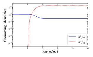
The reheating temperature is given by
| (12) |
Thus, the typical amplitude when perturbative inflaton decay is forbidden can be tuned by choosing the fermion mass and the Yukawa interaction. For a typical value of for detectable GWs, we see from (12) that the reheating temperature will respect the BBN bound Kawasaki:1999na ; Kawasaki:2000en ; Steigman:2007xt . With an understanding of how to reheat the universe, keeping a stable inflaton relic, we will describe the details of our numerical simulation in the following section.
VI Numerical Analysis
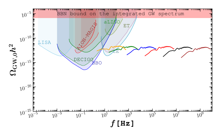
We performed our simulations with lattice points. We kept the dimensionless resonance parameter fixed at for all the simulations. Where the initial values of inflaton oscillation are taken to be . We show the produced GWs spectra in Fig (2). As mentioned earlier, we are interested in the scenarios where the CMB observables do not constrain the quadratic potential during preheating; consequently, we choose the inflaton mass as a free parameter. We have taken its value for each run as . With these values, the ratio of the average energy density of the oscillation modes to the number density of photons defined in (6), are found to be . Now to satisfy the measured value of the current dark matter per photon , we require the value of coupling to have values .
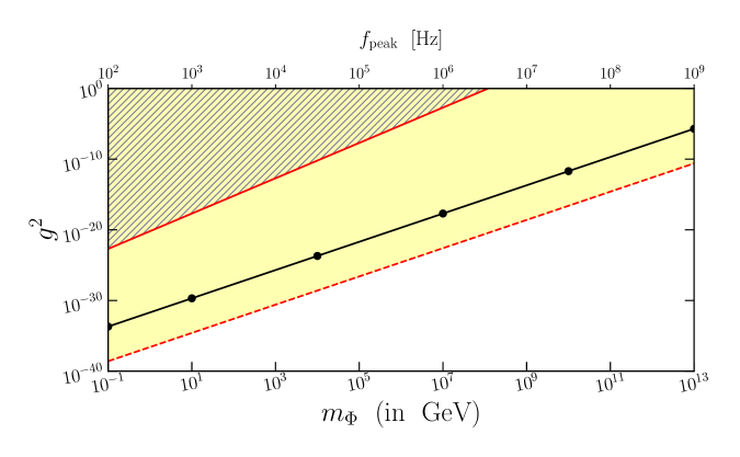
We have plotted the results in (3). The solid red line in the - parameter space satisfies the observed dark matter to photon ratio. Notice that for the cases considered here, when we have inflaton mass below or GeV, the couplings are well within the perturbation limit. However, we have restricted our simulations for those values of , providing us with sufficient resonance without any numerical instabilities. Simulations for all values along the red line in Fig.(3) will result in a large resonance parameter, rendering the lattice simulation afflicted by numerical instabilities. Nevertheless, provided we have sufficient resonance; the amplitude of the GW spectrum only depends on the strength of the resonance parameter while the frequency range depends on the initial energy scale. Consequently, for the same initial energy, changing the coupling will produce a ‘tower’ of GW spectrum within the same frequency range Hyde:2015gwa ; Cai:2021gju ; Figueroa:2022iho . Thus, we can say that those values of the coupling along the red line larger than the simulations performed here will also ensure parametric resonance. Consequently, the corresponding GW signals should also be detectable with various detectors (see Fig. 2). This implies that the coherently oscillating scalar field during (p)-reheating that behaves as type can source a promising candidate for the dark matter. Additionally, we would like to comment that if we consider the production of GWs from coherent scalar while relaxing the scalar field as inflaton, we can have detectable GW signals across a much wider range of frequency bands Cui:2023fbg . For instance, fitting the peak frequency of the red-shifted GWs signal with the energy scale and hence the effective mass, we find the following relation:
| (13) |
Hence, depending on the scalar field mass, we can move to the low-frequency GWs detector bands. All these scenarios could be interesting to explore in light of recently detected GWs background by the North American Nanohertz Observatory for Gravitational Waves (NANOGrav) NANOGrav:2023gor . A comprehensive analysis of the amplitude of GW spectrum involving various interactions between the inflaton and the Higgs field, along with the effects of various initial conditions and a broad range of parameters of interest, will be examined in a future publication (also see Refs. Hyde:2015gwa ; Sang:2019ndv ; Cai:2021gju ; Ashoorioon:2022raz ; Figueroa:2022iho for similar works along this direction).
VII Discussion and Conclusion
In a nutshell, we studied the inflaton behaving as the dark matter of the Universe. We summarize our main findings below:
-
•
We showed in a (p)-reheating scenario, the inflaton starts to oscillate, and its zeroth mode energy remnant behaves as nonthermal dark matter as our observable current Universe satisfying the relic density (cf. Eq. 6). We investigated the impact of resonance parameters on dark matter production via lattice simulation in the oscillating regimes for such an oscillating scenario.
-
•
In such a nonthermal origin of dark matter without any interaction with the visible or the SM sector, it is impossible to have laboratory tests for the DM candidate. We showed that the generated gravitational waves could be a viable detection channel during such an oscillatory period with its typical spectrum, as shown in Fig 2.
-
•
In Fig 3, we showed the allowed parameter space of the coupling and the effective mass of the coherent oscillating inflaton , which satisfy the observed DM mass to photon ratio. If we have sufficient resonance, the amplitude of the produced GWs is independent of the energy scale of the inflation (cf Fig (2)). Thus, we found that for GeV, the generated stochastic signals of GWs will be of sufficient amplitude to be detectable in various planned and proposed detectors while also explaining the origin of dark matter as the remnant inflaton component.
-
•
As depicted in Fig 2, for the higher mass range (GeV), the coupling required to satisfy the observed dark matter relic is excluded by perturbative limit. Moreover, the allowed coupling range will overproduce dark matter and, hence, not allowed when considering inflaton as dark matter. For the lower end, although the couplings required to satisfy the dark matter relic are within the perturbative limit, the resulting resonance parameters became so large that the simulations became numerically unstable. However, in principle, the GWs produced in such parameter regions should also be detectable. Thus, the lower-mass ranges GeV provide an interesting parameter space for the DM probe using GWs detectors.
-
•
We can probe mass scales ( TeV) otherwise not accessible to colliders or any other laboratory physics. There is huge interest in the community to find the detection principles of high-frequency gravitational gaves Aggarwal:2020olq ; Berlin:2021txa ; Domcke:2022rgu . With more advanced detectors, although we may be able to probe high-scale inflationary scenarios, the paradigm of inflation as the dark matter may be in tension within the scope of simple four-legged interaction as considered here.
We have thus explored a novel alternative to the thermal WIMP dark matter scenario in context to the non-thermal production of dark matter in the early Universe. The inflaton itself starts to behave as dark matter in late times, with the energy density stored during the oscillations of the (p)-reheating era. Due to no other or negligible interactions being present between the inflaton sector (dark sector) and the visible sector, we showed our prospects of detecting such non-thermal dark matter candidates within the measurements of SBGW in current and future GW detectors. We envisage our results will be the commencement of huge activity in this direction, whereas an alternative to hunt for various non-thermal dark matter production mechanisms which are otherwise not traceable in laboratory-based or astrophysical searches and, therefore, not in traditional DM detectors due to very feeble or no coupling between the visible and the dark sectors but in GW detectors in the near future, particularly when LIGO has already put bounds 2009Natur.460..990A , and LIGO-VIRGO has further searched for such SGWB KAGRA:2021mth from primordial sources as described in Romero:2021kby .
Acknowledgments
Authors thank Rouzbeh Allahverdi, Nicolas Bernal, Lucien Hertier, Tomasz Krajewski, Marek Lewicki, Anupam Mazumdar, Kyohei Mukaida, Myeonghun Park, and Yuko Urakawa for helpful comments. The study of P. S. is financially supported by the Seoul National University of Science and Technology. The simulations are performed in Dark cluster at Seoultech.
Appendix A Towards Inflationary model building for reheating with detectable GWs signal
The effective mass in most canonical inflationary models is constrained by the amplitude of the scalar spectrum at the CMB scales. For instance, in the simple one-parameter chaotic potential, the value of the mass is fixed at . Looking beyond, the extra parameter models may provide us with some freedom. The currently observationally favored alpha-attractor models, for instance, the super gravity-inspired T-models having the inflationary potential reduces to around the minima. Hence, the effective mass can be written as , where is the amplitude of the potential’s plateau and is a free mass scale describing the width of the potential. In this case, however, it turns out that the observed amplitude of the scalar perturbations imposes approximately , so we have for all values of Antusch:2021aiw . Consequently, the effective mass is the same as the vanilla chaotic inflation 444We thank the referee for pointing this out to us.. Thus, we must expand our search for suitable models in other directions. We list below some models where we can take the effective mass during preheating as a free parameter and describe the associated challenges.
A.1 Two-field hybrid inflation
To make the effective mass a free parameter, the authors in Easther:2006vd assumed that the full potential during inflation is given by:
| (14) |
During inflation, when , stays in its false . Thus, the effective potential during inflation is
| (15) |
The auxiliary field becomes tachyonic when and evolves towards its true vacuum at . Assuming , the potential reduces to
| (16) |
Now, in the limit , The effective potential is given by
| (17) |
where , and, consequently, the effective mass for the inflaton can be taken as a free parameter. However, if and during inflation when , the potential in (16) will result in blue tilted scalar spectra (). Although such blue-tilted spectra have implications for resolving the Hubble tension Takahashi:2021bti ; Jiang:2022uyg ; Ye:2022efx , such spectra are ruled out from observations.
A.2 A model in the framework of -attractor
A broad class of inflationary models defined in terms of a parameter in the context of supergravity are the well-known -attractors. The aforementioned parameter determines the curvature and cutoff of these models. These models are known to predict some universal results of the inflationary observables, viz., the spectral index () and the tensor-to-scalar ratio (). There are several inequivalent formalisms to introduce the cosmological -attractors which eventually leads to the following Einstein frame Lagrangian Kallosh:2014rga :
| (18) |
which after rescaling of the field
| (19) |
Finally, using the scalar field redefinition , we arrive at the following form of Lagrangian in the Einstein frame with a canonically normalized kinetic term:
| (20) |
| (21) |
which will have step-like transitions. We will only concentrate on the case for the rest of our analysis.
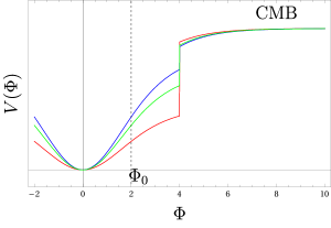
We take that determines the normalization of the potential in the flat region to for matching the predictions of the model with the CMB observables. determines the appearance of the step. The inflationary potential is found to be:
| (22) |
We have expressed all the dimensionful quantities in the units of and . In practice, we can use continuous step function, for instance, for numerical stability when solving the equations for the background inflationary dynamics and perturbations. The effective mass around the minima:
| (23) |
Now, being derivatives of the -attractor models, these models with steps can easily produce the necessary CMB observables. For instance, taking and we can have and while the amplitude of power spectrum fixes the value of to be . This will make the effective mass around the minima . Increasing will decrease the but will require tuning the other parameters. In all cases, the only requirement for the preheating scenario to work is that the position of the step is at higher field values compared to the initial amplitude of the inflaton for simulation (). In the above case, we have taken and . Such models can also boost the scalar power spectrum, which has interesting applications for Primordial black holes and secondary gravitational waves Kefala:2020xsx ; Dalianis:2021iig . It is important to mention that to make as low as in the MeV range for the above model, we will need to take an extremely large height of the step. This may result in a kination phase after the end of inflation that can make the relation between the effective mass of inflaton and the observed GWs signal more convoluted.
At this point, we must emphasize that the models listed above are only suggestive ways of making the effective mass a free parameter and looking for a more realistic model is still an open issue. We adjourn the details of model building and parameter explorations for future work.
References
- (1) G. Jungman, M. Kamionkowski, and K. Griest, “Supersymmetric dark matter,” Phys. Rept. 267 (1996) 195–373, arXiv:hep-ph/9506380.
- (2) G. Bertone, D. Hooper, and J. Silk, “Particle dark matter: Evidence, candidates and constraints,” Phys. Rept. 405 (2005) 279–390, arXiv:hep-ph/0404175.
- (3) J. L. Feng, “Dark Matter Candidates from Particle Physics and Methods of Detection,” Ann. Rev. Astron. Astrophys. 48 (2010) 495–545, arXiv:1003.0904 [astro-ph.CO].
- (4) B. W. Lee and S. Weinberg, “Cosmological Lower Bound on Heavy Neutrino Masses,” Phys. Rev. Lett. 39 (1977) 165–168.
- (5) R. J. Scherrer and M. S. Turner, “On the Relic, Cosmic Abundance of Stable Weakly Interacting Massive Particles,” Phys. Rev. D 33 (1986) 1585. [Erratum: Phys.Rev.D 34, 3263 (1986)].
- (6) M. Srednicki, R. Watkins, and K. A. Olive, “Calculations of Relic Densities in the Early Universe,” Nucl. Phys. B 310 (1988) 693.
- (7) P. Gondolo and G. Gelmini, “Cosmic abundances of stable particles: Improved analysis,” Nucl. Phys. B 360 (1991) 145–179.
- (8) PandaX-II Collaboration, X. Cui et al., “Dark Matter Results From 54-Ton-Day Exposure of PandaX-II Experiment,” Phys. Rev. Lett. 119 no. 18, (2017) 181302, arXiv:1708.06917 [astro-ph.CO].
- (9) PandaX Collaboration, H. Zhang et al., “Dark matter direct search sensitivity of the PandaX-4T experiment,” Sci. China Phys. Mech. Astron. 62 no. 3, (2019) 31011, arXiv:1806.02229 [physics.ins-det].
- (10) XENON Collaboration, E. Aprile et al., “Projected WIMP sensitivity of the XENONnT dark matter experiment,” JCAP 11 (2020) 031, arXiv:2007.08796 [physics.ins-det].
- (11) XENON Collaboration, E. Aprile et al., “Dark Matter Search Results from a One Ton-Year Exposure of XENON1T,” Phys. Rev. Lett. 121 no. 11, (2018) 111302, arXiv:1805.12562 [astro-ph.CO].
- (12) LZ Collaboration, D. S. Akerib et al., “Projected WIMP sensitivity of the LUX-ZEPLIN dark matter experiment,” Phys. Rev. D 101 no. 5, (2020) 052002, arXiv:1802.06039 [astro-ph.IM].
- (13) DARWIN Collaboration, J. Aalbers et al., “DARWIN: towards the ultimate dark matter detector,” JCAP 11 (2016) 017, arXiv:1606.07001 [astro-ph.IM].
- (14) H.E.S.S. Collaboration, H. Abdallah et al., “Search for dark matter annihilations towards the inner Galactic halo from 10 years of observations with H.E.S.S,” Phys. Rev. Lett. 117 no. 11, (2016) 111301, arXiv:1607.08142 [astro-ph.HE].
- (15) MAGIC, Fermi-LAT Collaboration, M. L. Ahnen et al., “Limits to Dark Matter Annihilation Cross-Section from a Combined Analysis of MAGIC and Fermi-LAT Observations of Dwarf Satellite Galaxies,” JCAP 02 (2016) 039, arXiv:1601.06590 [astro-ph.HE].
- (16) ATLAS Collaboration, M. Aaboud et al., “Search for dark matter and other new phenomena in events with an energetic jet and large missing transverse momentum using the ATLAS detector,” JHEP 01 (2018) 126, arXiv:1711.03301 [hep-ex].
- (17) CMS Collaboration, A. M. Sirunyan et al., “Search for new physics in final states with an energetic jet or a hadronically decaying or boson and transverse momentum imbalance at ,” Phys. Rev. D 97 no. 9, (2018) 092005, arXiv:1712.02345 [hep-ex].
- (18) J. McDonald, “Thermally generated gauge singlet scalars as selfinteracting dark matter,” Phys. Rev. Lett. 88 (2002) 091304, arXiv:hep-ph/0106249.
- (19) L. J. Hall, K. Jedamzik, J. March-Russell, and S. M. West, “Freeze-In Production of FIMP Dark Matter,” JHEP 03 (2010) 080, arXiv:0911.1120 [hep-ph].
- (20) N. Bernal, M. Heikinheimo, T. Tenkanen, K. Tuominen, and V. Vaskonen, “The Dawn of FIMP Dark Matter: A Review of Models and Constraints,” Int. J. Mod. Phys. A 32 no. 27, (2017) 1730023, arXiv:1706.07442 [hep-ph].
- (21) T. Moroi, M. Yamaguchi, and T. Yanagida, “On the solution to the Polonyi problem with 0 (10-TeV) gravitino mass in supergravity,” Phys. Lett. B 342 (1995) 105–110, arXiv:hep-ph/9409367.
- (22) M. Kawasaki, T. Moroi, and T. Yanagida, “Constraint on the reheating temperature from the decay of the Polonyi field,” Phys. Lett. B 370 (1996) 52–58, arXiv:hep-ph/9509399.
- (23) T. Moroi and L. Randall, “Wino cold dark matter from anomaly mediated SUSY breaking,” Nucl. Phys. B 570 (2000) 455–472, arXiv:hep-ph/9906527.
- (24) K. S. Jeong, M. Shimosuka, and M. Yamaguchi, “Light Higgsino in Heavy Gravitino Scenario with Successful Electroweak Symmetry Breaking,” JHEP 09 (2012) 050, arXiv:1112.5293 [hep-ph].
- (25) J. Ellis, M. A. G. Garcia, D. V. Nanopoulos, K. A. Olive, and M. Peloso, “Post-Inflationary Gravitino Production Revisited,” JCAP 03 (2016) 008, arXiv:1512.05701 [astro-ph.CO].
- (26) K. Harigaya, M. Kawasaki, K. Mukaida, and M. Yamada, “Dark Matter Production in Late Time Reheating,” Phys. Rev. D 89 no. 8, (2014) 083532, arXiv:1402.2846 [hep-ph].
- (27) M. A. G. Garcia and M. A. Amin, “Prethermalization production of dark matter,” Phys. Rev. D 98 no. 10, (2018) 103504, arXiv:1806.01865 [hep-ph].
- (28) K. Harigaya, K. Mukaida, and M. Yamada, “Dark Matter Production during the Thermalization Era,” JHEP 07 (2019) 059, arXiv:1901.11027 [hep-ph].
- (29) M. A. G. Garcia, K. Kaneta, Y. Mambrini, and K. A. Olive, “Reheating and Post-inflationary Production of Dark Matter,” Phys. Rev. D 101 no. 12, (2020) 123507, arXiv:2004.08404 [hep-ph].
- (30) D. J. H. Chung, E. W. Kolb, and A. Riotto, “Superheavy dark matter,” Phys. Rev. D 59 (1998) 023501, arXiv:hep-ph/9802238.
- (31) D. J. H. Chung, E. W. Kolb, and A. Riotto, “Nonthermal supermassive dark matter,” Phys. Rev. Lett. 81 (1998) 4048–4051, arXiv:hep-ph/9805473.
- (32) R. T. Co, L. J. Hall, and K. Harigaya, “QCD Axion Dark Matter with a Small Decay Constant,” Phys. Rev. Lett. 120 no. 21, (2018) 211602, arXiv:1711.10486 [hep-ph].
- (33) R. Brout, F. Englert, and E. Gunzig, “The Creation of the Universe as a Quantum Phenomenon,” Annals Phys. 115 (1978) 78.
- (34) K. Sato, “First Order Phase Transition of a Vacuum and Expansion of the Universe,” Mon. Not. Roy. Astron. Soc. 195 (1981) 467–479.
- (35) A. H. Guth, “The Inflationary Universe: A Possible Solution to the Horizon and Flatness Problems,” Phys. Rev. D 23 (1981) 347–356.
- (36) A. D. Linde, “A New Inflationary Universe Scenario: A Possible Solution of the Horizon, Flatness, Homogeneity, Isotropy and Primordial Monopole Problems,” Phys. Lett. B 108 (1982) 389–393.
- (37) A. A. Starobinsky, “Dynamics of Phase Transition in the New Inflationary Universe Scenario and Generation of Perturbations,” Phys. Lett. B 117 (1982) 175–178.
- (38) A. R. Liddle and L. A. Urena-Lopez, “Inflation, dark matter and dark energy in the string landscape,” Phys. Rev. Lett. 97 (2006) 161301, arXiv:astro-ph/0605205.
- (39) V. H. Cardenas, “Inflation, Reheating and Dark Matter,” Phys. Rev. D 75 (2007) 083512, arXiv:astro-ph/0701624.
- (40) G. Panotopoulos, “A Brief note on how to unify dark matter, dark energy, and inflation,” Phys. Rev. D 75 (2007) 127301, arXiv:0706.2237 [hep-ph].
- (41) A. R. Liddle, C. Pahud, and L. A. Urena-Lopez, “Triple unification of inflation, dark matter, and dark energy using a single field,” Phys. Rev. D 77 (2008) 121301, arXiv:0804.0869 [astro-ph].
- (42) N. Bose and A. S. Majumdar, “Unified Model of -Inflation, Dark Matter & Dark Energy,” Phys. Rev. D 80 (2009) 103508, arXiv:0907.2330 [astro-ph.CO].
- (43) R. N. Lerner and J. McDonald, “Gauge singlet scalar as inflaton and thermal relic dark matter,” Phys. Rev. D 80 (2009) 123507, arXiv:0909.0520 [hep-ph].
- (44) J. De-Santiago and J. L. Cervantes-Cota, “Generalizing a Unified Model of Dark Matter, Dark Energy, and Inflation with Non Canonical Kinetic Term,” Phys. Rev. D 83 (2011) 063502, arXiv:1102.1777 [astro-ph.CO].
- (45) V. V. Khoze, “Inflation and Dark Matter in the Higgs Portal of Classically Scale Invariant Standard Model,” JHEP 11 (2013) 215, arXiv:1308.6338 [hep-ph].
- (46) K. Mukaida and K. Nakayama, “Dark Matter Chaotic Inflation in Light of BICEP2,” JCAP 08 (2014) 062, arXiv:1404.1880 [hep-ph].
- (47) M. Fairbairn, R. Hogan, and D. J. E. Marsh, “Unifying inflation and dark matter with the Peccei-Quinn field: observable axions and observable tensors,” Phys. Rev. D 91 no. 2, (2015) 023509, arXiv:1410.1752 [hep-ph].
- (48) M. Bastero-Gil, R. Cerezo, and J. G. Rosa, “Inflaton dark matter from incomplete decay,” Phys. Rev. D 93 no. 10, (2016) 103531, arXiv:1501.05539 [hep-ph].
- (49) F. Kahlhoefer and J. McDonald, “WIMP Dark Matter and Unitarity-Conserving Inflation via a Gauge Singlet Scalar,” JCAP 11 (2015) 015, arXiv:1507.03600 [astro-ph.CO].
- (50) T. Tenkanen, “Feebly Interacting Dark Matter Particle as the Inflaton,” JHEP 09 (2016) 049, arXiv:1607.01379 [hep-ph].
- (51) R. Daido, F. Takahashi, and W. Yin, “The ALP miracle: unified inflaton and dark matter,” JCAP 05 (2017) 044, arXiv:1702.03284 [hep-ph].
- (52) S. Choubey and A. Kumar, “Inflation and Dark Matter in the Inert Doublet Model,” JHEP 11 (2017) 080, arXiv:1707.06587 [hep-ph].
- (53) R. Daido, F. Takahashi, and W. Yin, “The ALP miracle revisited,” JHEP 02 (2018) 104, arXiv:1710.11107 [hep-ph].
- (54) D. Hooper, G. Krnjaic, A. J. Long, and S. D. Mcdermott, “Can the Inflaton Also Be a Weakly Interacting Massive Particle?,” Phys. Rev. Lett. 122 no. 9, (2019) 091802, arXiv:1807.03308 [hep-ph].
- (55) D. Borah, P. S. B. Dev, and A. Kumar, “TeV scale leptogenesis, inflaton dark matter and neutrino mass in a scotogenic model,” Phys. Rev. D 99 no. 5, (2019) 055012, arXiv:1810.03645 [hep-ph].
- (56) A. Torres Manso and J. a. G. Rosa, “-inflaton dark matter,” JHEP 02 (2019) 020, arXiv:1811.02302 [hep-ph].
- (57) J. a. G. Rosa and L. B. Ventura, “Warm Little Inflaton becomes Cold Dark Matter,” Phys. Rev. Lett. 122 no. 16, (2019) 161301, arXiv:1811.05493 [hep-ph].
- (58) J. P. B. Almeida, N. Bernal, J. Rubio, and T. Tenkanen, “Hidden inflation dark matter,” JCAP 03 (2019) 012, arXiv:1811.09640 [hep-ph].
- (59) Planck Collaboration, N. Aghanim et al., “Planck 2018 results. VI. Cosmological parameters,” Astron. Astrophys. 641 (2020) A6, arXiv:1807.06209 [astro-ph.CO]. [Erratum: Astron.Astrophys. 652, C4 (2021)].
- (60) A. Paul, A. Ghoshal, A. Chatterjee, and S. Pal, “Inflation, (P)reheating and Neutrino Anomalies: Production of Sterile Neutrinos with Secret Interactions,” Eur. Phys. J. C 79 no. 10, (2019) 818, arXiv:1808.09706 [astro-ph.CO].
- (61) L. Kofman, A. D. Linde, and A. A. Starobinsky, “Reheating after inflation,” Phys. Rev. Lett. 73 (1994) 3195–3198, arXiv:hep-th/9405187.
- (62) L. Kofman, A. D. Linde, and A. A. Starobinsky, “Towards the theory of reheating after inflation,” Phys. Rev. D 56 (1997) 3258–3295, arXiv:hep-ph/9704452.
- (63) K. Mukaida, K. Nakayama, and M. Takimoto, “Fate of Symmetric Scalar Field,” JHEP 12 (2013) 053, arXiv:1308.4394 [hep-ph].
- (64) S. Y. Khlebnikov and I. I. Tkachev, “Relic gravitational waves produced after preheating,” Phys. Rev. D 56 (1997) 653–660, arXiv:hep-ph/9701423.
- (65) R. Easther and E. A. Lim, “Stochastic gravitational wave production after inflation,” JCAP 04 (2006) 010, arXiv:astro-ph/0601617.
- (66) R. Easther, J. T. Giblin, Jr., and E. A. Lim, “Gravitational Wave Production At The End Of Inflation,” Phys. Rev. Lett. 99 (2007) 221301, arXiv:astro-ph/0612294.
- (67) R. Easther, J. T. Giblin, and E. A. Lim, “Gravitational Waves From the End of Inflation: Computational Strategies,” Phys. Rev. D 77 (2008) 103519, arXiv:0712.2991 [astro-ph].
- (68) J. F. Dufaux, A. Bergman, G. N. Felder, L. Kofman, and J.-P. Uzan, “Theory and Numerics of Gravitational Waves from Preheating after Inflation,” Phys. Rev. D 76 (2007) 123517, arXiv:0707.0875 [astro-ph].
- (69) J. Garcia-Bellido and D. G. Figueroa, “A stochastic background of gravitational waves from hybrid preheating,” Phys. Rev. Lett. 98 (2007) 061302, arXiv:astro-ph/0701014.
- (70) J. Garcia-Bellido, D. G. Figueroa, and A. Sastre, “A Gravitational Wave Background from Reheating after Hybrid Inflation,” Phys. Rev. D 77 (2008) 043517, arXiv:0707.0839 [hep-ph].
- (71) J.-F. Dufaux, G. Felder, L. Kofman, and O. Navros, “Gravity Waves from Tachyonic Preheating after Hybrid Inflation,” JCAP 03 (2009) 001, arXiv:0812.2917 [astro-ph].
- (72) A. Ringwald and C. Tamarit, “Revealing the cosmic history with gravitational waves,” Phys. Rev. D 106 no. 6, (2022) 063027, arXiv:2203.00621 [hep-ph].
- (73) J.-F. Dufaux, D. G. Figueroa, and J. Garcia-Bellido, “Gravitational Waves from Abelian Gauge Fields and Cosmic Strings at Preheating,” Phys. Rev. D 82 (2010) 083518, arXiv:1006.0217 [astro-ph.CO].
- (74) P. Adshead, J. T. Giblin, and Z. J. Weiner, “Gravitational waves from gauge preheating,” Phys. Rev. D 98 no. 4, (2018) 043525, arXiv:1805.04550 [astro-ph.CO].
- (75) P. Adshead, J. T. Giblin, M. Pieroni, and Z. J. Weiner, “Constraining axion inflation with gravitational waves from preheating,” Phys. Rev. D 101 no. 8, (2020) 083534, arXiv:1909.12842 [astro-ph.CO].
- (76) S. Antusch, F. Cefala, and S. Orani, “Gravitational waves from oscillons after inflation,” Phys. Rev. Lett. 118 no. 1, (2017) 011303, arXiv:1607.01314 [astro-ph.CO]. [Erratum: Phys.Rev.Lett. 120, 219901 (2018)].
- (77) M. A. Amin, J. Braden, E. J. Copeland, J. T. Giblin, C. Solorio, Z. J. Weiner, and S.-Y. Zhou, “Gravitational waves from asymmetric oscillon dynamics?,” Phys. Rev. D 98 (2018) 024040, arXiv:1803.08047 [astro-ph.CO].
- (78) K. D. Lozanov and M. A. Amin, “Gravitational perturbations from oscillons and transients after inflation,” Phys. Rev. D 99 no. 12, (2019) 123504, arXiv:1902.06736 [astro-ph.CO].
- (79) J. J. M. Carrasco, R. Kallosh, and A. Linde, “Cosmological Attractors and Initial Conditions for Inflation,” Phys. Rev. D 92 no. 6, (2015) 063519, arXiv:1506.00936 [hep-th].
- (80) R. Kallosh, A. Linde, and D. Roest, “Superconformal Inflationary -Attractors,” JHEP 11 (2013) 198, arXiv:1311.0472 [hep-th].
- (81) A. D. Linde, “Hybrid inflation,” Phys. Rev. D 49 (1994) 748–754, arXiv:astro-ph/9307002.
- (82) D. H. Lyth and A. Riotto, “Particle physics models of inflation and the cosmological density perturbation,” Phys. Rept. 314 (1999) 1–146, arXiv:hep-ph/9807278.
- (83) A. Mazumdar and J. Rocher, “Particle physics models of inflation and curvaton scenarios,” Phys. Rept. 497 (2011) 85–215, arXiv:1001.0993 [hep-ph].
- (84) N. Kitajima, J. Soda, and Y. Urakawa, “Gravitational wave forest from string axiverse,” JCAP 10 (2018) 008, arXiv:1807.07037 [astro-ph.CO].
- (85) G. N. Felder and I. Tkachev, “LATTICEEASY: A Program for lattice simulations of scalar fields in an expanding universe,” Comput. Phys. Commun. 178 (2008) 929–932, arXiv:hep-ph/0011159.
- (86) A. V. Frolov, “DEFROST: A New Code for Simulating Preheating after Inflation,” JCAP 11 (2008) 009, arXiv:0809.4904 [hep-ph].
- (87) R. Easther, H. Finkel, and N. Roth, “PSpectRe: A Pseudo-Spectral Code for (P)reheating,” JCAP 10 (2010) 025, arXiv:1005.1921 [astro-ph.CO].
- (88) Z. Huang, “The Art of Lattice and Gravity Waves from Preheating,” Phys. Rev. D 83 (2011) 123509, arXiv:1102.0227 [astro-ph.CO].
- (89) D. G. Figueroa, A. Florio, F. Torrenti, and W. Valkenburg, “CosmoLattice: A modern code for lattice simulations of scalar and gauge field dynamics in an expanding universe,” Comput. Phys. Commun. 283 (2023) 108586, arXiv:2102.01031 [astro-ph.CO].
- (90) S.-Y. Zhou, E. J. Copeland, R. Easther, H. Finkel, Z.-G. Mou, and P. M. Saffin, “Gravitational Waves from Oscillon Preheating,” JHEP 10 (2013) 026, arXiv:1304.6094 [astro-ph.CO].
- (91) D. I. Podolsky, G. N. Felder, L. Kofman, and M. Peloso, “Equation of state and beginning of thermalization after preheating,” Phys. Rev. D 73 (2006) 023501, arXiv:hep-ph/0507096.
- (92) D. Maity and P. Saha, “(P)reheating after minimal Plateau Inflation and constraints from CMB,” JCAP 07 (2019) 018, arXiv:1811.11173 [astro-ph.CO].
- (93) P. Saha, S. Anand, and L. Sriramkumar, “Accounting for the time evolution of the equation of state parameter during reheating,” Phys. Rev. D 102 no. 10, (2020) 103511, arXiv:2005.01874 [astro-ph.CO].
- (94) S. Antusch, D. G. Figueroa, K. Marschall, and F. Torrenti, “Energy distribution and equation of state of the early Universe: matching the end of inflation and the onset of radiation domination,” Phys. Lett. B 811 (2020) 135888, arXiv:2005.07563 [astro-ph.CO].
- (95) N. Okada and Q. Shafi, “WIMP Dark Matter Inflation with Observable Gravity Waves,” Phys. Rev. D 84 (2011) 043533, arXiv:1007.1672 [hep-ph].
- (96) J. F. Dufaux, G. N. Felder, L. Kofman, M. Peloso, and D. Podolsky, “Preheating with trilinear interactions: Tachyonic resonance,” JCAP 07 (2006) 006, arXiv:hep-ph/0602144.
- (97) E. W. Kolb, A. Notari, and A. Riotto, “On the reheating stage after inflation,” Phys. Rev. D 68 (2003) 123505, arXiv:hep-ph/0307241.
- (98) M. Kawasaki, K. Kohri, and N. Sugiyama, “Cosmological constraints on late time entropy production,” Phys. Rev. Lett. 82 (1999) 4168, arXiv:astro-ph/9811437.
- (99) M. Kawasaki, K. Kohri, and N. Sugiyama, “MeV scale reheating temperature and thermalization of neutrino background,” Phys. Rev. D 62 (2000) 023506, arXiv:astro-ph/0002127.
- (100) G. Steigman, “Primordial Nucleosynthesis in the Precision Cosmology Era,” Ann. Rev. Nucl. Part. Sci. 57 (2007) 463–491, arXiv:0712.1100 [astro-ph].
- (101) J. M. Hyde, “Sensitivity of gravitational waves from preheating to a scalar field’s interactions,” Phys. Rev. D 92 no. 4, (2015) 044026, arXiv:1502.07660 [hep-ph].
- (102) R.-G. Cai, Z.-K. Guo, P.-Z. Ding, C.-J. Fu, and J. Liu, “Dependence of the amplitude of gravitational waves from preheating on the inflationary energy scale,” Phys. Rev. D 105 no. 2, (2022) 023507, arXiv:2105.00427 [astro-ph.CO].
- (103) D. G. Figueroa, A. Florio, N. Loayza, and M. Pieroni, “Spectroscopy of particle couplings with gravitational waves,” Phys. Rev. D 106 no. 6, (2022) 063522, arXiv:2202.05805 [astro-ph.CO].
- (104) Y. Cui, P. Saha, and E. I. Sfakianakis, “Gravitational Wave Symphony from Oscillating Spectator Scalar Fields,” arXiv:2310.13060 [hep-ph].
- (105) NANOGrav Collaboration, G. Agazie et al., “The NANOGrav 15 yr Data Set: Evidence for a Gravitational-wave Background,” Astrophys. J. Lett. 951 no. 1, (2023) L8, arXiv:2306.16213 [astro-ph.HE].
- (106) Y. Sang and Q.-G. Huang, “Stochastic Gravitational-Wave Background from Axion-Monodromy Oscillons in String Theory During Preheating,” Phys. Rev. D 100 no. 6, (2019) 063516, arXiv:1905.00371 [astro-ph.CO].
- (107) A. Ashoorioon, K. Rezazadeh, and A. Rostami, “NANOGrav signal from the end of inflation and the LIGO mass and heavier primordial black holes,” Phys. Lett. B 835 (2022) 137542, arXiv:2202.01131 [astro-ph.CO].
- (108) N. Aggarwal et al., “Challenges and opportunities of gravitational-wave searches at MHz to GHz frequencies,” Living Rev. Rel. 24 no. 1, (2021) 4, arXiv:2011.12414 [gr-qc].
- (109) A. Berlin, D. Blas, R. Tito D’Agnolo, S. A. R. Ellis, R. Harnik, Y. Kahn, and J. Schütte-Engel, “Detecting high-frequency gravitational waves with microwave cavities,” Phys. Rev. D 105 no. 11, (2022) 116011, arXiv:2112.11465 [hep-ph].
- (110) V. Domcke, C. Garcia-Cely, and N. L. Rodd, “Novel Search for High-Frequency Gravitational Waves with Low-Mass Axion Haloscopes,” Phys. Rev. Lett. 129 no. 4, (2022) 041101, arXiv:2202.00695 [hep-ph].
- (111) B. P. Abbott, R. Abbott, F. Acernese, R. Adhikari, P. Ajith, B. Allen, G. Allen, M. Alshourbagy, R. S. Amin, S. B. Anderson, and et al., “An upper limit on the stochastic gravitational-wave background of cosmological origin,” Nature (London) 460 no. 7258, (Aug., 2009) 990–994, arXiv:0910.5772 [astro-ph.CO].
- (112) KAGRA, Virgo, LIGO Scientific Collaboration, R. Abbott et al., “Search for anisotropic gravitational-wave backgrounds using data from Advanced LIGO and Advanced Virgo’s first three observing runs,” Phys. Rev. D 104 no. 2, (2021) 022005, arXiv:2103.08520 [gr-qc].
- (113) A. Romero, K. Martinovic, T. A. Callister, H.-K. Guo, M. Martínez, M. Sakellariadou, F.-W. Yang, and Y. Zhao, “Implications for First-Order Cosmological Phase Transitions from the Third LIGO-Virgo Observing Run,” Phys. Rev. Lett. 126 no. 15, (2021) 151301, arXiv:2102.01714 [hep-ph].
- (114) S. Antusch, D. G. Figueroa, K. Marschall, and F. Torrenti, “Characterizing the postinflationary reheating history: Single daughter field with quadratic-quadratic interaction,” Phys. Rev. D 105 no. 4, (2022) 043532, arXiv:2112.11280 [astro-ph.CO].
- (115) F. Takahashi and W. Yin, “Cosmological implications of in light of the Hubble tension,” Phys. Lett. B 830 (2022) 137143, arXiv:2112.06710 [astro-ph.CO].
- (116) J.-Q. Jiang and Y.-S. Piao, “Toward early dark energy and ns=1 with Planck, ACT, and SPT observations,” Phys. Rev. D 105 no. 10, (2022) 103514, arXiv:2202.13379 [astro-ph.CO].
- (117) G. Ye, J.-Q. Jiang, and Y.-S. Piao, “Toward inflation with ns=1 in light of the Hubble tension and implications for primordial gravitational waves,” Phys. Rev. D 106 no. 10, (2022) 103528, arXiv:2205.02478 [astro-ph.CO].
- (118) R. Kallosh, A. Linde, and D. Roest, “Large field inflation and double -attractors,” JHEP 08 (2014) 052, arXiv:1405.3646 [hep-th].
- (119) K. Kefala, G. P. Kodaxis, I. D. Stamou, and N. Tetradis, “Features of the inflaton potential and the power spectrum of cosmological perturbations,” Phys. Rev. D 104 no. 2, (2021) 023506, arXiv:2010.12483 [astro-ph.CO].
- (120) I. Dalianis, G. P. Kodaxis, I. D. Stamou, N. Tetradis, and A. Tsigkas-Kouvelis, “Spectrum oscillations from features in the potential of single-field inflation,” Phys. Rev. D 104 no. 10, (2021) 103510, arXiv:2106.02467 [astro-ph.CO].