Mugs: A Multi-Granular Self-Supervised Learning Framework

Abstract

In self-supervised learning, multi-granular features are heavily desired though rarely investigated, as different downstream tasks (e.g., general and fine-grained classification) often require different or multi-granular features, e.g. fine- or coarse-grained one or their mixture. In this work, for the first time, we propose an effective MUlti-Granular Self-supervised learning (Mugs) framework to explicitly learn multi-granular visual features. Mugs has three complementary granular supervisions: 1)​ an instance discrimination supervision (IDS), 2)​ a novel local-group discrimination supervision (LGDS), and 3)​ a group discrimination supervision (GDS). IDS distinguishes different instances to learn instance-level fine-grained features. LGDS aggregates features of an image and its neighbors into a local-group feature, and pulls local-group features from different crops of the same image together and push them away for others. It provides complementary instance supervision to IDS via an extra alignment on local neighbors, and scatters different local-groups separately to increase discriminability. Accordingly, it helps learn high-level fine-grained features at a local-group level. Finally, to prevent similar local-groups from being scattered randomly or far away, GDS brings similar samples close and thus pulls similar local-groups together, capturing coarse-grained features at a (semantic) group level. Consequently, Mugs can capture three granular features that often enjoy higher generality on diverse downstream tasks over single-granular features, e.g. instance-level fine-grained features in contrastive learning. By only pretraining on ImageNet-1K, Mugs sets new SoTA linear probing accuracy 82.1$\%$ on ImageNet-1K and improves previous SoTA by $1.1\%$. It also surpasses SoTAs on other tasks, e.g. transfer learning, detection and segmentation. Codes and models are available at https://github.com/sail-sg/mugs.

1 Introduction

The family of self-supervised learning (SSL) approaches [27, 15, 12, 11, 7, 24, 35] aims to learn highly transferable unsupervised representation for various downstream tasks by training deep models on a large-scale unlabeled dataset. To this end, a pretext task, e.g. jigsaw puzzle [43] or orientation [34], is elaborately designed to generate pseudo labels of unlabeled visual data which are then utilized
to train a model without using manual annotations. Since unlabeled visual data are of huger amount and also much cheaper than the manually annotated data, SSL has been very popularly adopted for visual representation learning recently [27, 11, 7, 24, 62], and is showing greater potential than supervised learning approaches for learning highly-qualified and well-transferable representation.

Motivation. In practice, various downstream tasks in SSL field often require different granular features, such as coarse- or fine-grained features. For instance, general classification downstream tasks distinguish a category from other categories and typically desire coarse-grained features, while fine-grained classification often discriminates subordinate categories and needs more fine-grained features. Actually, many downstream tasks highly desire multi-granular features. Take the classification task on ImageNet-1K [21] as an example. One needs coarse-grained features to distinguish a big category, e.g. dog, from other categories, e.g. bird and car, and also requires fine-grained features to discriminate different subordinate categories, such as Labrador and poodle in the dog category. However, this important multi-granularity requirement is ignored in the current state-of-the-art SSL approaches, including the representative contrastive learning family [26, 27, 32] and clustering learning family [6, 10]. For contrastive learning, its instance discrimination task only aims to distinguish individual instances for learning more instance-level fine-grained features, and does not consider the coarse-grained cluster structure in the data. As a result, it cannot well push semantically similar instances to be close either empirically [62] or theoretically [50], impairing performance, especially for classification downstream tasks. The clustering learning family aims to cluster similar instances into the same cluster and thus learns cluster-level coarse-grained features. In this way, it cannot well handle the downstream tasks that require some fine-grained features. Therefore, in absence of prior feature preference of down stream tasks, one should build an SSL framework to learn multi-granular representation to well handle as many downstream tasks as possible.

Figure 1: ​​Attention visualization on​ “mugs”​ of​ ViT-B​/​16 trained by our Mugs. See more examples in Sec. 4.1.

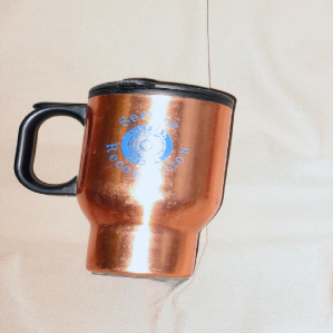
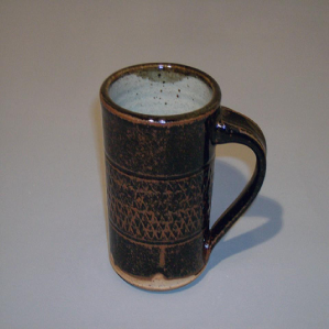
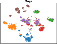
Contributions. In this work, we propose an effective MUlti-Granular Self-supervised learning (Mugs) framework to explicitly learn multi-granular features for visual data. Specifically, Mugs adopts three complementary granular supervisions: 1) instance discrimination supervision (IDS), 2) local-group discrimination supervision (LGDS), and 3) group discrimination supervision (GDS). Inspired by contrastive learning, IDS distinguishes instances via scattering different instance features separately, and thus supervises instance-level fine-grained feature learning. To capture the higher-level fine-grained feature which is also called the “local-group feature” in this work, Mugs proposes a novel and effective LGDS. LGDS aggregates the features of an instance and its few highly similar neighbors into a local-group feature through a small transformer. Then it brings local-group features of different crops from the same image together and pushes them far away for others. This supervision enhances Mugs from two aspects: 1) it provides complementary instance supervision to the above IDS, since it enforces different crops of the same image to have highly similar neighbors, which is an extra challenging alignment, and can boost local-group semantic alignment; 2) it encourages highly-similar instances to constitute small local-groups and scatters these groups separately, boosting more discriminative semantic learning. Finally, GDS is designed to avoid the cases that similar local-groups are scattered randomly or far away. To this end, GDS brings similar samples together and thus pulls similar local-groups close, which captures coarse-grained features at a (semantic) group level. With these complementary supervisions, Mugs can well learn multi-granular data features which can accurately capture the data semantics, e.g. the shapes of “mugs” in ImageNet-1K as illustrated in Fig. 6, and also often enjoy better generality and transferability on diverse downstream tasks than single-granular features.

As shown in Fig. 2 (a), by only pretraining on ImageNet-1K, our Mugs sets a new state-of-the-art (SoTA) 82.1$\%$ linear probing accuracy on ImageNet-1K and surpasses the previous SoTA, i.e. iBOT [61], by a large margin $1.1\%$. Moreover, under different model sizes (see Fig. 2 (a)) and pretraining epochs (see Fig. 2 (b)), Mugs consistently improves previous SoTA pretrained on ImageNet 1K by a non-trivial 0.8% linear probing accuracy. Under other three classification settings, i.e. KNN, fine-tuning the whole network and semi-supervised learning, Mugs also beats previous best methods on the same model. In addition, Mugs shows its advantages on transfer learning, object detection, instance and semantic segmentation tasks. These results well testify the high quality, generality and transferability of the learnt features by Mugs. Note that in this work, we evaluate the effectiveness of Mugs through vision transformer (ViT) [23, 39], as ViT often achieves better performance than CNN of the same model size [49, 39] and also shows great potential to unify vision and language models [28, 2].

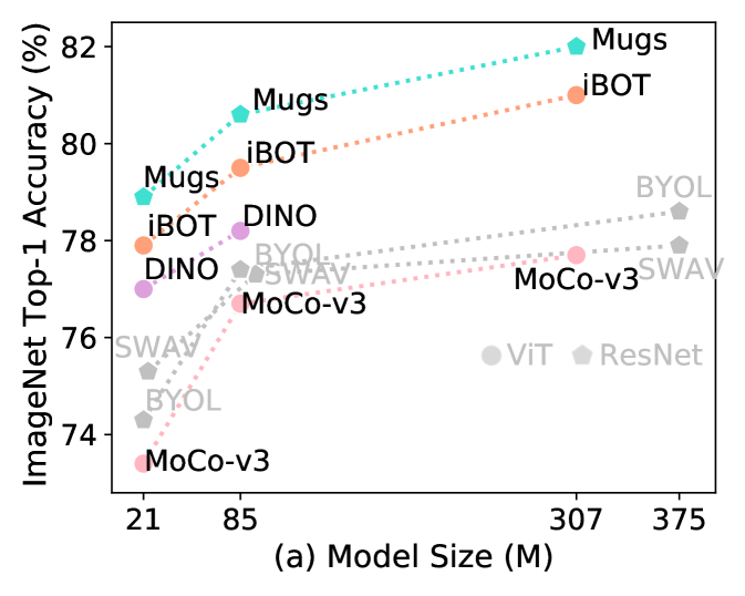
	ViT-S/16	ViT-B/16	ViT-L/16
iBOT	77.9%	79.5%	81.0%
Mugs	78.9%	80.6%	82.1%

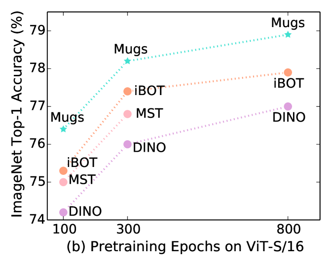
epochs	100	300	800
iBOT	75.3%	77.4%	77.9%
Mugs	76.4%	78.2%	78.9%

Figure 2: Comparison of linear probing accuracy on ImageNet-1K. By pretraining on ImageNet-1K, under different model sizes (see (a)) and pretraining epochs (see (b)), Mugs consistently improves previous SoTA (iBOT) by at least 0.8%.

2 Related works

As an effective family of SSL, contrastive learning [15, 26, 32, 44, 1], e.g., MoCo [27]
and SimCLR [11], has gained much attention recently. Its key is an instance discrimination task which aims to train a network so that the positive pair, i.e. crops of the same image, are close but far from the negatives, namely the crops of other images. Later, BYOL [25] trains a network by only bringing two positives close in the feature space without using any negatives. Though successful, these methods only distinguish individual instances to learn fine-grained feature, and often cannot well push semantically similar instances close, impairing their performance.

Another line of SSL is clustering learning [59, 4, 54, 6, 52, 33, 57, 37], which
assigns pseudo cluster labels for each sample and then trains a network to learn unsupervised representation. For instance, deepcluster [8] uses k-means to cluster all data features and generates pseudo clustering labels which are then used to train a network. PCL [35] and SwAV [7] integrate scalable online clustering approach with contrastive learning via learning cluster prototypes as the positive and negative instances for queries, and achieve promising performance. Recently, DINO [10] and MST [36] propose a much simple online labeling framework that generates pseudo-labels via a momentum teacher. Unfortunately, this clustering family often learns cluster-level coarse-grained (semantic) features, and cannot well handle the downstream tasks which desire fine-grained features.

Finally, the recently proposed masked auto-encoder (MAE) [29, 56, 22, 20, 2] is a new SSL family. It builds on a reconstruction task that randomly masks image patches and then reconstructs the missing pixels or semantic features via an auto-encoder. However, it emphasizes local region reconstruction, and lacks semantic discrimination ability. As a result, for adapting to downstream tasks via only fine-tuning a task head at the top of the pretrained backbone, it performs much worse than contrastive and clustering learning [28, 61]. Indeed, to achieve satisfactory performance, this reconstruction family needs to fine-tune the whole pretrained network for learning global semantics which are necessary for many downstream tasks, e.g. classification. But this requires much higher extra training cost, and also results in very different models for different downstream tasks, which destroys model compatibility and increases practical deployment cost.

Figure 3: Overall framework of Mugs. (a) shows the overall framework. For each image, Mugs respectively performs two random augmentations and feeds two crops into backbones of student and teacher. Next, it adopts three granular supervisions/losses: 1) instance discrimination supervision, 2) local-group discrimination supervision, and 3) group discrimination supervision. Teacher is updated via exponential moving average of student. “sg” denotes stop-gradient. (b) shows the pipeline of local-group modules in both student and teacher. This module averages all patch tokens, and then finds top-$k$ neighbors from memory buffer. Next, it uses a transformer to aggregate the average and its $k$ neighbors to obtain a local-group feature (class token) and feeds it into a local-group head.

3 Multi-granular self-supervised learning

Here we first introduce the overall framework of our MUlti-Granular Self-supervised learning (Mugs), and then elaborate on its three granular supervisions. We evaluate the effectiveness of Mugs through ViT [23, 39] and thus will take ViT as an example to introduce Mugs. This is because 1) with similar model size, ViT shows better performance than CNN [49, 39, 28, 58]; 2) ViT shows great potential for unifying the vision and language models [28, 2].

3.1 Overall Framework

Here we first introduce our motivation. As discussed in Sec. 1, different downstream tasks, e.g. general classification and its fine-grained variant, often require different granular features, e.g. coarse- or fine-grained one. More importantly, many real downstream tasks actually highly desire multi-granular feature. For instance, for classification problems, one needs coarse-grained feature to discriminate animals from other big categories, e.g. plants, since one big category often share much coarse-grained features, e.g. legs and head in animals, leaves and multi-branches in plants. Then to distinguish subcategories in each big category, e.g. dogs and wolves, a slightly lower-level coarse-grained (high-level fine-grained) feature is necessary. Finally, to further discriminate different species in each subcategory, e.g. Labrador dog and poodle dog, more fine-grained feature is actually required. Unfortunately, this important requirement for multi-granular features is seldom brought to front and even totally ignored in existing SSL methods.

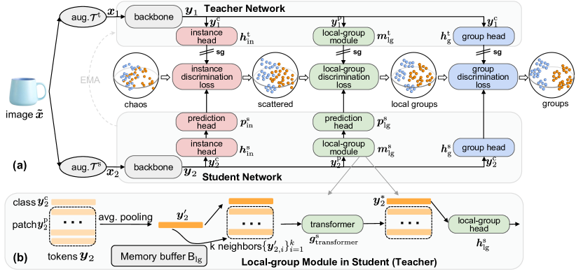
To alleviate this issue, we propose a simple but effective Mugs framework to learn multi-granular features, which can better satisfy different granular feature requirements of various downstream tasks and thus enjoy higher transferability and generality than single-granular features. As illustrated in Fig. 3 (a), given an image $\widetilde{\bm{x}}$, Mugs independently performers augmentations $\footnotesize{\mathcal{T}}^{\mbox{\scriptsize{t}}}$ and $\mathcal{\footnotesize{T}}^{\mbox{\scriptsize{s}}}$ to obtain its two crops $\bm{x}_{1}$ and $\bm{x}_{2}$. Next, it respectively feeds $\bm{x}_{1}$ and $\bm{x}_{2}$ into the teacher and student backbones, and obtains their corresponding representations $\bm{y}_{1}$ and $\bm{y}_{2}$ which contain class and patch tokens. Finally, Mugs builds three granular supervisions: 1) instance discrimination supervision for instance-level fine-grained features, 2) local-group discrimination supervision for high-level fine-grained features at a local-group level, 3) group discrimination supervision for coarse-grained semantic features at a (semantic) group level. In this way, Mugs can learn multi-granular features, and thus better handles as many downstream tasks as possible, in contrast with SSL methods that only consider single-granular features, e.g. MoCo [30, 18] for instance discriminative fine-grained features and deepclustering [8]/DINO [10] for group-discriminative coarse-grained features. Next, we will introduce our three granular supervisions which help Mugs learn multi-granular features in a complementary manner.

3.2 Multi-granular supervisions

3.2.1 Instance discrimination supervision.

With this supervision, Mugs regards each instance as a unique class of its own which is our finest level of granularity. Accordingly, it pulls the random crops of the same instance together and pushes the crops from different images away in the feature space. In this way, it approximately scatters the instance features separately from the chaos distribution on the spherical surface as shown in Fig. 3 (a), which also accords with the empirical and theoretical observations in [37, 48] and our experimental results in Fig. 4 of Sec. 4. To implement this supervision on the instance $\widetilde{\bm{x}}$, Mugs respectively feeds two class tokens $\bm{y}_{1}^{\text{c}}$ and $\bm{y}_{2}^{\text{c}}$ in the two features $\bm{y}_{1}$ and $\bm{y}_{2}$ into their corresponding instance heads $h_{\mbox{\scriptsize{in}}}^{\mbox{\scriptsize{t}}}$ and $h_{\mbox{\scriptsize{in}}}^{\mbox{\scriptsize{s}}}$ as shown in Fig. 3 (a). Next, Mugs additionally passes $h_{\mbox{\scriptsize{in}}}^{\mbox{\scriptsize{s}}}(\bm{y}_{2}^{\text{c}})$ into an extra prediction head $p_{\mbox{\scriptsize{in}}}$ which could alleviate the side effects of feature alignment upon the generality of the feature learnt by student or teacher backbone. Finally, following MoCo [30, 16, 18], Mugs employs InfoNCE loss [45] for instance discrimination:

$$\mathcal{L}_{\text{instance}}(\bm{x}_{1},\bm{x}_{2})\!=\!-\log\frac{\exp(\cos(\bm{z}_{1},\bm{z}_{2})/\tau_{\mbox{\scriptsize{in}}})}{\exp(\cos(\bm{z}_{1},\bm{z}_{2})/\tau_{\mbox{\scriptsize{in}}})+\sum_{\bm{z}\in\textsf{B}_{\mbox{\scriptsize{in}}}}\!\!\exp(\cos(\bm{z}_{2},\bm{z})/\tau_{\mbox{\scriptsize{in}}})},$$ (1)

where $\bm{z}_{1}=h_{\mbox{\scriptsize{in}}}^{\mbox{\scriptsize{t}}}(\bm{y}_{1}^{\text{c}})$, $\bm{z}_{2}=p_{\mbox{\scriptsize{in}}}(h_{\mbox{\scriptsize{in}}}^{\mbox{\scriptsize{s}}}(\bm{y}_{2}^{\text{c}}))$, and $\tau_{\mbox{\scriptsize{in}}}$ is a temperature. The buffer $\textsf{B}_{\mbox{\scriptsize{in}}}$ stores the negative instances of $\bm{z}_{2}$, and is updated by the historical minibatch features $\{\bm{z}_{1}\}$ generated by teacher in a first-in and first-out order. In this way, Mugs pushes the crop $\bm{x}_{2}$ away from its negative keys (other instances) in the buffer $\textsf{B}_{\mbox{\scriptsize{in}}}$ while pulling together its positive crop $\bm{x}_{1}$. So it can encourage the model to learn fine-grained features, and boost instance-level feature diversity.

3.2.2 Local-group discrimination supervision.

As explained in Sec. 3.1, fine-grained features are often insufficient for diverse downstream tasks, e.g. classification, due to lack of sufficient high-level data semantics. In this work, to learn higher-level fine-grained features, also called “local-group features” here, Mugs proposes a novel and effective local-group supervision. Intuitively, as shown in the third sphere of Fig. 3 (a), this supervision encourages instance features to have small but separately scattered local-group structures, i.e. small/large distance among highly similar/dissimilar samples. See detailed explanation at the end of this subsection. Accordingly, it helps capture slightly higher-level semantics in the data compared with instance discrimination supervision. Next, we will first introduce its details and then discuss its benefits to Mugs.

As shown in Fig. 3 (a), given the crop $\bm{x}_{1}$ of image $\widetilde{\bm{x}}$, the teacher backbone outputs $\bm{y}_{1}$ which contains class token $\bm{y}_{1}^{\text{c}}$ and patch tokens $\bm{y}_{1}^{\text{p}}$. Similarly, Mugs feeds another crop $\bm{x}_{2}$ of $\widetilde{\bm{x}}$ into student backbone to obtain $\bm{y}_{2}$ consisting of class token $\bm{y}_{2}^{\text{c}}$ and patch tokens $\bm{y}_{2}^{\text{p}}$. Next, Mugs respectively averages the patch tokens $\bm{y}_{1}^{\text{p}}$ and $\bm{y}_{2}^{\text{p}}$ to obtain two average tokens $\bm{y}_{1}^{\prime}$ and $\bm{y}_{2}^{\prime}$ as illustrated in Fig. 3 (b). Here we use the average of patch tokens instead of the class token, as we find that the average token often contains more information and finds more accurate neighbors in the next step. Note, for a CNN backbone, we can average the last feature map to obtain $\bm{y}_{1}^{\prime}$ and $\bm{y}_{2}^{\prime}$. On the other hand, Mugs uses a memory buffer $\textsf{B}_{\mbox{\scriptsize{lg}}}$ to store the historical minibatch average tokens $\{\bm{y}_{1}^{\prime}\}$ and $\{\bm{y}_{2}^{\prime}\}$ in a first-in and first-out order. Then as shown by Fig. 3 (b), for both $\bm{y}_{1}^{\prime}$ and $\bm{y}_{2}^{\prime}$, Mugs respectively finds their corresponding top-$k$ neighbors $\{\bm{y}_{1,i}^{\prime}\}_{i=1}^{k}$ and $\{\bm{y}_{2,i}^{\prime}\}_{i=1}^{k}$ from the buffer $\textsf{B}_{\mbox{\scriptsize{lg}}}$. Next, it respectively uses a transformer to aggregate the average token and its $k$ neighbors as follows:

$$\bm{y}_{1}^{*}=g_{\mbox{\scriptsize{transformer}}}^{\mbox{\scriptsize{t}}}(\bm{y}_{1}^{\prime};\{\bm{y}_{1,i}^{\prime}\}_{i=1}^{k})\qquad\text{and}\qquad\bm{y}_{2}^{*}=g_{\mbox{\scriptsize{transformer}}}^{\mbox{\scriptsize{s}}}(\bm{y}_{2}^{\prime};\{\bm{y}_{2,i}^{\prime}\}_{i=1}^{k}).$$ (2)

Here $g_{\mbox{\scriptsize{transformer}}}^{\mbox{\scriptsize{t}}}(\bm{y}_{1}^{\prime};\{\bm{y}_{1,i}^{\prime}\}_{i=1}^{k})$ denotes a $2$-layered vanilla ViT without any patch embedding layers, and has input class token $\bm{y}_{1}^{\prime}$, input patch tokens $\{\bm{y}_{1,i}^{\prime}\}_{i=1}^{k}$ and output class token $\bm{y}_{1}^{*}$. Since the new representation $\bm{y}_{1}^{*}$ comes from $\bm{y}_{1}^{\prime}$ and its top-$k$ neighbors $\{\bm{y}_{1,i}^{\prime}\}_{i=1}^{k}$ which together constitute a local group of $\bm{y}_{1}^{\prime}$, $\bm{y}_{1}^{*}$ is also called a “local group feature”. $g_{\mbox{\scriptsize{transformer}}}^{\mbox{\scriptsize{s}}}(\bm{y}_{2}^{\prime};\{\bm{y}_{2,i}^{\prime}\}_{i=1}^{k})$ has the same function. Finally, Mugs pulls these two local-group features $\bm{y}_{1}^{*}$ and $\bm{y}_{2}^{*}$ from the same instance $\widetilde{\bm{x}}$ together and pushes away the local-group features of other instances. Similarly, Mugs adopts the InfoNCE loss [45] to achieve this target:

$$\mathcal{L}_{\text{local-group}}(\bm{x}_{1},\bm{x}_{2})\!=\!-\log\frac{\exp(\cos(\bm{z}_{1},\bm{z}_{2})/\tau_{\mbox{\scriptsize{lg}}})}{\exp(\cos(\bm{z}_{1},\bm{z}_{2})/\tau_{\mbox{\scriptsize{lg}}})\!+\!\sum_{\bm{z}\in\textsf{B}_{\mbox{\scriptsize{lg}}}^{\prime}}\!\!\!\exp(\cos(\bm{z}_{2},\bm{z})/\tau_{\mbox{\scriptsize{lg}}})},$$ (3)

where $\bm{z}_{1}=h_{\mbox{\scriptsize{lg}}}^{\mbox{\scriptsize{t}}}(\bm{y}_{1}^{*})$ and $\bm{z}_{2}=p_{\mbox{\scriptsize{lg}}}(h_{\mbox{\scriptsize{lg}}}^{\mbox{\scriptsize{s}}}(\bm{y}_{2}^{*}))$. $h_{\mbox{\scriptsize{lg}}}^{\mbox{\scriptsize{t}}}$ and $h_{\mbox{\scriptsize{lg}}}^{\mbox{\scriptsize{s}}}$ are two projection heads and $p_{\mbox{\scriptsize{lg}}}$ is a prediction head. Buffer $\textsf{B}_{\mbox{\scriptsize{lg}}}^{\prime}$ also stores the historical local-group features $\{\bm{y}_{1}^{*}\}$ produced by teacher in a first-in first-out order.

This supervision benefits Mugs from two aspects. Firstly, it provides complementary instance supervision to the above instance discrimination supervision. It brings two local-group features $\bm{y}_{1}^{*}$ and $\bm{y}_{2}^{*}$ from the same instance $\widetilde{\bm{x}}$ together, where local-group features $\bm{y}_{1}^{*}$/$\bm{y}_{2}^{*}$ are the aggregation of the crop $\bm{x}_{1}$/$\bm{x}_{2}$ and its top-k nearest neighbors. So to achieve small local-group supervision loss $\mathcal{L}_{\text{local-group}}(\bm{x}_{1},\bm{x}_{2})$, the two crops $\bm{x}_{1}$ and $\bm{x}_{2}$ of $\widetilde{\bm{x}}$ should have very similar top-k neighbors. This means besides the crops themselves, their corresponding neighbors should also be well aligned, which is an extra challenging alignment problem compared with instance discrimination supervision and enhances local-group semantic alignment. Secondly, it encourages highly-similar instances to form local-groups and scatters these local-groups separately, increasing the semantic discrimination ability of the learnt feature. This is because 1) this supervision uses a small $k$ (around 10) for neighbors such that the samples in the same local-group are highly similar and have small distance, helping form local-groups; 2) this supervision further pushes current local-group feature away local-group features from other instances, and thus scatters different local-groups separately. With these two aspects, this local-group discrimination supervision boosts higher-level fine-grained feature learning by considering the local-group structures in data.

3.2.3 Group discrimination supervision.

This supervision is the most coarse level supervision in Mugs. Intuitively, as shown in the last sphere in Fig. 3 (a), it targets at clustering semantically similar instances and local-groups into the same big group/cluster which could reveal more global semantics in data compared with the instance and local-group supervisions. In the following, we first introduce its details and then discuss the co-effects of the three granular supervisions.

For the instance $\widetilde{\bm{x}}$, Mugs respectively feeds the class token $\bm{y}_{1}^{\text{c}}$ in the feature $\bm{y}_{1}$ from teacher backbone and the class token $\bm{y}_{2}^{\text{c}}$ in $\bm{y}_{2}$ from student backbone into two group heads $h_{\mbox{\scriptsize{g}}}^{\mbox{\scriptsize{t}}}$ and $h_{\mbox{\scriptsize{g}}}^{\mbox{\scriptsize{s}}}$. Then, it builds a set of learnable cluster prototypes $\{\bm{c}_{i}\}_{i=1}^{m}$ and computes soft pseudo clustering labels in an online manner:

$$\bm{p}^{\mbox{\scriptsize{t}}}_{i}=\frac{\exp(\sigma(h_{\mbox{\scriptsize{g}}}^{\mbox{\scriptsize{t}}}(\bm{y}_{1}^{\text{c}}))\cdot\bm{c}_{i}/\tau_{\mbox{\scriptsize{g}}})}{\sum_{i=1}^{m}\exp(\sigma(h_{\mbox{\scriptsize{g}}}^{\mbox{\scriptsize{t}}}(\bm{y}_{1}^{\text{c}}))\cdot\bm{c}_{i}/\tau_{\mbox{\scriptsize{g}}})}\ \ \text{and}\ \ \bm{p}^{\mbox{\scriptsize{s}}}_{i}=\frac{\exp(h_{\mbox{\scriptsize{g}}}^{\mbox{\scriptsize{s}}}(\bm{y}_{2}^{\text{c}})\cdot\bm{c}_{i}/\tau_{\mbox{\scriptsize{g}}}^{\prime})}{\sum_{i=1}^{m}\exp(h_{\mbox{\scriptsize{g}}}^{\mbox{\scriptsize{s}}}(\bm{y}_{2}^{\text{c}})\cdot\bm{c}_{i}/\tau_{\mbox{\scriptsize{g}}}^{\prime})}.$$ (4)

Here the function $\sigma(h_{\mbox{\scriptsize{g}}}^{\mbox{\scriptsize{t}}}(\bm{y}_{1}^{\text{c}}))=h_{\mbox{\scriptsize{g}}}^{\mbox{\scriptsize{t}}}(\bm{y}_{1}^{\text{c}})-\bm{p}_{\mbox{\scriptsize{ema}}}$ is to increase the diversity of the feature $h_{\mbox{\scriptsize{g}}}^{\mbox{\scriptsize{t}}}(\bm{y}_{1}^{\text{c}})$ and thus sharpens the soft pseudo label $\bm{p}^{\mbox{\scriptsize{t}}}$ in Eqn. (4), where $\bm{p}_{\mbox{\scriptsize{ema}}}$ denotes the estimated average statistics of all past $h_{\mbox{\scriptsize{g}}}^{\mbox{\scriptsize{t}}}(\bm{y}_{1}^{\text{c}})$ via an exponential moving average of the mini-batch $\bm{\mathcal{B}}$, namely, $\bm{p}_{\mbox{\scriptsize{ema}}}\leftarrow\rho\cdot\bm{p}_{\mbox{\scriptsize{ema}}}+(1-\rho)\cdot\frac{1}{|\bm{\mathcal{B}}|}\sum_{\bm{p}^{\mbox{\scriptsize{t}}}\in\bm{\mathcal{B}}}\bm{p}^{\mbox{\scriptsize{t}}}$ with a constant $\rho\in[0,1]$. Such a technique is shown to be useful in [10]. Next, similar to a supervised classification task, Mugs employs the cross-entropy loss but with soft labels as its training loss:

$$\mathcal{L}_{\text{group}}(\bm{x}_{1},\bm{x}_{2})=-\sum\nolimits_{i=1}^{m}\bm{p}^{\mbox{\scriptsize{t}}}_{i}\log\left(\bm{p}^{\mbox{\scriptsize{s}}}_{i}\right).$$ (5)

Now we put our three granular supervisions together and discuss their co-effects on representation learning which also distinguishes it from existing methods [18, 10]. As aforementioned, instance discrimination supervision is to pull the crops of the same image together and to approximately scatter the instance features separately on the spherical surface as shown in Fig. 3 (a). It helps Mugs learn instance-level fine-grained features. Next, the local-group discrimination supervision first provides complementary supervision for instance discrimination supervision by encouraging crops of the same instance to have highly similar neighbors. Then, as shown in the third sphere in Fig. 3 (a), the local-group supervision scatters different local-groups formed by crops and its neighbors separately to boost the semantic discrimination ability of these local-groups. This supervision mainly learns higher-level fine-grained features at a local-group level. Finally, to avoid similar local-groups to be scattered randomly or far away, the group discrimination supervision brings similar samples together and thus pulls similar local-groups close, as intuitively illustrated by the last sphere in Fig. 3 (a). It is responsible to capture the coarse-grained features at a (semantic) group level. With these three granular supervisions, Mugs can well learn three different but complementary granular features, which are characterized by better generality and transferability on the various kinds of downstream tasks compared with single-granular features. Compared with existing methods, e.g. MoCo [18] and DINO [10], the main novelties of Mugs lie in two folds: 1) Mugs learns multi-granular representation via three complementary supervisions and can often better handle diverse downstream tasks than the existing methods that often learn single-granular feature; 2) Mugs proposes a novel and effective local-group supervision which complements both instance and group discrimination supervisions and benefits Mugs from two aspects as discussed above.

3.2.4 Overall training objective.

Now we introduce the overall training loss:

$$\mathcal{L}(\bm{x}_{1},\bm{x}_{2})\!=\!\lambda_{\mbox{\scriptsize{in}}}\mathcal{L}_{\text{instance}}(\bm{x}_{1},\bm{x}_{2})+\lambda_{\mbox{\scriptsize{lg}}}\mathcal{L}_{\text{local-group}}(\bm{x}_{1},\bm{x}_{2})+\lambda_{\mbox{\scriptsize{g}}}\mathcal{L}_{\text{group}}(\bm{x}_{1},\bm{x}_{2}),$$ (6)

where the three constants $\lambda_{\mbox{\scriptsize{in}}}$, $\lambda_{\mbox{\scriptsize{lg}}}$ and $\lambda_{\mbox{\scriptsize{g}}}$ are to trade-off the three supervisions. For simplicity, we set $\lambda_{\mbox{\scriptsize{in}}}\!=\!\lambda_{\mbox{\scriptsize{lg}}}\!=\!\lambda_{\mbox{\scriptsize{g}}}\!=\!\frac{1}{3}$ in all experiments. We then can minimize the objective $\mathcal{L}(\bm{x}_{1},\bm{x}_{2})$ to optimize student network. Teacher network is updated via the exponential moving average of corresponding parameters in student.

4 Experiments

Here we present the performance evaluation of our Mugs on benchmark classification tasks, transfer learning task, delectation and segmentation tasks, and video segmentation task with comparison against several representative state-of-the-art SSL approaches. The code and models will be released soon.

4.0.1 Architectures.

As aforementioned, we use ViT [23] to evaluate our Mugs. For the instance and local-group discriminations, their four projection heads, i.e., $h_{\mbox{\scriptsize{in}}}^{\mbox{\scriptsize{t}}}$, $h_{\mbox{\scriptsize{in}}}^{\mbox{\scriptsize{s}}}$, $h_{\mbox{\scriptsize{lg}}}^{\mbox{\scriptsize{t}}}$ and $h_{\mbox{\scriptsize{lg}}}^{\mbox{\scriptsize{s}}}$, are all 3-layered MLPs with hidden/output dimension 2,048/256, and their prediction heads $p_{\mbox{\scriptsize{in}}}$ and $p_{\mbox{\scriptsize{lg}}}$ are all 2-layered MLPs with hidden/output dimension 4,096/256. For group discrimination, its projection heads $h_{\mbox{\scriptsize{g}}}^{\mbox{\scriptsize{t}}}$ and $h_{\mbox{\scriptsize{g}}}^{\mbox{\scriptsize{s}}}$, are 3-layered MLP with hidden/output dimension of 2,048/256. Transformers $g_{\mbox{\scriptsize{transformer}}}^{\mbox{\scriptsize{t}}}$ and $g_{\mbox{\scriptsize{transformer}}}^{\mbox{\scriptsize{s}}}$ have 2 layers and have a total input token number of 9 as we set $k=8$ for the neighbors. For the three buffers ($\textsf{B}_{\mbox{\scriptsize{in}}}$, $\textsf{B}_{\mbox{\scriptsize{lg}}}$ and $\textsf{B}_{\mbox{\scriptsize{lg}}}^{\prime}$) and the prototypes $\{\bm{c}_{i}\}_{i=1}^{m}$, their sizes are all 65,536.

4.0.2 Pretraining setup.

We pretrain Mugs on the training data of ImageNet-1K [21] without labels. Following [61], we pretrain ViT-S/16 for 800 epochs, ViT-B/16 for 400 epochs, and ViT-L for 250 epochs. Following DINO and iBOT, we use symmetric training loss, i.e. $\frac{1}{2}(\mathcal{L}(\bm{x}_{1},\bm{x}_{2})+\mathcal{L}(\bm{x}_{2},\bm{x}_{1}))$. We use AdamW optimizer [41] with a momentum of 0.9, a weight decay of 0.1, and a cosine schedule [40]. For data augmentation, we adopt weak augmentation in DINO [10] to implement $\footnotesize{\mathcal{T}}^{\mbox{\scriptsize{t}}}$ in teacher, and use strong augmentation (mainly including AutoAugment [19]) in DeiT [49] as the augmentation $\mathcal{\footnotesize{T}}^{\mbox{\scriptsize{s}}}$ in student. Following conventional multi-crop setting [9, 10, 61], we crop each image into 2 large crops of size $224$ and 10 extra small crops of size $96$. For both large crops, we feed each of them into teacher and use its output to supervise the student’s output from the other 11 crops. For two-crop setting, Table 9 in Appendix 0.A reports the results and shows the superiority of Mugs over SoTAs.

For Mugs, we follow MoCo to set $\tau_{\mbox{\scriptsize{in}}}=\tau_{\mbox{\scriptsize{lg}}}=0.2$ in the infoNCE loss, and follow DINO to set $\tau_{\mbox{\scriptsize{g}}}^{\prime}=0.1$ and linearly warm up $\tau_{\mbox{\scriptsize{g}}}$ from $0.04$ to $0.07$. We set the neighbor number $k=8$, and set $\rho=0.9$ in group discrimination. Mugs has almost the same training cost with DINO, e.g. about $27$ hours with $8$ A100 GPUs for $100$ pretraining epochs on ViT-S/16, as our projection/prediction heads and transformers $g_{\mbox{\scriptsize{transformer}}}$ are much smaller than the backbone. See more details of the augmentation, multi-crop loss, and pretraining cost in Appendix 0.B.

Table 1: Linear probing and k-NN accuracy (%) on ImageNet-1K. “Dataset” denotes which dataset is used to pretrain. “Epo.” is the effective pretraining epochs adjusted by number of views processed by the models following [61].

Method	Arch.	#Params	Dataset	Epo.	Lin.	k-NN
MoCo-v3 [18]	ResNet-50	23M	ImageNet-1K	1600	74.6	—
SimCLR [13]	ResNet-50	23M	ImageNet-1K	1600	69.3	—
InfoMin Aug [48]	ResNet-50	23M	ImageNet-1K	1600	73.0	—
SimSiam [17]	ResNet-50	23M	ImageNet-1K	1600	71.3	—
BYOL [25]	ResNet-50	23M	ImageNet-1K	2000	74.3	—
SwAV [9]	ResNet-50	23M	ImageNet-1K	2400	75.3	65.7
DeepCluster-v2 [8]	ResNet-50	23M	ImageNet-1K	2400	75.2	—
DINO [10]	ResNet-50	23M	ImageNet-1K	3200	75.3	67.5
MoCo-v3 [18]	ViT-S/16	21M	ImageNet-1K	3200	73.4	—
SwAV [9]	ViT-S/16	21M	ImageNet-1K	3200	73.5	66.3
DINO [10]	ViT-S/16	21M	ImageNet-1K	3200	77.0	74.5
iBOT [61]	ViT-S/16	21M	ImageNet-1K	3200	77.9	75.2
Mugs (ours)	ViT-S/16	21M	ImageNet-1K	3200	78.9	75.6
MoCo-v3 [18]	ViT-B/16	85M	ImageNet-1K	1200	76.7	—
DINO [10]	ViT-B/16	85M	ImageNet-1K	1600	78.2	76.1
iBOT [61]	ViT-B/16	85M	ImageNet-1K	1600	79.5	77.1
Mugs (ours)	ViT-B/16	85M	ImageNet-1K	1600	80.6	78.0
MoCo-v3 [18]	ViT-L/16	307M	ImageNet-1K	1200	77.6	—
iBOT [61]	ViT-L/16	307M	ImageNet-1K	1000	81.0	78.0
Mugs (ours)	ViT-L/16	307M	ImageNet-1K	1000	82.1	80.3
iBOT [61]	ViT-L/16	307M	ImageNet-22K	200	82.3	72.9

Table 2: Fine-tuning classification accuracy (%) on ImageNet-1K. All methods are pretrained on ImageNet-1K. “Epo.” is the effective pretraining epochs adjusted by number of views processed by the models following [61].

	Method	ViT-S/16		ViT-B/16
		Epo.	Acc. (%)	Epo.	Acc. (%)
	Supervised [49]	—	79.9	—	81.8
	BEiT [3]	800	81.4	800	83.4
	MAE [28]	—	—	1600	83.6
reconstruction	SimMIM [56]	—	—	1600	83.8
	MaskFeat [51]	—	—	1600	84.0
	data2vec [2]	—	—	1600	84.2
	MoCo-v3 [18]	600	81.4	600	83.2
contrastive or	DINO [10]	3200	82.0	1600	83.6
clustering	iBOT [61]	3200	82.3	1600	83.8
	Mugs (ours)	3200	82.6	1600	84.3

4.1 Results on ImageNet-1K

Here we compare Mugs with SoTAs on ImageNet-1K under four classification settings, i.e., linear probing, KNN, fine-tuning, and semi-supervised learning.

4.1.1 Linear Probing.

It trains a linear classifier on top of frozen features generated by the backbone, e.g. ViT, for 100 epochs on ImageNet-1K. We follow DINO and iBOT, and use SGD with different learning rates for different models. Table 1 reports top-1 test accuracy on ImageNet-1K. One can find that by pretraining on ImageNet-1K, Mugs consistently outperforms other methods on different backbones of various sizes. Specifically, Mugs respectively achieves 78.9% and 80.6% top-1 accuracy on ViT-S and ViT-B, and improves corresponding SoTAs by at least 1.0%. Notably, on ViT-L, by only pretraining on ImageNet-1K, Mugs sets a new SoTA accuracy of 82.1%, which is even comparable to the accuracy 82.3% pretrained on ImageNet-22K.

4.1.2 KNN.

It is another powerful evaluation protocol to test the quality of representation learnt by SSL models. Following DINO and iBOT, we also sweep over different numbers (10, 20, 50, 100) of nearest neighbors for each model. From Table 1, one can find that for all backbones, Mugs achieves the highest top-1 accuracy on ImageNet-1K test dataset. Particularly, it respectively makes 0.4%, 0.9%, and 2.3% improvement on ViT-S, ViT-B and ViT-L over the runner-up, showing the advantages of multi-granular representation in Mugs.

4.1.3 Fine-tuning.

Besides linear probing and KNN, fine-tuning is proposed recently to further testify performance of a pretrained model. It allows for optimizing the pretrained backbone with a linear classifier. Following BEiT [3], DINO and iBOT, we use AdamW optimizer with layer-wise learning rate decay to train ViT-S/ViT-B/ViT-L for 200/100/50 epochs on ImageNet-1K. Table 2 summarizes the classification results, in which “Supervised” means randomly initializing model parameters instead of using pretrained backbone and its results are quoted from DeiT [49] that trains 300 epochs. On ViT-S and ViT-B, Mugs respectively achieves new SoTA results of 82.5% and 84.3%, improving the runner-up, namely, iBOT and data2vec [2], by 0.2% and 0.1% respectively. Note, the reconstruction frameworks, e.g. MAE [28], MaskFeat [51] and data2vec, have unsatisfactory linear probing performance and thus are included in Table 1. Moreover, as explained at the end of Sec. 2, this fine-tuning setting needs much higher extra training cost, and also destroys model compatibility for deployment. So here we do not further push Mugs’s limits on the large models.

Table 3: Semi-supervised classification accuracy (%) on ImageNet-1K.

Method	Arch.	logistic regression		fine-tuning
		1%	10%	1%	10%
SimCLRv2 [14]	RN50	—	—	57.9	68.1
BYOL [25]	RN50	—	—	53.2	68.8
SwAV [9]	RN50	—	—	53.9	70.2
SimCLRv2+SD [14]	RN50	—	—	60.0	70.5
DINO [10]	ViT-S/16	64.5	72.2	60.3	74.3
iBOT [61]	ViT-S/16	65.9	73.4	61.9	75.1
Mugs (ours)	ViT-S/16	66.9	74.0	66.8	76.8

4.1.4 Semi-supervised learning.

Here we respectively use 1%/10% training data of ImageNet-1K to fine tune the pretrained backbones, and then evaluate on the test data. Following DINO and iBOT, we consider two settings: 1) training a logistic regression classifier on frozen features; and 2) fine-tuning the whole pretrained backbone. Table 3 shows that for both 1% and 10% training data, our Mugs consistently surpasses previous SoTAs under both two settings. Notably, under fine-tuning setting with 1% labeled data, Mugs improves iBOT by a significant 4.9% accuracy, and shows its advantages for low-shot learning.

4.1.5 Result Analysis.

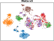
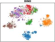
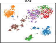
Fig. 4 uses T-SNE [42] to reveal the feature differences among MoCo-v3, DINO, iBOT, and Mugs, in which each color denotes a unique class. From the last subfigure, one can find that for one class, Mugs often divides it into several small clusters in the feature space, such as 6 clusters for brown, 4 for purple, 6 for red, and 5 for blue, and scatters these small clusters in a big class. This partially reveals multi-granular structures in the feature: classes are separately scattered, which corresponds to a group-level coarse granularity; several small scattered clusters in a class show a local-group-level fine granularity; and some separate instances in a cluster reveal an instance-level fine granularity. In contrast, MoCo-v3, DINO and iBOT often do not show this multi-granular feature structure. Hence, for some challenging classes denoted by green, red and purple colors, our Mugs can well distinguish them, while MoCo-v3, DINO and iBOT cannot. This is because instead of regarding the class as a whole, Mugs utilizes its multi-granular supervisions to consider the multi-granular (hierarchical) data semantic structures and divide the whole class into several easily-distinguishable clusters in the pretraining phase. Differently, MoCo-v3, DINO and iBOT ignore the multi-granular semantic structures and only uses one granular supervision which often could not well handle the challenging classes. Fig. 4 (a) further visualizes the self-attention of ViT-B/16. One can observe Mugs can well capture object shapes and thus their semantics. See more details and examples in Appendix 0.A.3.

Figure 4: T-SNE visualization of the learned feature by ViT-B/16. We show the fish classes in ImageNet-1K, i.e., the first six classes, including tench, goldfish, white shark, tiger shark, hammerhead, electric ray. See more examples in Appendix.

4.2 Results on downstream tasks

Due to limited space, we defer training and implementation details to Appendix.

Table 4: Classification accuracy (%) for transfer learning on six datasets.

Method	ViT-S/16						ViT-B/16
	Cif10	Cif100	INat18	INat19	Flwrs	Car	Cif10	Cif100	INat18	INat19	Flwrs	Car
Sup. [10]	99.0	89.5	70.7	76.6	98.2	92.1	99.0	90.8	73.2	77.7	98.4	92.1
BEiT [3]	98.6	87.4	68.5	76.5	96.4	92.1	99.0	90.1	72.3	79.2	98.0	94.2
MAE [28]	—	—	—	—	—	—	—	—	75.4	80.5	—	—
MoCo-v3 [18]	—	—	—	—	—	—	98.9	90.5	—	—	97.7	—
DINO [10]	99.0	90.5	72.0	78.2	98.5	93.0	99.1	91.7	72.6	78.6	98.8	93.0
iBOT [61]	99.1	90.7	73.7	78.5	98.6	94.0	99.2	92.2	74.6	79.6	98.9	94.3
Mugs (ours)	99.2	91.8	74.4	79.8	98.8	93.9	99.3	92.8	76.4	80.8	98.9	94.0

4.2.1 Transfer learning.

Here we investigate the transferability of the models pretrained by Mugs. Specifically, we pretrain the model on ImageNet-1K, and then fine-tune the pretrained backbone on various kinds of other datasets with same protocols and optimization settings in [10, 61]. Table 4 summarizes the classification accuracy, in which “Sup.” denotes the setting where we pretrain the backbone on ImageNet-1K in a supervised manner and then fine tune backbone on the corresponding dataset. Table 4 shows our Mugs surpasses SoTAs on the first five datasets and achieves comparable accuracy on the Car dataset.

4.2.2 Object detection & Instance segmentation.

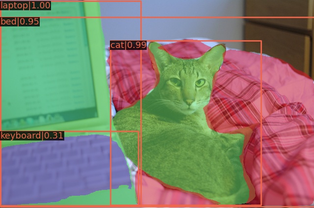
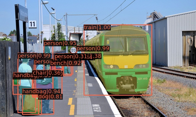
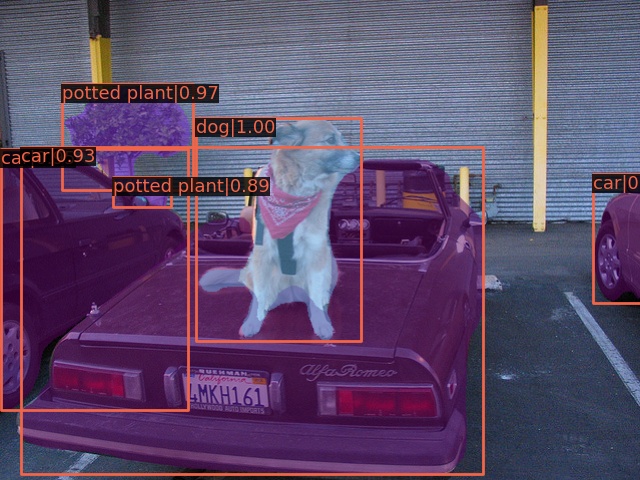
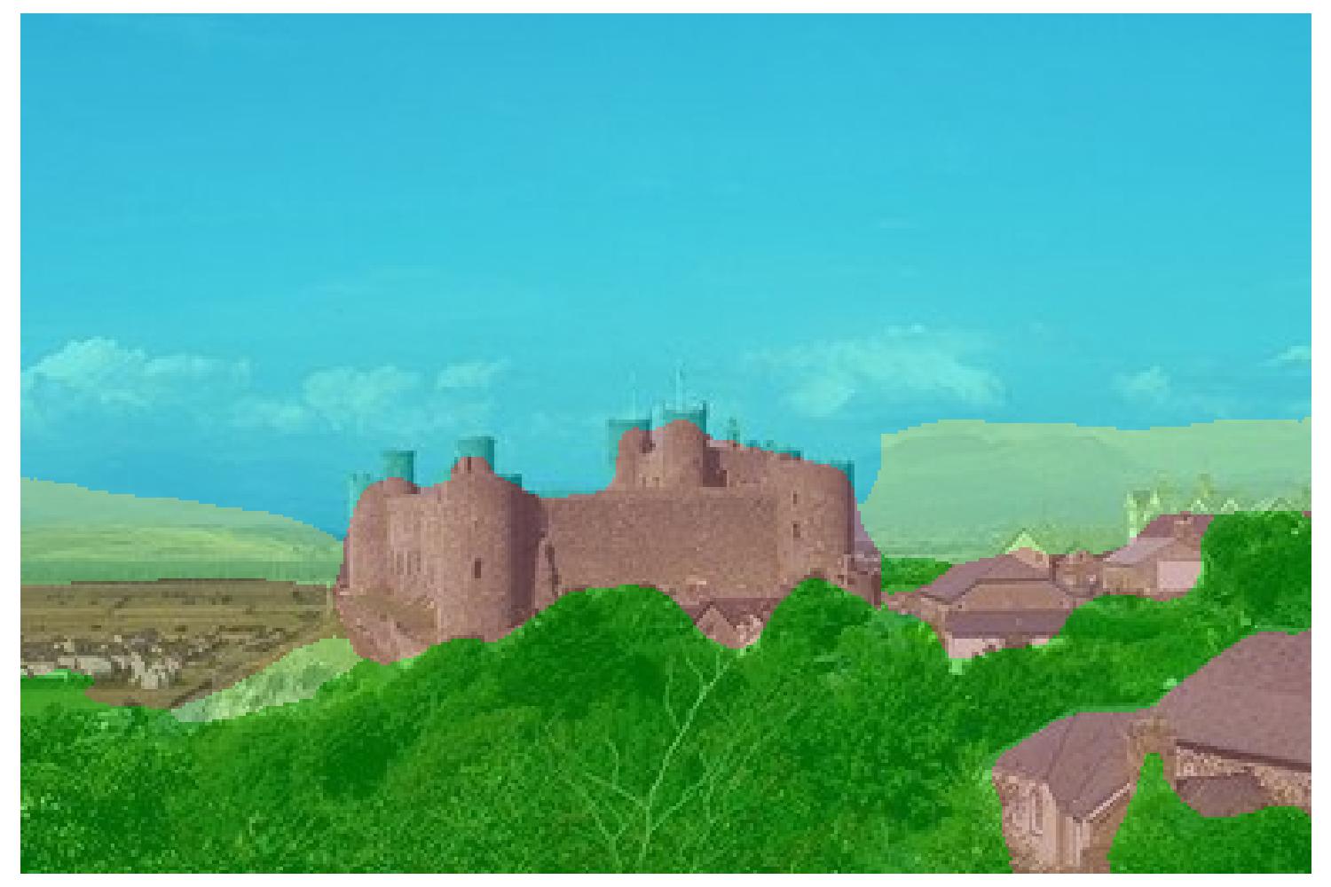
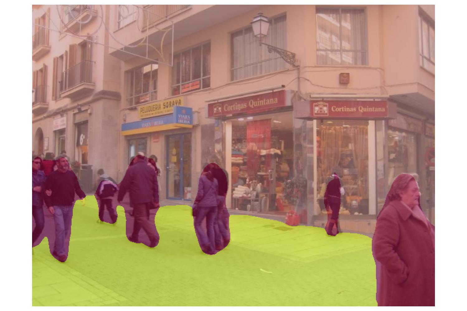
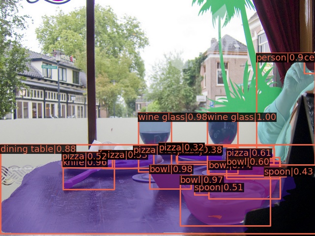
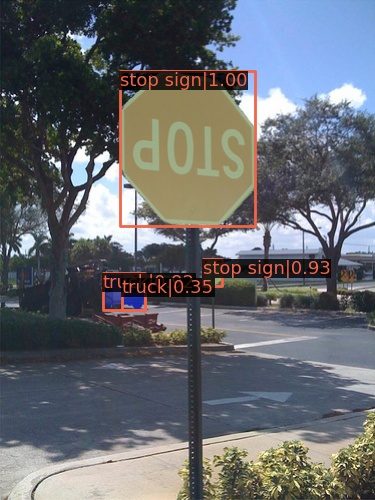
Now we evaluate Mugs on object detection and instance segmentation on COCO [38], in which both tasks emphasize the ability to locate and discriminate objects. For fairness, we use the same protocol in [61] which builds on Cascade Mask R-CNN [5, 31] to produce bounding boxes and instance masks simultaneously. See optimization settings in Appendix 0.B. Besides SSL approaches, e.g. MoBY [55], we also compare supervised baselines, Swin-T/7 [39] with similar model size as ViT-S/16. Table 6 shows that on detection, Mugs achieves 49.8 AP^b and makes 0.4 AP^b improvement over the runner-up, i.e. iBOT. Fig. 4 (b) shows that Mugs can accurately locate and classify objects in COCO. For instance segmentation, Mugs also surpasses all compared baselines and improves 0.4 AP^m over the best baseline.

(a) attention visualization			(b) object detection		(c) semantic segmentation

Figure 4: Visualization of pretrained ViT-B/16 (a) and ViT-S/16 (b) & (c) by Mugs. See more examples in Appendix. Best viewed in $3\times$ sized color pdf.

Table 5: ​​Object​ detection​ (Det.)​ &​ instance​ segmentation​ (ISeg.)​ on​ COCO​ &​ semantic​ seg.​ (SSeg.)​ on​ ADE20K.

	Arch.	Param.	Det.	ISeg.	SSeg.
			APb	APm	mIoU
Sup. [61]	Swin-T	29	48.1	41.7	44.5
MoBY [55]	Swin-T	29	48.1	41.5	44.1
Sup.  [61]	ViT-S/16	21	46.2	40.1	44.5
iBOT [61]	ViT-S/16	21	49.4	42.6	45.4
Mugs (ours)	ViT-S/16	21	49.8	43.0	47.4

Table 6: Video object segmentation with ViT-B/16 on the DAVIS-2017 video dataset.

	$(\mathcal{J}\&\mathcal{F})_{m}$	$\mathcal{J}_{m}$	$\mathcal{F}_{m}$
DINO [10]	62.3	60.7	63.9
iBOT [61]	62.4	60.8	64.0
Mugs	63.1	61.4	64.9

4.2.3 Semantic segmentation.

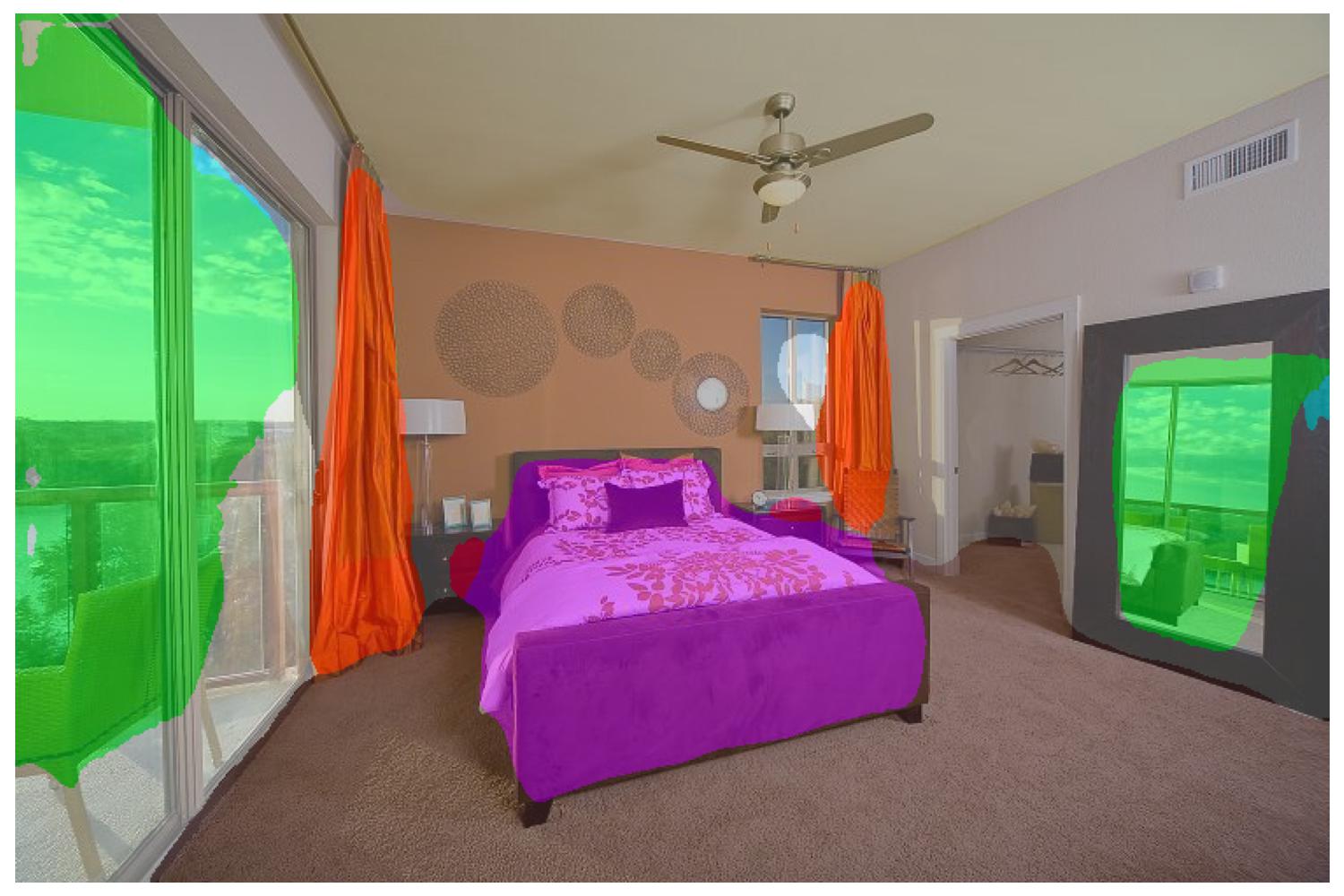
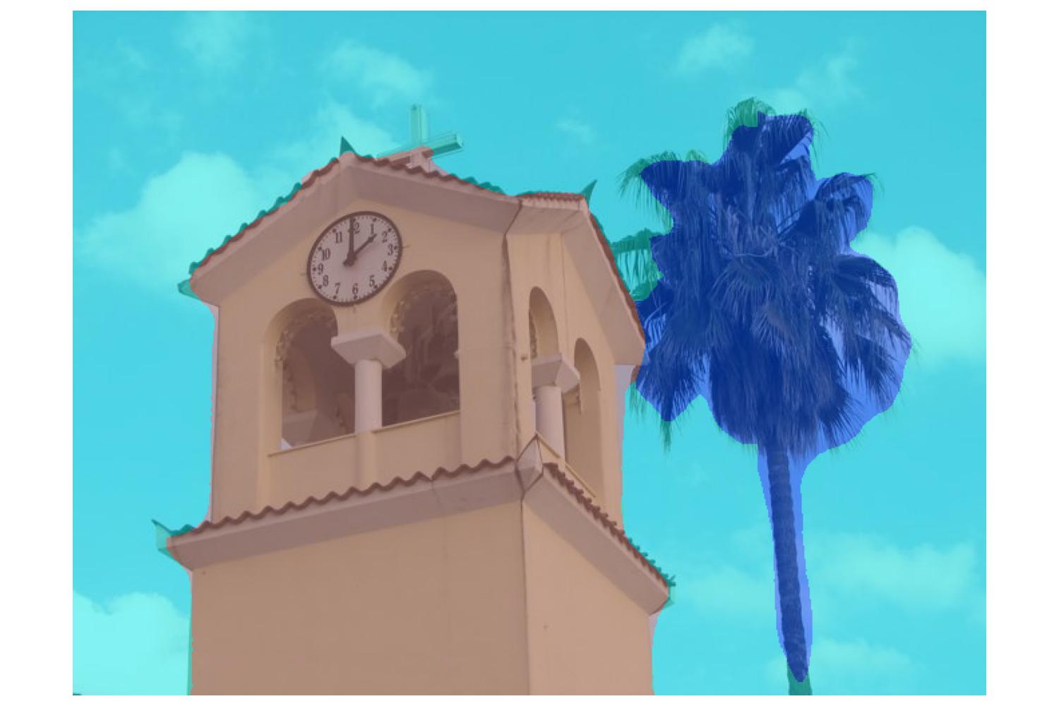
We transfer the pretrained model to semantic segmentation task on the ADE20K dataset [60]. Following [61], we stack the task layer in UPerNet [53] and fine-tune the whole backbone. Table 6 reports the mean intersection over union (mIoU) on all semantic categories. Mugs consistently outperforms the compared SoTAs by making significant 2.0 mIoU improvement. Fig. 4 (c) shows that Mugs can capture the object shape accurately.

4.2.4 Video object segmentation

via nearest neighbor retrieval. Besides images, we further evaluate the transferability of the frozen pretrained features on videos. Following DINO, we find nearest neighbors to segment objects in the video, since one can propagate segmentation masks via retrieving nearest neighbor between consecutive video frames [46]. Table 6 reports the mean region similarity $\mathcal{J}_{m}$ and mean contour-based accuracy $\mathcal{F}_{m}$ on the DAVIS-2017 video segmentation dataset [47] by using ViT-B/16. One can see that Mugs enjoys better feature transferability than DINO and iBOT even for video segmentation.

4.3 Ablation Study

Here we investigate the effects of each granular supervision in Mugs. Specifically, we train Mugs for 1,00 epochs on ImageNet-1K and report the linear probing accuracy in Table 7. One can observe that by independently removing each granular supervision, namely, the instance, local-group and group supervision, the performance of Mugs degenerates, which shows the benefit of each granular supervision, especially for the local-group supervision.

Next, we compare Mugs with DINO and iBOT under different augmentations and also show the effects of augmentations. Specifically, for the augmentation $\mathcal{\footnotesize{T}}^{\mbox{\scriptsize{s}}}$ in student network of Mugs/DINO/iBOT, we implement it by strong or weak augmentation mentioned at the beginning of Sec. 4; for augmentation $\footnotesize{\mathcal{T}}^{\mbox{\scriptsize{t}}}$ in teacher, we always use weak augmentation. See more implementation details in Appendix 0.B, especially for iBOT. We pretrain all methods for 1,00 epochs on ImageNet-1K. Table 8 shows four observations. 1) Under weak or strong augmentation, Mugs consistently outperforms DINO and iBOT. 2) For all three methods, strong augmentation slightly improves their performance under weak augmentation, showing the effectiveness of our strong augmentation technique on ViTs. 3) Mugs using weak augmentation surpasses iBOT that adopts both weak augmentation and random mask augmentation. 4) Under weak augmentation, Mugs improves 1.5% over DINO which means it is the multi-granular supervisions of Mugs that contributes this 1.5% improvement. Then by using strong augmentation, Mugs surpasses DINO using weak augmentation by 2.2%, showing strong augmentation only contributes 0.7% improvement over DINO. So compared with the strong augmentation technique, the multi-granular supervision framework of Mugs largely contributes to Mugs and is the key factor to the significant improvement of Mugs over DINO and iBOT.

Finally, we evaluate Mugs without multi-crop augmentation, i.e. only using two crops of size 224$\times$224 for pretraining. Table 9 in Appendix 0.A shows that Mugs also surpasses the SoTAs, including DINO and iBOT, on ViTs under the same setting, which also demonstrates the superiority of Mugs.

Table 7: Effects of the three granular supervisions in Mugs to the linear probing accuracy (%) on ImageNet-1K. $\mathcal{L}_{\text{instance}}$, $\mathcal{L}_{\text{local-group}}$ and $\mathcal{L}_{\text{group}}$ respectively denote the instance, local-group and group discrimination supervision.

Method	Mugs	Mugs w/o $\mathcal{L}_{\text{instance}}$	Mugs w/o $\mathcal{L}_{\text{local-group}}$	Mugs w/o $\mathcal{L}_{\text{group}}$
Acc (%)	76.4	75.8	75.3	75.7

Table 8: Augmentation effects to linear probing accuracy (%) on ImageNet-1K. $\dagger$ denotes that we replace vanilla augmentation in the method and run this variant.

weak aug.			strong aug.			weak aug.+random mask
DINO	iBOT†	Mugs	DINO†	iBOT†	Mugs	iBOT
74.2	74.9	75.7	74.7	75.4	76.4	75.3

5 Conclusion

In this work, we propose Mugs to learn multi-granular features via three complementary granular supervisions: instance discrimination supervision (IDS), local-group discrimination supervision (LGDS), and group discrimination supervision (GDS). IDS distinguishes different instances to learn fine-grained features. LGDS considers the local-group around an instance and then discriminates different local-groups to extract higher-level fine-grained features. GDS clusters similar samples and local-groups into one cluster to capture coarse-grained global group semantics. Experimental results have testified the advantages of Mugs.

Mugs: A Multi-Granular Self-Supervised Learning Framework (Supplementary File)

Pan Zhou^1∗   Yichen Zhou^1∗   Chenyang Si^1∗   Weihao Yu¹   Teck Khim Ng²   Shuicheng Yan¹

This supplementary document provides more additional experimental results and the pretraining & fine-tuning details for the ECCV’22 submission entitled “Mugs: A Multi-Granular Self-supervised Learning Framework”. It is structured as follows. Appendix 0.A provides more extra experimental results, including 1) the comparison among SoTAs without the multi-crop augmentation strategy in Appendix 0.A.1, 2) fine-tuning comparison on ViT-L/16 in Appendix 0.A.2, 3) more T-SNE clustering visualization results in Appendix 0.A.3, 4) more attention visualization results in Appendix 0.A.4, 5) more visualization results on object detection and segmentation in Appendix 0.A.5.

Appendix 0.B provides more experimental details for Sec. 4 in manuscript. Specifically, Appendix 0.B.1 gives more pretraining details, including implementations of weak and strong augmentations, loss construction under multi-crop setting, hyper-parameter settings for pretraining and the pretraining cost. Then Appendix 0.B.2 introduces more details for fine-tuning and semi-supervised learning in Sec. 4.1 in manuscript. Next, in Appendix 0.B.3, we present more details for downsteam tasks, including transfer learning, object detection & instance segmentation, and semantic segmentation. Finally, Appendix 0.B.4 tells us more implementation details of DINO and iBOT under weak and strong agumentation settings to complement Sec. 4.3 in manuscript.

Table 9: Linear probing accuracy (%) and k-NN accuracy (%) on ImageNet-1K without multi-crop augmentation (left) and with multi-crop augmentation (right). “Epo” is the effective pretraining epochs adjusted by number of views processed by the models following [61].

Method	Para.	Epo.	Lin.	k-NN
DINO	21	3200	73.7	70.0
iBOT	21	3200	76.2	72.4
Mugs	21	3200	76.9	73.1

Method	Para.	Epo.	Lin.	k-NN
DINO	21	3200	77.0	74.5
iBOT	21	3200	77.9	75.2
Mugs	21	3200	78.9	75.6

Appendix 0.A More Experimental Results

Due to space limitation, we defer more experimental results to this appendix. Here we first investigate the performance of Mugs without multi-crop augmentations which is widely used in several representative works, and further compare it with other methods, include iBOT and DINO under the same setting. Then we present more visualization results, including T-SNE clustering visualization, attention visualization of multi-heads in ViT, and object detection and segmentation visualization. We hope these visualization results can help readers intuitively understand the learnt features by Mugs.

0.A.1 Comparison w/o and w/ Multi-Crop Augmentation

Here we first investigate the performance of Mugs without the multi-crop augmentation which is widely used in several representative works, and further compare it with other SoTA methods, include iBOT and DINO under the same setting. Specifically, for Mugs without multi-crop augmentation, it only uses two 224-sized crops for pretraining. The left table in Table 9 reports the results of all compared methods without multi-crop augmentation, while the right one summarizes the results under multi-crop augmentation setting. By comparison, one can observe that without multi-crop augmentation, Mugs still consistently achieves the highest accuracy under both linear probing setting and KNN setting. Specifically, Mugs improves the runner-up, namely iBOT, by respectively $0.8\%$ and $0.5\%$ under linear probing and KNN evaluation settings. More importantly, we can observe that Mugs without multi-crop augmentation even achieves very similar results as DINO with multi-crop augmentation. All these results are consistent with those results in Table 1 in the manuscript, and well demonstrate the superiority of Mugs over previous state-of-the-arts.

Table 10: Fine-tuning classification accuracy (%) on ImageNet-1K. All methods are pretrained on ImageNet-1K. “Epo.” is the effective pretraining epochs adjusted by number of views processed by the models following [61].

	Method	ViT-L/16
		Epo.	Acc. (%)
	Supervised [49]	—	83.1
	BEiT [3]	800	85.2
reconstruction	MAE [28]	1600	85.9
	data2vec [2]	1600	86.6
	DINO [10]	—	—
contrastive or	iBOT [61]	1000	84.8
clustering	MoCo-v3 [18]	600	84.1
	Mugs (ours)	1000	85.2

0.A.2 Comparison under Fine-tuning Setting

In the manuscript, we already compare Mugs with state-of-the-art approaches on the ViT-S/16 and ViT-B/16 under the fine-tuning setting. Due to limited space, we defer the comparison among Mugs and others on ViT-L/16 into Table 10. This setting allows us to optimize the pretrained backbone with a linear classifier. Following BEiT [3], DINO and iBOT, we use AdamW optimizer with layer-wise learning rate decay to train ViT-L for 50 epochs on ImageNet-1K. On ViT-L, Mugs achieves 85.2% top-1 accuracy, and surpasses all contrastive learning and clustering learning methods. One can also observe that on ViT-L, most of the reconstruction methods achieves higher accuracy than constrictive or clustering learning approaches, including iBOT and our Mugs. There are two possible reasons. Firstly, the reconstruction methods use much more computations for pretraining than constrictive or clustering learning approaches. Specifically, the reconstruction family always use 224$\times$224-sized images to pretrain the model, while constrictive or clustering learning approaches uses multi-crop augmentations which contains two 224-sized images and ten 96-sized images. Since “Epo.” in Table 10 is the effective pretraining epochs adjusted by number of views processed by the models [61] which means each $96$-sized image equals to one $224$-sized image in terms of the defined “epochs”, with the same pretraining epochs, the computation cost of the reconstruction approaches is much more. Actually, from Table 10, the reconstruction methods have much more effective pretraining epochs than constrictive or clustering learning approaches, e.g. 1600 epochs in data2vec v.s. 1000 epochs in iBOT & Mugs, which further increases the training cost. Secondly, for large models, using small-sized images, e.g. ten 96-sized images in multi-crop augmentations, may lead to overfitting issue in contrastive or clustering learning approaches. Specifically, from Table 1 in manuscript and Table 10 here, once can observe that on relatively small models, such as ViT-S and ViT-B, SoTA contrastive learning or clustering methods, such as Mugs and iBOT, outperform the reconstruction methods, even though the formers have much less pretraining cost as mentioned above. But on large models, e.g. ViT-L, the superiority of SoTA contrastive or clustering learning methods disappears. One possible reason for these inconsistent observation is that large model needs more pretraining epochs for learning semantic features, and could suffer from over-fitting problem when using 96-sized crops, since 1) large model is capable to memory all images as demonstrated in many works; and 2) 96-sized crops may contain incomplete semantics of the vanilla image and lead to over-fitting issue, especially under insufficient pretraining epochs. Note, as explained at the end of Sec. 2 in manuscript, this fine-tuning setting needs much higher extra training cost, and also destroys model compatibility for deployment. Therefore, in this work, we do not further push Mugs’s limits on the large models which needs huge training cost as the reconstruction methods.

(a) T-SNE visualization of 19 classes of insects, e.g. beetle, butterfly, stick, and cricket.

(b) T-SNE visualization of 20 classes of various monkeys, e.g. gibbon, siamang, patas, and gorilla.

(c) T-SNE visualization of 17 classes of various birds, e.g. junco, robin, jay, cock, and ostrich.

Figure 5: More T-SNE visualization of the learned features by ViT-B/16 trained by our Mugs. Best viewed in color pdf file.

0.A.3 More T-SNE Visualization Results

Same with Fig. 4 in the manuscript, here we use T-SNE [42] to reveal the feature differences among MoCo-v3, DINO, iBOT, and Mugs in Fig. 5. By comparison, Mugs often can scatter the samples from different classes more separately, while keeping the samples in the same class close in the feature space. This could means that our Mugs can better distinguish different classes than MoCo-v3, DINO and iBOT, and thus shows higher performance. The potential reason behind this observation is explained in manuscript. That is, instead of regards the class as a whole, Mugs utilizes its multi-granular supervisions to consider the multi-granular (hierarchical) data semantic structures and divides the whole class into several clusters for easily discriminating in the pretraining phase. Differently, MoCo-v3, DINO and iBOT ignore the multi-granular semantic structures and only uses one granular supervision which often could not well handle the challenging classes.

Figure 6: Self-attention visualization of ViT-B/16 pretrained by our Mugs. The images from left to right respectively denote the vanilla image, the overall self-attention score of all 12 heads in ViT-B, and the individual self-attention score of 12 heads. Best viewed in color pdf file.

0.A.4 More Attention Visualization Results

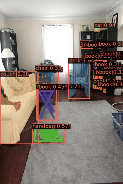
Here same with Fig. 4 in the manuscript, we visualize more self-attention map of the 12 self-attention heads in ViT-B/16 pretrained by Mugs in Fig. 6. The first column denotes the vanilla images, while each column of the last 12 columns denote the self-attention score maps of each individual head. The second column combines the 12 self-attention score maps from 12 heads into one, and also sets a threshold to remove some noises via only keeping top attention score. From these visualizations, one can observe that by using Mugs for pretraining, the overall self-attention of 12 heads can capture the object shapes very well. For example, from the first bird image, it is even hard for human to get the bird location at the first glance, due to the similar color of the bird and the flowers. But the ViT-B/16 pretrained by Mugs still can well locate the bird and also capture the bird shape. Moreover, one can also compare the attention visualization of Mugs with state-of-the-arts, e.g. iBOT. In iBOT [61], Fig. 18 in their appendix also visualizes the self-attention map. By comparison, the model pretrained by Mugs can better separate the object from background. These results testify that ViT-B/16 pretrained by Mugs can capture semantics in data even without any manual labels.

Figure 7: Object detection visualization of ViT-B/16 pretrained by Mugs. Best viewed in color pdf file.

Figure 8: Semantic segmentation visualization of ViT-B/16 pretrained by Mugs. Best viewed in color pdf file.

0.A.5 More Visualization Results on Object Detection and Semantic Segmentation

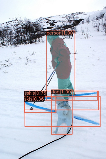
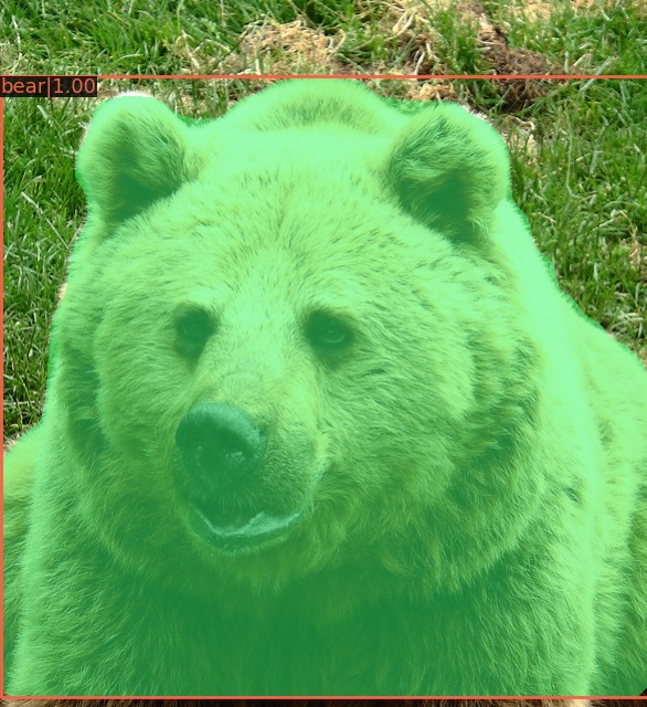
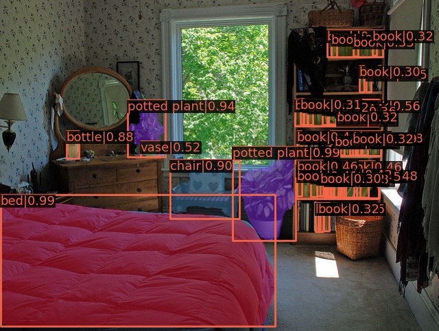
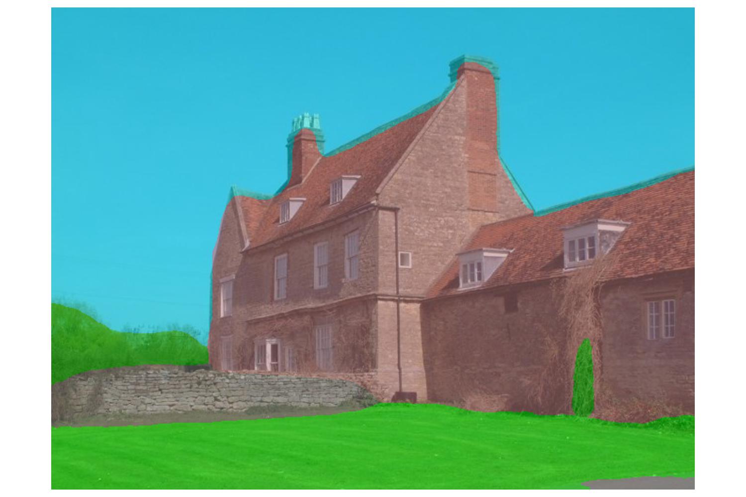
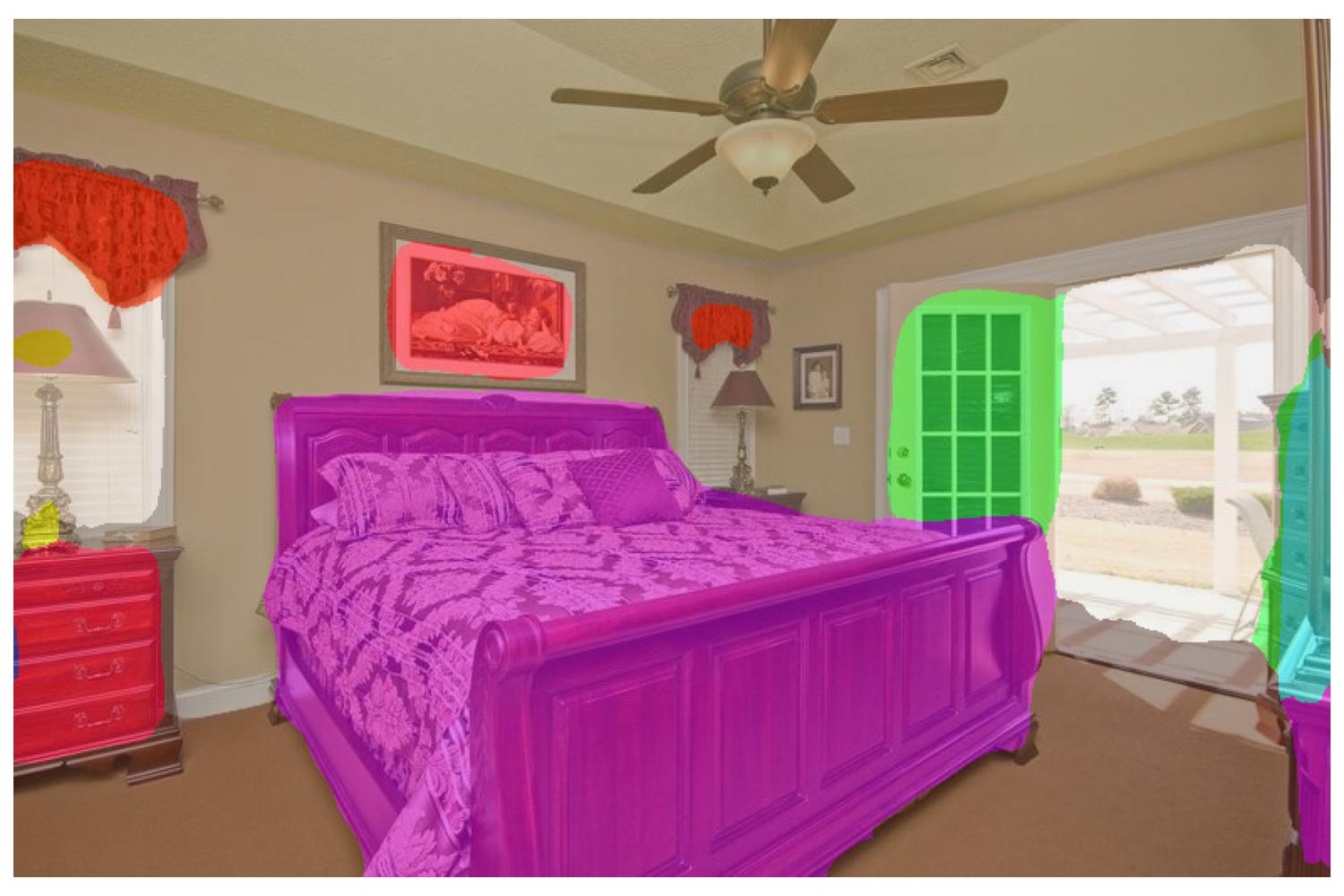
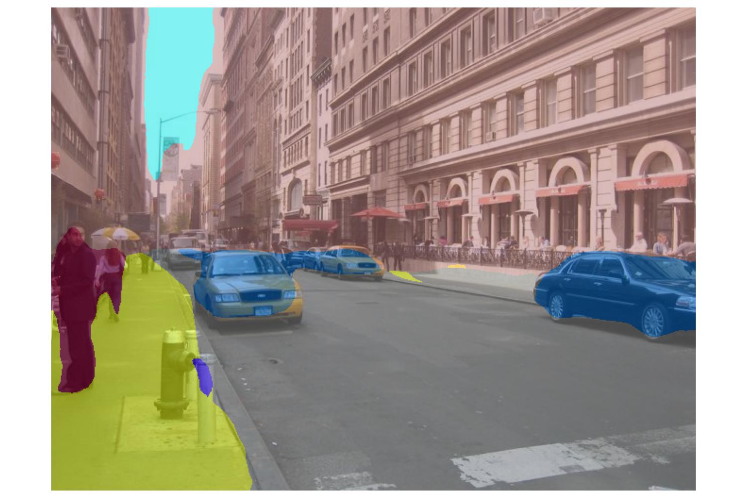
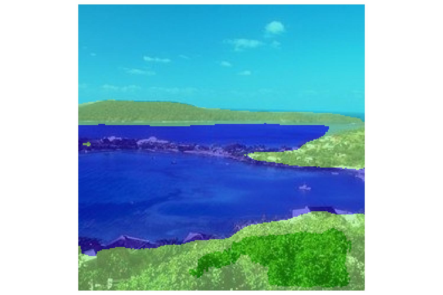
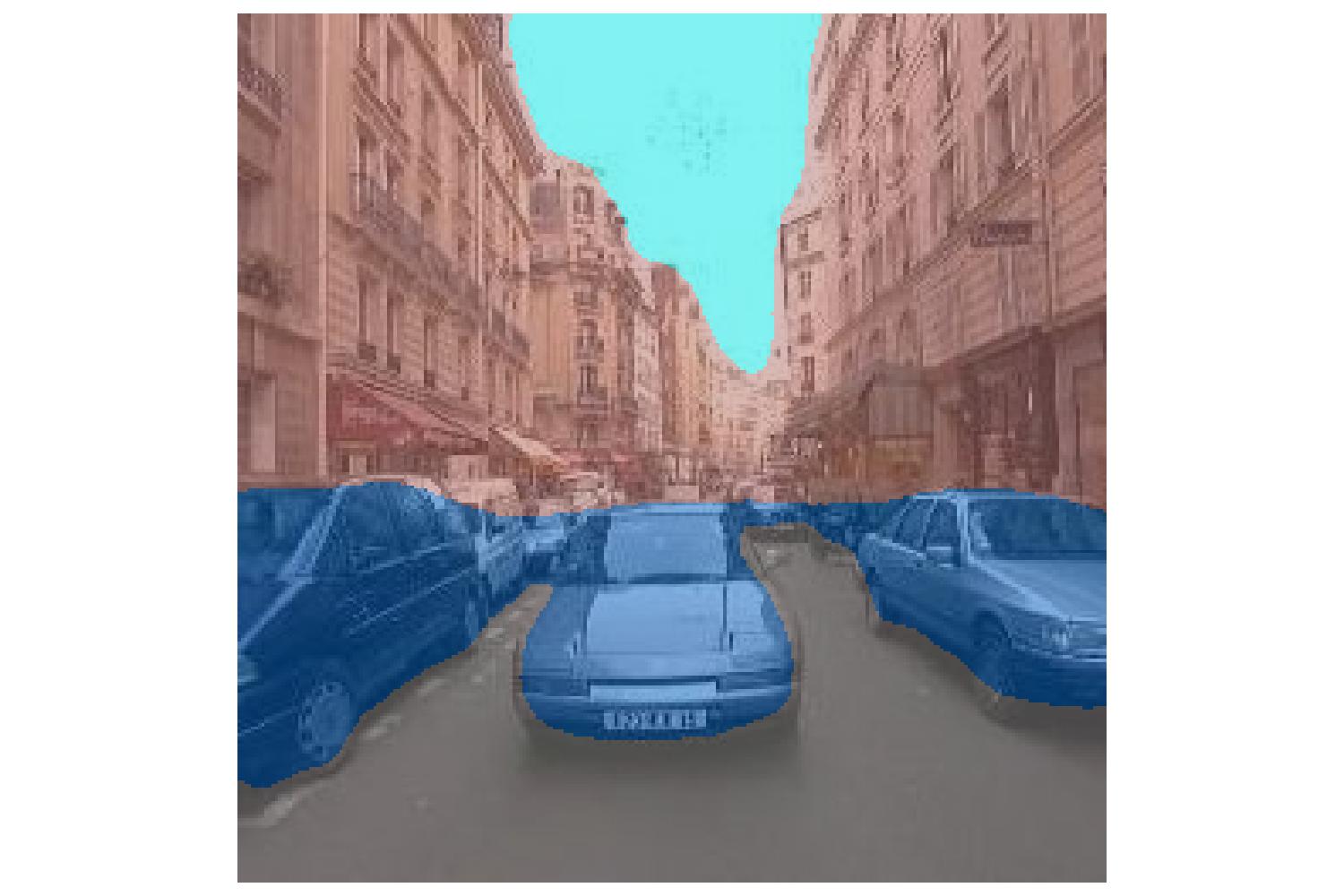
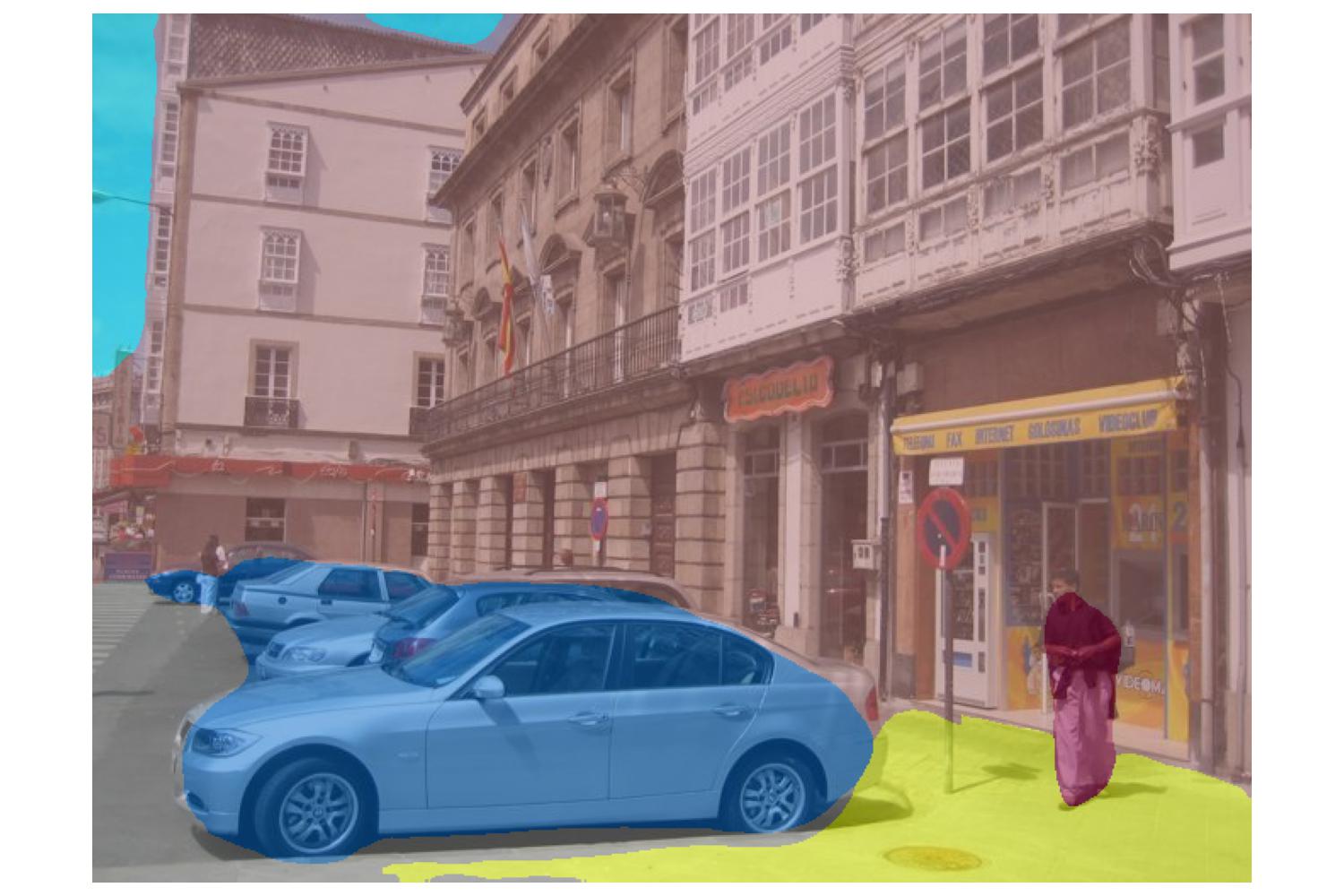
In the manuscript, we already provide some object detection and segmentation examples in Fig. 4. Here we give more examples. Fig. 7 shows more object detection examples on the COCO datasets, where we use the ViT-B/16 pretrained by our Mugs. From these results, one can observe that Mugs not only accurately locate the objects in the images but also precisely recognizes these objects. For semantic segmentation on ADE20K, Fig. 8 visualizes more examples. We also can find that Mugs can capture the object shape accurately and thus well captures the semantics of an image.

Appendix 0.B More Experimental details

Due to space limitation, we defer more experimental details to this section. Here we first provide more details for pretraining. Then we present the experimental details for various kinds of downstream tasks. Finally, we also give the details for ablation study.

0.B.1 More Details for Pretraining

0.B.1.1 Augmentation.

Here the weak augmentation in our teacher backbone refers to the augmentations used in many SSL works, e.g. DINO [10], which includes random crop, color jitter, Gaussian noise, horizontal flipping and gray scaling. The hyper-parameters in these augmentation operations are the same with those in DINO [10]. The strong augmentation in our student backbone is the combination of AutoAugment [19] used in DeiT [49] and the above weak augmentation. Specifically, for each image, with probability 0.5, we use AutoAugment [19] to augment it; otherwise, we use weak augmentation to crop it. We use this sampling strategy to avoid training collapse while keeping sufficient data diversity. Following DINO and iBOT, we always set the global crop scale as $[0.25,1]$ and local crop scale as $[0.05,0.25].$

0.B.1.2 Loss for multi-crop setting.

Following conventional multi-crop setting [9, 10, 61], we crop each image into 2 large crops of size $224$ and 10 extra small crops of size $96$. Then to construct the overall pretraining loss 6 in manuscript, we regard one large crop as $\bm{x}_{1}$ and respectively take the remaining 11 crops as $\bm{x}_{2}$. Then symmetrically, we view another large crop as $\bm{x}_{1}$ and respectively take the remaining 11 crops as $\bm{x}_{2}$. Finally, we average these loss to obtain the overall training loss.

0.B.1.3 Hyper-parameter settings for Pretraining.

For all experiments, we use AdamW optimizer [41] with a momentum of 0.9 and a cosine learning rate schedule [40]. We also linearly warm up the learning rate at the first 10 epochs from $10^{-6}$ to its base value, and then decay it with a cosine schedule [40]. For ViT-S and ViT-B, we use a minibatch size of 1024, a base learning rate of $8\times 10^{-4}$, and a weight decay of 0.1. For ViT-L, due to our limited computational resource, we use a minibatch size of 640, a base learning rate of $1.5\times 10^{-4}$, and a weight decay of 0.08. For all experiments, the learning rate of the patch embedding layer is 5$\times$ smaller than the base learning rate. This strategy is demontrated to be useful for stabling training in MoCo-v3 [18]. For drop path rate, we set it as 0.1/0.2/0.4 for ViT-S/B/L respectively. We set clip gradient as 3.0 for ViT-S/B and 0.3 for ViT-L. For Mugs, we follow MoCo to set $\tau_{\mbox{\scriptsize{in}}}=\tau_{\mbox{\scriptsize{lg}}}=0.2$ in the infoNCE loss, and follow DINO to set $\tau_{\mbox{\scriptsize{g}}}^{\prime}=0.1$ and linearly warm up $\tau_{\mbox{\scriptsize{g}}}$ from $0.04$ to $0.07$. We set the neighbor number $k=8$, and set $\rho=0.9$ to estimate the center $\bm{p}_{\mbox{\scriptsize{ema}}}$ in group discrimination. All these settings are almost the same as DINO for simplicity which reduces hyper-parameter tuning and saves computational budget.

0.B.1.4 Pretraining Cost.

Mugs takes about $27$ hours with $8$ A100 GPUs for $100$ pretraining epochs on ViT-S/16. This means that Mugs has almost the same training cost with DINO, since our projection/prediction heads and transformers $g_{\mbox{\scriptsize{transformer}}}$ are much smaller than the backbone. For ViT-B/16, Mugs needs about 24 hours on 16 A100 GPUs for $100$ pretraining epochs. To training 100 epochs on ViT-L/16, Mugs takes about 48 hours on 40 A100 GPUs. For ViT-B and ViT-L, it is hard for us to compare with DINO, since it does not report the training time.

0.B.2 More Training Details for Evaluation on ImageNet-1K

0.B.2.1 Fine-tuning.

As mentioned in manuscript, we follow BEiT [3], DINO and iBOT, and use AdamW optimizer with layer-wise learning rate decay to train ViT-S/ViT-B/ViT-L for 200/100/50 epochs on ImageNet-1K. We set layer-wise learning rate decay as 0.55 and learning rate $1.2\times 10^{-3}$ for both ViT-S and ViT-B. For ViT-L, we use layer-wise learning rate decay 0.75 and learning rate $8.0\times 10^{-4}$. For drop path rate, we set it as 0.1/0.2/0/3 for ViT-S/ ViT-B/ViT-L respectively. All these hyper-parameters are around at the suggested ones in BEiT and iBOT.

0.B.2.2 Semi-supervised learning.

Following DINO and iBOT, we consider two settings: 1) training a logistic regression classifier on frozen features; and 2) fine-tuning the whole pretrained backbone. For logistic regression classifier, we use AdamW optimizer with total minibatch size 1024 and weight decay 0.05, under both 1% and 10% training data settings. We sweep the learning rate $\{0.03,0.06,$ $0.10,0.2\}$. For fine-tuning 1000 epochs on ViT-S/16, we also use AdamW optimizer with total minibatch size 1024 and weight decay 0.05 under both 1% and 10% training data settings. We respectively set learning rate as $2\times 10^{-6}$ and $5\times 10^{-6}$ for 1% and 10% training data.

0.B.3 More Details for Downsteam Tasks

0.B.3.1 Transfer learning.

We pretrain the model on ImageNet-1K, and then fine-tune the pretrained backbone on various kinds of other datasets with same protocols and optimization settings in DINO and iBOT. Specifically, following DINO and iBOT, for both ViT-S and ViT-B, we always use AdamW optimizer with a minibatch size of 768. We fine-tune the pretrained model 360 epochs on INat₁₈ and INat₁₉, and 1000 epochs on Cif₁₀, Cif₁₀₀, Flwrs and Car. For all datasets, we sweep the learning rate $\{7.5\times 10^{-6},1.5\times 10^{-5},3.0\times 10^{-5},7.5\times 10^{-5},1.5\times 10^{-4}\}$. For we set weight decay as $2\times 10^{-2}$ for CIFAR10 and CIFAR100 on ViT-B, and use a weight decay of $5\times 10^{-2}$ for all remaining experiments. For example, on the INat₁₈ dataset, we use a learning rate of $3.0\times 10^{-5}$/$1.5\times 10^{-5}$ for ViT-S/ViT-B; on the INat₁₉ dataset, we set learning rate as $7.5\times 10^{-5}$/$3.0\times 10^{-5}$ for ViT-S/ViT-B. For more hyper-parameters, please refer to the hyper-parameter configure file in our released code.

0.B.3.2 Object detection & Instance segmentation.

For fairness, we follow DINO and iBOT, and fine-tune the pretrained backbone via a multi-scale strategy, namely resizing image at different scales. Please refer to iBOT for more details. We use AdamW optimizer with a learning rate of $2\times 10^{-4}$, a weight decay of $0.05$ to fine-tune with $1\times$ schedule, i.e. 12 epochs with the learning rate decayed by $10\times$ at epochs $9$ and $11$. We sweep a layer decay rate of {$0.65$, $0.75$, $0.8$, $0.9$} and finally choose 0.8 because of its good performance. For test, we do not use multi-scale strategy.

0.B.3.3 Semantic segmentation.

For semantic segmentation, we follow DINO and iBOT, and fine-tune the pretrained backbone, and fine-tune the pretrained backbone by using $512\times 512$-sized images for $1.6\times 10^{4}$ iterations. We use AdamW optimizer with a learning rate of $2\times 10^{-4}$, a weight decay of $0.05$ and a layer decay rate of $0.9$ to fine-tune. For this task, we do not use any multi-scale strategy for training and test. We sweep the learning rate $\{2\times 10^{-5},3\times 10^{-5},4\times 10^{-5},5\times 10^{-5}\}$ and finally choose $3\times 10^{-5}$ because of its good performance.

0.B.4 More details for Ablation Study

Here we provide the implementation details for DINO and iBOT under different augmentations. As mentioned in Sec. 4.3 in the manuscript, for the augmentation $\mathcal{\footnotesize{T}}^{\mbox{\scriptsize{s}}}$ in student network of Mugs/DINO/iBOT, we implement it by strong or weak augmentation as mentioned at the beginning of Sec. 4; for augmentation $\footnotesize{\mathcal{T}}^{\mbox{\scriptsize{t}}}$ in teacher, we always use weak augmentation.

We first consider weak augmentation setting. For DINO, there is no any change, since its vanilla version uses the weak augmentation. For Mugs, we only replace the strong augmentation used in the student network with the weak augmentation. For iBOT, it has two losses, the proposed masked image modeling (MIM) loss and the clustering loss in DINO. To construct the MIM loss, iBOT needs to randomly mask the patches of input in the student network. But to build the clustering loss, it actually does not require random masks on input patches, but still uses the random masks in practice which actually increases the data augmentations for clustering loss. In this case, for fair comparison, we remove the random masks and only perform weak augmentation to construct the clustering loss in iBOT. Note, we still preserve the random masks for MIM loss to ensure MIM is the vanilla one in iBOT.

We then consider strong augmentation setting. For DINO, we only replace the weak augmentation used in the student network with our strong augmentation. For iBOT, same as the above for weak augmentation, we does not change the augmentation in MIM loss. But for building the clustering loss, we also remove the random masks and only perform strong augmentation.

References

- [1] Bachman, P., Hjelm, R., Buchwalter, W.: Learning representations by maximizing mutual information across views. In: Proc. Conf. Neural Information Processing Systems. pp. 15535–15545 (2019)
- [2] Baevski, A., Hsu, W.N., Xu, Q., Babu, A., Gu, J., Auli, M.: Data2vec: A general framework for self-supervised learning in speech, vision and language. arXiv preprint arXiv:2202.03555 (2022)
- [3] Bao, H., Dong, L., Wei, F.: Beit: Bert pre-training of image transformers. arXiv preprint arXiv:2106.08254 (2021)
- [4] Bautista, M., Sanakoyeu, A., Tikhoncheva, E., Ommer, B.: Cliquecnn: Deep unsupervised exemplar learning. In: Proc. Conf. Neural Information Processing Systems. pp. 3846–3854 (2016)
- [5] Cai, Z., Vasconcelos, N.: Cascade R-CNN: High quality object detection and instance segmentation. tpami (2019)
- [6] Caron, M., Bojanowski, P., Joulin, A., M. Douze, M.: Deep clustering for unsupervised learning of visual features. In: Proc. European Conf. Computer Vision. pp. 132–149 (2018)
- [7] Caron, M., Misra, I., Mairal, J., Goyal, P., Bojanowski, P., Joulin, A.: Unsupervised learning of visual features by contrasting cluster assignments. In: Proc. Conf. Neural Information Processing Systems (2020)
- [8] Caron, M., Bojanowski, P., Joulin, A., Douze, M.: Deep clustering for unsupervised learning of visual features. In: Proceedings of the European Conference on Computer Vision (ECCV). pp. 132–149 (2018)
- [9] Caron, M., Misra, I., Mairal, J., Goyal, P., Bojanowski, P., Joulin, A.: Unsupervised learning of visual features by contrasting cluster assignments. arXiv preprint arXiv:2006.09882 (2020)
- [10] Caron, M., Touvron, H., Misra, I., Jégou, H., Mairal, J., Bojanowski, P., Joulin, A.: Emerging properties in self-supervised vision transformers. arXiv preprint arXiv:2104.14294 (2021)
- [11] Chen, T., Kornblith, S., Norouzi, M., Hinton, G.: A simple framework for contrastive learning of visual representations. In: Proc. Int’l Conf. Machine Learning (2020)
- [12] Chen, T., Kornblith, S., Swersky, K., Norouzi, M., Hinton, G.: Big self-supervised models are strong semi-supervised learners. In: Proc. Conf. Neural Information Processing Systems (2020)
- [13] Chen, T., Kornblith, S., Norouzi, M., Hinton, G.: A simple framework for contrastive learning of visual representations. In: III, H.D., Singh, A. (eds.) Proceedings of the 37th International Conference on Machine Learning. Proceedings of Machine Learning Research, vol. 119, pp. 1597–1607. PMLR (13–18 Jul 2020), https://proceedings.mlr.press/v119/chen20j.html
- [14] Chen, T., Kornblith, S., Swersky, K., Norouzi, M., Hinton, G.: Big self-supervised models are strong semi-supervised learners. arXiv preprint arXiv:2006.10029 (2020)
- [15] Chen, X., Fan, H., Girshick, R., He, K.: Improved baselines with momentum contrastive learning. arXiv preprint arXiv:2003.04297 (2020)
- [16] Chen, X., Fan, H., Girshick, R., He, K.: Improved baselines with momentum contrastive learning. arXiv preprint arXiv:2003.04297 (2020)
- [17] Chen, X., He, K.: Exploring simple siamese representation learning. In: Proceedings of the IEEE/CVF Conference on Computer Vision and Pattern Recognition. pp. 15750–15758 (2021)
- [18] Chen, X., Xie, S., He, K.: An empirical study of training self-supervised vision transformers. arXiv preprint arXiv:2104.02057 (2021)
- [19] Cubuk, E.D., Zoph, B., Mane, D., Vasudevan, V., Le, Q.V.: Autoaugment: Learning augmentation policies from data. arXiv preprint arXiv:1805.09501 (2018)
- [20] Dalal, N., Triggs, B.: Histograms of oriented gradients for human detection. In: 2005 IEEE computer society conference on computer vision and pattern recognition (CVPR’05). vol. 1, pp. 886–893. Ieee (2005)
- [21] Deng, J., Dong, W., Socher, R., Li, L.J., Li, K., Fei-Fei, L.: Imagenet: A large-scale hierarchical image database. In: 2009 IEEE conference on computer vision and pattern recognition. pp. 248–255. Ieee (2009)
- [22] Dong, X., Bao, J., Zhang, T., Chen, D., Zhang, W., Yuan, L., Chen, D., Wen, F., Yu, N.: Peco: Perceptual codebook for bert pre-training of vision transformers. arXiv preprint arXiv:2111.12710 (2021)
- [23] Dosovitskiy, A., Beyer, L., Kolesnikov, A., Weissenborn, D., Zhai, X., Unterthiner, T., Dehghani, M., Minderer, M., Heigold, G., Gelly, S., et al.: An image is worth 16x16 words: Transformers for image recognition at scale. arXiv preprint arXiv:2010.11929 (2020)
- [24] Grill, J., Strub, F., Altché, F., Tallec, C., Richemond, P., Buchatskaya, E., Doersch, C., Pires, B., Guo, Z., Azar, M.: Bootstrap your own latent: A new approach to self-supervised learning. In: Proc. Conf. Neural Information Processing Systems (2020)
- [25] Grill, J.B., Strub, F., Altché, F., Tallec, C., Richemond, P.H., Buchatskaya, E., Doersch, C., Pires, B.A., Guo, Z.D., Azar, M.G., et al.: Bootstrap your own latent: A new approach to self-supervised learning. arXiv preprint arXiv:2006.07733 (2020)
- [26] Hadsell, R., Chopra, S., LeCun, Y.: Dimensionality reduction by learning an invariant mapping. In: Proc. IEEE Conf. Computer Vision and Pattern Recognition. vol. 2, pp. 1735–1742. IEEE (2006)
- [27] He, K., Fan, H., Wu, Y., Xie, S., Girshick, R.: Momentum contrast for unsupervised visual representation learning. In: Proc. IEEE Conf. Computer Vision and Pattern Recognition. pp. 9729–9738 (2020)
- [28] He, K., Chen, X., Xie, S., Li, Y., Dollár, P., Girshick, R.: Masked autoencoders are scalable vision learners. arXiv preprint arXiv:2111.06377 (2021)
- [29] He, K., Chen, X., Xie, S., Li, Y., Dollár, P., Girshick, R.: Masked autoencoders are scalable vision learners. arXiv preprint arXiv:2111.06377 (2021)
- [30] He, K., Fan, H., Wu, Y., Xie, S., Girshick, R.: Momentum contrast for unsupervised visual representation learning. In: Proceedings of the IEEE/CVF Conference on Computer Vision and Pattern Recognition. pp. 9729–9738 (2020)
- [31] He, K., Gkioxari, G., Dollár, P., Girshick, R.: Mask R-CNN. In: iccv (2017)
- [32] Hjelm, R., Fedorov, A., Lavoie-Marchildon, S., Grewal, K., Bachman, P., Trischler, A., Bengio, Y.: Learning deep representations by mutual information estimation and maximization. arXiv preprint arXiv:1808.06670 (2018)
- [33] Huang, J., Dong, Q., Gong, S., Zhu, X.: Unsupervised deep learning by neighbourhood discovery. arXiv preprint arXiv:1904.11567 (2019)
- [34] Komodakis, N., Gidaris, S.: Unsupervised representation learning by predicting image rotations (2018)
- [35] Li, J., Zhou, P., Xiong, C., Socher, R., Hoi, S.C.: Prototypical contrastive learning of unsupervised representations. In: Int’l Conf. Learning Representations (2021)
- [36] Li, Z., Chen, Z., Yang, F., Li, W., Zhu, Y., Zhao, C., Deng, R., Wu, L., Zhao, R., Tang, M., et al.: Mst: Masked self-supervised transformer for visual representation. Advances in Neural Information Processing Systems 34 (2021)
- [37] Lin, S., Zhou, P., Hu, Z., Wang, S., Zhao, R., Zheng, Y., Lin, L., Xing, E., Liang, X.: Prototypical graph contrastive learning. arXiv preprint arXiv:2106.09645 (2021)
- [38] Lin, T.Y., Maire, M., Belongie, S., Hays, J., Perona, P., Ramanan, D., Dollár, P., Zitnick, C.L.: Microsoft coco: Common objects in context. In: eccv (2014)
- [39] Liu, Z., Lin, Y., Cao, Y., Hu, H., Wei, Y., Zhang, Z., Lin, S., Guo, B.: Swin transformer: Hierarchical vision transformer using shifted windows. arXiv preprint arXiv:2103.14030 (2021)
- [40] Loshchilov, I., Hutter, F.: Sgdr: Stochastic gradient descent with warm restarts. arXiv preprint arXiv:1608.03983 (2016)
- [41] Loshchilov, I., Hutter, F.: Fixing weight decay regularization in adam (2018)
- [42] Van der Maaten, L., Hinton, G.: Visualizing data using t-sne. Journal of machine learning research 9(11) (2008)
- [43] Noroozi, M., Favaro, P.: Unsupervised learning of visual representations by solving jigsaw puzzles. In: Proc. European Conf. Computer Vision. pp. 69–84. Springer (2016)
- [44] Oord, A., Li, Y., Vinyals, O.: Representation learning with contrastive predictive coding. arXiv preprint arXiv:1807.03748 (2018)
- [45] Oord, A.v.d., Li, Y., Vinyals, O.: Representation learning with contrastive predictive coding. arXiv preprint arXiv:1807.03748 (2018)
- [46] Philbin, J., Chum, O., Isard, M., Sivic, J., Zisserman, A.: Lost in quantization: Improving particular object retrieval in large scale image databases. In: 2008 IEEE conference on computer vision and pattern recognition. pp. 1–8. IEEE (2008)
- [47] Pont-Tuset, J., Perazzi, F., Caelles, S., Arbeláez, P., Sorkine-Hornung, A., Van Gool, L.: The 2017 davis challenge on video object segmentation. arXiv preprint arXiv:1704.00675 (2017)
- [48] Tian, Y., Sun, C., Poole, B., Krishnan, D., Schmid, C., Isola, P.: What makes for good views for contrastive learning? Advances in Neural Information Processing Systems 33, 6827–6839 (2020)
- [49] Touvron, H., Cord, M., Douze, M., Massa, F., Sablayrolles, A., Jégou, H.: Training data-efficient image transformers & distillation through attention. In: International Conference on Machine Learning. pp. 10347–10357. PMLR (2021)
- [50] Wang, T., Isola, P.: Understanding contrastive representation learning through alignment and uniformity on the hypersphere. In: Proc. Int’l Conf. Machine Learning (2020)
- [51] Wei, C., Fan, H., Xie, S., Wu, C.Y., Yuille, A., Feichtenhofer, C.: Masked feature prediction for self-supervised visual pre-training. arXiv preprint arXiv:2112.09133 (2021)
- [52] Wu, Z., Xiong, Y., Yu, S., Lin, D.: Unsupervised feature learning via non-parametric instance discrimination. In: Proc. IEEE Conf. Computer Vision and Pattern Recognition. pp. 3733–3742 (2018)
- [53] Xiao, T., Liu, Y., Zhou, B., Jiang, Y., Sun, J.: Unified perceptual parsing for scene understanding. In: eccv (2018)
- [54] Xie, S., Girshick, R., Dollár, P., Tu, Z., He, K.: Aggregated residual transformations for deep neural networks. In: Proc. IEEE Conf. Computer Vision and Pattern Recognition. pp. 1492–1500 (2017)
- [55] Xie, Z., Lin, Y., Yao, Z., Zhang, Z., Dai, Q., Cao, Y., Hu, H.: Self-supervised learning with swin transformers. arXiv preprint arXiv:2105.04553 (2021)
- [56] Xie, Z., Zhang, Z., Cao, Y., Lin, Y., Bao, J., Yao, Z., Dai, Q., Hu, H.: Simmim: A simple framework for masked image modeling. arXiv preprint arXiv:2111.09886 (2021)
- [57] Yan, X., Misra, I., Gupta, A., Ghadiyaram, D., Mahajan, D.: Clusterfit: Improving generalization of visual representations. In: Proc. IEEE Conf. Computer Vision and Pattern Recognition. pp. 6509–6518 (2020)
- [58] Yu, W., Luo, M., Zhou, P., Si, C., Zhou, Y., Wang, X., Feng, J., Yan, S.: Metaformer is actually what you need for vision. arXiv preprint arXiv:2111.11418 (2021)
- [59] Zhou, B., Lapedriza, A., Xiao, J., Torralba, A., Oliva, A.: Learning deep features for scene recognition using places database. In: Proc. Conf. Neural Information Processing Systems. vol. 27, pp. 487–495 (2014)
- [60] Zhou, B., Zhao, H., Puig, X., Fidler, S., Barriuso, A., Torralba, A.: Scene parsing through ade20k dataset. In: cvpr (2017)
- [61] Zhou, J., Wei, C., Wang, H., Shen, W., Xie, C., Yuille, A., Kong, T.: Ibot: Image bert pre-training with online tokenizer. arXiv preprint arXiv:2111.07832 (2021)
- [62] Zhou, P., Xiong, C., Yuan, X., Hoi, S.: A theory-driven self-labeling refinement method for contrastive representation learning. In: Proc. Conf. Neural Information Processing Systems (2021)