First-Passage-Driven Boundary Recession

Abstract

We investigate a moving boundary problem for a Brownian particle on the semi-infinite line in which the boundary moves by a distance proportional to the time between successive collisions of the particle and the boundary. Phenomenologically rich dynamics arises. In particular, the probability for the particle to first reach the moving boundary for the $n^{\text{th}}$ time asymptotically scales as $t^{-(1+2^{-n})}$. Because the tail of this distribution becomes progressively fatter, the typical time between successive first passages systematically gets longer. We also find that the number of collisions between the particle and the boundary scales as $\ln\ln t$, while the time dependence of the boundary position varies as $t/\ln t$.

1 Introduction and Model

Moving boundary problems arise in materials that are near a first-order phase transition (see, e.g., [1, 2, 3] for general introductions). Perhaps the most familiar examples are the melting of ice that is immersed in water, or the freezing of water on the surface of a lake when the ambient air suddenly cools to a temperature $T<0^{\circ}$C at some initial time $t=0$. In the latter case, a layer of ice starts growing on top of the water. The lower ice-water interface remains at $0^{\circ}$C, while heat is conducted to the upper ice-air interface and thence into the air. If the ice-air interface is defined to be at spatial position $z=0$ and the ice-water interface is at $-L(t)$, then to a first approximation, the temperature in the ice at vertical position $z$ is $T(z)=Tz/L$. As a result of this temperature gradient and the resulting heat conduction, molecules of water at the interface freeze and join the ice layer. Through this mechanism, the interface gradually grows downward at a rate that is proportional to the temperature gradient in the ice; this gives $L(t)\sim\sqrt{t}$.

Microscopically, heat conduction corresponds to the diffusion of phonons, with interface motion occurring when the phonons first reach the interface. It is in this sense that we can think of the motion of the boundary being controlled by a first-passage process. Namely, whenever a diffusing particle reaches the interface, the interface then moves by a specified amount. In [4], we studied an idealization of this problem in a strictly one-dimensional geometry for the two cases in which the interface recedes by a fixed distance or multiplicatively, whenever a diffusing particle reaches the interface. After each collision between the particle and the interface, the particle is returned to its starting position and the process begins anew. This process defines a simple first-passage resetting problem. This is a natural complement to Poisson resetting, where a random walk or a diffusing particle is returned to its starting position at some fixed rate[5, 6, 7, 8, 9, 10, 11, 12, 13, 14, 15]. The consequences of Poisson resetting have been extensively investigated, but first-passage resetting is much less explored thus far.

In the former case where the boundary moves by a fixed distance after each first-passage event [4], we found that the number of collisions between the particle and interface, as well as the position of the interface grew as $t^{1/4}$. This should be compared to the $t^{1/2}$ growth of the number of collisions when there is no resetting of the particle position. In the case of multiplicative motion, the interface, which is initially located at $L$, moves to $\alpha L$, $\alpha^{2}L$, $\alpha^{3}L$, after each successive collision. Because this interface motion is rapid, the number of collisions now grows only logarithmically in time. In spite of the small number of resetting events, the interface position still grows as $t^{1/2}$ because later collisions between the particle and interface leads to a large displacement of the interface.

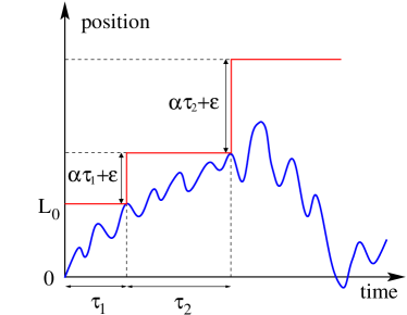
Figure 1: Illustration of the moving boundary (red line) in a semi-infinite geometry due to first-passage resetting. Each time the particle reaches the boundary, the boundary recedes by a distance $\alpha\tau_{i}+\epsilon$. The successive first-passage times are denoted $\tau_{1},\tau_{2},\ldots$.

In this work, we study another natural scenario for first-passage resetting where the boundary recedes by an amount that is proportional to the time difference between successive encounters of the particle and the interface (figure 1). Thus we investigate the dynamics of a one-dimensional Brownian particle with diffusion coefficient $D$ that starts at the origin in a semi-infinite geometry, with a boundary that is initially a distance $L_{0}$ from the particle. This boundary remains fixed except for these instances when the particle reaches it. When such an encounter happens, the boundary moves away from the particle by a distance that is proportional to the first-passage time between the previous and the current encounter. While there is no obvious physical motivation for this model, the resulting phenomenology is quite rich and perhaps has some fundamental implications.

As illustrated in figure 1, it is necessary to augment the recession distance of the interface by a small additive amount to regularize a singular behavior that arises when there is no cutoff. If the interface recedes by an amount that is strictly linear in the first-passage time from the previous collision, a pathology arises in which the particle can hit the interface infinitely often in a finite time. That is, if the first-passage time is short, the time to the next collision can be even shorter, ultimately leading to a singularity. For a random walk on a lattice, there is no such pathology because the minimum first-passage time cannot be less than the time for a single step. To obviate the pathology in the case of continuum diffusion, we define the recession distance of the interface to be equal to the first-passage time from the previous collision plus a small cutoff $\epsilon$. Our results are independent of this cutoff, but this cutoff is necessary to obtain non-singular results.

Our primary results are the following: (a) The probability for the particle to first reach the interface for the $n^{\text{t}h}$ time asymptotically decays as $t^{-\beta_{n}}$, with $\beta_{n}=1+2^{-n}$. Thus the tail of the $n^{\text{th}}$-passage probability becomes progressively fatter after each collision. (b) The number of collisions between the particle and the interface grows with time as $\ln\ln t$. This slow double logarithmic increase in the number of collisions is reminiscent of the intriguing Khintchine iterated logarithm law [16, 17, 18] for the extreme position of Brownian motion. Finally, the position of the interface recedes according to $t/\ln t$. Once again, even though collisions between the particle and the boundary are rare, the widely separated collisions in time lead to a large displacement of the boundary, so that its overall motion is nearly ballistic.

2 Successive-Passage Distributions

2.1 The second-passage distribution

We define $F_{n}(t\,|\,L_{0})$ as the probability that a diffusing particle, which starts at $x=0$, first reaches the boundary at $x=L_{0}$ for the $n^{\text{th}}$ time at time $t$. When $n=1$, this quantity is just the first-passage probability distribution for a Brownian motion to reach $x=L_{0}$ [19, 20]:

$$F_{1}(t\,|\,L_{0})\equiv F(t\,|\,L_{0})=\frac{L_{0}}{\sqrt{4\pi Dt^{3}}}\;e^{-L_{0}^{2}/4Dt}\,.$$ (1)

Because of the convolution structure of the problem we are treating, it is convenient to work in the Laplace domain. Thus we also introduce the Laplace transform of $F_{1}(t\,|\,L_{0})$:

$$\widetilde{F}_{1}(s\,|\,L_{0})=\int_{0}^{\infty}dt\,e^{-st}F_{1}(t\,|\,L_{0})=\,e^{-L_{0}\sqrt{s/D}}\equiv e^{-L_{0}\,g_{1}(s)}\,,$$ (2)

with $g_{1}(s)=\sqrt{s/D}$.

For the particle to first reach the boundary for the second time at time $t$, it must first reach the boundary at an intermediate time $\tau_{1}$ and then reach it one more time during the remaining time $\tau_{2}$, with $t=\tau_{1}+\tau_{2}$. Since the boundary will have moved by a distance $\tau_{1}+\epsilon$ after the first encounter (see figure 1), the second-passage distribution is given by

$$F_{2}(t\,|\,L_{0}) =\int_{0}^{\infty}d\tau_{1}\int_{0}^{\infty}d\tau_{2}\,F_{1}(\tau_{1}\,|\,L_{0})\times F(\tau_{2}\,|\,\alpha\,\tau_{1}+\epsilon)\,\delta(t-\tau_{1}-\tau_{2})\,,$$ (3)

Taking the Laplace transform gives

$$\widetilde{F}_{2}(s\,|\,L_{0}) =\int_{0}^{\infty}d\tau_{1}\int_{0}^{\infty}d\tau_{2}\,F_{1}(\tau_{1}\,|\,L_{0})F(\tau_{2}\,|\,\alpha\,\tau_{1}+\epsilon)\,e^{-s\tau_{1}-s\tau_{2}}\,,$$

$$=\int_{0}^{\infty}d\tau_{1}\,F_{1}(\tau_{1}\,|\,L_{0})\,e^{-s\tau_{1}}\int_{0}^{\infty}d\tau_{2}\,F(\tau_{2}\,|\,\alpha\,\tau_{1}+\epsilon)\,e^{-s\tau_{2}}\,,$$ (4a)

where the second integral is simply the Laplace transform of the first-passage distribution (2) with $$L_{0}=\alpha\tau_{1}+\epsilon$$. Using this fact, we obtain

$$\widetilde{F}_{2}(s\,|\,L_{0}) =\int_{0}^{\infty}d\tau_{1}\,F_{1}(\tau_{1}\,|\,L_{0})\,e^{-s\tau_{1}}\;e^{-(\alpha\,\tau_{1}+\epsilon)\sqrt{s/D}}\,,$$

$$=e^{-\epsilon\sqrt{s/D}}\int_{0}^{\infty}d\tau_{1}\,F_{1}(\tau_{1}\,|\,L_{0})e^{-\tau_{1}\left(s+\alpha\sqrt{s/D}\right)}$$ (4b)

The integral is just the Laplace transform of the first-passage distribution (2), but now evaluated at $$s+\alpha\sqrt{s/D}$$. Thus the second-passage probability is

$$\widetilde{F}_{2}(s\,|\,L_{0})=\exp[-\epsilon\sqrt{s/D}-L_{0}\frac{\sqrt{s+\alpha\sqrt{{s}/{D}}}}{\sqrt{D}}\bigg{]}\equiv e^{-\epsilon\sqrt{s/D}-L_{0}\,g_{2}(s)}\,,$$ (4c)

where

$$g_{2}(s)=\frac{\sqrt{s+\alpha\sqrt{s/D}}}{\sqrt{D}}=\frac{\sqrt{s+\alpha g_{1}(s)}}{\sqrt{D}}\,.$$

This expression for $\widetilde{F}_{2}(s\,|\,L_{0})$ cannot be Laplace inverted analytically; however, in the relevant $s\to 0$ limit, its leading behavior simplifies to

$$\widetilde{F}_{2}(s\,|\,L_{0})\to\exp\left[-L_{0}\,\sqrt{\frac{\alpha}{D}}\left(\frac{s}{D}\right)^{1/4}\right]\,,$$

which can be Laplace inverted. The result of this Laplace inversion is

$$\frac{L_{0}}{96t^{5/4}}\left\{\frac{24}{\Gamma\left(\frac{3}{4}\right)}\;_{0}F_{2}\left(;\frac{1}{2},\frac{3}{4};\frac{L_{0}^{4}}{256{t}}\right)-\sqrt{\frac{288}{\pi}}\frac{L_{0}}{t^{1/4}}\,_{0}F_{2}\left(;\frac{3}{4},\frac{5}{4};\frac{L_{0}^{4}}{256{t}}\right)\right.$$

$$\qquad\qquad\qquad\left.+\frac{3L_{0}^{3}}{t^{1/2}\Gamma\left(\frac{5}{4}\right)}\;_{0}F_{2}\left(;\frac{5}{4},\frac{3}{2};\frac{L_{0}^{4}}{256{t}}\right)-\frac{\sqrt{8}\,L_{0}^{3}}{\pi t^{3/4}}\,_{1}F_{3}\left(1;\frac{5}{4},\frac{3}{2},\frac{7}{4};\frac{L_{0}^{4}}{256{t}}\right)\right\}\,,$$ (5)

where ${}_{p}F_{q}$ is the hypergeometric function. The salient feature of this formidable-looking expression is that the second-passage probability asymptotically decays as $t^{-5/4}$.

2.2 The $n^{\text{th}}$-passage distribution

By repeatedly applying the reasoning that led to (4c), the Laplace transform of the $n^{\text{th}}$-passage probability is

$$\widetilde{F}_{n}(s\,|\,L_{0})=\exp[-\epsilon\sum_{m=1}^{n-1}g_{m}(s)-L_{0}\,g_{n}(s)\bigg{]}\,,$$ (6)

where, for $n\geq 2$, $g_{n}(s)$ is defined by the recursion

$$g_{n}(s)=\frac{\sqrt{s+\alpha\,g_{n-1}(s)}}{\sqrt{D}}\,.$$ (7)

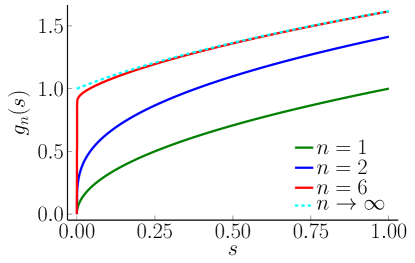
Figure 2: The function $g_{n}(s)$ as a function of $s$ for different values of $n$ with $\alpha=D=1$.

The analytical structure of $g_{n}(s)$ provides the key to understanding the problem. In the limit $n\rightarrow\infty$ and $s$ fixed, $g_{n}(s)\rightarrow g_{\infty}(s)$, where $g_{\infty}(s)$ satisfies $g_{\infty}(s)=\sqrt{(s+\alpha\,g_{\infty}(s))/D}$. The solution for $g_{\infty}(s)$ is

$$g_{\infty}(s)=\frac{1}{2}\left(\frac{\alpha}{D}+\sqrt{\frac{\alpha^{2}}{D^{2}}+\frac{4s}{D}}\right)\,.$$ (8)

The function $g_{n}(s)$ is shown in figure 2 for several values of $n$, as well as for $n=\infty$. Notice that $g_{n}(s)\to 0$ as $s\to 0$ for any finite $n$, while $g_{\infty}(s\!=\!0)=\alpha/D$. Also, when $\alpha=0$, (6) reduces to the $n^{\text{th}}$-resetting probability distribution that we obtained previously [4].

For $s\to 0$ and fixed $n$, the recurrence (7) reduces to

$$g_{n}(s)\sim\left(\frac{\alpha}{D}\right)^{1-2^{1-n}}\;\left(\frac{s}{D}\right)^{2^{-n}}\,.$$ (9)

Thus $g_{n}(s)$ becomes more singular as $n$ increases in such a way that $g_{\infty}(0)=\alpha/D$. We now substitute the above limiting behavior in (6), to give the small-$s$ expansion of the $n^{\text{th}}$ passage distribution:

$$\widetilde{F}_{n}(s\,|\,L_{0})\sim 1-L_{0}\left(\frac{\alpha}{D}\right)^{1-2^{1-n}}\left(\frac{s}{D}\right)^{2^{-n}}\,,\qquad s\rightarrow 0\,.$$ (10a)

By a Tauberian theorem (for a simple derivation see Appendix A.2 of [21]), this gives the power-law decay in the time domain

$$F_{n}(t\,|\,L_{0}) \sim\frac{L_{0}\,\alpha^{1-2^{1-n}}}{-\Gamma(-2^{-n})D^{1-2^{-n}}}\,\frac{1}{t^{1+2^{-n}}}\,,\qquad t\rightarrow\infty\,.$$ (10b)

Thus the long-time tail of the $n^{\text{th}}$-passage probability decays progressively more slowly as $n$ increases, with the exponent value approaching $-1$ for $n\to\infty$.

3 Number of Encounters with the Boundary

Because the tail of the $n^{\text{th}}$-passage probability becomes fatter as $n$ increases, the times between encounters also become progressively longer. Thus we might expect that the total number of encounters will increase only quite slowly with time. We now show that this naive expectation is what actually occurs. Let $N(t)$ denote the number of times that the particle reaches the boundary at time $t$. The probability that there are exactly $n$ encounters at time $t$ is formally given by

$$P(N(t)\!=\!n\,|\,L_{0}) =P(N(t)\!\geq\!n\,|\,L_{0})-P(N(t)\!\geq\!n+1\,|\,L_{0})\,,$$

$$=\int_{0}^{t}d\tau F_{n}(\tau\,|\,L_{0})-\int_{0}^{t}d\tau F_{n+1}(\tau\,|\,L_{0})\,.$$ (11)

The average number of encounters $\langle N(t)\rangle$ is given by

$$\langle N(t)\rangle=\sum_{n=0}^{\infty}n\,P(N(t)\!=\!n\,|\,L_{0})\,.$$ (12a)

We substitute in $$P(N(t)\!=\!n\,|\,L_{0}) n=0$$ from Eq. (3), exploit the telescopic nature of the sum, and also note that the gives no contribution, to obtain

$$\langle N(t)\rangle=\sum_{n=1}^{\infty}P(N(t)\!\geq\!n\,|\,L_{0})=\sum_{n=1}^{\infty}\int_{0}^{t}d\tau F_{n}(\tau\,|\,L_{0})\,.$$ (12b)

In the Laplace domain, the above relation becomes

$$\langle\widetilde{N}(s)\rangle=\frac{1}{s}\sum_{n=1}^{\infty}\widetilde{F}_{n}(s\,|\,L_{0})\,.$$ (13a)

We now substitute the expression (6) for the Laplace transform of the $$n^{\text{th}}$$-passage probability and find that the Laplace transform of the average number of encounters is

$$\langle\widetilde{N}(s)\rangle=\frac{1}{s}\sum_{n=1}^{\infty}\exp\left[-\epsilon\sum_{m=1}^{n-1}g_{m}(s)-L_{0}\,g_{n}(s)\right]\,,$$ (13b)

with $$g_{n}(s)$$ given in (7).

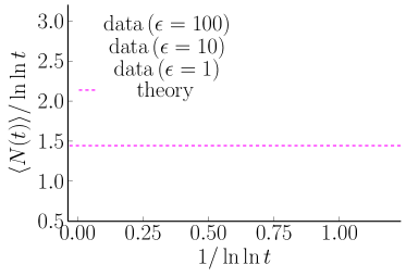
Figure 3: Average number of boundary encounters $\langle N(t)\rangle$ scaled by $\ln\ln t$ as a function of the inverse of the scaled time for $D=L=\alpha=1$. The theoretical prediction from (14b) is also shown.

To obtain the long-time asymptotics, we focus on the $s\to 0$ limit of the above expression:

$$\langle\widetilde{N}(s)\rangle\sim\frac{1}{s}\sum_{n=1}^{\infty}\exp\left[-\epsilon\sum_{m=1}^{n-1}\frac{\alpha^{1-2^{1-m}}}{D^{1-2^{-m}}}\,s^{2^{-m}}-L_{0}\frac{\alpha^{1-2^{1-n}}}{D^{1-2^{-n}}}\,s^{2^{-n}}\right]\,.$$ (13c)

As shown in A, this limiting behavior of $\langle\widetilde{N}(s)\rangle$ reduces to

$$\langle\widetilde{N}(s)\rangle\sim\frac{1}{s\ln 2}\;\ln\left[\ln(\frac{1}{s})\right]\,,$$ (14a)

which, in the time domain, gives the long-time behavior

$$\langle N(t)\rangle\sim\frac{1}{\ln 2}\ln\ln t\approx 1.4427\,\ln\ln t\,.$$ (14b)

This dependence agrees well with numerical simulations for the number of encounters shown in figure 3.

4 Location of the Boundary

We now study the time dependence of the location of the boundary. Let $P(L,t)$ denote the spatial location of the boundary at time $t$. This probability distribution is given by

$$P(L,t) =\delta(L-L_{0})\;\text{erf}\left(\frac{L_{0}}{\sqrt{4\pi Dt}}\right)$$

$$+\sum_{n=1}^{\infty}\int_{0}^{\infty}\!\!d\tau_{1}\ldots d\tau_{n}\,F_{1}(\tau_{1}\,|\,L_{0})\times\ldots\times F(\tau_{n}\,|\,\alpha\,\tau_{n-1}\!+\!\epsilon)\,\delta(L\!-\!L_{0}\!-\!n\epsilon\!-\!\sum_{m=1}^{n}\alpha\tau_{m})$$

$$\quad\times\text{erf}\left(\frac{\alpha\tau_{n}+\epsilon}{\sqrt{4\pi D(t-\sum_{m=1}^{n}\tau_{m})}}\right)\Theta(t-\alpha\sum_{m=1}^{n}\tau_{m})\,.$$ (15)

The first term accounts for the case where the diffusing particle never reaches the boundary. The $n^{\text{th}}$ term in the sum accounts for the case where the particle reaches the boundary $n$ times. Thus there must be a first passage, a second passage,…, up to an $n^{\text{th}}$ passage, after which the particle cannot reach the boundary again. These events are accounted for by the product of $n$ first-passage probabilities and the trailing error function. The theta function imposes the condition that the total time must be larger than the sum of the previous $n$ hitting times. To simplify notation in the formulas below, we introduce $T_{n}\equiv\sum_{m=1}^{n}\tau_{m}$, the sum of the first $n$ time intervals between successive encounters.

Computing the average value gives

$$\langle L(t)\rangle =L_{0}\,\text{erf}\left(\frac{L_{0}}{\sqrt{4\pi Dt}}\right)$$

$$+\sum_{n=1}^{\infty}\int_{0}^{\infty}d\tau_{1}\ldots d\tau_{n}\,F(\tau_{1}\,|\,L_{0})\times\ldots\times F(\tau_{n}\,|\,\alpha\,\tau_{n-1}\!+\!\epsilon)\,(L_{0}\!+\!n\epsilon\!+\!\alpha T_{n})$$

$$\quad\times\text{erf}\left(\frac{\alpha\tau_{n}+\epsilon}{\sqrt{4\pi D(t-T_{n})}}\right)\Theta(t-T_{n})\,.$$ (16)

It is now useful to Laplace transform the above relation. This gives

$$\langle\widetilde{L}(s)\rangle =\frac{L_{0}}{s}\,\left(1-e^{-L_{0}\sqrt{\frac{s}{D}}}\right)$$

$$+\frac{1}{s}\sum_{n=1}^{\infty}\int_{0}^{\infty}d\tau_{1}\ldots d\tau_{n}\,F(\tau_{1}\,|\,L_{0})\times\ldots\times F(\tau_{n}\,|\,\alpha\,\tau_{n-1}+\epsilon)\,(L_{0}+n\epsilon+\alpha T_{n})$$

$$\quad\times\left(1-e^{-(\alpha\tau_{n}+\epsilon)\sqrt{{s}/{D}}}\right)e^{-sT_{n}}\,.$$ (17a)

We argue that the main contribution to $$\langle\widetilde{L}(s)\rangle n \tau_{n}$$ comes from the large- terms in the sum. These terms will involve values of that typically are also large. Thus it is plausible that the exponential term in the parentheses in the last line is negligible. With this assumption, we find

$$\langle\widetilde{L}(s)\rangle \sim\frac{1}{s}\sum_{n=1}^{\infty}\int_{0}^{\infty}\!\!d\tau_{1}\ldots d\tau_{n}\,F(\tau_{1}\,|\,L_{0})\times\ldots\times F(\tau_{n}\,|\,\alpha\,\tau_{n-1}+\epsilon)\,(L_{0}\!+\!n\epsilon\!+\!\alpha T_{n})e^{-sT_{n}}\,,$$ (17b)

where we also drop the first term because it is negligible. Furthermore, the integral of the $n$-fold product of first-passage probabilities is simply $\widetilde{F}_{n}(s\,|\,L_{0})$. Using this identification, we can write the average in the simpler form

$$\langle\widetilde{L}(s)\rangle \sim\frac{1}{s}\left[\sum_{n=1}^{\infty}\left(L_{0}+n\epsilon-\alpha\,\frac{\partial}{\partial s}\right)\widetilde{F}_{n}(s\,|\,L_{0})\right]\,.$$ (18)

Following similar reasoning as that given in A, the leading-order behavior is given by the last term in the brackets. Thus

$$\langle\widetilde{L}(s)\rangle\sim-\frac{\alpha}{s}\frac{\partial}{\partial s}\sum_{n=1}^{\infty}\widetilde{F}_{n}(s\,|\,L_{0}) \sim-\frac{\alpha}{s\ln 2}\frac{\partial}{\partial s}\ln\left[\ln\left(\frac{1}{s}\right)\right]\,,$$

$$\sim\frac{\alpha}{s^{2}\ln 2\ln(1/s)}\,,\qquad s\to 0\,.$$ (19a)

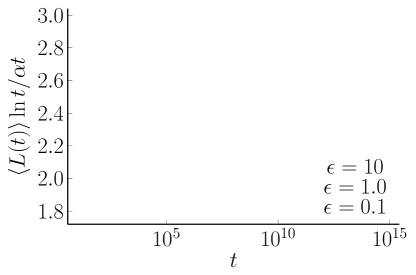
Figure 4: Rescaled average position of the boundary $\langle L(t)\rangle$ as a function of time for $D=L=\alpha=1$.

In the time domain, we then obtain

$$\langle L(t)\rangle\sim\frac{\alpha\,t}{\ln 2\ln t}\,,\qquad t\to\infty\,.$$ (19b)

This asymptotic behavior is in good agreement with numerical simulations as shown in figure 4. The numerical results clearly illustrate that $\langle L(t)\rangle\propto t/\ln(t)$ for $t\to\infty$. However, the amplitude that is found numerically is roughly twice the value of the amplitude that is given in Eq. (19b). We do not know the source of the discrepancy, but it could stem from the neglect of the exponential term in Eq. (17).

5 Concluding Comments

We investigated a simple one-dimensional moving boundary problem that is driven by the motion of a single Brownian particle. This particle moves freely on the infinite line and whenever it encounters the boundary, the boundary instantaneously moves a distance that is proportional to the time between successive collisions between the particle and the boundary. We determined some natural observables of this process. The probability that the particle first hits the boundary for the $n^{\text{th}}$ time asymptotically decays as $t^{-(1+2^{-n})}$. Thus each successive first-passage event is governed by a progressively fatter tail. The number of collisions between the particle and the boundary scales as $\ln\ln t$; this is the same dependence of the iterated logarithm law of free Brownian motion [16, 17, 18], and perhaps there is some unifying mechanism that links our moving boundary problem with free diffusion. In spite of the fact that encounters between the particle and the boundary are rare, the position $L(t)$ of the boundary moves nearly ballistically: $L(t)\sim t/\ln t$. This rapid boundary motion indicates that there must be some long time intervals between successive particle-boundary encounters, so that the boundary moves by a large distance when such an encounter occurs.

Appendix A Asymptotic analysis of $\langle\widetilde{N}(s)\rangle$

In this appendix, we study the small $s$ asymptotic behavior of (13c):

$$\langle\widetilde{N}(s)\rangle\sim\frac{1}{s}\sum_{n=1}^{\infty}\exp\left[-\epsilon\sum_{m=1}^{n-1}\frac{\alpha^{1-2^{1-m}}}{D^{1-2^{-m}}}\;s^{2^{-m}}-L_{0}\frac{\alpha^{1-2^{1-n}}}{D^{1-2^{-n}}}\;s^{2^{-n}}\right]\,,\quad s\to 0\,.$$ (20)

The sum over $n$ can be split roughly into two parts: (i) one is the contribution when $n$ runs from $0$ to $n^{*}=n^{*}(s)$ such that $s^{2^{-n^{*}}}=O(1)$, and (ii) the contribution when $n$ runs from $n^{*}$ to $\infty$. That is

$$\langle\widetilde{N}(s)\rangle\sim\frac{1}{s}\sum_{n=1}^{n^{*}}\exp\left[-L_{0}\frac{\alpha^{1-2^{1-n}}}{D^{1-2^{-n}}}\;s^{2^{-n}}\right]+\frac{1}{s}\sum_{n^{*}}^{\infty}\exp\left[-\epsilon\left(\sum_{m=1}^{n-1}\frac{\alpha^{1-2^{1-m}}}{D^{1-2^{-m}}}\right)-L_{0}\frac{\alpha^{1-2^{1-n}}}{D^{1-2^{-n}}}\right]\,,\quad s\to 0\,.$$ (21)

Because the series in the second term converges, we are left with

$$\langle\widetilde{N}(s)\rangle\sim\frac{1}{s}\sum_{n=1}^{n^{*}}\exp\left[-L_{0}\frac{\alpha^{1-2^{1-n}}}{D^{1-2^{-n}}}\,s^{2^{-n}}\right]\,,\qquad s\to 0\,.$$ (22)

Because the second term is negligible, the final result is independent of the cutoff $\epsilon$. The terms for $n<n^{*}$ will tend to $1$, and therefore we find

$$\langle\widetilde{N}(s)\rangle\sim\frac{1}{s}\,n^{*}\,,\quad s\to 0\,.$$ (23)

Finally, using that $s^{2^{-n^{*}}}=O(1)$, we obtain (14a).

References

- [1] Crank J and Crank J 1984 Free and moving boundary problems (Oxford University Press, USA)
- [2] Rubinstein L 2000 The Stefan Problem vol 8 (American Mathematical Society)
- [3] Langer J S 1980 Rev. Mod. Phys. 52(1) 1–28 URL https://link.aps.org/doi/10.1103/RevModPhys.52.1
- [4] De Bruyne B, Randon-Furling J and Redner S 2021 Journal of Statistical Mechanics: Theory and Experiment 2021 013203
- [5] Evans M R and Majumdar S N 2011 Phys. Rev. Lett. 106 160601
- [6] Evans M R and Majumdar S N 2011 J. Phys. A: Mathematical and Theoretical 44 435001
- [7] Evans M R, Majumdar S N and Schehr G 2020 J. Phys. A: Mathematical and Theoretical
- [8] Boyer D and Solis-Salas C 2014 Phys. Rev. Lett. 112(24) 240601
- [9] Christou C and Schadschneider A 2015 J. Phys. A: Mathematical and Theoretical 48 285003
- [10] Rotbart T, Reuveni S and Urbakh M 2015 Phys. Rev. E 92(6) 060101
- [11] Majumdar S N, Sabhapandit S and Schehr G 2015 Phys. Rev. E 92(5) 052126
- [12] Reuveni S 2016 Phys. Rev. Lett. 116 170601
- [13] Pal A and Reuveni S 2017 Phys. Rev. Lett. 118 030603
- [14] Belan S 2018 Phys. Rev. Lett. 120 080601
- [15] Bodrova A S, Chechkin A V and Sokolov I M 2019 Phys. Rev. E 100 012119
- [16] Khintchine A 1924 Math 32 203–219
- [17] Feller W 2008 An Introduction to Probability Theory and its Applications (John Wiley & Sons)
- [18] Mörters P and Peres Y 2010 Brownian motion vol 30 (Cambridge University Press)
- [19] Redner S 2001 A Guide to First-Passage Processes (Cambridge University Press)
- [20] Bray A J, Majumdar S N and Schehr G 2013 Advances in Physics 62 225–361
- [21] Evans M, Majumdar S N and Zia R 2006 Journal of Statistical Physics 123 357–390