Random coordinate descent methods for nonseparable composite optimization

Abstract

In this paper we consider large-scale composite optimization problems having the objective function formed as a sum of two terms (possibly nonconvex), one has (block) coordinate-wise Lipschitz continuous gradient and the other is differentiable but nonseparable. Under these general settings we derive and analyze two new coordinate descent methods. The first algorithm, referred to as coordinate proximal gradient method, considers the composite form of the objective function, while the other algorithm disregards the composite form of the objective and uses the partial gradient of the full objective, yielding a coordinate gradient descent scheme with novel adaptive stepsize rules. We prove that these new stepsize rules make the coordinate gradient scheme a descent method, provided that additional assumptions hold for the second term in the objective function. We present a complete worst-case complexity analysis for these two new methods in both, convex and nonconvex settings, provided that the (block) coordinates are chosen random or cyclic. Preliminary numerical results also confirm the efficiency of our two algorithms on practical problems.

90C25, 90C15, 65K05.

1 Introduction

In this paper we consider solving large-scale composite optimization problems of the form:

(1) $$F^{*}=\min_{x\in\mathbb{R}^{n}}F(x)\quad\left(:=f(x)+\psi(x)\right),\vspace{-0.05cm}$$

where the function $f:\mathbb{R}^{n}\to\mathbb{R}$ has block coordinate-wise Lipschitz gradient and $\psi:\mathbb{R}^{n}\to{\mathbb{R}}$ is twice continously differentiable function (both terms are possibly nonseparable and nonconvex). Optimization problems having this composite structure permit to handle general coupling functions $\psi$ (e.g., $\psi(x)=\|Ax\|^{p}$, with A linear operator and $p\geq 2$) and arise in many applications such as distributed control, signal processing, machine learning, network flow problems and other areas [6, 24, 27]. Despite the bad properties of the sum (nonsmoothness), such problems, both in convex and nonconvex cases, can be solved by full gradient or Newton methods with the efficiency typical for the good (smooth) part of the objective [33]. However, for large-scale problems, the usual methods based on full gradient and Hessian computations are prohibitive. In this case, it appears that a reasonable approach to solve such problems is to use (block) coordinate descent methods.

State of the art. Coordinate (proximal) gradient descent methods [5, 8, 13, 21, 31, 28, 29, 26, 34, 36, 39], see also the recent survey [40], gained attention in optimization in the last years due to their fast convergence and small computational cost per iteration. The main differences in all variants of coordinate descent algorithms consist in the way we define the local approximation function over which we optimize and the criterion of choosing at each iteration the coordinate over which we minimize this local approximation. For updating one (block) variable, while keeping the other variables fixed, two basic choices for the local approximation are usually considered: (i) exact approximation function, leading to coordinate minimization methods [4, 15] and (ii) quadratic approximation function, leading to coordinate gradient descent methods [31, 39, 40]. Furthermore, three criteria for choosing the coordinate search used often in these algorithms are the greedy, the cyclic and the random coordinate search, respectively. For cyclic coordinate search convergence rates have been given recently in [4, 5]. Convergence rates for coordinate descent methods based on the Gauss-Southwell rule were derived in [39]. Another interesting approach is based on random coordinate descent, where the coordinate search is random. Complexity results on random coordinate descent methods were obtained in [31] for smooth convex functions. The extension to composite objective functions were given in [13, 34, 28, 36]. However, these papers studied optimization models where the second term, usually assumed nonsmooth, is separable, i.e., $\psi(x)=\sum_{i=1}^{n}\psi_{i}(x_{i})$, with $x_{i}$ is the $i$th component of $x$. In the sequel, we discuss papers that consider the case $\psi$ nonseparable and explain the main differences with our present work.

Previous work. From our knowledge there exist few studies on coordinate descent methods when the second term in the objective function is nonseparable. For example, [25, 29, 39] considers the composite optimization problem (1) with $\psi$ convex and separable (possibly nonsmooth) and the additional nonseparable constraints $Ax=b$. Hence, nonseparability comes from the linear constraints. In these settings, [25, 29, 39] proposed coordinate proximal gradient descent methods that require solving at each iteration a subproblem over a subspace generated by the matrix $U\in\mathbb{R}^{n\times p}$ using a part of the gradient of $f$ at the current feasible point $x$, $\nabla f(x)$, i.e:

$$\min_{d\in\mathbb{R}^{p}}f(x)+\langle U^{T}\nabla f(x),d\rangle+\frac{1}{2}d^{T}H_{U}d+\psi(x)\quad\text{s.t.}\quad AUd=0,\vspace*{-0.2cm}$$

where $H_{U}$ is an appropriate positive definite matrix and then update $x^{+}=x+Ud$. The matrix $U$ is chosen according to some greedy rule or random. For these algorithms sublinear rates are derived in the (non)convex case and linear convergence is obtained for strongly convex objective. Further, for problem (1), with $\psi$ possibly nonseparable and nonsmooth, [16, 17, 19] consider proximal coordinate descent methods of the form:

(2) $$\bar{x}^{+}\in\text{prox}_{\alpha\psi}(\mathcal{C}(x-\alpha\nabla f(x))),\vspace*{-0.2cm}$$

where $\mathcal{C}(\cdot)$ is a correction map corresponding to the chosen random subspace at the current iteration in [16, 17] and is the identity map in [19]. Moreover, [16, 17] assume $\psi$ convex and update $x^{+}=\bar{x}^{+}$, while in [19] $\psi$ is possibly nonconvex and updates $x_{i}^{+}=\bar{x}_{i}$ for all $i\in\mathcal{I}\subseteq[n]$ and keeps the rest of the components unchanged. Note that [16, 17] use only a sketch of the gradient $\nabla f(x)$ on the selected subspace, while in [19] $f$ is assumed separable. Since in these papers [16, 17, 19], one needs to compute at each iteration a block of components of the full prox of the nonseparable function $\psi$, $\text{prox}_{\alpha\psi}$, this can be can done efficiently when this prox can be evaluated easily based on the previously computed prox and providec that only a block of coordinates are modified in the prior iteration. For the algorithms in [16, 17] linear convergence is derived, provided that the objective function is strongly convex. Linear convergence results were also obtained in [19] when the objective function satisfies the Kurdyka-Lojasiewicz condition. Recently, [1] considers problem (1), where the function $f$ is assumed quadratic and convex, while $\psi$ convex function (possibly nonseparable and nonsmooth). Under these settings, [1] combines the forward-backward envelope (to smooth the original problem) with an accelerated coordinate gradient descent method and derives sublinear rates for the proposed scheme. This method also makes sense when the full prox can be computed efficiently under coordinate descent updates. The main difference between our work and [16, 17, 19, 1] is that in our first algorithm we consider a prox along coordinates, while in the other papers one needs to compute a block of components of the full prox. Moreover, in the second algorithm our search direction is based on the partial gradient of the full objective function.

The paper most related to the first algorithm is [26]. More precisely, in [26] at each iteration one needs to sketch the gradient $\nabla f$ and compute the prox of $\psi$ along some subspace generated by the random matrix $U\in\mathbb{R}^{n\times p}$, that is:

(3) $$x^{+}=\text{prox}_{H_{f,U}^{-1}\phi}\left(-H_{f,U}^{-1}\;U^{T}\nabla f(x)\right),\vspace*{-0.2cm}$$

where $\phi(d)=\psi(x+Ud)$. Assuming that $\psi$ is twice differentiable, (sub)linear convergence rates are derived in [26] for both convex and nonconvex settings. However, depending on the properties of the random matrix $U$, in each iteration we need to update a block of components of $x$, whose dimension $p$, in some cases, may depend on $n$. In this paper we also design for the composite problem (1) a random coordinate proximal gradient method of the form (3) that uses a block of components of the gradient $\nabla f$ and requires the computation of the prox of $\psi$ along these coordinates. However, in this algorithm we do not have restrictions on the subspace dimension, in the extreme case we can update only one component of $x$. In this paper, we also propose a second algorithm, which contrary to the usual approach from literature, disregards the composite form of the objective function and makes an update based on the partial gradient of the full objective function:

(4) $$x^{+}=x-H_{F,U}^{-1}U^{T}\nabla F(x).\vspace*{-0.1cm}$$

We propose several new adaptive stepsize rules, $H_{F,U}$, based on some additional assumptions on the second term $\psi$.

Contributions. This paper deals with large-scale composite optimization problems of the form (1). We present two coordinate descent methods, (3) and (4), and derive convergence rates when the (block) coordinates are chosen random or cyclic. More precisely, our contributions are:
(i) We introduce a coordinate proximal gradient method, (3), which takes into account the nonseparable composite form of the objective function. In each iteration, one needs to compute a block of components of the gradient $\nabla f$, followed by the prox of $\psi$ along this block of coordinates. Note that typically, the prox restricted to some subspace leads to much less computations than the full prox.
(ii) We also present a coordinate gradient method, (4), which requires at each iteration the computation of a block of components of the gradient of the full objective function, i.e., $U^{T}\nabla F$. We propose new stepsizes strategies for this method, which guarantees descent and convergence under certain assumptions on $\psi$. In particular, three of these stepsize rules are adaptive and require computation of a positive root of a polynomial, while the last one can be chosen constant.
(iii) We derive sufficient conditions for the iterates of our algorithms to be bounded. We also prove that our algorithms are descent methods and derive sublinear convergence rates, provided that the (block) coordinates are chosen random or cyclic, in the convex and nonconvex settings. Improved rates are given under Kurdyka-Lojasiewicz (KL) property, i.e., sublinear or linear depending on the KL parameter. The convergence rates obtained in this paper are summarized in Table 1. Since uniform convex functions satisfy KL property, our rates also cover this case.

Note that in this paper we perform a full convergence analysis for a random coordinate descent algorithm for solving general (non)convex composite problems and most of our variants of coordinate descent schemes were never explicitly considered in the literature before. Although our algorithms belong to the class of coordinate gradient descent methods, our convergence results are also of interest when $f\equiv 0$ and $\psi$ nonseparable (in this case our first algorithm can be viewed as a proximal regularization of a multi-block Gauss-Seidel method). In particular, this is the first work where convergence bounds are presented for an exact coordinate minimization (Gauss-Seidel) method, i.e., when $f\equiv 0$, and for a coordinate gradient descent method, i.e., when the full function $F$ doesn’t have coordinate-wise Lipschitz gradient, in both convex and nonconvex settings. Recall that if $\psi$ is nonseparable, coordinate descent methods may not converge (see e.g., the counterexamples in [14] for nonseparable nondifferentiable convex problems and in [6, 35] for nonseparable nonconvex problems, even in the differentiable case). These results motivate us to consider $\psi$ twice differentiable.

Random
Nonconvex	$\min\limits_{i=0:k-1}\!\mathbb{E}\left[\|\nabla F(x_{i})\|\right]\!\leq\!\mathcal{O}\!\left(\!Nk^{-\frac{1}{2}}\!\right)$	Rem. 6.3	$\forall\delta>0$, with prob. $1-\delta$: $\mathbb{E}\left[F(x_{k})\right]\to F_{*}$ sublinearly or linearly	Thm. 6.8
Convex	$\displaystyle\mathbb{E}\left[F(x_{k})\right]-F^{*}\!\leq\!\mathcal{O}\left(Nk^{-1}\right)$	Thm. 7.1
Cyclic
Nonconvex	$\min\limits_{i=0:k-1}\!\|\nabla F(x_{i})\|\!\leq\!\mathcal{O}\!\left(\!N^{2}k^{-\frac{1}{2}}\!\right)$	Rem. 6.4	$F(x_{kN})\to F_{*}$ sublinearly, linearly or superlinearly	Thm. 6.13
Convex	$\displaystyle F(x_{kN})-F^{*}\!\leq\!\mathcal{O}\left(Nk^{-1}\right)$	Thm. 7.5

Table 1: Convergence rates derived in this paper for the algorithms (3) and (4).

Content. The paper is organized as follows. In Section 2 we present some preliminary results. We derive in Section 3 the coordinate proximal gradient algorithm, while in Section 4 the coordinate gradient algorithm. In Section 5 we present sufficient conditions for the iterates of our algorithms to be bounded. The convergence rates in the random and cyclic cases are derived in Section 6 for the nonconvex case and in Section 7 for the convex case. Finally, in Section 8 we provide detailed numerical simulations.

2 Preliminaries

In this section we present some definitions, some preliminary results and our basic assumptions for the composite problem (1).

2.1 Assumptions/setup

We consider the following problem settings. Let $U\in\mathbb{R}^{n\times n}$ be a column permutation of the identity matrix $I_{n}$ and further let $U=[U_{1},...,U_{N}]$ be a decomposition of $U$ into $N$ submatrices, with $U_{i}\in\mathbb{R}^{n\times n_{i}}$ and $\sum_{i=1}^{N}n_{i}=n$. Hence, any $x\in\mathbb{R}^{n}$ can be written as $x=\sum_{i=1}^{N}U_{i}x^{(i)}$, where $x^{(i)}=U_{i}^{T}x\in\mathbb{R}^{n_{i}}$. Throughout the paper the following assumptions hold:

Assumption .

For composite optimization problem (1) the following hold:
A.1: Gradient of $f$ is block coordinate-wise Lipschitz continuous with constants $L_{i}$:

(5) $$\|U_{i}^{T}(\nabla f(x+U_{i}h)-\nabla f(x))\|\leq L_{i}\|h\|\quad\forall h\in\mathbb{R}^{n_{i}},x\in\mathbb{R}^{n},i=1:N.$$

A.2: $\psi$ is twice continuously differentiable (possibly nonseparable and nonconvex).
A.3: A solution exists for (1) (hence, the optimal value $F^{*}>-\infty$).

If Assumption 2.1[A1] holds, then we have the relation [31]:

(6) $$|f(x+U_{i}h)-f(x)-\langle U_{i}^{T}\nabla f(x),h\rangle|\leq\frac{L_{i}}{2}\|h\|^{2}\quad\forall h\in\mathbb{R}^{n_{i}},\quad i=1,\cdots,N.\vspace*{-0.1cm}$$

The basic idea of our algorithms consist of choosing $i\in\{1,...,N\}$ uniformly at random or cyclic and update $x\in\mathbb{R}^{n}$ as follows: $x^{+}=x+U_{i}d.$ We consider two choices for the directions $d$. In Coordinate Proximal Gradient (CPG) algorithm, the direction $d$ is computed by a proximal operator of $\psi$ restricted to the subspace $U_{i}$. In Coordinate Gradient Descent (CGD) algorithm, $d$ is given by a multiple of a block of components of the gradient $\nabla F(x_{k})$.

Definition 2.1.

For any fixed $x\in\mathbb{R}^{n}$ and $i=1:N$ denote $\phi^{x}_{i}:\mathbb{R}^{n_{i}}\to\mathbb{R}$ as:

(7) $$\phi^{x}_{i}(d)=\psi(x+U_{i}d).\vspace*{-0.1cm}$$

We say that the function $\psi:\mathbb{R}^{n}\to\mathbb{R}$ is convex along coordinates if the partial functions $\phi^{x}_{i}:\mathbb{R}^{n_{i}}\to\mathbb{R}$ are convex for all $x\in\mathbb{R}^{n}$ and $i=1:N$.

One can easily notice that there are nonconvex functions $\psi$ which are convex along coordinates. Note that if $\psi$ is twice differentiable, then it is convex along coordinates if $U_{i}^{T}\nabla^{2}\psi(x)U_{i}$ is positive semidefinite matrix for any $x$ and $U_{i}\in\mathbb{R}^{n\times n_{i}}$, with $i=1:N$.

Below, we use the following mean value inequality (see Appendix for a proof).

Lemma 2.2.

Let $G:\mathbb{R}^{n}\to\mathbb{R}^{m}$ be a continuously differentiable function and $J:\mathbb{R}^{n}\to\mathbb{R}^{m\times n}$ be its Jacobian. Consider $U\in\mathbb{R}^{n\times r}$ a fixed matrix and $x,x+Ud\in\mathbb{R}^{n}$, with $d\in\mathbb{R}^{r}$. Then, there exists $y\in[x,x+Ud]$ such that:

$$\|G(x+Ud)-G(x)\|\leq\|J(y)U\|\|d\|.$$

2.2 KL property

Let us recall the definition of the Kurdyka-Lojasiewicz (KL) property for a function, see e.g., [7]. Note that the KL property is defined for general functions (possibly nondifferentiable). Below, we adapt this definition to the differentiable case, since in this paper we consider only differentiable objective functions.

Definition 2.3.

A differentiable function $F$ satisfies KL property on a compact set $\Omega$ on which $F$ takes a constant value $F_{*}$ if there exist $\gamma,\epsilon>0$ such that one has:

$$\kappa^{\prime}(F(x)-F_{*})\|\nabla F(x)\|\geq 1\quad\forall x\!:\text{dist}(x,\Omega)\leq\gamma,\;F_{*}<F(x)<F_{*}+\epsilon,\vspace*{-0.1cm}$$

where $\kappa:[0,\epsilon]\to\mathbb{R}$ is a concave differentiable function satisfying $\kappa(0)=0$ and $\kappa^{\prime}>0$.

The KL property holds for semi-algebraic functions (e.g., real polynomial functions), vector or matrix (semi)norms (e.g., $\|\cdot\|_{p}$ with $p\geq 0$ rational number), logarithm functions, exponential functions and uniformly convex functions, see [7] for a comprehensive list.

3 A coordinate proximal gradient algorithm

In this section we assume that the function $\psi$ is simple, i.e., $\psi$ restricted to any subspace generated by $U_{i}\in\mathbb{R}^{n\times n_{i}}$ is proximal easy. For minimizing the composite problem (1), where $f$ and $\psi$ are possibly nonseparable and nonconvex, we propose a pure coordinate proximal gradient algorithm that requires some block of components of the gradient $\nabla f(x)$ and computes the prox of $\psi$ also along these block of coordinates. Hence, our Coordinate Proximal Gradient (CPG) algorithm is as follows:

Algorithm 1 (CPG): Given a starting point $x_{0}\in\mathbb{R}^{n}$. For $k\geq 0$ do: 1.   Choose $i_{k}\in\{1,...,N\}$ uniformly at random or cyclic and $\eta_{i_{k}}>0$. Set: (8) $$H_{f,U_{i_{k}}}=\left\{\begin{array}[]{ll}\dfrac{L_{i_{k}}+\eta_{i_{k}}}{2}\;\text{ if }\psi\;\text{convex along coordinates}\\ L_{i_{k}}+\eta_{i_{k}}\;\text{ otherwise}\end{array}\right.$$ 2.   Find $d_{k}$ solving the following subproblem: (9) $$\;\;d_{k}\in\arg\min_{d\in\mathbb{R}^{n_{i_{k}}}}f(x_{k})+\langle U^{T}_{i_{k}}\nabla f(x_{k}),d\rangle+\dfrac{H_{f,U_{i_{k}}}}{2}\|d\|^{2}+\psi(x_{k}+U_{i_{k}}d)\vspace*{-0.1cm}$$ 3.   Update $x_{k+1}=x_{k}+U_{i_{k}}d_{k}$.

Note that for $U_{i_{k}}=I_{n}$, CPG recovers the full proximal gradient method, algorithm (46) in [32], while for $f\equiv 0$ we get a Gauss-Seidel type algorithm similar to [15]. However, [32] derives rates only in the convex settings, while there are very few results ensuring that the iterates of a Gauss-Seidel method converges to a global minimizer, even for strictly convex functions, e.g., [15] presents only assymptotic convergence results. In this paper we derive convergence rates for the general algorithm CPG in both convex and nonconvex settings. An important fact concerning our approach is that the convergence of CPG works for any $\eta_{i_{k}}$ greater than a fixed positive parameter which can be chosen arbitrarily small. In particular, in CPG we can choose a larger stepsize when $\psi$ is convex along coordinates (see Definition 2.1), since $H_{f,U_{i_{k}}}$ must satisfy in this case $H_{f,U_{i_{k}}}>L_{i_{k}}/2$. When $\psi$ is $\rho$-weakly convex along coordinates, the subproblem (9) is convex, provided that $H_{f,U_{i}}\geq\rho$. Our algorithm requires computation of the proximal operator only of the partial function $\phi_{i_{k}}^{x_{k}}$ (defined in (7)) at $U^{T}_{i_{k}}\nabla f(x_{k})$:

(10) $$d_{k}\in\text{prox}_{H_{f,U_{i_{k}}}^{-1}\phi_{i_{k}}^{x_{k}}}\left(-H_{f,U_{i_{k}}}^{-1}\;U^{T}_{i_{k}}\nabla f(x_{k})\right).\vspace*{-0.1cm}$$

Regardless of the properties of the two functions $f$ and $\psi$, the subproblem (9) in CPG is convex provided that $\psi$ is (weakly) convex along coordinates and then the prox operator (10) is well-defined (and unique) in this case, while for general nonconvex $\psi$, the prox (10) has to be interpreted as a point-to-set mapping. The proximal mapping is available in closed form for many useful functions, e.g., for norm power $p$ regularizers. Note that the prox restricted to some subspace (as required in CPG) is much less expensive computationally than the full prox (as required in the literature [16, 17, 19, 32]). More precisely, if $\psi$ is differentiable, then solving the subproblem e.g., in the full proximal gradient method (algorithm (46) in [32]), is equivalent to finding a full vector $d_{k}\in\mathbb{R}^{n}$ satisfying the system of $n$ nonlinear equations:

(11) $$\nabla f(x_{k})+\nabla\psi(x_{k}+d_{k})+H_{f}d_{k}=0.\vspace*{-0.1cm}$$

On other hand, when $N=n$ and $U_{i}=e_{i}$, where $e_{i}$ is the $i$th vector of the canonical basis of $\mathbb{R}^{n}$, at each iteration of our algorithm CPG, solving the subproblem (9) is equivalent to finding a scalar $d_{k}\in\mathbb{R}$ satisfying the scalar nonlinear equation:

(12) $$e^{T}_{i_{k}}(\nabla f(x_{k})+\nabla\psi(x_{k}+d_{k}e_{i_{k}}))+H_{f,U_{i_{k}}}d_{k}=0.\vspace*{-0.1cm}$$

Clearly, there are very efficient methods for finding the root of a scalar equation (12), while it can be more difficult to solve the system of nonlinear equations (11).

Next, we prove that algorithm CPG is a descent method provided that the smooth function $f$ is nonconvex and nonseparable, and $\psi$ is simple, but possibly nonseparable, nonconvex and twice differentiable. Let us denote:

(13) $$\eta_{\min}=\min_{i_{k}=1:N}\eta_{i_{k}}\quad\text{and}\quad H_{f,\max}=\max_{i_{k}=1:N}H_{f,U_{i_{k}}}.$$

Lemma 3.1.

If Assumption 2.1 holds, then iterates of CPG satisfy the descent:

(14) $$F(x_{k+1})\leq F(x_{k})-\dfrac{\eta_{\min}}{2}\|d_{k}\|^{2}\quad\forall k\geq 0.$$

Proof 3.2.

Using Assumption 2.1 and inequality (6), we obtain:

(15) $$f(x_{k+1})+\psi(x_{k+1})\leq f(x_{k})+\langle\nabla f(x_{k}),U_{i_{k}}d_{k}\rangle+\frac{L_{i_{k}}}{2}\|d_{k}\|^{2}+\psi(x_{k+1}).$$

First, consider $\psi$ convex along coordinates. From optimality condition for (9):

$$\langle U^{T}_{i_{k}}\nabla f(x_{k})+H_{f,U_{i_{k}}}d_{k},d-d_{k}\rangle+\psi(x_{k}+U_{i_{k}}d)\geq\psi(x_{k}+U_{i_{k}}d_{k})\quad\forall d\in\mathbb{R}^{n_{i}}.$$

Combining the inequality above for $d=0$ with (15), using (8) and (13), we get:

$$F(x_{k+1}) \leq F(x_{k})+\langle\nabla f(x_{k}),U_{i_{k}}d_{k}\rangle+\frac{L_{i_{k}}}{2}\|d_{k}\|^{2}-\langle U^{T}_{i_{k}}\nabla f(x_{k}),d_{k}\rangle-H_{f,U_{i_{k}}}\|d_{k}\|^{2}$$

(16) $$=F(x_{k})-\left(H_{f,U_{i_{k}}}-\dfrac{L_{i_{k}}}{2}\right)\|d_{k}\|^{2}\leq F(x_{k})-\dfrac{\eta_{\min}}{2}\|d_{k}\|^{2}.$$

Second, consider $\psi$ general function. Since $d_{k}$ is the optimal solution for (9), choosing $d=0$, we have:

(17) $$\langle U^{T}_{i_{k}}\nabla f(x_{k}),d_{k}\rangle+\dfrac{H_{f,U_{i_{k}}}}{2}\|d_{k}\|^{2}+\psi(x_{k}+U_{i_{k}}d_{k})\leq\psi(x_{k}).$$

From inequalities (15) and (17), using (8) and (13), we also get:

(18) $$F(x_{k+1}) \leq f(x_{k})+\langle\nabla f(x_{k}),U_{i_{k}}d_{k}\rangle+\frac{L_{i_{k}}}{2}\|d_{k}\|^{2}+\psi(x_{k+1}).$$

$$\leq F(x_{k})-\dfrac{1}{2}\left(H_{f,U_{i_{k}}}-L_{i_{k}}\right)\|d_{k}\|^{2}\leq F(x_{k})-\dfrac{\eta_{\min}}{2}\|d_{k}\|^{2}.$$

Note that the previous lemma is valid independently on how the index $i_{k}$ is choosen. Moreover, when $i_{k}$ is choosen uniformly at random the iterates $x_{k}$ are random vectors, the function values $F(x_{k})$ are random variables and $x_{k+1}$ depends on $x_{k}$ and $i_{k}$. In the sequel, we assume that the sequence $(x_{k})_{k\geq 0}$ generated by algorithm CPG is bounded. In Section LABEL:Sec:SufCond we will present sufficient conditions when this holds. Next, we will prove some descent w.r.t. the norm of the gradient. Let us first introduce some notations that will be used in the sequel:

(19) $${\color[rgb]{0,0,0}\bar{\nabla}^{2}\Psi(z_{1},\cdots,z_{n})}=\begin{bmatrix}\nabla_{1}^{2}\psi(z_{1})\\ \vdots\\ \nabla_{n}^{2}\psi(z_{n})\end{bmatrix},\vspace*{-0.2cm}$$

with $\nabla_{i}^{2}\psi(z_{i})$ being the $i$th row of the hessian of $\psi$ at the point $z_{i}\in\mathbb{R}^{n}$,

(20) $$H_{F_{i}}=\max_{z_{1},\cdots,z_{n}\in\overline{\text{conv}}\{(x_{k})_{k\geq 0}\}}\|U_{i}^{T}\bar{\nabla}^{2}\Psi(z_{1},\cdots,z_{n})U_{i}+H_{f,U_{i}}I_{n_{i}\times n_{i}}\|,$$

and $H_{F,\max}=\max_{i=1:N}H_{F_{i}}$. Note that CPG algorithm does not require the knowledge of the coordinate-wise Lipschitz constants of the whole function $F$ (or of the term $\psi$). The constant $H_{F,\max}$ only appears in the convergence rates. In some applications the second term, $\psi$, although differentiable, might have expensive gradient evaluation or the corresponding coordinate-wise Lipschitz constants over a bounded set might be difficult to estimate; on the other hand, if the computation of the prox for the second term $\psi$ along a block of coordinates is easy, then algorithm CPG can be used. One example is the function $\psi(x)=\|Ax\|^{p}$, with $p\geq 2$, which has an expensive gradient evaluation when the dimension of matrix $A$ is very large, since we have to compute a matrix-vector product, and its gradient is Lipschitz on any bounded subset, but the coordinate-wise Lipschitz constants are not easy to estimate. On the other hand, if we update only one coordinate at each iteration, solving the subproblem (9) is equivalent to finding a root of a scalar equation. More examples are given in Section 8. For deterministic CPG (i.e., cyclic coordinate choice), let us also define $L$:

(21) $$\|U_{i}^{T}\left(\nabla f(x)-\nabla f(y)\right)\|\leq L\|x-y\|\quad\forall i=1:N\quad\text{and}\quad x,y\in\mathbb{R}^{n},$$

and the constant

(22) $$\bar{H}_{\psi,\max}=\max_{i=1:N,x\in\overline{\text{conv}}\{(x_{k})_{k\geq 0}\}}\|U^{T}_{i}\nabla^{2}\psi(x)\|.\vspace*{-0.2cm}$$

Since $f$ has coordinate-wise Lipschitz gradient, then there exists $L>0$ satisfying (21), see [31].

Lemma 3.3.

If Assumption 2.1 holds and the sequence $(x_{k})_{k\geq 0}$ generated by algorithm CPG is bounded, then we have the following descents:
i) If $i_{k}$ is choosen uniformly at random, we have:

(23) $$\mathbb{E}[F(x_{k+1})\ |\ x_{k}]\leq F(x_{k})-\dfrac{\eta_{\min}}{2NH_{F,\max}^{2}}\|\nabla F(x_{k})\|^{2}.\vspace*{-0.2cm}$$

ii) If $i_{k}$ is choosen cyclic, we have:

(24) $$F(x_{k+N})\leq F(x_{k})-\dfrac{\eta_{\min}}{4N\bar{H}_{\psi,\max}^{2}+8(N-1)L^{2}+8H_{f,\max}^{2}}\|\nabla F(x_{k})\|^{2}.\vspace*{-0.2cm}$$

Proof 3.4.

i) First, we consider $i_{k}$ choosen uniformly at random. Since $f$, $\psi$ are differentiable, from the optimality condition for $d_{k}$, we get:

(25) $$U^{T}_{i_{k}}(\nabla f(x_{k})+\nabla\psi(x_{k+1}))+H_{f,U_{i_{k}}}d_{k}=0.$$

Moreover, $\nabla F(x_{k})=\nabla f(x_{k})+\nabla\psi(x_{k})$ and

$$\mathbb{E}[\|U^{T}_{i_{k}}\nabla F(x_{k})\|^{2}\ |\ x_{k}]=\dfrac{1}{N}\|\nabla F(x_{k})\|^{2}.$$

Combining the equality above with (25), we get:

$$\dfrac{1}{N}\|\nabla F(x_{k})\|^{2} = \mathbb{E}[\|U^{T}_{i_{k}}(\nabla f(x_{k})+\nabla\psi(x_{k}))\|^{2}\ |\ x_{k}]$$

$$= \mathbb{E}[\|U^{T}_{i_{k}}(\nabla\psi(x_{k})-\nabla\psi(x_{k+1}))-H_{f,U_{i_{k}}}d_{k}\|^{2}\ |\ x_{k}].$$

Now, considering the particular form of the matrix $U_{i_{k}}$, using the mean value theorem and the definition of $H_{F_{i_{k}}}$, we further get:

$$\|U^{T}_{i_{k}}(\nabla\psi(x_{k})\!-\nabla\psi(x_{k+1}))-\!H_{f,U_{i_{k}}}d_{k}\|^{2}\!=\!\sum_{j\in I_{k}}|\nabla_{j}\psi(x_{k})-\!\nabla_{j}\psi(x_{k+1})-\!H_{f,U_{i_{k}}}d_{k,j}|^{2}$$

$$=\sum_{j\in I_{k}}|\nabla_{j}^{2}\psi(z_{k,j})U_{i_{k}}d_{k}+H_{f,U_{i_{k}}}d_{k,j}|^{2}=\|U_{i_{k}}^{T}\bar{\nabla}^{2}\Psi(z_{k,1},\cdots,z_{k,n})U_{i_{k}}d_{k}+H_{f,U_{i_{k}}}d_{k}\|^{2}$$

$$\leq\|U_{i_{k}}^{T}\bar{\nabla}^{2}\Psi(z_{k,1},\cdots,z_{k,n})U_{i_{k}}+H_{f,U_{i_{k}}}I_{n_{i_{k}}}\|^{2}\|d_{k}\|^{2}\leq H_{F_{i_{k}}}^{2}\|d_{k}\|^{2}\leq H_{F,\max}^{2}\|d_{k}\|^{2},$$

where $I_{k}$ is the set of indexes chosen at $k$ and $z_{k,j}\in[x_{k},x_{k+1}]$ for all $j\in I_{k}$. Hence, we get:

(26) $$\|\nabla F(x_{k})\|^{2}\leq NH_{F,\max}^{2}\cdot\mathbb{E}\left[\|d_{k}\|^{2}\ |\ x_{k}\right].$$

Finally, taking the conditional expectation of both sides of the inequality (14) w.r.t. $x_{k}$ and combining it with (26), we get (23).
ii) If $i_{k}$ is chosen cyclic, then, with some abuse of notation, let us consider that at the $k$th iteration the first block of coordinates is updated and at the $(k+i_{k}-1)$th iteration, we update the $i_{k}$th block of coordinates. Hence, using the optimality condition (25), we obtain:

$$\|\nabla F(x_{k})\|^{2}=\sum_{i_{k}=1}^{N}\|U_{i_{k}}^{T}\nabla F(x_{k})\|^{2}=\sum_{i_{k}=1}^{N}\|U_{i_{k}}^{T}\left(\nabla f(x_{k})+\nabla\psi(x_{k})\right)\|^{2}$$

$$=\sum_{i_{k}=1}^{N}\|U_{i_{k}}^{T}\left(\nabla f(x_{k})-\nabla f(x_{k+i_{k}-1})+\nabla\psi(x_{k})-\nabla\psi(x_{k+i_{k}})\right)-H_{f,U_{i_{k}}}d_{k+i_{k}-1}\|^{2}$$

$$\leq\sum_{i_{k}=1}^{N}\left(4\|U_{i_{k}}^{T}\left(\nabla f(x_{k})-\nabla f(x_{k+i_{k}-1})\right)\|^{2}+4H_{f,U_{i_{k}}}\|d_{k+i_{k}-1}\|^{2}\right)$$

$$+\sum_{i_{k}=1}^{N}2\|U_{i_{k}}^{T}\left(\nabla\psi(x_{k})-\nabla\psi(x_{k+i_{k}})\right)\|^{2}.$$

Note that $\|x_{k+N}-x_{k}\|^{2}=\displaystyle\sum_{i_{k}=1}^{N}\|d_{k+i_{k}-1}\|^{2}$. Using (13), (21) and the mean value inequality (see Lemma 2.2) with $z_{i_{k}}\in[x_{k},x_{k+i_{k}}]$, we get:

$$\|\nabla F(x_{k})\|^{2} \leq 4H_{f,\max}^{2}\|x_{k+N}-x_{k}\|^{2}+\sum_{i_{k}=1}^{N}4L^{2}\|x_{k}-x_{k+i_{k}-1}\|^{2}$$

$$+\sum_{i_{k}=1}^{N}2\|U_{i_{k}}^{T}\nabla^{2}\psi(z_{i_{k}})\|^{2}\|x_{k+i_{k}}-x_{k}\|^{2}.$$

Note that, since one block of coordinates is updated at each iteration, we have $\|x_{k+i_{k}}-x_{k}\|\leq\|x_{k+N}-x_{k}\|$ for all $i_{k}=1:N-1$. Hence, from (22), we obtain:

(27) $$\|\nabla F(x_{k})\|^{2}\leq\left(2N\bar{H}_{\psi,\max}^{2}+4H_{f,\max}^{2}+4(N-1)L^{2}\right)\|x_{k+N}-x_{k}\|^{2}.$$

Using $\|x_{k+N}-x_{k}\|^{2}=\displaystyle\sum_{i_{k}=1}^{N}\|d_{k+i_{k}-1}\|^{2}$, from inequality (14), we have:

(28) $$F(x_{k+N})\leq F(x_{k})-\dfrac{\eta_{\min}}{2}\sum_{i_{k}=1}^{N}\|d_{k+i_{k}-1}\|^{2}.\vspace*{-0.2cm}$$

Finally, combining (27) and (28), we obtain (24).

Remark 3.5.

Recall that the convergence analysis in [5] for cyclic coordinate descent contains a term $N\bar{L}^{2}$, with $\bar{L}$ the global Lipschitz constant of the gradient of $f$, and $\psi=0$. Note that our $L$ defined in (21) is usually smaller than $\bar{L}$, hence our estimate is usually better.

4 A coordinate gradient descent algorithm

In this section, we present a Coordinate Gradient Descent (CGD) algorithm for solving problem (1), with $f$ and $\psi$ possibly nonseparable and nonconvex. In each iteration, $d_{k}$ is given by some (block) components of the full gradient $\nabla F(x_{k})$.

Algorithm 2 (CGD): Given a starting point $x_{0}\in\mathbb{R}^{n}$. For $k\geq 0$ do: 1.   Choose $i_{k}\in\{1,...,N\}$ uniformly at random or cyclic and compute $H_{F_{k}}>0$ as defined in one of the following equations: (LABEL:eq:HF1), (LABEL:eq:HF2), (LABEL:eq:HF3) or (LABEL:eq:HF4). 2.   Solve the following subproblem: (29) $$\;\;d_{k}=\arg\min_{d\in\mathbb{R}^{n_{i}}}F(x_{k})+\langle U^{T}_{i_{k}}\nabla F(x_{k}),d\rangle+\dfrac{H_{F_{k}}}{2}\|d\|^{2}.\vspace*{-0.1cm}$$ 3.   Update $x_{k+1}=x_{k}+U_{i_{k}}d_{k}$.

From the optimality conditions for the subproblem (29), we have:

(30) $$d_{k}=-\dfrac{1}{H_{F_{k}}}U^{T}_{i_{k}}\nabla F(x_{k})=-\dfrac{1}{H_{F_{k}}}U^{T}_{i_{k}}\left(\nabla f(x_{k})+\nabla\psi(x_{k})\right).$$

The main difficulty with algorithm CGD is that we need to find an appropriate stepsize $H_{F_{k}}$ which ensures descent, although the full objective function $F$ doesn’t have a coordinate-wise Lipschitz gradient. In the sequel we derive novel stepsize rules which combined with additional properties on $\psi$ yield descent. Let us denote:

(31) $$H_{f,U_{i_{k}}}=\dfrac{L_{i_{k}}+\eta_{i_{k}}}{2}.$$

Consider one of the following additional properties on the function $\psi$.

Assumption 4.1.

Assume either:

A.4: Given function $\psi$, there exist $H_{\psi}>0$ and integer $p\geq 1$ such that:

$$\|U_{i}^{T}\nabla^{2}\psi(y)U_{i}\|\leq H_{\psi}\|y\|^{p}\quad\forall y\in\mathbb{R}^{n},\quad i=1:N.$$

A.5: Hessian of $\psi$ is Lipschitz, i.e., there exists $L_{\psi}>0$ such that:

$$\|\nabla^{2}\psi(y)-\nabla^{2}\psi(x)\|\leq L_{\psi}\|y-x\|\quad\forall x,y\in\mathbb{R}^{n}.$$

A.6: Function $\psi$ is differentiable and concave along coordinates, i.e.:

$$\psi(x+U_{i}d)\leq\psi(x)+\langle U_{i}^{T}\nabla\psi(x),d\rangle\quad\forall d\in\mathbb{R}^{n_{i}},x\in\mathbb{R}^{n},i=1:N.$$

See Section 8 for concrete examples of functions satisfying Assumption 4.1 [A.4-A.5].

For simplicity of the exposition, in Table LABEL:table:stepsizes we present four stepsize rules and the corresponding assumptions on $\psi$ which allows us to prove descent for algorithm CGD. Note that, in order to run algorithm CGD, we need to know $H_{\psi}$ or $L_{\psi}$, respectively, and the third stepsize strategy requires computation of $\nabla^{2}\psi$ only in $x_{0}$.

Table 2: Proposed stepsize rules for the algorithm CGD.

	Stepsize choice	Ass. on $\psi$
	1. Choose $H_{f,U_{i_{k}}}>\dfrac{L_{i_{k}}}{2}$ and compute $\alpha_{k}\geq 0$ as root of second order equation in $\alpha$: (32) $$\dfrac{L_{\psi}}{6}\alpha^{2}+\left(\dfrac{H_{\psi}}{2}\|x_{k}\|^{p}+H_{f,U_{i_{k}}}\right)\alpha-\|U_{i_{k}}^{T}\nabla F(x_{k})\|=0.$$ 2. Define (33) $$H_{F_{k}}=\frac{H_{\psi}}{2}\|x_{k}\|^{p}+\frac{L_{\psi}}{6}\alpha_{k}+H_{f,U_{i_{k}}}.\vspace*{-0.2cm}$$
		A.4
1)		and
		A.5
	1. Choose $H_{f,U_{i_{k}}}>\dfrac{L_{i_{k}}}{2}$ and compute $\alpha_{k}\geq 0$ as root of the following polynomial equation in $\alpha$: (34) $$2^{p-1}H_{\psi}\alpha^{p+1}+(2^{p-1}H_{\psi}\|x_{k}\|^{p}+H_{f,U_{i_{k}}})\alpha=\|U_{i_{k}}^{T}\nabla F(x_{k})\|.$$ 2. Define: (35) $$H_{F_{k}}=2^{p-1}H_{\psi}\|x_{k}\|^{p}+2^{p-1}H_{\psi}\alpha_{k}^{p}+H_{f,U_{i_{k}}}.\vspace*{-0.3cm}$$
2)		A.4
	1.   Choose $H_{f,U_{i_{k}}}>\dfrac{L_{i_{k}}}{2}$ and compute $\alpha_{k}\geq 0$ as root of the second order equation: $\displaystyle\dfrac{L_{\psi}}{6}\alpha^{2}+\left(\dfrac{L_{\psi}}{2}\|x_{k}-x_{0}\|+\dfrac{1}{2}\|\nabla^{2}\psi(x_{0})\|+H_{f,U_{i_{k}}}\right)\alpha$ (36) $\displaystyle=\|U_{i_{k}}^{T}\nabla F(x_{k})\|.$ 2.   Update (37) $$\vspace*{-0.1cm}H_{F_{k}}=\frac{L_{\psi}}{2}\|x_{k}-x_{0}\|+\frac{1}{2}\|\nabla^{2}\psi(x_{0})\|+\frac{L_{\psi}}{6}\alpha_{k}+H_{f,U_{i_{k}}}\vspace*{-0.3cm}$$
3)		A.5
	1.   Choose $H_{f,U_{i_{k}}}>\dfrac{L_{i_{k}}}{2}$ and update (38) $$H_{F_{k}}=H_{f,U_{i_{k}}}.\vspace*{-0.1cm}$$
4)		A.6

Note that, the first three stepsize rules are adaptive and require at each iteration computation of a nonnegative root of some polynomial, while the last one is chosen constant. Moreover, the case 4) covers difference of convex (DC) programming problems and our algorithm CGD is new in this context. One can easily see that all the equations (LABEL:eq:103), (LABEL:eq:100) and (LABEL:eq:105) admit a nonnegative root $\alpha_{k}\geq 0$ and thus $H_{F_{k}}$ is well-defined. Indeed, let us check for the second stepsize choice. Consider:

(39) $$h(\alpha)=2^{p-1}H_{\psi}\alpha^{p+1}+(2^{p-1}H_{\psi}\|x_{k}\|^{p}+H_{f,U_{i_{k}}})\alpha-\|U_{i_{k}}^{T}\nabla F(x_{k})\|\vspace*{-0.1cm}$$

and $w_{k}=\dfrac{1}{H_{f,U_{i_{k}}}}\|U_{i_{k}}^{T}\nabla F(x_{k})\|$. If $\|U_{i_{k}}^{T}\nabla F(x_{k})\|\neq 0$, then we have $h(w_{k})>0$ and $h(0)<0$. Since $h$ is continuous on $[0,w_{k}]$, there exists $\alpha_{k}\in(0,w_{k})$ such that $h(\alpha_{k})=0$. Moreover, since $h^{\prime}(\alpha)>0$ for all $\alpha\in(0,+\infty)$, then $h$ is strictly increasing on $(0,+\infty)$. Hence, there exists exactly one $\alpha_{k}>0$ satisfying (LABEL:eq:100). Otherwise, if $\|U_{i_{k}}^{T}\nabla F(x_{k})\|=0$, we have $\alpha_{k}=0$. One can see that the first three stepsizes satisfy:

(40) $$\|d_{k}\|=\dfrac{1}{H_{F_{k}}}\|U_{i_{k}}^{T}\nabla F(x_{k})\|=\alpha_{k}.\vspace*{-0.1cm}$$

Lemma 4.2.

Let Assumptions 2.1 and 4.1 hold such that $H_{F_{k}}$ is updated according to Table LABEL:table:stepsizes. Then, the iterates of algorithm CGD satisfy the descent:

(41) $$F(x_{k+1})\leq F(x_{k})-\dfrac{\eta_{\min}}{2}\|d_{k}\|^{2}.\vspace*{-0.1cm}$$

Proof 4.3.

Consider first case 1), i.e., conditions A.4 and A.5 of Assumption 4.1 hold. From Assumption 4.1[A.5], we have:

$$\psi(x_{k+1})\leq\psi(x_{k})+\langle\nabla\psi(x_{k}),U_{i_{k}}d_{k}\rangle+\dfrac{1}{2}\langle\nabla^{2}\psi(x_{k})U_{i_{k}}d_{k},U_{i_{k}}d_{k}\rangle+\dfrac{L_{\psi}}{6}\|d_{k}\|^{3}.$$

Combining the previous inequality with (6), we obtain:

$$f(x_{k+1})+\psi(x_{k+1})\leq f(x_{k})+\langle\nabla f(x_{k}),U_{i_{k}}d_{k}\rangle+\frac{L_{i_{k}}}{2}\|d_{k}\|^{2}+\psi(x_{k+1})$$

$$\leq f(x_{k})+\langle U_{i_{k}}^{T}\nabla F(x_{k}),d_{k}\rangle+\frac{L_{i_{k}}}{2}\|d_{k}\|^{2}+\psi(x_{k})+\dfrac{1}{2}\langle U_{i_{k}}^{T}\nabla^{2}\psi(x_{k})U_{i_{k}}d_{k},d_{k}\rangle+\dfrac{L_{\psi}}{6}\|d_{k}\|^{3}.$$

Further, from (30), we have:

(42) $$F(x_{k+1})$$

$$\leq F(x_{k})-H_{F_{k}}\|d_{k}\|^{2}+\frac{L_{i_{k}}}{2}\|d_{k}\|^{2}+\dfrac{1}{2}\langle U_{i_{k}}^{T}\nabla^{2}\psi(x_{k})U_{i_{k}}d_{k},d_{k}\rangle+\dfrac{L_{\psi}}{6}\|d_{k}\|^{3}$$

$$\leq F(x_{k})-H_{F_{k}}\|d_{k}\|^{2}+\frac{L_{i_{k}}}{2}\|d_{k}\|^{2}+\dfrac{1}{2}\|U_{i_{k}}^{T}\nabla^{2}\psi(x_{k})U_{i_{k}}\|\|d_{k}\|^{2}+\dfrac{L_{\psi}}{6}\|d_{k}\|^{3}.$$

From Assumption 4.1[A.4], we obtain:

$$F(x_{k+1})\leq F(x_{k})-H_{F_{k}}\|d_{k}\|^{2}+\frac{L_{i_{k}}}{2}\|d_{k}\|^{2}+\dfrac{H_{\psi}}{2}\|x_{k}\|^{p}\|d_{k}\|^{2}+\dfrac{L_{\psi}}{6}\|d_{k}\|^{3}.\vspace*{-0.1cm}$$

From (LABEL:eq:HF1) and (40), we have $H_{F_{k}}=\frac{L_{\psi}}{6}\|d_{k}\|+\frac{H_{\psi}}{2}\|x_{k}\|^{p}+H_{f,U_{i_{k}}}$. Then, from (31) and (13), we get the descent:

(43) $$F(x_{k+1})\leq F(x_{k})-\left(H_{f,U_{i_{k}}}-\frac{L_{i_{k}}}{2}\right)\|d_{k}\|^{2}\leq F(x_{k})-\frac{\eta_{\min}}{2}\|d_{k}\|^{2}.\vspace*{-0.1cm}$$

Consider now case 2), i.e., A.4 of Assumption 4.1 holds. Since $\psi$ is differentiable, from the mean value theorem there exists $y_{k}\in[x_{k},x_{k}+U_{i_{k}}d_{k}]$ such that $\psi(x_{k+1})-\psi(x_{k})=\langle\nabla\psi(y_{k}),U_{i_{k}}d_{k}\rangle$. Combining the last equality with (6), we obtain:

$$f(x_{k+1})+\psi(x_{k+1}) \leq f(x_{k})+\langle\nabla f(x_{k}),U_{i_{k}}d_{k}\rangle+\frac{L_{i_{k}}}{2}\|d_{k}\|^{2}+\psi(x_{k+1})$$

$$= f(x_{k})+\psi(x_{k})+\langle\nabla\psi(y_{k})+\nabla f(x_{k}),U_{i_{k}}d_{k}\rangle+\frac{L_{i_{k}}}{2}\|d_{k}\|^{2}.\vspace*{-0.1cm}$$

Using (30), we further have:

(44) $$F(x_{k+1})\leq F(x_{k})+\langle U_{i_{k}}^{T}\left(\nabla\psi(y_{k})-\nabla\psi(x_{k})\right),d_{k}\rangle-H_{F_{k}}\|d_{k}\|^{2}+\frac{L_{i_{k}}}{2}\|d_{k}\|^{2}.$$

Since $y_{k}\in[x_{k},x_{k}+U_{i_{k}}d_{k}]$, then $y_{k}=(1-\tau)x_{k}+\tau\left(x_{k}+U_{i_{k}}d_{k}\right)$ for some $\tau\in[0,1]$. Moreover, from Lemma 2.2 there exists $\bar{x}_{k}\in[x_{k},y_{k}]$ such that:

$$\|U^{T}_{i_{k}}(\nabla\psi(y_{k})-\nabla\psi(x_{k}))\|\leq\|U^{T}_{i_{k}}\nabla^{2}\psi(\bar{x}_{k})U_{i_{k}}\|\|\tau d_{k}\|\leq\|U^{T}_{i_{k}}\nabla^{2}\psi(\bar{x}_{k})U_{i_{k}}\|\|d_{k}\|.$$

Note that $\bar{x}_{k}=(1-\mu)x_{k}+\mu y_{k}$ for some $\mu\in[0,1]$. From Assumption 4.1[A.4] and the last inequality, we obtain:

$$\langle U_{i_{k}}^{T}\left(\nabla\psi(y_{k})-\nabla\psi(x_{k})\right),d_{k}\rangle \leq \|U_{i_{k}}^{T}\left(\nabla\psi(y_{k})-\nabla\psi(x_{k})\right)\|\|d_{k}\|$$

$$\leq\|U^{T}_{i_{k}}\nabla^{2}\psi(\bar{x}_{k})U_{i_{k}}\|\|d_{k}\|^{2} \leq H_{\psi}\|(1-\mu)x_{k}+\mu y_{k}\|^{p}\|d_{k}\|^{2}.$$

From convexity of $\|\cdot\|^{p}$, for $p\geq 1$, and the fact that $y_{k}=(1-\tau)x_{k}+\tau\left(x_{k}+U_{i_{k}}d_{k}\right)$ for some $\tau\in[0,1]$, we get:

$$\langle U_{i_{k}}^{T}\left(\nabla\psi(y_{k})-\nabla\psi(x_{k})\right),d_{k}\rangle\leq H_{\psi}\left((1-\mu)\|x_{k}\|^{p}+\mu\|y_{k}\|^{p}\right)\|d_{k}\|^{2}$$

$$=H_{\psi}\left((1-\mu)\|x_{k}\|^{p}+\mu\|(1-\tau)x_{k}+\tau\left(x_{k}+U_{i_{k}}d_{k}\right)\|^{p}\right)\|d_{k}\|^{2}$$

$$\leq H_{\psi}\left((1-\mu)\|x_{k}\|^{p}+\mu(1-\tau)\|x_{k}\|^{p}+\mu\tau\|x_{k}+U_{i_{k}}d_{k}\|^{p}\right)\|d_{k}\|^{2}.$$

Since $\mu,\tau\in[0,1]$ and $\|a+b\|^{p}\leq 2^{p-1}\|a\|^{p}+2^{p-1}\|b\|^{p}$ for $p\geq 1$, we get:

$$\langle U_{i_{k}}^{T}\left(\nabla\psi(y_{k})-\nabla\psi(x_{k})\right),d_{k}\rangle \leq H_{\psi}\left((1+(2^{p-1}-1)\mu\tau)\|x_{k}\|^{p}+2^{p-1}\mu\tau\|d_{k}\|^{p}\right)\|d_{k}\|^{2}$$

$$\leq 2^{p-1}H_{\psi}\|x_{k}\|^{p}\|d_{k}\|^{2}+2^{p-1}H_{\psi}\|d_{k}\|^{p+2}.$$

Combining the inequality above with (44), we obtain:

$$F(x_{k+1})\leq F(x_{k})+2^{p-1}H_{\psi}\|x_{k}\|^{p}\|d_{k}\|^{2}+2^{p-1}H_{\psi}\|d_{k}\|^{p+2}-H_{F_{k}}\|d_{k}\|^{2}+\frac{L_{i_{k}}}{2}\|d_{k}\|^{2}.\vspace*{-0.0cm}$$

From (LABEL:eq:HF2) and (40), we have $H_{F_{k}}=2^{p-1}H_{\psi}\|d_{k}\|^{p}+2^{p-1}H_{\psi}\|x_{k}\|^{p}+H_{f,U_{i_{k}}}$. Hence, from (31) and (13), we get the descent (43).

Consider now case 3), i.e., A.5 of Assumption 4.1 holds. From Assumption 2.1, Assumption 4.1[A.5] and (42), we have:

$$F(x_{k+1}) \leq F(x_{k})-H_{F_{k}}\|d_{k}\|^{2}+\frac{L_{i_{k}}}{2}\|d_{k}\|^{2}+\dfrac{1}{2}\langle\nabla^{2}\psi(x_{k})U_{i_{k}}d_{k},U_{i_{k}}d_{k}\rangle+\dfrac{L_{\psi}}{6}\|d_{k}\|^{3}$$

$$\leq F(x_{k})-H_{F_{k}}\|d_{k}\|^{2}+\frac{L_{i_{k}}}{2}\|d_{k}\|^{2}+\dfrac{1}{2}\|\nabla^{2}\psi(x_{k})\|\|d_{k}\|^{2}+\dfrac{L_{\psi}}{6}\|d_{k}\|^{3}$$

$$\leq F(x_{k})-H_{F_{k}}\|d_{k}\|^{2}+\frac{L_{i_{k}}}{2}\|d_{k}\|^{2}+\dfrac{L_{\psi}}{6}\|d_{k}\|^{3}$$

$$+\dfrac{1}{2}\left(\|\nabla^{2}\psi(x_{k})-\nabla^{2}\psi(x_{0})\|+\|\nabla^{2}\psi(x_{0})\|\right)\|d_{k}\|^{2}$$

$$\leq F(x_{k})-H_{F_{k}}\|d_{k}\|^{2}+\frac{L_{i_{k}}}{2}\|d_{k}\|^{2}+\dfrac{L_{\psi}}{6}\|d_{k}\|^{3}$$

$$+\dfrac{1}{2}\left(L_{\psi}\|x_{k}-x_{0}\|+\|\nabla^{2}\psi(x_{0})\|\right)\|d_{k}\|^{2}.$$

From (LABEL:eq:HF3) and (40), we have $H_{F_{k}}=\frac{L_{\psi}}{6}\|d_{k}\|+\frac{L_{\psi}}{2}\|x_{k}-x_{0}\|+\frac{1}{2}\|\nabla^{2}\psi(x_{0})\|+H_{f,U_{i_{k}}}$. Hence, by (31) and (13) we get (43).

Finally, consider the case 4), i.e., A.6 of Assumption 4.1 holds. Since $\psi$ is concave along coordinates, we have:

$$\psi(x_{k+1})\leq\psi(x_{k})+\langle U_{i_{k}}^{T}\nabla\psi(x_{k}),d_{k}\rangle.$$

Combining the inequality above with (6), we obtain:

$$f(x_{k+1})+\psi(x_{k+1})$$

$$\leq f(x_{k})+\langle\nabla f(x_{k}),U_{i_{k}}d_{k}\rangle+\frac{L_{i_{k}}}{2}\|d_{k}\|^{2}+\psi(x_{k})+\langle U_{i_{k}}^{T}\nabla\psi(x_{k}),d_{k}\rangle$$

(45) $$\leq F(x_{k})+\langle U_{i_{k}}^{T}\nabla F(x_{k}),d_{k}\rangle+\frac{L_{i_{k}}}{2}\|d_{k}\|^{2}.$$

From (30) and (LABEL:eq:HF4), we have $H_{f,U_{i_{k}}}d_{k}=-U_{i_{k}}^{T}\nabla F(x_{k})$. Hence we obtain (43).

Note that previous lemma is valid independently of the way $i_{k}$ is choosen. Further, from (41), we have:

$$\frac{\eta_{\min}}{2}\sum_{j=0}^{k}\|d_{j}\|^{2}\leq\sum_{j=0}^{k}F(x_{j})-F(x_{j+1})\leq F(x_{0})-F^{*}<\infty.\vspace*{-0.1cm}$$

with $F^{*}$ defined in (1). This implies that $\|d_{j}\|\to 0$ as $j\to\infty$ in all four cases. Hence, there exists $B_{1}>0$ such that:

(46) $$\|d_{k}\|\leq B_{1}\quad\forall k\geq 0.\vspace*{-0.05cm}$$

In order to prove next lemma, we assume that the sequence $(x_{k})_{k\geq 0}$ generated by RCGD algorithm is bounded, i.e., there exists $B_{2}>0$ such that:

(47) $$\|x_{k}\|\leq B_{2}\quad\forall k\geq 0.\vspace*{-0.05cm}$$

In Section LABEL:Sec:SufCond we derive sufficient conditions for (47) to hold. Let us define:

(48) $$\bar{H}_{F,\max}=\max_{\{i=1:N,x\in\overline{\text{conv}}\{(x_{k})_{k\geq 0}\}}\|U^{T}_{i}\nabla^{2}F(x)\|<\infty,$$

that is bounded since we assume $(x_{k})_{k\geq 0}$ bounded. For simplicity, consider for the random variant:

$$\footnotesize{C_{1}=\left\{\begin{array}[]{ll}\dfrac{\eta_{\min}}{2N(\frac{H_{\psi}}{2}B_{2}^{p}+\frac{L_{\psi}}{6}B_{1}+H_{f,\max})^{2}},\text{ if A.4 and A.5 hold}\\ \dfrac{\eta_{\min}}{2N(2^{p-1}H_{\psi}B_{1}^{p}+2^{p-1}H_{\psi}B_{2}^{p}+H_{f,\max})^{2}},\text{ if A.4 holds}\\ \dfrac{\eta_{\min}}{2N\left(L_{\psi}\left(\frac{B_{1}}{6}+\frac{B_{2}}{2}+\frac{1}{2}\|x_{0}\|\right)+\frac{1}{2}\|\nabla^{2}\psi(x_{0})\|+H_{f,\max}\right)^{2}},\text{if A.5 holds }\\ \dfrac{\eta_{\min}}{2NH_{f,\max}^{2}},\text{if A.6 holds}\end{array}\right.}$$

and for the cyclic variant:

$$\footnotesize{C_{2}=\left\{\begin{array}[]{ll}\dfrac{\eta_{\min}}{4(\frac{H_{\psi}}{2}B_{2}^{p}+\frac{L_{\psi}}{6}B_{1}+H_{f,\max})^{2}+4N\bar{H}_{F,\max}^{2}},\text{ if A.4 and A.5 hold}\\ \dfrac{\eta_{\min}}{4(2^{p-1}H_{\psi}B_{1}^{p}+2^{p-1}H_{\psi}B_{2}^{p}+H_{f,\max})^{2}+4(N-1)\bar{H}_{F,\max}^{2}},\text{ if A.4 holds}\\ \dfrac{\eta_{\min}}{4\left(L_{\psi}\left(\frac{B_{1}}{6}+\frac{B_{2}}{2}+\frac{1}{2}\|x_{0}\|\right)+\frac{1}{2}\|\nabla^{2}\psi(x_{0})\|+H_{f,\max}\right)^{2}+4(N-1)\bar{H}_{F,\max}^{2}},\text{if A.5 holds}\\ \dfrac{\eta_{\min}}{4H_{f,\max}^{2}+4(N-1)\bar{H}_{F,\max}^{2}}\text{if A.6 holds}.\end{array}\right.}$$

Lemma 4.4.

Let assumptions of Lemma 4.2 hold. Additionally, let the sequence $(x_{k})_{k\geq 0}$ generated by algorithm CGD be bounded. Then, the following descents hold:
i) If $i_{k}$ is choosen uniformly at random, we have:

(49) $$\mathbb{E}[F(x_{k+1})\ |\ x_{k}]\leq F(x_{k})-C_{1}\|\nabla F(x_{k})\|^{2}.$$

ii) If $i_{k}$ is choosen cyclic, we have:

(50) $$F(x_{k+N})\leq F(x_{k})-C_{2}\|\nabla F(x_{k})\|^{2}.$$

Proof 4.5.

Consider the case 1), i.e., when A.4 and A.5 of Assumption 4.1 hold. First we analyse the case when $i_{k}$ is updated uniformly at random. Then, taking the expectation on both sides of the inequality (41) w.r.t. $x_{k}$ and using (30), we have:

$$\mathbb{E}[F(x_{k+1})\ |\ x_{k}]\leq F(x_{k})-\dfrac{\eta_{\min}}{2}\mathbb{E}\left[\frac{1}{H_{F_{k}}^{2}}\|U_{i_{k}}^{T}\nabla F(x_{k})\|^{2}\ |\ x_{k}\right].\vspace*{-0.1cm}$$

Combining (40) and (46), we get that $\alpha_{k}=\|d_{k}\|\leq B_{1}$. Further, from (LABEL:eq:HF1), (47) and (13), we have $H_{F_{k}}\leq\dfrac{H_{\psi}}{2}B_{2}^{p}+\dfrac{L_{\psi}}{6}B_{1}+H_{f,\max}.$ This implies that:

$$\mathbb{E}[F(x_{k+1})\ |\ x_{k}]\leq F(x_{k})-\dfrac{\eta_{\min}\cdot\mathbb{E}\left[\|U_{i_{k}}^{T}\nabla F(x_{k})\|^{2}\ |\ x_{k}\right]}{2\left(\frac{H_{\psi}}{2}B_{2}^{p}+\frac{L_{\psi}}{6}B_{1}+H_{f,\max}\right)^{2}}.$$

Since $\mathbb{E}[\|U^{T}_{i_{k}}\nabla F(x_{k})\|^{2}\ |\ x_{k}]=\dfrac{1}{N}\|\nabla F(x_{k})\|^{2}$, the statement follows. Note that (49) can be proved similarly for the other choices of the stepsize. Second, let us analyse the case when $i_{k}$ is updated cyclic. For simplicity, consider the $k$th iteration such that the first block of coordinates is updated. Then:

$$\|\nabla F(x_{k})\|^{2} =\sum_{i_{k}=1}^{N}\|U_{i_{k}}^{T}\nabla F(x_{k})\|^{2}$$

$$=\sum_{i_{k}=1}^{N}\|U_{i_{k}}^{T}\left(\nabla F(x_{k})-\nabla F(x_{k+i_{k}-1})+\nabla F(x_{k+i_{k}-1})\right)\|^{2}.$$

Note that in the $(k+i_{k}-1)$th iteration, we update the $i_{k}$th block of coordinates. Hence, using (30), we have:

$$\|\nabla F(x_{k})\|^{2} =\sum_{i_{k}=1}^{N}\|U_{i_{k}}^{T}\left(\nabla F(x_{k})-\nabla F(x_{k+i_{k}-1})\right)+H_{F_{k+i_{k}-1}}d_{k+i_{k}-1}\|^{2}$$

(51) $$\leq\sum_{i_{k}=1}^{N}2\left(\|U_{i_{k}}^{T}\left(\nabla F(x_{k})-\nabla F(x_{k+i_{k}-1})\right\|^{2}+H_{F_{k+i_{k}-1}}^{2}\|d_{k+i_{k}-1}\|^{2}\right).$$

Using Lemma 2.2, we have that there exists $z_{i_{k}}\in[x_{k},x_{k+i_{k}}]$ such that:

$$\|U_{i_{k}}^{T}\left(\nabla F(x_{k})-\nabla F(x_{k+i_{k}-1})\right\|\leq\|U_{i_{k}}^{T}\nabla^{2}F(z_{i_{k}})\|\|x_{k}-x_{k+i_{k}-1}\|.$$

Recall that $H_{F_{k}}\leq\dfrac{H_{\psi}}{2}B_{2}^{p}+\dfrac{L_{\psi}}{6}B_{1}+H_{f,\max}$ for all $k\geq 0$. Using $\|x_{k+N}-x_{k}\|^{2}=\displaystyle\sum_{i_{k}=1}^{N}\|d_{k+i_{k}-1}\|^{2}$, (48) and (4.5), we obtain:

$$\|\nabla F(x_{k})\|^{2} \leq 2(N-1)\bar{H}_{F,\max}+2\left(\dfrac{H_{\psi}}{2}B_{2}^{p}+\dfrac{L_{\psi}}{6}B_{1}+H_{f,\max}\right)^{2}\|x_{k+N}-x_{k}\|^{2}.$$

Moreover, by inequality (41), we get $F(x_{k+N})\leq F(x_{k})-\dfrac{\eta_{\min}}{2}\sum_{i_{k}=1}^{N}\|d_{k+i_{k}-1}\|^{2}.$

Combining the last two inequalities we get the statement. Note that, the other cases can be proved similarly.

Note that in the case 4), i.e., when A.6 of Assumption 4.1 holds, we don’t need to require that the sequence $(x_{k})_{k\geq 0}$ is bounded. Moreover, in this case $\psi$ can be only once differentiable. Next, we provide sufficient conditions when the sequences generated by our two random coordinate descent algorithms are bounded.

5 Sufficient conditions for bounded iterates

Note that Lemmas 3.1 and 4.2 prove that the sequence $\left(F(x_{k})\right)_{k\geq 0}$ generated by the algorithms CPG or CGD (with appropiate stepsize rules) is nonincreasing, i.e., $F(x_{k+1})\leq F(x_{k})$ for all $k\geq 0$. However, in order to prove Lemmas 3.3 and 4.4, we need to assume that the sequence $(x_{k})_{k\geq 0}$ is bounded. In this section we present sufficient conditions for boundedness. One natural example is when the level set is bounded:

$$\mathcal{L}_{F}(x_{0})=\left\{x:\,F(x)\leq F(x_{0})\right\}.\vspace*{-0.2cm}$$

Note that uniformly convex functions have bounded level sets. Indeed, if $F$ is uniformly convex, with constant $q>1$, then it satisfies [32]:

(52) $$F(y)\geq F(x)+\langle\nabla F(x),y-x\rangle+\frac{\sigma_{q}(q-1)}{q}\|y-x\|^{\frac{q}{q-1}}\quad\forall x,y\in\mathbb{R}^{n}.\vspace*{-0.1cm}$$

Then, for $x=x^{*}$ and $y\in\mathcal{L}_{F}(x_{0})$, we have

$$\frac{\sigma_{q}(q-1)}{q}\|x^{*}-y\|^{\frac{q}{q-1}}\leq F(y)-F(x^{*})\leq F(x^{0})-F(x^{*})<\infty.\vspace*{-0.1cm}$$

Moreover, note that if $F$ is uniformly convex, then it has a unique minimizer. In the next lemma we show that if $f$ is nonconvex and $\psi$ uniformly convex with constant $q\in(1,2)$, then the level set $\mathcal{L}_{F}(x_{0})$ is bounded.

Lemma 5.1.

Let $\mathcal{X}^{*}$ be the set of optimal solutions of problem (1). Assume $\psi$ differentiable and uniformly convex function with constant $q\in(1,2)$ and the function $f$ satisfies Assumption 2.1[A.1]. Then:

(53) $$\|x-x^{*}\|\leq\max\left\{\!\left(\dfrac{(2(F(x_{0})-F(x^{*}))+L)q}{2(q-1)\sigma_{q}}\right)^{\frac{q-1}{2-q}}\!\!,1\right\}\\ \;\;\forall x\in\mathcal{L}_{F}(x_{0}),x^{*}\in\mathcal{X}^{*}.$$

Moreover, if $\mathcal{X}^{*}$ is bounded, then the level set $\mathcal{L}_{F}(x_{0})$ is also bounded

Proof 5.2.

We prove (53) by contradiction. Assume for some $\bar{x}\in\mathcal{L}_{F}(x_{0})$ and $x^{*}\in\mathcal{X}^{*}$ that

(54) $$\|\bar{x}-x^{*}\|>\max\left\{\left(\dfrac{(2(F(x_{0})-F(x^{*}))+L)q}{2(q-1)\sigma_{q}}\right)^{\frac{q-1}{2-q}},1\right\}.$$

Then, $\|\bar{x}-x^{*}\|^{\frac{2-q}{q-1}}>\dfrac{(2(F(x_{0})-F(x^{*}))+L)q}{2(q-1)\sigma_{q}},$ or equivalently:

(55) $$\dfrac{(q-1)\sigma_{q}}{q}\|\bar{x}-x^{*}\|^{\frac{2-q}{q-1}}>\dfrac{L}{2}+F(x_{0})-F(x^{*})\geq\dfrac{L}{2}.$$

Since $\psi$ is uniformly convex, we have:

$$\psi(x)\geq\psi(y)+\langle\nabla\psi(y),x-y\rangle+\frac{\sigma_{q}(q-1)}{q}\|y-x\|^{\frac{q}{q-1}}\quad\forall x,y\in\mathbb{R}^{n}.\vspace*{-0.1cm}$$

Taking $y=x^{*}$ and $x=\bar{x}$, we get:

(56) $$\dfrac{\sigma_{q}(q-1)}{q}\|\bar{x}-x^{*}\|^{\frac{q}{q-1}}\leq\psi(\bar{x})-\psi(x^{*})-\langle\nabla\psi(x^{*}),\bar{x}-x^{*}\rangle.\vspace*{-0.1cm}$$

From Assumption 2.1[A.1] and Lemma 2 in [31], we have:

(57) $$-\dfrac{L}{2}\|\bar{x}-x^{*}\|^{2}\leq f(\bar{x})-f(x^{*})-\langle\nabla f(x^{*}),\bar{x}-x^{*}\rangle,\vspace*{-0.1cm}$$

where $L=NL_{\max}$ and $L_{\max}=\max_{i=1:N}L_{i}$. Using the optimality condition for the problem (1), we have $\nabla f(x^{*})+\nabla\psi(x^{*})=0$, hence by (55) and (57), we get:

$$\dfrac{\sigma_{q}(q-1)}{q}\|\bar{x}-x^{*}\|^{\frac{q}{q-1}}\leq F(\bar{x})-F(x^{*})+\dfrac{L}{2}\|\bar{x}-x^{*}\|^{2}.\vspace*{-0.1cm}$$

Since $\bar{x}\in\mathcal{L}_{F}(x_{0})$, we have:

$$F(x_{0})-F(x^{*})\geq F(\bar{x})-F(x^{*})\geq\left(\dfrac{\sigma_{q}(q-1)}{q}\|\bar{x}-x^{*}\|^{\frac{2-q}{q-1}}-\dfrac{L}{2}\right)\|\bar{x}-x^{*}\|^{2}.$$

Combining the inequality above with (55), we get:

$$\dfrac{\sigma_{q}(q-1)}{q}\|\bar{x}-x^{*}\|^{\frac{2-q}{q-1}}-\dfrac{L}{2}>\left(\dfrac{\sigma_{q}(q-1)}{q}\|\bar{x}-x^{*}\|^{\frac{2-q}{q-1}}-\dfrac{L}{2}\right)\|\bar{x}-x^{*}\|^{2},$$

or equivalently

$$\dfrac{\sigma_{q}(q-1)}{q}\|\bar{x}-x^{*}\|^{\frac{2-q}{q-1}}\left(1-\|\bar{x}-x^{*}\|^{2}\right)\geq\dfrac{L}{2}\left(1-\|\bar{x}-x^{*}\|^{2}\right).$$

From (54), we have $1-\|\bar{x}-x^{*}\|^{2}<0$, hence

(58) $$\dfrac{\sigma_{q}(q-1)}{q}\|\bar{x}-x^{*}\|^{\frac{2-q}{q-1}}\leq\dfrac{L}{2}.$$

Therefore, relation (58) is a contradiction with (55). Hence (53) is proved.

6 Convergence analysis: nonconvex case

Recall that in Lemmas 3.3 and 4.4 we proved that the sequence $\left(x_{k}\right)_{k\geq 0}$ generated by the two algorithms CPG or CGD satisfy the following descent for some appropriate positive constant $C$:

I) If $i_{k}$ is chosen uniformly at random, then:

(59) $$F(x_{k})-\mathbb{E}[F(x_{k+1})\ |\ x_{k}]\geq C\|\nabla F(x_{k})\|^{2}.$$

II) If $i_{k}$ is chosen cyclic, then:

(60) $$F(x_{k})-F(x_{k+N})\geq C\|\nabla F(x_{k})\|^{2}.$$

6.1 Sublinear convergence

Based on the descent inequalities above, which we proved without requiring the full gradient $\nabla F$ to be Lipschitz continuous, as it is usually considered in the existing literature, we derive in this section convergence rates for our algorithms depending on the properties of $F$.

Theorem 6.1.

Choose accuracy level $\varepsilon>0$ and confidence level $\rho\in(0,1)$. Let the sequence $(x_{k})_{k\geq 0}$ be generated by the algorithms CPG or CGD with $i_{k}$ chosen uniformly at random and satisfying (59). If

(61) $$k\geq\dfrac{F(x_{0})-F^{*}}{\varepsilon\rho C},$$

then in probability we have

$$\mathbb{P}\left[\displaystyle\min_{0\leq i\leq k-1}\|\nabla F(x_{i})\|^{2}\leq\varepsilon\right]\geq 1-\rho.$$

Proof 6.2.

Since $\displaystyle k\min_{0\leq i\leq k-1}\|\nabla F(x_{i})\|^{2}\leq\sum_{i=0}^{k-1}\|\nabla F(x_{i})\|^{2}$, we have that

(62) $$\mathbb{P}\left[\min_{0\leq i\leq k-1}\|\nabla F(x_{i})\|^{2}\geq\varepsilon\right]\leq\mathbb{P}\left[\dfrac{1}{k}\sum_{i=0}^{k-1}\|\nabla F(x_{i})\|^{2}\geq\varepsilon\right].$$

Further, from Markov inequality and basic properties of expectation, we get:

(63) $$\mathbb{P}\left[\sum_{i=0}^{k-1}\|\nabla F(x_{i})\|^{2}\geq k\varepsilon\right]\leq\dfrac{1}{k\varepsilon}\mathbb{E}\left[\sum_{i=0}^{k-1}\|\nabla F(x_{i})\|^{2}\right]\leq\dfrac{1}{k\varepsilon}\sum_{i=0}^{k-1}\mathbb{E}\left[\|\nabla F(x_{i})\|^{2}\right].$$

On the other hand, taking the expectation in the inequality (59), w.r.t. $\{x_{0},...,x_{k-1}\}$, we have $\mathbb{E}[F(x_{k+1})]\leq\mathbb{E}[F(x_{k})]-C\cdot\mathbb{E}[\|\nabla F(x_{k})\|^{2}]$. This implies that:

(64) $$C\sum_{i=0}^{k-1}\mathbb{E}[\|\nabla F(x_{i})\|^{2}]\leq\sum_{i=0}^{k-1}\left(\mathbb{E}[F(x_{i})]-\mathbb{E}[F(x_{i+1})]\right)\leq F(x_{0})-F^{*},$$

Combining the previous relations, we obtain:

$$\mathbb{P}\left[\min_{0\leq i\leq k-1}\|\nabla F(x_{i})\|^{2}\geq\varepsilon\right]\leq\dfrac{F(x_{0})-F^{*}}{k\varepsilon C}\leq\rho,$$

which proves our statement.

Remark 6.3.

Note that from inequality (64), we also obtain:

$$\min_{0\leq i\leq k-1}\mathbb{E}\left[\|\nabla F(x_{i})\|^{2}\right]\leq\dfrac{F(x_{0})-F^{*}}{kC}.$$

Remark 6.4.

Using a similar reasoning, in the cyclic case, we also have:

$$\min_{0\leq i\leq k-1}\|\nabla F(x_{i})\|^{2}\leq\dfrac{N\left(F(x_{0})-F^{*}\right)}{Ck}.$$

6.2 Better convergence under KL

In this section we derive convergence rates for our algorithms when the objective function $F$ satisfies the KL property, see Definition 2.3. In this section we consider the particular form $\kappa(t)=\sigma_{q}^{\frac{1}{q}}\frac{q}{q-1}t^{\frac{q-1}{q}}$, with $q>1$ and $\sigma_{q}>0$. Then, the KL property establishes the following local geometry of the nonconvex function $F$ around a compact set $\Gamma$:

(65) $$F(x)-F_{*}\leq\sigma_{q}\|\nabla F(x)\|^{q}\quad\forall x\!:\;\text{dist}(x,\Gamma)\leq\gamma,\;F_{*}<F(x)<F_{*}+\epsilon.\vspace*{-0.1cm}$$

Note that the relevant aspect of the KL property is when $\Gamma$ is a subset of critical points for $F$, i.e., $\Gamma\subseteq\{x:\nabla F(x)=0\}$. In this section we assume that F satisfies the KL property (65) in a subset of critical points of $F$. In the next lemma, we derive some basic properties for $X(x_{0})$, the limit points of the sequence $(x_{k})_{k\geq 0}$, and in the proof we use the supermantigale convergence theorem (Theorem 1 in [37]).

Lemma 6.5.

Let the sequence $(x_{k})_{k\geq 0}$ generated by algorithms CPG or CGD, respectively, be bounded and $i_{k}$ be chosen uniformly random. If Assumption 2.1 and descent (59) hold, then $X(x_{0})$ is compact set, $F(X(x_{0}))=F_{*}$, $F(x_{k})\to F_{*}$ a.s., and $\nabla F(X(x_{0}))=0$, $\|\nabla F(x_{k})\|\to 0$ a.s.

Proof 6.6.

Since the sequence $(x_{k})_{k\geq 0}$ is bounded, this implies that the set $X(x_{0})$ is also bounded. Closedness of $X(x_{0})$ also follows observing that $X(x_{0})$ can be viewed as an intersection of closed sets, i.e., $X(x_{0})=\cap_{j\geq 0}\cup_{\ell\geq j}\{x_{\ell}\}$. Hence $X(x_{0})$ is a compact set. Further, using the boundedness of $(x_{k})_{k\geq 0}$ and the continuity of $F$ and $\nabla F$, we have that the sequences $\left(F(x_{k})\right)_{k\geq 0}$ and $\left(\|\nabla F(x_{k})\|^{2}\right)_{k\geq 0}$ are also bounded. Using the supermantigale convergence theorem [37] and the descent (59), we get (see [11]):

(66) $$\sum_{k=0}^{\infty}\|\nabla F(x_{k})\|^{2}<\infty\quad\text{a.s.},\;\;\text{hence}\;\;\|\nabla F(x_{k})\|\overset{\text{a.s.}}{\to}0.\vspace*{-0.2cm}$$

Moreover, we have that $F(x_{k})_{k\geq 0}$ is monotonically decreasing and since $F$ is assumed bounded from below by $F^{*}>-\infty$ (see (1)), it converges, let us say to $F_{*}>-\infty$, i.e., $F(x_{k})\overset{\text{a.s.}}{\to}F_{*}$ as $k\to\infty$, and $F_{*}\geq F^{*}$. Let $x_{*}$ be a limit point of $(x_{k})_{k\geq 0}$, i.e., $x_{*}\in X(x_{0})$. This means that there is a subsequence $(x_{\bar{k}})_{\bar{k}\geq 0}$ of $(x_{k})_{k\geq 0}$ such that $x_{\bar{k}}\overset{\text{a.s.}}{\to}x_{*}$ as $\bar{k}\to\infty$. Since $F$ is continuously diferentiable and $x_{\bar{k}}\overset{\text{a.s.}}{\to}x_{*}$, then we have $F(x_{\bar{k}})\overset{\text{a.s.}}{\to}F(x_{*})$ and $\nabla F(x_{\bar{k}})\overset{\text{a.s.}}{\to}\nabla F(x_{*})$. Using basic probability arguments and (66), we get $\nabla F(x_{*})=0$ and $F_{*}=F(x_{*})$ a.s.

Remark 6.7.

In the deterministic case (i.e., for the cyclic choice of coordinates), using similar arguments as in the previous lemmna we can prove that the limit points of the sequence $(x_{k})_{k\geq 0}$, let us say $X(x_{0})$, is such that $X(x_{0})$ is a compact set, F is constant on $X(x_{0})$ taking value $F_{*}$ and $\nabla F(X(x_{0}))=0$.

In the next theorem, based on the results of the previous lemma, we assume that $F$ satisfies the KL condition (65) with constant value $F_{*}$ and constant $q\in(1,2]$ around the limit points of the sequence $(x_{k})_{k\geq 0}$, denoted $X(x_{0})$. From previous lemma we have that $F(x_{k})\overset{\text{a.s.}}{\to}F_{*}$, which means that there exists some measurable set $\Omega$ such that $\mathbb{P}[\Omega]=1$ and for any $\epsilon,\gamma>0$ and $\omega\in\Omega$ there exists $k_{\epsilon,\gamma}(\omega)$ such that for any $k\geq k_{\epsilon,\gamma}(\omega)$ we have $F(x_{k}(\omega))-F_{*}\leq\sigma_{q}\|\nabla F(x_{k}(\omega))\|^{q}$. Note that we cannot infer from this that $F(x_{k})-F_{*}\leq\sigma_{q}\|\nabla F(x_{k})\|^{q}$ for $k$ large enough as $k_{\epsilon,\gamma}(\omega)$ is a random variable which, in general, cannot be bounded uniformly on $\Omega$. However, using similar arguments as in Theorem 4.5 in [22], which invokes measure theoretic arguments to pass from almost sure convergence to almost uniform convergence, thanks to Egorov’s theorem (see Theorem 4.4 in [38]), we can prove that for any $\delta,\epsilon,\gamma>0$ there exist a measurable set $\Omega_{\delta}\subset\Omega$, such that $\mathbb{P}[\Omega_{\delta}]\geq 1-\delta$, and $k_{\delta,\epsilon,\gamma}>0$ such that for all $\omega\in\Omega_{\delta}$ and $k\geq k_{\delta,\epsilon,\gamma}$ we have $F(x_{k}(\omega))-F_{*}\leq\sigma_{q}\|\nabla F(x_{k}(\omega))\|^{q}$. Hence, with probability at least $1-\delta$ the sequence $(x_{k})_{k\geq 0}$ satisfies KL on $\Omega_{\delta}$ for $k\geq k_{\delta,\epsilon,\gamma}$. For simplicity, define $C_{0}=F(x_{0})-F_{*}$ and $\mathbbm{1}_{A}$ the indicator function of a set $A$ and recall that $\gamma$ and $\epsilon$ are constants from the KL inequality (65).

Theorem 6.8.

Let $X(x_{0})$ be the set of limit points of the sequence $(x_{k})_{k\geq 0}$ generated by algorithms CPG or CGD, with $i_{k}$ chosen uniformly at random. If the descent (59) holds and $F$ satisfies the KL property (65) on $X(x_{0})$, with $q\in(1,2]$ and constant value $F_{*}$, then for any $\delta>0$ there exist a measurable set $\Omega_{\delta}$ satisfying $\mathbb{P}[\Omega_{\delta}]\geq 1-\delta$ and $k_{\delta,\gamma,\epsilon}>0$ such that with probability at least $1-\delta$ the following statements hold for all $k\geq k_{\delta,\epsilon,\gamma}$:

(i) If $q\in(1,2)$, we have the following sublinear rate:

(67) $$\mathbb{E}[F(x_{k})-F_{*}]\leq\dfrac{q^{\frac{q}{2-q}}C^{\frac{2-q}{q}}\sigma_{q}^{-\frac{2(2-q)}{q^{2}}}}{\left((k-k_{\delta,\epsilon,\gamma})(2-q)\right)^{\frac{q}{2-q}}}+C_{0}\sqrt{\delta}.\vspace*{-0.2cm}$$

(ii) If $q=2$, we have the following linear rate:

(68) $$\mathbb{E}[F(x_{k})-F_{*}]\leq(1-C\sigma_{2}^{-1})^{k-k_{\delta,\epsilon,\gamma}}\mathbb{E}[F(x_{k_{\delta,\epsilon,\gamma}})-F_{*}]+C_{0}\sqrt{\delta}.$$

Proof 6.9.

From Lemma 6.5, we have that $F(x_{k})\overset{\text{a.s.}}{\to}F_{*}$ and $\|\nabla F(x_{k})\|\overset{\text{a.s.}}{\to}0$, i.e., there exists a set $\Omega$ such that $\mathbb{P}[\Omega]=1$ and for all $\omega\in\Omega:F(x_{k}(\omega))\to F_{*}(\omega)$ and $\|\nabla F(x_{k}(\omega))\|\to 0$. Moreover, from the Egorov’s theorem (see Theorem 4.4 in [38]), we have that for any $\delta>0$ there exists a measurable set $\Omega_{\delta}\subset\Omega$ satisfying $\mathbb{P}[\Omega_{\delta}]\geq 1-\delta$ such that $F(x_{k})$ converges uniformly to $F_{*}$ and $\nabla F(x_{k})$ converges uniformly to $0$ on the set $\Omega_{\delta}$. Since $F$ satisfies the KL property, given $\epsilon,\gamma,\delta>0$, there exists a $k_{\delta,\epsilon,\gamma}>0$ and $\Omega_{\delta}\subset\Omega$ with $P[\Omega_{\delta}]\geq 1-\delta$ such that $\text{dist}(x_{k}(\omega),X(x_{0}))\leq\gamma,\;F_{*}<F(x_{k}(\omega))<F_{*}+\epsilon$ for all $k\geq k_{\delta,\epsilon,\gamma}$ and $\omega\in\Omega_{\delta}$ and additionally:

(69) $$F(x_{k}(\omega))-F_{*}\leq\sigma_{q}\|\nabla F(x_{k}(\omega))\|^{q}\quad\forall k\geq k_{\delta,\epsilon,\gamma}\text{ and }\omega\in\Omega_{\delta}.$$

Equivalently, we have:

$$\mathbbm{1}_{\Omega_{\delta}}\left(F(x_{k})-F_{*}\right)\leq\mathbbm{1}_{\Omega_{\delta}}\sigma_{q}\|\nabla F(x_{k})\|^{q}\quad\forall k\geq k_{\delta,\epsilon,\gamma}.$$

Taking expectation on both sides of the previous inequality and since $F(x_{k})\leq F(x_{0})$, from Lemma 9.1 in Appendix we have for all $k\geq k_{\delta,\epsilon,\gamma}$:

$$\mathbb{E}[F(x_{k})-F_{*}]-C_{0}\sqrt{\delta} \leq\mathbb{E}[\mathbbm{1}_{\Omega_{\delta}}\left(F(x_{k})-F_{*}\right)]\leq\mathbb{E}[\mathbbm{1}_{\Omega_{\delta}}\sigma_{q}\|\nabla F(x_{k})\|^{q}]$$

$$\leq\mathbb{E}[\sigma_{q}\|\nabla F(x_{k})\|^{q}]=\sigma_{q}\mathbb{E}[\|\nabla F(x_{k})\|^{q}].$$

Since for $q\in(1,2]$, $t\mapsto t^{\frac{2}{q}}$ is a convex function on $\mathbb{R}_{+}$, then we obtain:

$$\left(\mathbb{E}[F(x_{k})-F_{*}]-C_{0}\sqrt{\delta}\right)^{\frac{2}{q}}\leq\sigma_{q}^{\frac{2}{q}}\left(\mathbb{E}[\|\nabla F(x_{k})\|^{q}]\right)^{\frac{2}{q}}\leq\sigma_{q}^{\frac{2}{q}}\mathbb{E}[\|\nabla F(x_{k})\|^{2}].$$

Taking also expectation on both sides of the inequality (59) and combining with the inequality above, we get:

(70) $$C\sigma_{q}^{-\frac{2}{q}}\left(\mathbb{E}[F(x_{k})-F_{*}]-C_{0}\sqrt{\delta}\right)^{\frac{2}{q}}\leq\mathbb{E}[F(x_{k})-F_{*}]-\mathbb{E}[F(x_{k+1})-F_{*}].$$

Note that, if $\mathbb{E}[F(x_{\bar{k}})-F_{*}]\leq C_{0}\sqrt{\delta}$ for some $\bar{k}\geq k_{\delta,\epsilon,\gamma}$ then (67) and (68) are satisfied for $k\geq\bar{k}$, since $(F(x_{k}))_{k\geq 0}$ is decreasing. Otherwise, if $\mathbb{E}[F(x_{k})-F_{*}]>C_{0}\sqrt{\delta}$, first, consider $q\in(1,2)$ and define $\gamma_{c}=C\sigma_{q}^{-\frac{2}{q}}$. Multiplying both sides of (70) by $\gamma_{c}^{\frac{q}{2-q}}$, we obtain:

(71) $$\theta_{k}-\theta_{k+1}\geq(\theta_{k})^{\frac{2}{q}}\quad\text{for}\quad k\geq k_{\delta,\epsilon,\gamma},$$

with

$$\theta_{k}=\gamma_{c}^{\frac{q}{2-q}}\left(\mathbb{E}[F(x_{k})-F_{*}]-C_{0}\sqrt{\delta}\right).$$

Considering the second inequality of Lemma 9 in [26] for $\zeta=\frac{2-q}{q}>0$, we get:

$$\theta_{k}\leq\dfrac{1}{\left(\zeta(k-k_{\delta,\epsilon,\gamma})\right)^{\frac{1}{\zeta}}}\iff$$

$$\gamma_{c}^{\frac{q}{2-q}}\left(\mathbb{E}[F(x_{k})-F_{*}]-C_{0}\sqrt{\delta}\right)\leq\dfrac{1}{\left(\frac{(k-k_{\delta,\epsilon,\gamma})(2-q)}{q}\right)^{\frac{q}{2-q}}}\iff$$

$$\mathbb{E}[F(x_{k})-F_{*}]-C_{0}\sqrt{\delta}\leq\dfrac{q^{\frac{q}{2-q}}\gamma_{c}^{\frac{2-q}{q}}}{\left((k-k_{\delta,\epsilon,\gamma})(2-q)\right)^{\frac{q}{2-q}}},\vspace*{-0.2cm}$$

proving the first statement of the theorem. Second, if $q=2$, by Lemma 9 in [26] and (70), we have: $\mathbb{E}[F(x_{k})-F_{*}]-C_{0}\sqrt{\delta}\leq\left(1-\dfrac{C}{\sigma_{2}}\right)^{(k-k_{\delta,\epsilon,\gamma})}(\mathbb{E}[F(x_{k_{\delta,\epsilon,\gamma}})-F_{*}]-C_{0}\sqrt{\delta})$, and then (68) follows.

The next lemma is an extension of a result in [36]. Note that in [36], the case $\zeta=1$ was considered and in the next lemma we derive the result for any $\zeta>0$. For completeness, we give its proof in Appendix.

Lemma 6.10.

Fix $x_{0}\in\mathbb{R}^{n}$ and let $(x_{k})_{k\geq 0}$ be a sequence of random vectors in $\mathbb{R}^{n}$ with $x_{k+1}$ depending only on $x_{k}$. Let $\phi:\mathbb{R}^{n}\to\mathbb{R}$ be a nonnegative function and define $\Delta_{k}=\phi\left(x_{k}\right)$. Lastly, let $\zeta>0$ , choose accuracy level $0<\varepsilon<\Delta_{0}$, with $\varepsilon\in(0,1)$, confidence level $\rho\in(0,1)$, and assume that the sequence of random variables $(\Delta_{k})_{k\geq 0}$ is nonincreasing and has the following property:

(72) $$\mathbb{E}[\Delta_{k+1}]\leq\mathbb{E}[\Delta_{k}]-\mathbb{E}[\Delta_{k}]^{\zeta+1}\quad\forall k\geq\bar{k}.$$

If

(73) $$k\geq\dfrac{1}{\zeta}\left(\dfrac{1}{\varepsilon^{\zeta}}-\dfrac{1}{\Delta_{0}^{\zeta}}\right)+2+\dfrac{1}{\varepsilon^{\zeta}}\log\dfrac{1}{\rho}+\bar{k},\;\;\text{then}\quad\mathbb{P}\left[\Delta_{k}\leq\varepsilon\right]\geq 1-\rho.$$

Next, combining previous lemma with Theorem 6.8, we can also derive convergence results in probability, when the function $F$ satisfies the KL condition (69).

Theorem 6.11.

Let $X(x_{0})$ be the set of limit points of the sequence $(x_{k})_{k\geq 0}$ generated by the algorithm CPG or CGD, respectively, with $i_{k}$ chosen uniformly random. Assume that the descent (59) holds and $F$ satisfies the KL property (65) on $X(x_{0})$, with $q\in(1,2]$ and constant value $F_{*}$. Further, choose accuracy level $\varepsilon\in(0,1)$ and confidence level $\rho\in(0,1)$. Then, for any $\delta>0$ there exist $k_{\delta,\epsilon,\gamma}>0$ such that with probability at least $1-\delta$ we have:

$$\text{if}\;\;q\in(1,2)\;\;\text{and}\;\;k\geq\dfrac{q}{2-q}\left(\dfrac{1}{\varepsilon^{\frac{2-q}{q}}}-\frac{\sigma_{q}^{\frac{2}{q}}}{C\left(F(x_{0})-F_{*}\right)^{\frac{2-q}{q}}}\right)+2+\dfrac{1}{\varepsilon^{\frac{2-q}{q}}}\log\dfrac{1}{\rho}+k_{\delta,\epsilon,\gamma},\vspace*{-0.1cm}$$

or

(74) $$\text{if}\;\;q=2\;\;\text{and}\;\;k\geq\dfrac{\sigma_{2}}{C}\log\left(\dfrac{F(x_{0})-F_{*}}{\varepsilon\rho}\right)+k_{\delta,\epsilon,\gamma},$$

then

$$\mathbb{P}[F(x_{k})-F_{*}\leq\varepsilon+C_{0}\sqrt{\delta}]\geq 1-\rho.$$

Proof 6.12.

If $\mathbb{E}[F(x_{\bar{k}})-F_{*}]\leq C_{0}\sqrt{\delta}$, Markov’s inequality directly implies the result. On other hand, if $\mathbb{E}[F(x_{{k}})-F_{*}]\geq C_{0}\sqrt{\delta}$, $q\in(1,2)$ and $F$ satisfies the KL property (69), using (71) and (72) with $\zeta=\frac{2-q}{q}>0$, we get the result. For $q=2$, from Markov’s inequality and (68), we have for all $k\geq k_{\delta,\epsilon,\gamma}$:

$$\mathbb{P}[F(x_{k})-F_{*}-C_{0}\sqrt{\delta}\geq\varepsilon] \leq\dfrac{1}{\varepsilon}\left(\mathbb{E}[F(x_{k})-F_{*}]-C_{0}\sqrt{\delta}\right)$$

$$\leq\dfrac{1}{\varepsilon}(1-C\sigma_{2}^{-1})^{k-k_{\delta,\epsilon,\gamma}}\left(F(x_{0})-F_{*}\right).\vspace*{-0.1cm}$$

Using (74), we obtain $\mathbb{P}[F(x_{k})-F_{*}\geq\varepsilon+C_{0}\sqrt{\delta}]\leq\rho.$

Now we are ready to present the convergence results in the cyclic case when the function $F$ satisfies the KL condition (65) with constant value $F_{*}$ and constant $q>1$ around the limit points of the sequence $(x_{k})_{k\geq 0}$, denoted $X(x_{0})$. Note that, in this case we can also have a superlinear rate when $q>2$.

Theorem 6.13.

Let $(x_{k})_{k\geq 0}$ be the sequence generated by algorithm CPG or CGD, respectively, with $i_{k}$ chosen cyclic . If the descent (60) holds and $F$ satisfies the KL property (65) on $X(x_{0})$, with $q>1$ and constant value $F_{*}$, then we have the following convergence rates:

(i) If $q\in(1,2)$, there exists $\bar{k}_{\epsilon,\gamma}>0$ such that the following sublinear rate holds:

$$F(x_{kN})-F_{*}\leq\dfrac{F(x_{\bar{k}_{\epsilon,\gamma}N})-F_{*}}{\left(\frac{(2-q)}{q}C\sigma_{q}^{-\frac{2}{q}}(F(x_{\bar{k}_{\epsilon,\gamma}N})-F_{*})^{\frac{2-q}{q}}\cdot(k-\bar{k}_{\epsilon,\gamma})+1\right)^{\frac{q}{2-q}}}\quad\forall k\geq\bar{k}_{\epsilon,\gamma}.\vspace*{-0.1cm}$$

(ii) If $q=2$, there exists $\bar{k}_{\epsilon,\gamma}>0$ such that the following linear rate holds:

$$F(x_{kN})-F_{*}\leq(1-C\sigma_{2}^{-1})^{(k-\bar{k}_{\epsilon,\gamma})}\left(F(x_{\bar{k}_{\epsilon,\gamma}N})-F_{*}\right)\quad\forall k\geq\bar{k}_{\epsilon,\gamma}.\vspace*{-0.1cm}$$

(iii) If $q>2$ we have the following superlinear rate:

$$F(x_{kN})-F_{*}\leq\left(\dfrac{1}{1+C\sigma_{q}^{-\frac{2}{q}}\left(F(x_{kN})-F_{*}\right)^{\frac{2}{q}-1}}\right)(F(x_{(k-1)N})-F_{*})\quad\forall k>\bar{k}_{\epsilon,\gamma}.$$

Proof 6.14.

From Remark 6.7, we have that there exists a $\bar{k}_{\epsilon,\gamma}>0$ such that the KL property (65) holds for all $k\geq\bar{k}_{\epsilon,\gamma}$. Combining the KL property (65) with the descent inequality (60), we obtain for all $k\geq\bar{k}_{\epsilon,\gamma}$:

(75) $$\left(F(x_{k})-F_{*}\right)^{\frac{2}{q}}\leq\sigma_{q}^{\frac{2}{q}}\|\nabla F(x_{k})\|^{2}\leq\sigma_{q}^{\frac{2}{q}}C^{-1}\left(F(x_{k})-F(x_{k+N})\right).$$

Considering $k=\hat{k}N$ in the inequality above, with $\hat{k}\geq\frac{\bar{k}_{\epsilon,\gamma}}{N}$, we get:

(76) $$\left(F(x_{\hat{k}N})-F_{*}\right)-\left(F(x_{(\hat{k}+1)N})-F_{*}\right)\geq C\sigma_{q}^{-\frac{2}{q}}\left(F(x_{\hat{k}N})-F_{*}\right)^{\frac{2}{q}}.$$

Define $\Delta_{\hat{k}}=F(x_{\hat{k}N})-F_{*}$. Using Lemma 9 in [26] and similar arguments as in Theorem 6.8, we get the statements.

7 Convergence analysis: convex case

In this section we assume that the composite objective function $F=f+\psi$ is convex. Note that we do not need to impose convexity on $f$ and $\psi$ separately. Denote the set of optimal solutions of (1) by $X^{*}$ and let $x^{*}$ be an element of this set. Define also:

$$R=\max_{k\geq 0}\min_{x^{*}\in X^{*}}\|x_{k}-x^{*}\|<\infty.\vspace*{-0.1cm}$$

Theorem 7.1.

Let $(x_{k})_{k\geq 0}$ be generated by algorithm CPG or CGD, with $i_{k}$ chosen uniformly at random. If the descent (59) holds and $F$ is convex, then the following sublinear rate in function values holds:

(77) $$\mathbb{E}[F(x_{k})-F(x^{*})]\leq\dfrac{\left(F(x_{0})-F(x^{*})\right)R^{2}}{C\left(F(x_{0})-F(x^{*})\right)k+R^{2}}.$$

Proof 7.2.

Since $F$ is convex, we have:

$$F(x^{*})-F(x_{k})\geq\langle\nabla F(x_{k}),x^{*}-x_{k+1}\rangle\geq-\|\nabla F(x_{k})\|\|x_{k+1}-x^{*}\|\geq-\|\nabla F(x_{k})\|R.$$

Hence,

(78) $$\|\nabla F(x_{k})\|\geq\dfrac{F(x_{k})-F(x^{*})}{R}.$$

Combining this inequality with (59), we get:

(79) $$\left(F(x_{k})-F(x^{*})\right)-\mathbb{E}[F(x_{k+1})-F(x^{*})\ |\ x_{k}]\geq C\dfrac{\left(F(x_{k})-F(x^{*})\right)^{2}}{R^{2}}.$$

Since $t\mapsto t^{2}$ is convex function, then taking expectation on both sides of the inequality (79) w.r.t. $\{x_{0},...,x_{k-1}\}$, we obtain:

$$\mathbb{E}[F(x_{k})-F(x^{*})]-\mathbb{E}[F(x_{k+1})-F(x^{*})]\geq C\dfrac{\mathbb{E}[F(x_{k})-F(x^{*})]^{2}}{R^{2}}.$$

Multiplying both sides by $C/R^{2}$, we further get:

$$\dfrac{C\cdot\mathbb{E}[F(x_{k})-F(x^{*})]}{R^{2}}-\dfrac{C\cdot\mathbb{E}[F(x_{k+1})-F(x^{*})]}{R^{2}}\geq\left[\dfrac{C\cdot\mathbb{E}[F(x_{k})-F(x^{*})]}{R^{2}}\right]^{2}.$$

Denote $\Delta_{k}=\dfrac{C\cdot\mathbb{E}[F(x_{k})-F(x^{*})]}{R^{2}}$. Therefore, we obtain the following recurrence: $\Delta_{k}-\Delta_{k+1}\geq\left(\Delta_{k}\right)^{2}.$ From Lemma 9 in [26], we obtain:

$$\dfrac{C\cdot\mathbb{E}[F(x_{k})-F(x^{*})]}{R^{2}}\leq\dfrac{C\left(F(x_{0})-F(x^{*})\right)}{C\left(F(x_{0})-F(x^{*})\right)k+R^{2}}.$$

which proves our statement.

Theorem 7.3.

Choose accuracy level $\varepsilon\in(0,1)$ and confidence level $\rho\in(0,1)$. Let $(x_{k})_{k\geq 0}$ be generated by the algorithms CPG or CGD, with $i_{k}$ chosen uniformly at random, and assume that the descent (59) holds. If $F$ is convex function and

$$k\geq\dfrac{1}{\varepsilon}\left(1+\log\dfrac{1}{\rho}\right)+2-\dfrac{R^{2}}{C(F(x_{0})-F^{*})},$$

then

$$\mathbb{P}[F(x_{k})-F^{*}\leq\varepsilon]\geq 1-\rho.$$

Proof 7.4.

Multiplying both sides of (79) by $C/R^{2}$, we obtain:

$$\mathbb{E}[\Delta_{k+1}\ |\ x_{k}]\leq\Delta_{k}-\Delta_{k}^{2},$$

with $\Delta_{k}=\dfrac{C\left(F(x_{k})-F(x^{*})\right)}{R^{2}}$. Using Theorem 1 from [36], the statement follows.

Theorem 7.5.

Let $(x_{k})_{k\geq 0}$ be generated by algorithm CPG or CGD, respectively, with $i_{k}$ chosen cyclic. If the descent (60) holds and $F$ is convex, then the following sublinear rate in function values holds:

$$F(x_{kN})-F(x^{*})\leq\dfrac{\left(F(x_{0})-F(x^{*})\right)R^{2}}{C\left(F(x_{0})-F(x^{*})\right)k+R^{2}}.$$

Proof 7.6.

From inequalities (60) and (78), we obtain for all $k\geq 0$:

(80) $$\left(F(x_{k})-F(x^{*})\right)-\left(F(x_{k+N})-F(x^{*})\right)\geq C\dfrac{\left(F(x_{k})-F(x^{*})\right)^{2}}{R^{2}}.\vspace*{-0.2cm}$$

Considering $k=\hat{k}N$ in the inequality above, with $\hat{k}\geq 0$, we get:

(81) $$\left(F(x_{\hat{k}N})-F(x^{*})\right)-\left(F(x_{(\hat{k}+1)N})-F(x^{*})\right)\geq C\dfrac{\left(F(x_{\hat{k}N})-F(x^{*})\right)^{2}}{R^{2}}.\vspace*{-0.2cm}$$

Define $\Delta_{\hat{k}}=F(x_{\hat{k}N})-F_{*}$. Using Lemma 9 in [26] and similar arguments as in Theorem 7.1, we get the statement.

8 Numerical simulations

In the numerical experiments we consider two applications: the subproblem in the cubic Newton method [33] and the orthogonal matrix factorization problem [3]. In the sequel, we describe these problems, provide some implementation details and present the numerical results. Note that our composite problem (1) permits to handle general coupling functions $\psi(x)$, with $x=(x_{1},\cdots,x_{N})$, e.g.: (i) $\psi(x)=\|Ax\|^{p}$, with $p\geq 2$ and $A$ linear operator (in particular, $\psi(x_{1},x_{2})=\|A_{1}x_{1}-A_{2}x_{2}\|^{p}$, see [20]); (ii) when solving the subproblem in higher order methods (including cubic Newton) recently popularized by Nesterov [32] (where $\psi(x)=\|x\|^{p}$); (iii) when minimizing an objective function that is relatively smooth w.r.t. some (possibly unknown) function $h$, see [20].

8.1 Cubic Newton

In the first set of experiments, we consider solving the subproblem in the cubic Newton method, an algorithm which is supported by global efficiency estimates for general classes of optimization problems [33]. In each iteration of the cubic Newton one needs to minimize an objective function of the form:

(82) $$\min_{x\in\mathbb{R}^{n}}F(x):=\frac{1}{2}\langle Ax,x\rangle+\langle b,x\rangle+\frac{M}{6}\|x\|^{3},\vspace*{-0.1cm}$$

where $A\in\mathbb{R}^{n\times n},b\in\mathbb{R}^{n}$ and $M>0$ are given. Note that the function $\psi(x)=\frac{M}{6}\|x\|^{3}$ is uniformly convex with $\sigma_{3}=\frac{M}{4}$, but it is nonseparable and twice differentiable. Moreover, in this case $f(x)=\langle b,x\rangle+\frac{1}{2}\langle Ax,x\rangle$ is smooth. Hence, this problem fits into our general model (1) and we can use algorithm CPG to solve it. Moreover, this problem satisfies both conditions A.4 and A.5 from Assumption 4.1. Therefore, we can also use the algorithm CGD with the first stepsize choice (i.e., equation (LABEL:eq:HF1)) for solving the problem (82). In the simulations we use the stopping criteria: $\|\nabla F(x_{k})\|\leq 10^{-2}$. In Table LABEL:table:1, “**” means that the corresponding algorithm needs more than 5 hours to solve the problem. For the symmetric matrix $A$, we consider the eigenvalues of $A$ ordered as $\lambda_{1}(A)\geq\cdots\geq\lambda_{n}(A)$.

Implementation details for CPG algorithm: Note that at each iteration of CPG for solving problem (82) we need to solve a subproblem of the form:

$$d_{k}=\arg\min_{d\in\mathbb{R}^{n_{i_{k}}}}\langle U_{i_{k}}^{T}\nabla f(x_{k}),d\rangle+\frac{H_{f,U_{i_{k}}}}{2}\|d\|^{2}+\frac{M}{6}\|x_{k}+U_{i_{k}}d\|^{3}.$$

As proved in [26], solving the previous subproblem is equivalent to finding a positive root of the following fourth order equation:

$$\dfrac{M^{2}}{4}\mu^{4}+H_{f,U_{i_{k}}}M\mu^{3}+\left(H_{f,U_{i_{k}}}^{2}-\dfrac{M^{2}}{4}\sum_{j\neq i_{k}}\|x_{k}^{(j)}\|^{2}\right)\mu^{2}-H_{f,U_{i_{k}}}M\sum_{j\neq i_{k}}\|x_{k}^{(j)}\|^{2}\mu$$

(83) $$\qquad\qquad-\|H_{f,U_{i_{k}}}x_{k}^{(i_{k})}-(U_{i_{k}}U_{i_{k}}^{T}\nabla f(x))_{i_{k}}\|^{2}-H_{f,U_{i_{k}}}^{2}\sum_{j\neq i_{k}}\|x_{k}^{(j)}\|^{2}=0,\vspace*{-0.1cm}$$

where $x_{k}=(x_{k}^{(1)},\cdots,x_{k}^{(n)})^{T}$. Once we compute a positive root $\mu_{k}$, then for the update we use: $d_{k}=-\dfrac{2U_{i_{k}}^{T}\nabla f(x_{k})+\mu_{k}MU_{i_{k}}^{T}x_{k}}{2H_{f,U_{i}}+\mu M}$. Note that, the fourth order equation (83) has only one change of sign. Then, using Descarte’s rule of signs [23] we have that the equation (83) has only one positive root.

Implementation details for CGD algorithm: Note that the hessian $\nabla^{2}\psi(x)=Mxx^{T}/(2\|x\|)+M/2\|x\|I_{n}$ satisfies the following inequality $\|U_{i_{k}}^{T}\nabla^{2}\psi(x)U_{i_{k}}\|\!\leq\!M\|x\|$. Thus, condition [A.4] in Assumption 4.1 holds with $p=1$ and $H_{\psi}=M$. Moreover, [A.5] in Assumption 4.1 holds with $L_{\psi}=M$, see [30]. Therefore, we can apply the CGD method, with $H_{F_{k}}$ given by the first stepsize choice (i.e., equation (LABEL:eq:HF1)), for solving the problem (82). Note that according to the first stepsize choice we need at each iteration to compute a positive root $\alpha_{k}$ of the following second order equation:

$$\dfrac{M}{6}\alpha^{2}+\left(\dfrac{M}{2}\|x_{k}\|+H_{f,U_{i_{k}}}\right)\alpha-\|U_{i_{k}}^{T}\nabla F(x_{k})\|=0,\vspace*{-0.2cm}$$

and then $H_{F_{k}}=\frac{M}{2}\|x_{k}\|+\frac{M}{6}\alpha_{k}+H_{f,U_{i_{k}}}$. We implemented the following algorithms:

1) RCPG: CPG with random $i_{k}$ $N=n$ and $H_{f,U_{i_{k}}}=|U^{T}_{i_{k}}AU_{i_{k}}|$.
2) RCGD-1: CGD with random $i_{k}$, $N=n$ and $H_{f,U_{i_{k}}}=0.51\cdot|U^{T}_{i_{k}}AU_{i_{k}}|$.
3) RCGD-2: CGD with random $i_{k}$, $N=n$ and $H_{f,U_{i_{k}}}=|U^{T}_{i_{k}}AU_{i_{k}}|$.
4) CCPG: CPG with cyclic $i_{k}$, $N=n$ and $H_{f,U_{i_{k}}}=|U^{T}_{i_{k}}AU_{i_{k}}|$.
5) CCGD-1: CGD with cyclic $i_{k}$, $N=n$ and $H_{f,U_{i_{k}}}=0.51\cdot|U^{T}_{i_{k}}AU_{i_{k}}|$.
6) CCGD-2: CGD with cyclic $i_{k}$, $N=n$ and $H_{f,U_{i_{k}}}=|U^{T}_{i_{k}}AU_{i_{k}}|$.
7) GD-1: CGD algorithm with $N=1$ and $H_{f,U_{i_{k}}}=0.51\cdot|A|$.
8) GD-2: CGD with $N=1$ and $H_{f,U_{i_{k}}}=|A|$.
9) Algorithm (46) in [32] and gradient method proposed in [10]. The only difference between the method in [10] and our variants GD-1 and GD-2 consists in how the stepsize is defined. In the method proposed in [10] the stepsize is constant, while in our GD-1 and GD-2 the stepsizes are adaptive.
10) GD (line-search): gradient method with Armijo line search from [2].
11) RCGD (line-search): Coordinate gradient method with Armijo line-search and random $i_{k}$, $N=n$ ( Algorithm 2.1 in [9] with $\beta=\delta_{i}=\dfrac{1}{2}$) .
12) CCGD (line-search): Coordinate gradient method with Armijo line search and cyclic $i_{k}$, $N=n$ (variant of Algorithm 2.1 in [9]).

In the first set of experiments, the vector $b\in\mathbb{R}^{n}$ was generated from a standard normal distribution $\mathcal{N}(0,1)$ and the matrix $A\in\mathbb{R}^{n\times n}$ was generated as $A=Q^{T}BQ$, where $Q\in\mathbb{R}^{n\times n}$ is an orthogonal matrix and $B\in\mathbb{R}^{n\times n}$ is a diagonal matrix with real entries. Following [10], the starting point is chosen as:

$$x_{0}=-r\dfrac{b}{\|b\|},\text{ with }r=-\dfrac{b^{T}Ab}{M\|b\|^{2}}+\sqrt{\left(\dfrac{b^{T}Ab}{M\|b\|^{2}}\right)^{2}+\dfrac{2\|b\|}{M}}.\vspace*{-0.2cm}$$

The results are presented in Table LABEL:table:1, showing the number of full iterations $k/N$ (ITER) and CPU time in seconds (CPU). We also report the number of function evaluations (FE) for the algorithms based on line-search. As one can see from Table LABEL:table:1, the randomized versions of our algorithms, RCGD and RCPG, with $N=n$ are comparable and they are much faster than the cyclic counterparts or than the algorithms in [10], [32] and than those based on line search. Moreover, for $H_{f,U_{i_{k}}}=0.51\cdot\|U^{T}_{k}AU_{k}\|$ the performance of RCGD is further improved. From Table LABEL:table:1 one can also notice that coordinate descent methods have better performance on optimization problems having the gap $\lambda_{1}(A)-\lambda_{2}(A)$ large.

Table 3: Full iterations (ITER) and CPU time in seconds (CPU) for variants of algorithms CPG and CGD, algorithms in [10] and [32] and line search based methods on cubic Newton subproblem.

$B=$ diag($10^{4}$,randn(n-1,1)).
n		$10^{3}$			$10^{4}$
M		1	0.1	0.01	1	0.1	0.01
RCPG (N=n)	ITER	120	757	351	16	183	74
	CPU	2.78	21.3	9.2	9.88	132.6	60.7
RCGD-1 (N=n)	ITER	74	391	196	16	202	80
	CPU	0.55	3.42	1.52	7.57	115.1	43.6
RCGD-2 (N=n)	ITER	130	668	306	17	202	103
	CPU	0.98	5.87	2.43	7.58	115.3	67.7
CCPG (N=n)	ITER	120788	297971	377884
	CPU	1870.3	5678	6489.9	**	**	**
CCGD-1 (N=n)	ITER	866947	2188155	2642269
	CPU	1479.1	4410.6	4568.5	**	**	**
CCGD-2 (N=n)	ITER	120789	297973	377891
	CPU	205.4	595.3	593.6	**	**	**
CGD-1 (N=1)	ITER	23055	236708	66166	7067	191359	94752
	CPU	2.24	41.96	12.7	104.8	2743.3	1343.4
CGD-2 (N=1)	ITER	45190	463992	129697	13850	375063	185717
	CPU	4.3	81.5	30.05	203.9	5369.1	4581.3
[10]	ITER	361383	3710762	1037241	110735
	CPU	54.6	665.4	217.03	1601.6	**	**
[32]	ITER	45190	463992	129697	13850	375063	185717
	CPU	7.08	81.2	18.5	199	8100.5	4372.2
GD (line-search)	ITER	10358	104810	29259	3083		42058
	FE	135607	1371266	383168	40452	**	550611
	CPU	7.87	86.7	24.2	587.4		1349.8
RCGD (line-search)	ITER	151	918	437	23	299	161
	FE	742	4259	2203	104	1201	674
	CPU	12.1	91.8	61.8	106.3	1405.6	719.4
CCGD (line-search)	ITER
	FE	**	**	**	**	**	**
	CPU

In the second set of experiment we want to find the smallest eigenvalue of an indefinite matrix $A$. As proved in [10], if a matrix $A$ has at least one negative eigenvalue, we can use the nonconvex formulation (82) with $b=0$ to find the smallest eigenvalue. We compare variants of our two algorithms (CPG and CGD) with algorithm from [32] and the power method. We consider $A$ the matrix c-30 of group Schenk IBMNA from University of Florida Sparse Matrix Collection [12]. The dimension of this matrix is $n=5321$. We denote $\lambda_{k}$ the eigenvalue along the iterates. In Figure 1 we plot the error $\|Ax_{k}-\lambda_{k}x_{k}\|$ and the value of $\lambda_{k}$ along time (in seconds) for our algorithms RCPG, RCGD-2, GD-2, algorithm [32] and power method. Clearly, the randomized coordinate descent variants ($N=n$) of our two algorithms CPG and CGD have superior performance compared to e.g., power method or the algorithm in [32].

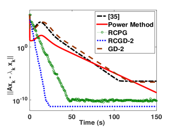
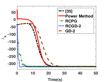
Figure 1: Behaviour along time (sec) of RCPG, RCGD-2, GD-2, algorithm [32] and power method on group Schenk IBMNA, matrix c-30: left - $\|Ax_{k}-\lambda_{k}x_{k}\|$, right - $\lambda_{k}$.

8.2 Matrix factorization

Finally, we consider the penalized orthogonal matrix factorization problem, see also [3]:

(84) $$\min_{(W,V)}F(W,V)=\min_{(W,V)}\dfrac{1}{2}\|X-WV\|^{2}_{F}+\dfrac{\lambda}{2}\|I-VV^{T}\|^{2}_{F},\vspace{-0.2cm}$$

with $W\in\mathbb{R}^{m\times r}$ and $V\in\mathbb{R}^{r\times n}$. Let us define: $f(W,V)=\dfrac{1}{2}\|X-WV\|^{2}_{F}$ and $\psi(W,V)=\dfrac{\lambda}{2}\|I-VV^{T}\|^{2}_{F}.$ Then, one can easily compute:

$$\nabla_{W}f(W,V)=WVV^{T}-XV^{T}\;\;\text{ and }\;\;\nabla^{2}_{WW}f(W,V)Z=ZVV^{T}.$$

Thus, $\nabla f$ is Lipschitz continuous w.r.t. $W$, with $L_{1}(V)=\|VV^{T}\|_{F}$. Similarly:

$$\nabla_{V}f(W,V)=W^{T}WV-W^{T}X\text{ and }\nabla^{2}_{VV}f(W,V)Z=W^{T}WZ.\vspace*{-0.2cm}$$

Therefore, $\nabla f$ is also Lipschitz continuous w.r.t. $V$, with constant Lipschitz $L_{2}(W)=\|W^{T}W\|_{F}$. On the other hand, $\nabla_{V}\psi(W,V)=2\lambda(VV^{T}V-V)$ and thus

$$\nabla^{2}_{VV}\psi(W,V)Z=2\lambda(ZV^{T}V+VZ^{T}V+VV^{T}Z-Z).\vspace*{-0.2cm}$$

Therefore, we get the following bound on the Hessian:

$$\langle Z,\nabla^{2}_{V}\psi(W,V)Z\rangle=\langle Z,2\lambda(ZV^{T}V+VZ^{T}V+VV^{T}Z-Z)\rangle\leq 6\lambda\|Z\|_{F}^{2}\|V\|_{F}^{2}.\vspace*{-0.2cm}$$

This shows that $\nabla^{2}_{V}\psi(\cdot)$ satisfies condition [A.4] in Assumption 4.1, with $p=2$ and $H_{\psi}=6\lambda$. Note that if we assume that there exist $\bar{L}_{1},\bar{L}_{2}>0$ such that $L_{1}(V)\leq\bar{L}_{1}$ and $L_{2}(W)\leq\bar{L}_{2}$, then Lemmas 4.2 and 4.4 are still valid. Therefore, we can solve problem (84) using algorithm CGD with the second stepsize choice (i.e., equation (LABEL:eq:HF2)) to update $V$. Moreover, since $\nabla F$ is Lipschitz continuous w.r.t. $W$, we can use algorithm CGD to also update $W$. Since we have only 2 blocks we consider the cyclic variant of CGD, named CCGD. Thus, the iterations of algorithm CCGD are:

$$W_{k+1} = W_{k}-\dfrac{1}{H_{f,W}(V_{k})}(W_{k}V_{k}V_{k}^{T}-XV_{k}^{T}),$$

$$V_{k+1} = V_{k}-\dfrac{1}{H_{F_{k}}}\left(W_{k+1}^{T}W_{k+1}V_{k}-W_{k+1}^{T}X+2\lambda(V_{k}V^{T}_{k}V_{k}-V_{k})\right),$$

with $H_{f,W}(V_{k})>\dfrac{L_{1}(V_{k})}{2}$, $H_{f,V}(W_{k+1})>\dfrac{L_{2}(W_{k+1})}{2}$, $H_{F_{k}}=12\lambda\|V_{k}\|_{F}^{2}+12\lambda\alpha_{k}^{2}+H_{f,V}(W_{k+1})$ and $\alpha_{k}$ is the positive root of the following third order equation:

$$12\lambda\alpha^{3}+\left(12\lambda\|V_{k}\|_{F}^{2}+H_{f,V}(W_{k+1})\right)\alpha-\|\nabla_{V}f(W_{k+1},V_{k})+\nabla_{V}\psi(W_{k+1},V_{k})\|_{F}=0.\vspace*{-0.2cm}$$

In our experiments, in CCGD-1 we take $H_{f,W}(V_{k})=0.51\cdot L_{1}(V_{k})$ and $H_{f,V}(W_{k+1})=0.51\cdot L_{2}(W_{k+1})$, while in CCGD-2 we take $H_{f,W}(V_{k})=L_{1}(V_{k})$ and $H_{f,V}(W_{k+1})=L_{2}(W_{k+1})$. We compare the two variants of CCGD algorithm with the algorithm BMM in [18]. For problem (84), BMM is a Bregman type gradient descent method having computational cost per iteration comparable to our method. For numerical tests, we consider SalinasA and Indian Pines data sets from [41]. Each row of matrix $X$ is a vectorized image at a given band of the data set. Each image is normalized to $[-1,1]$. The starting matrix $W_{0}$ is generated from a standard normal distribution $\mathcal{N}(0,1)$ and the matrix $V_{0}$ is generated with orthogonal rows. Moreover, we take $\lambda=1000$ and the dimension $r$ is taken as in [41] (i.e., in SalinasA we take $r=6$ and in Indian Pines we choose $r=16$). We run all the algorithms for $100$s. The results are displayed in Figures 2 (SalinasA) and 3 (Indian Pines), where we plot the evolution of function values (left) and the orthogonality error $O_{\text{error}}=\|I-V_{k}V_{k}^{T}\|_{F}$ (right) along time (in seconds). Note that in terms of function values CCGD is competitive with algorithm BMM. However, our algorithm identifies orthogonality faster than BMM.

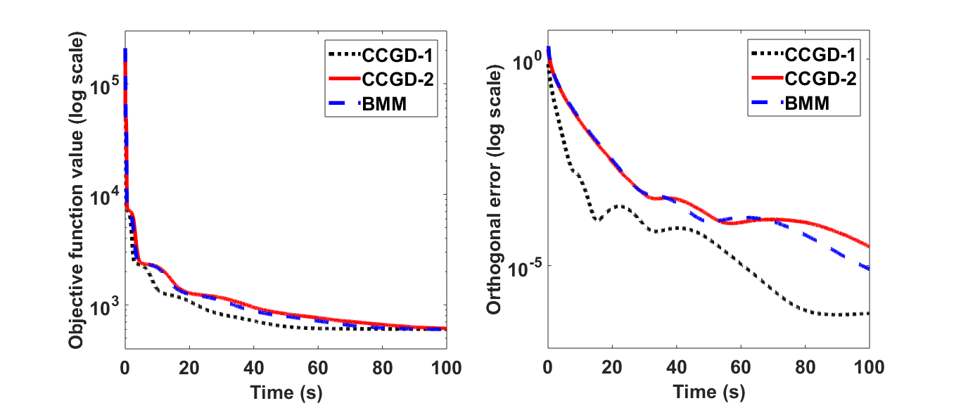
Figure 2: CCGD and BMM on SalinasA: left - function values, right - orthogonality error

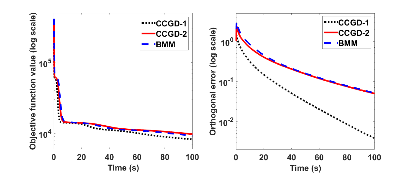
Figure 3: CCGD and BMM on Indian Pines: left - function values, right - orthogonality error.

9 Conclusions

In this paper we have considered composite problems having the objective formed as a sum of two terms, one smooth and the other twice differentiable, both possibly nonconvex and nonseparable. For solving this problem we have proposed two algorithms, a coordinate proximal gradient method and a coordinate gradient descent method, respectively. For the second algorithm we have designed several novel adaptive stepsize strategies which guarantee descent. For both algorithms we derived convergence bounds in both convex and nonconvex settings. Preliminary numerical results confirm the efficiency of our algorithms on real applications.

Acknowledgements. The research leading to these results has received funding from: TraDE-OPT funded by the European Union’s Horizon 2020 Research and Innovation Programme under the Marie Skłodowska-Curie grant agreement No. 861137; UEFISCDI PN-III-P4-PCE-2021-0720, under project L2O-MOC, nr. 70/2022.

Appendix

Recall that $\mathbbm{1}_{A}$ denotes the indicator function of the set $A$.

Lemma 9.1.

Let $(X_{k})_{k\geq 0}$ be a sequence of random variables on a probability space ($\Omega$,$\mathcal{F}$,$P$). Assume that exists $C_{0}>0$ such that $0\leq X_{k}\leq C_{0}$ with probability one for all $k\geq 0$. Let $\delta>0$ and a measurable set $\Omega_{\delta}\subset\Omega$ such that $P(\Omega_{\delta})\geq 1-\delta$. Then:

(85) $$\mathbb{E}[X_{k}]-C_{0}\sqrt{\delta}\leq\mathbb{E}[X_{k}\mathbbm{1}_{\Omega_{\delta}}]\leq\mathbb{E}[X_{k}]\quad\forall k\geq 0.$$

Proof 9.2.

Following an argument as in Lemma A.5 from [22], we have: $X_{k}=X_{k}\mathbbm{1}_{\Omega_{\delta}}+X_{k}\mathbbm{1}_{\Omega\backslash\Omega_{\delta}}.$ This implies that:

(86) $$\mathbb{E}[X_{k}]=\mathbb{E}[X_{k}\mathbbm{1}_{\Omega_{\delta}}]+\mathbb{E}[X_{k}\mathbbm{1}_{\Omega\backslash\Omega_{\delta}}].$$

Using Cauchy- Schwarz inequality, $X_{k}\leq C_{0}$, and $\mathbb{E}[\mathbbm{1}_{\Omega\backslash\Omega_{\delta}}]=P(\Omega\backslash\Omega_{\delta})\leq\delta$, we get:

(87) $$\mathbb{E}[X_{k}\mathbbm{1}_{\Omega\backslash\Omega_{\delta}}]\leq\sqrt{\mathbb{E}[X_{k}^{2}]}\sqrt{\mathbb{E}[\mathbbm{1}^{2}_{\Omega\backslash\Omega_{\delta}}]}\leq C_{0}\sqrt{\delta}.$$

From (86) and (87), we get the left hand side in (85). Moreover, since $X_{k}\geq 0$, we have $\mathbb{E}[X_{k}\mathbbm{1}_{\Omega\backslash\Omega_{\delta}}]\geq 0$ and using (86), we get the right hand side in (85).

Proof of Lemma 2.2. Consider a vector $u\in\mathbb{R}^{m}$, with $\|u\|=1$ and the parameterization $\alpha_{u}:[0,1]\to\mathbb{R}$ defined as $\alpha_{u}(t)=\langle G\left(x+tUd\right),u\rangle$. From mean value theorem, there exists $\bar{t}\in[0,1]$ such that $\alpha_{u}(1)-\alpha_{u}(0)=\alpha_{u}^{\prime}(\bar{t})$. This implies: $\langle G\left(x+Ud\right)-G\left(x\right),u\rangle=\langle J\left(x+\bar{t}Ud\right)Ud,u\rangle.$ Hence

$$|\langle G\left(x+Ud\right)-G\left(x\right),u\rangle|\leq\|J\left(x+\bar{t}Ud\right)Ud\|\|u\|\leq\|J\left(x+\bar{t}Ud\right)U\|\|d\|\|u\|.\vspace*{-0.2cm}$$

If we define $y=x+\bar{t}Ud$ and take $u=\dfrac{G\left(x+Ud\right)-G\left(x\right)}{\|G\left(x+Ud\right)-G\left(x\right)\|}$, we get the statement.

Proof of Lemma 6.10. We use a similar definition as in [36], i.e., let $\{\Delta_{k}^{\epsilon}\}_{k\geq 0}$ be the following sequence:

$$\Delta_{k}^{\epsilon}=\left\{\begin{array}[]{ll}\Delta_{k}\;\text{ if }\;\Delta_{k}\geq\epsilon,\quad\text{satisfies}\quad\Delta_{k}^{\epsilon}\leq\epsilon\iff\Delta_{k}\leq\epsilon\quad\forall k\geq\bar{k}.\\ 0\;\text{ otherwise,}\end{array}\right.\vspace*{-0.3cm}$$

Therefore, from Markov inequality, we have $\mathbb{P}\left[\Delta_{k}>\epsilon\right]=\mathbb{P}\left[\Delta_{k}^{\epsilon}>\epsilon\right]\leq\dfrac{\mathbb{E}[\Delta_{k}^{\epsilon}]}{\epsilon}.$ Hence, it suffices to show that $\theta_{K}\leq\epsilon\rho$, where $\theta_{k}:=\mathbb{E}[\Delta_{k}^{\epsilon}]$. If (72) holds, then

$$\mathbb{E}[\Delta_{k+1}^{\epsilon}]\leq\mathbb{E}[\Delta_{k}^{\epsilon}]-\mathbb{E}[\Delta_{k}^{\epsilon}]^{\zeta+1},\quad\mathbb{E}[\Delta_{k+1}^{\epsilon}]\leq\left(1-\epsilon^{\zeta}\right)\mathbb{E}[\Delta_{k}^{\epsilon}].\vspace*{-0.2cm}$$

Hence, we obtain $\theta_{k+1}\leq\theta_{k}-\theta_{k}^{\zeta+1}$ and $\theta_{k+1}\leq\left(1-\epsilon^{\zeta}\right)\theta_{k}$. Using now the inequality (28) of Lemma 9 in [26], we get $\left(k-\bar{k}\right)\zeta\leq\theta_{k}^{-\zeta}-\theta_{\bar{k}}^{-\zeta}$. Therefore, if we let $k_{1}\geq\dfrac{1}{\zeta}\left(\dfrac{1}{\epsilon^{\zeta}}-\dfrac{1}{\Delta_{0}^{\zeta}}\right)+\bar{k}$, we obtain $\theta_{k_{1}}\leq\epsilon$. Finally, letting, $k_{2}\geq\dfrac{1}{\epsilon^{\zeta}}\log\dfrac{1}{\rho}$, we have:

$$\theta_{K}\leq\theta_{k_{1}+k_{2}}\leq\left(1-\epsilon^{\zeta}\right)^{k_{2}}\theta_{k_{1}}\leq\left((1-\epsilon^{\zeta})^{\frac{1}{\epsilon^{\zeta}}}\right)^{\log\frac{1}{\rho}}\epsilon\leq\left(e^{-1}\right)^{\log\frac{1}{\rho}}\epsilon=\epsilon\rho,\vspace*{-0.2cm}$$

which proves our statement.

References

- [1] A. Aberdam and A. Beck An Accelerated Coordinate Gradient Descent Algorithm for Non-separable Composite Optimization, J. Opt. Theory and Appl., 193: 219–246 , 2021.
- [2] L. Armijo. Minimization of functions having lipschitz continuous first partial derivatives. Pacific J. Math., 16(1): 1–3, 1966.
- [3] M. Ahookhosh, L.T. K. Hien, N. Gillis and P. Patrinos, Multi-block Bregman proximal alternating linearized minimization and its application to orthogonal nonnegative matrix factorization, Computational Optimization and Application, 79: 681–715, 2021.
- [4] A. Beck, On the convergence of alternating minimization for convex programming with applications to iteratively reweighted least squares and decomposition schemes, SIAM Journal on Optimization, 25(1): 185–209, 2014.
- [5] A. Beck and L. Tetruashvili, On the convergence of block coordinate descent type methods, SIAM Journal on Optimization, 23(4): 2037–2060, 2013.
- [6] D. Bertsekas, Nonlinear Programming, Athena Scientific, 1999.
- [7] J. Bolte, A. Daniilidis and A. Lewis, The Łojasiewicz inequality for nonsmooth subanalytic functions with applications to subgradient dynamical systems, SIAM Journal on Optimization, 17: 1205–1223, 2007.
- [8] J. Bolte, S. Sabach and M. Teboulle, Proximal alternating linearized minimization for nonconvex and nonsmooth problems, Mathematical Programming, 146: 459–494, 2014.
- [9] S. Bonettini, Inexact block coordinate descent methods with application to non-negative matrix factorization, IMA Journal of Numerical Analysis, 31: 1431–1452, 2021.
- [10] Y. Carmon and J.C. Duchi, Gradient descent efficiently finds the cubic regularized nonconvex Newton step, SIAM Journal on Optimization, 29(3): 2146–2178, 2019.
- [11] D. Davis, The asynchronous PALM algorithm for nonsmooth nonconvex problems, arXiv preprint: 1604.00526, 2016.
- [12] T.A. Davis and Y. Hu. The University of Florida Sparse Matrix Collection, ACM Transactions on Mathematical Software 38(1): 1–25, 2011.
- [13] O. Fercoq and P. Richtarik. Accelerated, parallel and proximal coordinate descent, SIAM Journal on Optimization, 25(4): 1997–2023, 2015.
- [14] J. Friedman, T. Hastie, H. Hofling and R. Tibshirani, Pathwise coordinate optimization, The Annals of Applied Statistics: 1(2): 302–332, 2007.
- [15] L. Grippo and M. Sciandrone, On the convergence of the block nonlinear Gauss-Seidel method under convex constraints, Operations Research Letters, 26(3): 127–136, 2000.
- [16] D. Grishchenko, F. Iutzeler and J. Malick Proximal gradient methods with adaptive subspace sampling, Mathematics of Operations Research, 46(4): 1235–1657, 2021.
- [17] F. Hanzely, K. Mishchenko and P. Richtarik, SEGA: Variance Reduction via Gradient Sketching, Advances in Neural Information Processing Systems, 31, 2018.
- [18] L.T.K. Hien, D.N. Phan, N. Gillis, M. Ahookhosh and P. Patrinos Block bregman majorization minimization with extrapolation, SIAM Jounal on Optimization, 4(1): 1 – 25, 2022
- [19] P. Latafat, A. Themelis and P. Patrinos Block-coordinate and incremental aggregated proximal gradient methods for nonsmooth nonconvex problems, Math. Prog., 193: 195 – 224, 2021.
- [20] H. Lu, R.M. Freund and Yu. Nesterov, Relatively Smooth Convex Optimization by First-Order Methods and Applications, SIAM Journal on Optimization, 28(1): 333–354, 2018.
- [21] Z. Lu and L. Xiao, On the complexity analysis of randomized block-coordinate descent methods, Mathematical Programming, 152(1-2): 615–642, 2015.
- [22] R. Maulen, S.J. Fadili and H. Attouch, An SDE perspective on stochastic convex optimization, arXiv prepint: 2207.02750, 2022.
- [23] B. E. Meserve, Fundamental Concepts of Algebra, Dover, New York, 1982.
- [24] T. Mitchell, Machine Learning, McGraw Hill, 1997.
- [25] I. Necoara, Random coordinate descent algorithms for multi-agent convex optimization over networks, IEEE Transactions on Automatic Control, 58(8): 2001–2012, 2013.
- [26] I. Necoara and F. Chorobura, Efficiency of stochastic coordinate proximal gradient methods on nonseparable composite optimization, arXiv preprint: 2104.13370, 2021.
- [27] I. Necoara and D. Clipici, Efficient parallel coordinate descent algorithm for convex optimization problems with separable constraints: Application to distributed MPC, Journal of Process Control, 23(3): 243–253, 2013.
- [28] I. Necoara and D. Clipici, Parallel random coordinate descent methods for composite minimization: convergence analysis and error bounds, SIAM J. Opt., 26(1): 197–226, 2016.
- [29] I. Necoara and M. Takac, Randomized sketch descent methods for non-separable linearly constrained optimization, IMA Journal of Numerical Analysis, 41(2): 1056–1092, 2021.
- [30] Yu. Nesterov, Accelerating the cubic regularization of Newton’s method on convex problems, Mathematical Programming, 112: 159–181, 2008.
- [31] Yu. Nesterov, Efficiency of coordinate descent methods on huge-scale optimization problems, SIAM Journal on Optimization: 22(2): 341–362, 2012.
- [32] Yu. Nesterov, Inexact basic tensor methods for some classes of convex optimization problems, Optimization Methods and Software, doi: 10.1080/10556788.2020.1854252, 2020.
- [33] Yu. Nesterov and B.T. Polyak, Cubic regularization of Newton method and its global performance, Mathematical Programming, 108: 177–205, 2006.
- [34] Yu. Nesterov and S.U. Stich, Efficiency of the accelerated coordinate descent method on structured optimization problems, SIAM Journal on Optimization, 27(1): 110–123, 2017.
- [35] M.J.D. Powell, On search directions for minimization algorithms, Mathematical Programming, 4: 193–201, 1973.
- [36] P. Richtarik and M. Takac, Iteration complexity of randomized block-coordinate descent methods for minimizing a composite function, Mathematical Programming, 144: 1–38, 2014.
- [37] H. Robbins, and D. Siegmund, A convergence theorem for non-negative almost supermartingales and some applications, Optimizing Methods in Statistics, 233–257, 1971.
- [38] E. M. Stein and R. Shakarchi, Real Analysis: Measure Theory, Integration, and Hilbert Spaces, Princenton University Press, 2005.
- [39] P. Tseng and S. Yun, Block-coordinate gradient descent method for linearly constrained nonsmooth separable optimization, Journal of Optim. Theory and Applications, 140, 2009.
- [40] S.J. Wright, Coordinate descent algorithms, Mathematical Programming, 151(1): 3–34, 2015.
- [41] http://www.ehu.eus/ccwintco/index.php/Hyperspectral_Remote_Sensing_Scenes.