GPU-Powered Spatial Database Engine for Commodity Hardware: Extended Version

Abstract

Given the massive growth in the volume of spatial data, there is a great need for systems that can efficiently evaluate spatial queries over large data sets. These queries are notoriously expensive using traditional database solutions. While faster response times can be attained through powerful clusters or servers with large main-memory, these options, due to cost and complexity, are out of reach to many data scientists and analysts making up the long tail.

Graphics Processing Units (GPUs), which are now widely available even in commodity desktops and laptops, provide a cost-effective alternative to support high-performance computing, opening up new opportunities to the efficient evaluation of spatial queries. While GPU-based approaches proposed in the literature have shown great improvements in performance, they are tied to specific GPU hardware and only handle specific queries over fixed geometry types.

In this paper we present SPADE, a GPU-powered spatial database engine that supports a rich set of spatial queries. We discuss the challenges involved in attaining efficient query evaluation over large datasets as well as portability across different GPU hardware, and how these are addressed in SPADE. We performed a detailed experimental evaluation to assess the effectiveness of the system for wide range of queries and datasets, and report results which show that SPADE is scalable and able to handle data larger than main-memory, and its performance on a laptop is on par with that other systems that require clusters or large-memory servers.

1 Introduction

The widespread use of GPS-based sensors, IoT devices, phones and social media has resulted in an explosion of spatial data that is being collected and stored. Increasingly, data scientists and analysts are resorting to interactive analyses and visual tools to obtain insights from these data (e.g., [5, 15, 14, 4, 40]). However, executing queries involving complex geometric constraints over large spatial data sets is time consuming, and this greatly hampers users’ ability to interactively explore data. Commonly-used approaches, such as the spatial extensions available in existing relational database systems, even on powerful hardware, take from several minutes to run a single spatial selection query [12] to several hours for more complex queries such as joins [33]. While faster response times can be attained through powerful clusters and large memory servers, these options, due to cost and complexity, are often out of reach for analysts that make up the long tail; they are forced to work with small subsets of the data that can be handled in less powerful desktops and laptops. This raises an important question: can we support scalable spatial analytics for users in the long tail?

Modern graphics processing units (GPU) exhibit impressive computational power and provide a cost-effective alternative to support high-performance computing. For example, the Intel UHD GPU present in mid-range laptops reaches up to 0.5 TFLOPS, while the previous generation Nvidia GTX 1070 MaxQ mobile GPU reaches over 5 TFLOPS. Current-generation desktop and server GPUs are even faster, attaining speeds as high as 36 TFLOPS. Their wide availability, even in lower-end laptops, open up new opportunities to democratize large-scale spatial analytics. Not surprisingly, methods have been proposed to evaluate different types of spatial queries on the GPU [12, 49, 50, 51, 8, 41]. However, their adoption has not expanded beyond select research projects. We posit that this is due to two main reasons. First, no single system or library can both harness the power offered by GPUs and support the variety of queries commonly used in spatial analysis. Second, almost all current approaches use CUDA [26] and only work on Nvidia GPUs which are not always available in commodity hardware.

One possible approach would be to design a full-fledged GPU-based spatial query engine that combines existing approaches. But such a strategy quickly becomes unwieldy because existing methods target specific queries (e.g., selection over point data, or aggregation over polygons) and use custom data structures/indexes for each query type. This makes it difficult to reuse the data structures across different queries. Moreover, many of these approaches port CPU-based algorithms to the GPU. While general-purpose computing capabilities of GPUs have improved in recent times, traditional algorithmic constructs still cannot make optimal use of the parallelization provided by them, often leading to ineffective use of GPU capabilities.

The Spade Query Engine. To overcome these challenges, we propose Spade, a GPU-powered spatial query engine. By adopting the canvas data model and GPU-friendly algebra [10], Spade is able to support a rich set of query types. In addition, since the algebraic operators are adapted from common computer graphics operations for which GPUs are optimized, it is possible to harness the compute power provided by the hardware. Spade uses the computer graphics pipeline to implement the operators, and thus, it is portable and can be run on any GPU hardware.

There are several challenges involved in implementing the GPU-friendly algebra and data model to efficiently handle large spatial data sets on commodity hardware. First, the system must support datasets that do not fit in main memory. While the implementation of some of the algebra operators is straightforward, for others a naïve implementation leads to performance bottlenecks and the inability to handle large data due to memory limitations of the GPU. In addition, these operators involve costly geometric tests whose computational complexity is polynomial to the size of the geometries, and thus can negatively impact query execution time.

To design Spade, we adopted a computer-graphics perspective to evaluate spatial queries. We devised a methodology to implement the GPU-friendly operators [10] using the modern graphics pipeline [37], which enables both portability and efficiency. We show that, by using the GPU-based operators to efficiently query spatial indexes, Spade is able to handle large data sets that do not fit in memory. We also propose two canvas-specific indexes that both speed up geometry intersections and improve GPU occupancy.

Spade is designed to seamlessly support linkage to relational data and to be easily integrated with relational database systems. This is crucial since analytics over spatial data often requires a combination of relational and spatial queries. Spade also includes a query optimizer that specifies the order of operations for a given query plan and chooses the appropriate index and/or implementation for the different operators.

To assess the performance of Spade and its ability to handle large-scale analytics on commodity desktops and laptops, we perform an extensive evaluation using a wide range of queries and real data sets having as many as 100 million polygons and 2 billion points. The results show that Spade is scalable and efficiently handles data that is larger than main memory and that its performance is comparable to that of cluster-based and large memory solutions. Specifically, Spade running on a laptop equipped with a Nvidia 1070 MaxQ GPU performs on par with both GeoSpark [48] running on a 17 node cluster, as well as in-memory spatial libraries [17] running on large main-memory servers. We also discuss insights uncovered during the evaluation into how to further improve Spade as well as how to combine it with the existing solutions.

Contributions. We introduce Spade which, to the best of our knowledge, is the first GPU-powered spatial database engine that supports the evaluation of a rich set of spatial queries over different GPU hardware. Given its ability to efficiently handle complex queries over big data on commodity hardware, Spade has the potential to make large-scale spatial data analysis widely accessible. To summarize:

• We demonstrate how the canvas model and the spatial algebra [10] can be realized using the computer graphics pipeline to attain efficiency, accuracy, portability, and scalability on commodity hardware.

• We propose two indexes designed to support the canvas model: the boundary index that enables constant time geometry intersection tests, and the layer index that speeds up spatial join queries by improving the GPU occupancy.

• We describe the architecture and implementation of the Spade system and show how it can be integrated with existing relational systems, how existing disk-based spatial indexes can also be queried using the GPU operators, and how query execution can be optimized.

• We present results of an extensive experimental evaluation of Spade which demonstrate its efficiency.

2 Background

To provide context we first give a brief informal overview of the canvas data model and GPU-friendly spatial algebra [10]. We refer the reader to [10, 11] for details. We then describe the shader-based computer graphics pipeline [37] that is used to implement Spade.

2.1 Spatial Data Model and Algebra

The canvas data model and GPU-friendly algebra [10] were designed to exploit GPUs for executing spatial queries. Intuitively, the canvas data model [10] can be thought of as a “drawing” of the geometry, and is represented as a collection of images. However, unlike traditional images, each pixel of a canvas model image is designed to store the necessary metadata to both identify the geometry it represents as well as to support query execution. This model provides a uniform representation for spatial objects – not only points, lines, and polygons, but also any combination of these primitives.

The main advantage of the above representation is that it naturally allows the parallel execution of the GPU-friendly operators defined by the algebra. In particular, the algebra consists of five fundamental operators, inspired by common computer graphics operations. Figure 3 illustrates the operators implemented in Spade.

1. Geometric Transform: moves geometric objects in space.

2. Value Transform: modifies a geometric object’s properties.

3. Mask: filters regions based on a given mask condition.

4. Blend: merges two canvases into one.

5. Dissect: splits a canvas into a collection of non-empty canvases.

In addition to these, the algebra also includes derived operators that are compositions of one or more fundamental operators. These include the Multiway Blend operator, that applies several blends to merge multiple canvases, and the Map operator that is a composition of a dissect followed by a geometric transform. Spatial queries are realized by composing one or more of the above operators. For example, consider the spatial selection query that selects all geometric objects intersecting a polygonal constraint. This is realized by first blending the canvas corresponding to a geometric object with the canvas representing the query polygon, and then applying the mask operator that removes objects outside the query polygon. The first step creates an image that merges the query polygon and the input geometry into a single canvas, and the second step removes any geometry that is present outside the query polygon. The non-empty canvases that remain after the above two operations correspond to the query results. Note that the above composition of operators work on any geometric primitive. As described in Section 5.2, other spatial queries can be realized in a similar fashion.

2.2 The Computer Graphics Pipeline

Graphics intensive applications, such as games, involve rendering complex scenes that continuously change based on end-user interactions. These scenes are rendered as a collection of frames, where each frame contains the geometric objects as seen from a camera at a given time stamp. To obtain smooth transitioning between the frames, it is critical to have a high frame rate, i.e., a large number of frames rendered per second. GPUs are designed to speedup precisely these operations which are executed through the computer graphics pipeline – a high-level interface that allows the use of the underlying GPU hardware, while the GPU drivers handle low-level tasks such as optimizing for the GPU architecture (e.g., handling rasterization, threads).

OpenGL [37] (cross platform), Direct3D [24] (Microsoft Windows), metal [23] (OSX), and the more recent Vulkan [20] (cross platform) are some of the popular application programming interfaces (API) that support the computer graphics pipeline. This pipeline (also known as the shader pipeline) is divided into a set of stages that can be customized by the developer through the use of shaders.

Vertex Shader. The first stage of the pipeline is used to process the set of individual vertices that form the geometric primitives to be rendered. It supports three types of geometric primitives—points, lines and triangles (polygons are rendered as a collection of triangles). This stage is used to convert vertex coordinates into a common screen space (the coordinate system w.r.t. the camera), known as model-view-projection.

Custom Geometry Creation. This is an optional stage which is used to create custom geometries. Either the tessellation shader or the geometry shader can be used for this purpose. This stage takes as input the vertices output from the vertex shader together with optional user-defined parameters, and outputs zero or more new geometric primitives.

Vertex Post Processing. This stage is handled by the GPU (driver) and is used for clipping and rasterization. Clipping is the process where primitives outside the viewport (the space corresponding to the region visible from the camera) are removed, while those (lines and triangles) that are partially outside are cropped resulting in a new set of primitives that are fully contained within the viewport.

Rasterization is the process that converts each primitive within the viewport into a collection of fragments. Here, a fragment can be considered as the modifiable data corresponding to a pixel. The fragment size therefore depends on the resolution (width and height in terms of the number of pixels that form the screen space). Given the crucial part it plays in the graphics pipeline, GPU hardware vendors optimize parallel rasterization by directly mapping computational concepts to the internal layout of the GPU. Since all the primitives are simple (lines or triangles), identifying fragments that form a given primitive is amenable to hardware implementation.

Fragment (or Pixel) Shader. This stage allows custom processing for each fragment that is generated by the rasterizer. It is typically used to compute and set the “color” and “depth” (distance from the camera) for the fragment. Depending on the required functionality, it can also be used for other purposes (e.g., to discard fragments, write to additional output buffers).

Post Fragment Processing. The final stage of the pipeline processes the individual fragments output from the fragment shader to generate the pixels of the image corresponding to the scene being rendered. It is responsible for performing actions such as alpha blending (when objects have translucent material, then the colors of obstructing objects are blended together based on a blend function).

Virtual Screen. Graphics APIs also allow results to be output to a “virtual” screen, which is represented using a frame buffer (also called frame buffer object or FBO). Thus, rendering can now be performed without the need of a physical monitor. Even though the resolutions supported by existing monitors are limited, current generation graphics hardware supports frame buffers with resolutions as large as 32K $\times$ 32K.

Each pixel of this FBO is represented by 4 values $[r,g,b,a]$, corresponding to the red, blue, green, and alpha color channels. Each FBO is associated with a texture that stores the actual image.

3 SPADE: System Overview

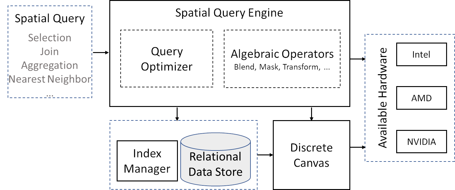
Figure 1: Spade system architecture.

The architecture of Spade, shown in Fig. 1, consists of four main components which we describe below. Note that since Spade is implemented using the computer graphics pipeline, it can run on any GPU hardware.

Relational Data Store. All data, indexes, and meta-data used by Spade are stored as relational tables. For our initial implementation, we use the embedded column store MonetDBLite [35] which provides a simple C API to load and store data using SQL. However, since the data is accessed using SQL, it is straightforward to integrate Spade with other database systems.

Discrete Canvas Creation. This component is responsible for creating canvases – the data used by the spatial operators. In Section 4, we outline how a discrete canvas can be created using the shader pipeline, and describe how to ensure accurate queries in spite of using rasterization to generate this canvas. Spade supports data sets comprising of common geometric primitives—points, lines, and polygons.

Spatial Query Engine. The spatial query engine, described in Section 5, forms the core of Spade and is responsible for planning, optimization, and execution of spatial queries.

Index Manager. Spade maintains two types of indexes that are used during the execution of spatial queries:

1. Canvas-specific indexes speed up spatial intersection tests and reduce the number of canvases that are created respectively, thus making spatial operations on the GPU more efficient (see Section 4.3).

2. The disk-based index supports out-of-core queries – the current version of Spade stores the underlying spatial data using a clustered grid index. However, as discussed in Section 7, other indexing strategies can be easily integrated with Spade.

4 Discrete Canvas

The canvas, when rasterized by the GPU, can lead to inaccurate query results. To overcome this limitation, we formalize the notion of discrete canvas in Section 4.1 and describe its creation using the rasterization-based pipeline in Section 4.2. Finally, in Section 4.3, we introduce canvas-specific indexes that we designed to speedup query processing.

4.1 Rasterized Canvas Representation

Using the rasterization-based pipeline, the Euclidean space is divided into a set of pixels. Thus, a trivial implementation of the canvas would have each pixel map to the necessary metadata. This metadata is defined as a triple of triples (or a $3\times 3$ matrix) [10], where each triple stores information corresponding to the three primitive types (point, line, polygon) respectively, that makeup a geometric object. However, this would result in inaccuracies due to the discretization caused by rasterization: since a pixel need not lie entirely within a geometry, this would induce errors for pixels that partially intersect the geometry.

We therefore extend the formal model from [10] to define a discrete canvas that uses a triple of 4-tuples(or a $3\times 4$ matrix). Here, for each 4-tuple $(v_{0},v_{1},v_{2},v_{b})$, $v_{0},v_{1}$, and $v_{2}$ are the same as in the original definition, and $v_{b}$ stores the necessary boundary data – a pointer to the boundary index that is used to obtain accurate query results (see Section 4.3). Intuitively, the discrete canvas can be thought of as a “localized” grid index corresponding to each geometric object. As mentioned earlier, each pixel of the texture associated with an FBO can store 4 values corresponding to the 4 color channels—this 4-tuple directly maps to the color channels of a pixel. Thus, to represent the canvas on the GPU, we use 3 textures, one for each primitive type.

4.2 Canvas Creation

Spade uses canvases to represent both data and query constraints. In our implementation, instead of storing all canvases associated with a data set, we create them on the fly as needed. The advantages of this approach are twofold. First, the data can be stored in the database in its vector format, thus reducing the space overhead. Second, depending on the query constraints, it is possible to realize the canvas for only a subset/sub-region of the data, often making it more efficient to render than load a pre-stored canvas. This is because the memory overhead of the serialized canvas is typically much higher, making it more costly to transfer the data from CPU to GPU as compared to data stored in a vector format. In what follows, we describe how canvases are created for different types of geometries.

Canvases for Traditional Primitives. We use the shader pipeline consisting of the vertex and fragment shaders to create canvases corresponding to traditional geometric primitives, i.e., points, lines, and polygons. Polygons are first decomposed into a set of triangles. We use the ear clipping based approach implemented in the Earcut.hpp library [22] for this purpose.

The vertex shader takes as input the coordinates of the vertices that make up the geometry (end points of the lines in case of lines, and vertices of the triangles in case of polygons) together with a unique identifier of the geometric object they are part of. A transformation matrix is also passed to the vertex shader, that converts the vertex coordinates that fall within the valid query region to the range $[-1,-1]\times[-1,-1]$ (Section 5 describes how this region is defined). Any additional coordinate system projection (e.g., converting from degree based EPSG:4326 coordinate system to the meter-based EPSG:3857 coordinate system) is also performed in the vertex shader.

The fragment shader then creates the canvas by writing the object identifier to the texture attachment in the FBO corresponding to the primitive being processed. Note that the fragments processed in the fragment shader correspond only to the primitives within the query region due to the clipping performed by the vertex post processing stage. For lines and polygons, in addition to the object identifier, the pointer to the boundary index is also written to the texture. For polygons, this process is done in two passes. The first pass renders the triangles, while the second pass renders the lines forming the polygon boundaries. The pointer to the boundary index is written only in the second pass.

To accurately identify all boundary pixels, we use the conservative rasterization feature provided by the graphics API. Conservative rasterization identifies and draws all pixels that are touched by a line (or triangle), and is different from the default rasterization, wherein pixels not satisfying the necessary intersection condition are not drawn.

Optimizing for Rectangular Range Queries. The constraints for these queries consist of axis parallel rectangles. Thus, given a rectangle, it is sufficient to store its diagonal endpoints. To create a canvas, we first convert each rectangle into two triangles using the geometry shader, and then use the same fragment shader that was used for polygon primitives above.

Canvases for Distance-Based Queries. Distance constraints are converted into polygonal constraints. In particular, we use geometry shaders to create these (query) polygons as follows. When the query is with respect to the distance $r$ from a point, the constraint is a circle which is generated by: 1) using the point coordinate and distance $r$ in the geometry shader to create a square of size $2r$ centered at the point, and then 2) the fragment shader identifies and draws the interior and boundary of the required circle within this square.

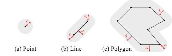
Figure 2: Distance canvases for different primitive types.

In the case of lines, a “rounded rectangle” is generated using the geometry shader. Given a line and a distance $r$, this polygon corresponds to a rectangle parallel to the line together with semicircles at the two endpoints as illustrated in Fig. 2(b). For polygons, the query constraint is generated by drawing the polygon interior followed by the boundary lines using the same geometry shader used above for lines (see Fig. 2(c)). This construction ensures that all points that fall inside the generated polygon will have their closest distance less than or equal to the distance constraint.

Computing distances to such complex geometries (such as in Fig. 2(c)) is traditionally a costly operation, due to which existing systems (e.g., GeoSpark [48]) typically define the distance to a line (or polygon) based on the distance to its center. On the other hand, Spade can accurately execute these queries—the only overhead is canvas creation which is small due to the use of geometry shaders.

4.3 Canvas-Specific Indexes

We propose two index structures that can be used together with the canvas-based spatial model to speedup query processing. In Section 5, we also show how the GPU-friendly operators defined in [10] can be used to create these indexes.

Boundary Index. A common operation across spatial queries is to test whether a given location intersects a geometric object. This is trivial if the corresponding pixel on the canvas is completely inside or outside the object. However, if the location falls on a boundary pixel, it is necessary to explicitly compute the intersection to enable accuracy. This is typically accomplished using costly point-in-polygon, line-polygon, or polygon-polygon intersection tests, each of which have time complexity polynomial in the size of the primitives (i.e., the number of vertices making up the primitive).

The first index we propose is the boundary index which serves two important purposes: 1) enable boundary tests necessary for accurate queries; and 2) speed up spatial intersection tests. The index is defined as a lookup table where the entries correspond to a geometric primitive that can be used to verify whether a point falling within a boundary pixel of the canvas intersects the geometry.

For points and lines, this lookup table is trivially defined: the point coordinates and the line end-point coordinates form the necessary entries, and the $v_{b}$ value of the boundary pixel of a canvas points to the corresponding entry in the table. In other words the data itself becomes the boundary index.

In the case of polygons, the lookup table stores the triangles making up the polygon together with the unique identifier of the geometry. In addition, we also store a mapping that associates every edge of a polygon to the triangle incident on it. For example, consider the polygon $P$ in Fig. 4. It consists of 4 boundary edges, of which $e_{1}$ and $e_{2}$ map to the triangle $t_{1}$, while the other two edges map to triangle $t_{2}$. This mapping is used during canvas creation to associate each boundary pixel (part of a polygon edge) to the corresponding triangle. Now, if a geometric primitive intersects with a boundary pixel, to test whether it also intersects with the corresponding polygon, it is sufficient to simply test if that primitive intersects the triangle indexed by that boundary pixel. For example, to test whether the cyan point intersects $P$ in Fig. 4, it suffices to simply test whether this point intersects $t_{1}$. Thus, costly point-in-polygon, line-polygon, and polygon-polygon intersection tests now become constant time point-triangle, line-triangle, and triangle-triangle tests, respectively. Brinkhoff et al. [7] had tried out similar index structures where the polygons were partitioned into either smaller convex polygons, trapezoids, or triangles, which were then stored using the R-tree. As they mention, this would still require $O(n)$ time in the worst case.

Layer Index. Recall that each geometric object is represented using one canvas. Thus, when working with data involving millions of objects, the operators need to be executed on millions of canvases. The goal of the layer index is to reduce the number of canvases created and used, and thus improve the query performance. In addition, it also improves the GPU occupancy since it allows multiple objects to be processed simultaneously. It is primarily defined for line and polygon primitives. Given a set of geometric objects (lines or polygons) that form a canvas, this index partitions the data into a set of layers, such that no two geometric objects in a given layer intersect. Note that in the worst case, when all objects intersect, each object is in its own layer which results in the same performance as having no layer index. However, such a scenario is rare in real world data, thus providing significant query speedup in practice.

5 Spatial Query Engine

The spatial query engine handles planning, optimizing, and executing the queries. In this section, we first discuss the shader-based implementation of the algebraic operators that are used for different queries–for their formal definitions, see [10]. We then describe in detail the query evaluation and optimization strategy followed for the different spatial queries. Finally, we show how the canvas-specific indexes introduced above can be computed using the GPU operators.

5.1 Implementing the Algebra Operators

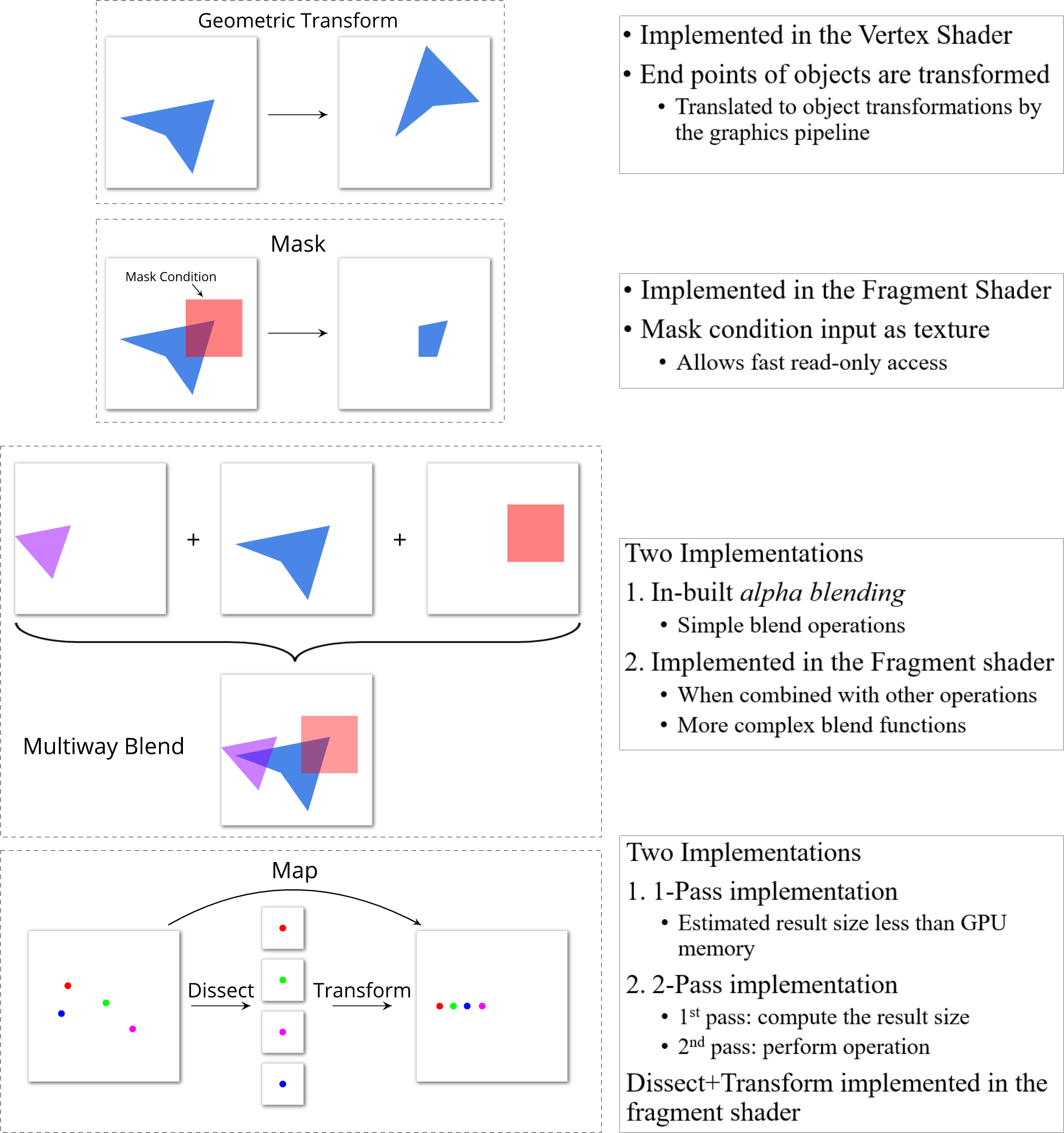
Figure 3: Operators implemented in Spade

Spade implements the following four operators that are summarized in Fig. 3.

Geometric Transform. When a canvas is created, the vertex shader performs the geometric transformation on the coordinates of the geometries to convert them into screen space. Here, the screen space is defined based on the query inputs and parameters (e.g., bounds of the selection query polygon), thus clipping (and not processing) regions that are not touched by the query (e.g., see Fig. 4). It is also used to change the coordinate system of the underlying data, in particular, from the latitude-longitude based coordinates to the meters-based EPSG:3857 coordinates for distance and $k$NN queries.

Mask. The mask operation is implemented in the fragment shader. Fragments are processed in parallel by the fragment shader, where they are tested against the mask condition. When this condition corresponds to a polygonal constraint, the corresponding constraint canvas together with the boundary index is used by the shader to test the mask condition (e.g., see Fig. 4). If the fragment falls on a boundary pixel, then the appropriate boundary tests are performed. To reduce memory lookup latency, Spade stores the constraint canvas in the part of the GPU memory that is segregated for textures. Since textures are read-only, hardware optimizations allow faster data access as compared to traditional global memory.

Multiway Blend. Since spatial data sets are made up of multiple canvases, a single multiway blend operator becomes beneficial compared to executing multiple blend operations. Hence, Spade implements the multiway blend operation. For simple blend functions such as additions (used for aggregations), we use the API-provided alpha blending operation. When the blend function is more complex, or in cases where blend is combined with other operations, we perform the blending in the fragment shader. The latter scenario is common when a blend is followed by a mask in a query plan. Since the operations are executed by explicitly rendering (drawing) the appropriate data, instead of having two (or more) rendering passes, one to perform blend and one to perform mask, combining the two operations into a single fragment shader helps avoid unnecessary rendering passes.

Map (Dissect + Geometric Transform). Since the dissect operation is never used in isolation in any of the queries, we chose to implement the Map operation as a single operator that performs a dissect followed by a geometric transform. By definition, the Map operation creates a canvas with a single point for each non-null fragment of a canvas, where the coordinates of the point are determined by the fragment values. This results in the creation of numerous canvases, and a naïve implementation becomes expensive.

One approach to overcome this is to implicitly represent each generated canvas within a single output canvas. Since each of the generated canvases has only one valid point, if we can store each of these points using unique pixels, then a single output canvas is sufficient. We accomplish this by using the identifiers associated with the generated canvases to uniquely encode the pixels in the output.

We have two distinct implementations of the Map operation, and the query optimization strategy chooses the appropriate implementation at runtime based on the query parameters:

1. Given estimate $n_{max}$, the maximum possible count of points that are generated by the dissect operation (described in the following section), a canvas with texture size (resolution) equal to $n_{max}$ is created, and the Map operation stores each created point at a unique location within this canvas. This canvas can be thought of as a list of size $n_{max}$ having both null and non-null values. When the query is complete, a GPU-based parallel scan operation [18] is executed (to remove the null elements of the list) and return the result.

2. When the maximum count cannot be estimated, then the Map operation is performed in two steps. The first step performs a simulated Map operation, counting the number of points created. This count is then used in the second step to perform the actual Map operation. Note that the second step may require multiple iterations depending on the count of the points computed in the first step.

5.2 Query Evaluation

Spade closely follows the query plans described in [10, 11] for the different spatial queries. Next, we describe the design choices made in our implementation for the different query types when the data fits into GPU memory. The following section details how this is extended for off-core processing of large data sets.

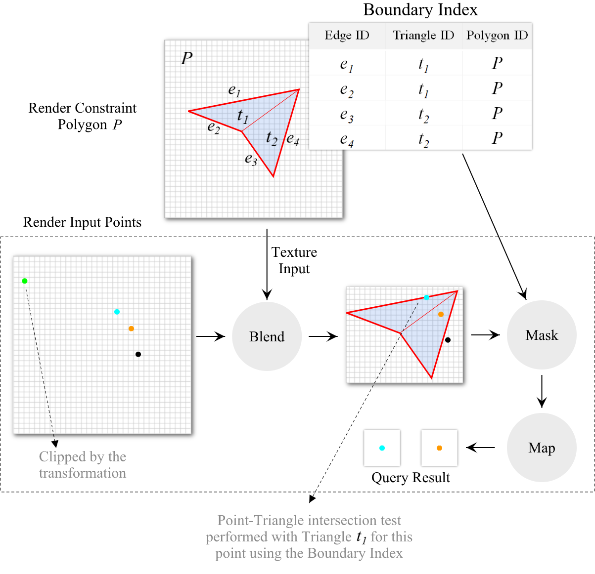
Figure 4: The steps executed for a selection query. The triangulated polygon is rendered and passed as a texture during the point rendering phase. As each point is rendered, if it falls outside the bounding box of the polygon (green point), it is clipped. Points that are not clipped then undergo the blend, mask, and map operations in the fragment shader. During the mask operation, if the point (cyan point) falls on a boundary pixel (bold red lines), then a point-triangle intersection test is performed using the boundary index.

Spatial Selection. A spatial selection query identifies all geometric objects from a given query data set that satisfies a spatial constraint and a select condition. Here the geometric objects can be points, lines, or polygons, or any combinations of these. Spade currently supports intersection (analogous to the SQL ST_INTERSECTS condition), when the spatial constraint is a polygon. In Section 7, we discuss the use of the containment (SQL ST_CONTAINS) condition. The original query plan used for spatial selection [10] performs a blend followed by a mask operation to generate a set of result canvases. To extract the query result from the result canvases, we use a modified plan that performs a Map operation following the mask. This query is implemented in three steps as illustrated in Fig. 4:

1. Create a canvas for the polygonal constraint and store it as a texture. This is done in one rendering pass.

2. Create canvases for the query data set. This is also accomplished in a single rendering pass as follows: All geometric objects are simultaneously drawn in this rendering pass. Each fragment is subjected to the blend and mask operation, and if the mask condition is satisfied, then the Map operation stores the data onto an output canvas. This way, the object canvases need not be stored and can be discarded immediately after the fragments are processed. The query constraint canvas, stored as a texture, is used by the fragment shader to accomplish the mask operation. Only objects within the query region defined by the bounding box of the constraint polygon are processed in this step. This is accomplished by defining a transformation of the input that clips (discards) any object outside this extent, and thus avoiding unnecessary processing.

3. The scan algorithm is used to extract the query result from the output canvas.

Spatial Joins. A spatial join between two spatial data sets, $D_{1}\bowtie D_{2}$ is implemented as a collection of spatial selections, where the selection constraint is from one of the data sets. The in-memory based implementation of the join query uses the layer index, introduced earlier. We look at how this is accomplished for the following two join scenarios:

(1) Polygon $\bowtie$ Point: Let $D_{1}$ be the polygon data set and $D_{2}$ be the point data set. Due to the layer index, each layer of $D_{1}$ contains polygons that do not intersect, and thus can be represented in a single canvas texture. Let there be $l$ layers in the layer index of $D_{1}$. The implementation then performs $l$ select operations one for each layer.

(2) Polygon $\bowtie$ Polygon: Here, both $D_{1}$ and $D_{2}$ are polygonal data sets. Let $l_{1}$ and $l_{2}$ be the number of layers respectively in the two data sets. Without loss of generality, let $l_{1}\leq l_{2}$. Similar to the previous scenario, $l_{1}$ selection operations are executed for each of the layers in $D_{1}$.

Distance-Based Queries. Distance-based selections and joins differ from spatial selections and joins only in Step 1: the constraint canvases are created using the geometry shader as defined in Section 4.2.

We support two types of distance-based joins, which are also executed similar to spatial joins:

(1) Given data sets, $D_{1},D_{2}$, and a distance $r$, the join returns all pairs of objects $(x_{i},y_{j})$ such that $x_{i}\in D_{1}$, $y_{j}\in D_{2}$ and $\text{distance}(x_{i},y_{j})\leq r$. The data set with the smaller number of elements is used for creating the constraint canvases.

(2) Given data sets, $D_{1},D_{2}$, and a set of distances $\{r_{1},r_{2},\ldots,r_{n}\}$, $n=|D_{1}|$, the join returns all pairs of objects $(x_{i},y_{j})$ such that $x_{i}\in D_{1}$, $y_{j}\in D_{2}$ and $\text{distance}(x_{i},y_{j})\leq r_{i}$. In this case, constraint canvases are created on $D_{1}$.

Since the distance parameter of the join query is provided together with the query, unlike polygonal data sets, it is not possible to have the layer index built beforehand – instead the index is built on the fly during query execution.

Spatial Aggregations. We support two implementations for the aggregation query. The first performs the necessary join (or select) followed by the count operation which is accomplished using a geometric transformation followed by a multiway blend. Here, the results from the select (or join) are moved to a unique location by the geometric transformation, and the blend operation counts the objects in each of these unique locations to obtain the aggregation result. The second implementation, follows the alternate query plan described in [11, Section 5.2]. This plan is customized for aggregations over point data, and uses the multiway blend, mask, and map operators. This plan first computes partial aggregates of the data using multiway blend, which are then combined together using the mask and map operations to generate the final result. Query speedup is obtained in this scenario by avoiding the materialization of the join (or select) results. This is possible only for points since any given point can be in at most one pixel of the canvas. Note that the latter implementation is always chosen by the optimizer when working with point data sets.

$k$NN Queries. Since common real-world $k$NN queries as well as existing spatial engines support $k$NN queries only over point data, we chose to customize the query plan used for $k$NN queries with respect to point data as well. Given a spatial data set $D$, consider a $k$NN selection query that identifies $k$ points closest to a query point $p$. Let $B$ be the bounding box of $D$. Let $r_{max}$ be the maximum distance from $p$ to the endpoints of $B$. The $k$NN query is then executed in 3 steps:

1. A circle data set $C$ with $c$ circular constraints is generated, where every circle has center $p$, and $i^{\text{th}}$ circle has radius $r_{i}=\frac{r_{max}}{\alpha^{i}}$, $0\leq i\leq c$ and $\alpha$ is a constant $>1$. Distance-based canvases are used for this purpose. A spatial aggregation query is then run on $D$ using $C$ as the constraints. Note that such an approach might seem inefficient from a traditional CPU algorithmic perspective. However from a computer graphics perspective, it is designed to harness the GPU as follows. The plan used for aggregation query above requires just one pass over the polygon constraints irrespective of the number of constraints in the query. In terms of graphics operations, this amounts to drawing the set of polygons once. GPUs are primarily designed for this operation. Since (i) polygons in this case are simple circles rendered efficiently using geometry shaders (Section 4.2); and (ii) the number of circles created is logarithmic on the spatial extent of the input in terms of the canvas resolution, which in practice is at most a few hundreds, the performance overhead of this step is small.

2. Let $r_{i}$ be the radius of the circle such that aggregation$(c_{i})\geq k$ and aggregation$(c_{i-1})<k$. A distance-based selection is now run on $D$ with $r_{i}$ as radius.

3. The query results are then sorted based on the distance to point $p$, and the $k$ closest points are selected from the sorted list.

A $k$NN join is executed similar to the $k$NN selection query. Let $D_{1}$ and $D_{2}$ be the input data sets. Let the query require identifying the $k$ nearest neighbors of points in $D_{1}$. Then, the circle data set containing circles with varying radii is created for each of the points in $D_{1}$ in the first step to identify the appropriate radius for each point in $D_{1}$. Then the Type 2 distance join is performed using the computed radii in Step 2. Finally, similar to the $k$NN selection query, the query results are sorted based on distance and the required result is computed.

5.3 Out-of-Core Queries

We now discuss how the above query strategies are extended to data that do not fit in GPU memory (and may or may not fit in CPU memory).

Grid-based index filtering. Spade uses a clustered grid-based indexing structure where each grid cell corresponds to a block of data that falls into that cell. The block size is tuned based on the system configuration to ensure that any given grid cell fits into GPU memory (see Section 6.1). The collection of non-empty grid cells is stored as a set of bounding polygons, i.e., for each cell, instead of storing simply the bounding box, we store the convex hull over the geometries present in that cell. Thus, the index itself forms a polygonal data set. When an object spans more than one cell, it is added to the cell that contains its centroid and the cell’s boundary is expanded. Thus, the cells themselves could intersect unlike in a traditional grid index. The filtering is then accomplished by executing the appropriate selection/join query on this set of boundary polygons. Thus, having intersecting cells does not affect the query evaluation strategy.

Due to the use of more detailed polygons instead of bounding rectangles, the index filtering stage of query execution filters out more data, thus reducing the amount of data used for the refinement stage. Such a strategy is not used in a traditional setting due to the high processing cost this filtering incurs. However, the overhead is low in our case since this representation enables the reuse of GPU-based selections and joins to perform fast index filtering.

Next, we describe the query execution strategy for spatial selections and joins. Other queries are also executed using a similar strategy. Note that when the data does not fit in CPU memory, the cells of the index are memory mapped and loaded into the CPU as and when necessary

Spatial Selection. In the index filtering phase of the query, a spatial selection query is first executed on the bounding polygons (corresponding to the cells) of the clustered grid index to identify all grid cells that satisfy the selection constraint. For the refinement phase, the GPU in-memory spatial selection query is then executed on each of these grid cells.

Spatial Joins. Spade incorporates two strategies to perform spatial joins over out-of-core data. The first makes use of the layer-index based in-memory join described above as follows. Let $D_{1}$ and $D_{2}$ be the two data sets used for the spatial join. The filter phase first performs a Polygon $\bowtie$ Polygon join over the bounding polygons of the indexes corresponding to $D_{1}$ and $D_{2}$ respectively. This join returns all pairs of grid cells $(g_{i}^{1},g_{j}^{2})$, where $g_{i}^{1}\in D_{1}$ and $g_{j}^{2}\in D_{2}$.

A spatial join is then executed for each pair of grid cells.

The second strategy follows a naïve approach that implements it as a loop of selects. Even though the use of the layer index decreases the number of canvases involved in the join, since multiple polygons are part of a single layer (and hence canvas), these layers can cover a large region. Say, data set $D_{1}$ contains such large-extent layers, then for each layer, data corresponding to large extents from $D_{2}$ needs to be transferred to the GPU. On the other hand, if the individual polygons in $D_{1}$ cover a relatively smaller region, then depending on the distribution of the data in $D_{1}$ and $D_{2}$, the total data transferred to the GPU can be significantly lower when summed over all polygons in $D_{1}$. While the layer index-based approach optimizes for the number of rendering passes, it does not consider the memory transfer. Since the data transfer forms the primary bottleneck in query execution times, the naïve strategy can therefore perform better in such scenarios.

5.4 Query Optimization Strategies

Spade implements a query optimizer (QO) that performs the following tasks:

Select the appropriate Map operator implementation. The Map operation has two implementations as described above. It is primarily used to consolidate the results of a query. When the estimate of the query result ($n_{max}$) is small enough to fit into the maximum memory allocated for a single canvas, then the 1-pass Map implementation is used. Otherwise, the 2-pass implementation is used. The result estimation for the different queries is performed as follows:

1. Selection query: Since each object can either satisfy the query constraint or not, the maximum size of the output, $n_{max}$, is equal to the number of objects.

2. Join query: First, consider Polygon ($D_{1}$) $\bowtie$ Point ($D_{2}$) joins. Let the number of polygons in $i^{\textrm{th}}$ layer of the $D_{1}$’s layer index be $m$, and number of points in $D_{2}$ be $n$. The estimate for $n_{max}$ in this case is $n$ since no two polygons intersect within a given layer, and a point can intersect only one polygon.

In case of Polygon ($D_{1}$) $\bowtie$ Polygon ($D_{2}$) joins, let the number of polygons in $i^{\textrm{th}}$ layer of $D_{1}$ be $m$, and number of polygons in $D_{2}$ be $n$. Unlike the previous scenario, the estimate of $n_{max}$ is now $n\times m$ (a single polygon in $D_{1}$ can intersect multiple polygons in $D_{2}$).

Choose the join implementation. Recall that when a join query is invoked on data sets that do not fit in memory, Spade supports two join implementations: a naïve approach of executing a set of selections, and using the layer index. To choose the implementation to be executed, the QO first computes the amount of data that needs to be transferred to the GPU. For the naïve approach, this is equal to summing the physical size of the grid cells returned by running the filtering step corresponding to each of the polygons (i.e., a join between polygons in $D_{1}$ and bounding polygons of the grid index of $D_{2}$). When the layer index is used, the required memory is the sum of the sizes of the grid cells returned from the filter step taking into account the loop order of the join (see next). The join strategy that requires the least memory transfer is then selected and the corresponding refinement phase is then executed.

Identify the order of join operations. Given a join query, the QO executes this query as a collection of $l$ selects, where each select constraint corresponds to a layer of the data set $D_{1}$ (or polygons if the naïve approach is used). Based on the index filtering using the selection constraint, the appropriate grid cells of $D_{2}$ need to be loaded into the GPU for each of the selects. The main idea is for the QO to use this data transfer overhead to decide on the order of join operations. We chose this simple measure because, as we show later in the evaluation, the data transfer time forms the primary bottleneck during query execution. In the current implementation, the QO orders the operations such at least one grid cell or layer (in either $D_{1}$ or $D_{2}$) is common between consecutive selects, thus trying to share the memory transfer from one iteration of the join loop to the next.

5.5 Canvas-Specific Index Creation

Boundary Index. The boundary index has to be created only for polygonal data sets. Let $P_{b}$ be the set of lines that make up the boundary of the polygon data. Let $P_{t}$ be the set of triangles obtained through polygon triangulation. The required boundary index is then computed by executing a spatial join using $P_{b}$ and $P_{t}$ as the data sets. Note that in this case, each triangle is its own polygon, and hence this data forms a trivial boundary index for the purpose of this join.

Layer Index. Creating a layer index is accomplished through an iterative process that makes use of the GPU operators. Consider the $i^{\text{th}}$ iteration. When this iteration is executed, $i-1$ layers are already computed. Let $\mathbb{C}_{rem}=\{C_{1},C_{2},\ldots C_{n}\}$ be set of canvases that have not yet been assigned a layer after $i-1$ iterations. Then the polygons in the $i^{\text{th}}$ layer are computed in two passes as follows:

Pass 1: A multiway blend operation is applied on $\mathbb{C}_{rem}$, where the blend function between two objects is defined such that when two objects overlap, it removes the overlapping regions of the object having a lower identifier. Let $C_{max}$ be the canvas resulting from the above multiway blend operation.

Pass 2: This pass first performs a blend between $\mathbb{C}_{rem}$ and $C_{max}$ followed by a mask to identify and discard objects that have been cropped in Pass 1. The objects remaining after the mask operation is used for the $(i+1)^{\text{th}}$ iteration, and the ones that were discarded are added to the $i^{\text{th}}$ layer.

		Spatial	#	#	Physical
Name	Type	Extent	Objects	Points	Size	Description
Taxi Data [25]	Points	NYC	1.22 B	1.22 B	29 GB	Pickup coordinates from taxi trips that happened from 2009-2015
Tweets	Points	USA	2.28 B	2.28 B	63 GB	Geo-locations of tweets gathered using the Twitter API.
Neighborhoods [28]	Polygons	NYC	195	105.0 K	2.7 MB	Neighborhood boundaries of NYC.
Census [27]	Polygons	NYC	2,165	156.7 K	4.0 MB	Census tract boundaries of NYC.
Counties [43]	Polygons	USA	3,109	5.33 M	134 MB	Boundaries of counties within the USA.
Zip Code [44]	Polygons	USA	32,657	50.53 M	1.3 GB	Boundaries of all zip code regions within the USA.
Buildings	Polygons	World	114 M	764 M	19 GB	Building outline polygons from Open Street Map that was used in [31].
Countries [42]	Polygons	World	250	215.5 K	5.4 MB	Boundaries of all countries.

Table 1: Data sets used in our evaluation. A CSV file with only the coordinates was used to compute the size of the point data sets, while the files in WKT format was used for polygonal data sets (some of these data sets consists of multi-polygons).

6 Experimental Evaluation

In this section, we first perform an experimental evaluation to assess the efficiency and effectiveness of Spade using real-world data sets. We then assess the scalability of Spade across query sizes and data distributions using synthetically generated data. Our main goals are: (1) test the feasibility of using a laptop for spatial queries over large data sets; and (2) assess the scalability of Spade for different workloads.

6.1 Experimental Setup

Spade Implementation. Spade was implemented using C++ and OpenGL[37], thus allowing it to work on any GPU and on different operating systems. We chose OpenGL over the more recent Vulkan [20] since Vulkan drivers are still nascent for many GPUs. Since the OpenGL shaders also works on Vulkan, it is easy to port Spade to Vulkan in the future.

Data Sets and Queries. Table 1 summarizes the data sets used in the evaluation. To assess the performance of the system, we chose data sets of varying sizes and spatial extents. In addition, to test SPADE’s ability to handle large data, we include data sets that are larger than the main memory of commondity machines. Note that some of these data sets (e.g., taxi, tweets) are larger than those used in a recent evaluation of cluster-based systems[31].

The workload includes queries with different selectivity (controlled by the regions defined for selection and join) and reflects queries used in real applications.

While we only use point and polygonal data sets in our experiments, note that the performance of queries over polygonal data sets can be used as a worst case upper bound for (poly)line data sets—drawing lines and performing line-intersection tests is cheaper than drawing polygons and performing triangle-intersection tests.

Approaches to Spatial Query Evaluation. Approaches for spatial data analysis can be classified into three groups based on their target environment: large main-memory servers, map-reduce clusters, and laptops/desktops. We compare Spade against representatives of these groups that were shown to be efficient in recent experimental studies. Note that the query times across these approaches are incommensurable—it is not our intent to perform a head-to-head comparison between Spade and these systems. Our goal is to obtain points of reference to assess the suitability of Spade as an alternative to fill the existing gap for spatial analytics on commodity hardware as well as better understand the trade-offs involved.

1. Main-memory servers: Common spatial libraries are limited to in-memory processing and thus require large main-memory servers to handle big data sets. We selected the Google S2 geometry library [17] as a baseline for the performance on large-memory servers, since a recent study reported that it has the most consistent performance across query classes [32]. Furthermore, it is optimized for spherical geometry, and is thus suitable to handle the data sets used in this evaluation.

2. RDBMS: We experimented with PostgreSQL and a commercial database system, and found that these systems performed significantly slower than the in-memory S2-library. For example, a selection query on the taxi data that took 5m 21s using the commercial system took only 50s using S2. Similarly, a taxi-neighborhoods join took close to 3 hours on the commercial system, but only 7m 33s using S2. Moreover, PostgreSQL performed slower than the commercial system. Therefore, we omit a comparison with these systems.

3. Specialized GPU-based approaches: Several approaches have been proposed that harness the power of GPUs to support specific queries and/or applications (see Sections 1 and 8). Since these are highly optimized, they can provide an upper bound for the performance of the query class they support. As a representative of this class, we selected the open-source GPU-based STIG [12] library, which allows the execution of spatial selection queries over large point data sets even on laptops. For our evaluation, we used the standalone version that can be executed independently without MongoDB [38].

4. Cluster-based systems: These systems are specifically designed to handle large data sizes. As a representative of this class, we selected GeoSpark [48](v1.3.1) for two main reasons: in a recent experimental evaluation of spatial analytics systems, Pandey et al.[31] found that GeoSpark [48] outperformed the other cluster-based systems; and it supports a rich set of queries. We tuned GeoSpark for every query that was run (see below). Since having more nodes in the cluster can increase memory transfer overheads, to be fair, we do not include the setup (e.g., the time needed to partition and copy data to cluster nodes) and indexing time–we report only the execution time after the data is already loaded and indexed in the cluster nodes. This setup time is around half a minute for the smaller polygonal data sets, and it takes 2 and 4 minutes for the larger Taxi and Twitter data respectively. However, note that there could still be an overhead when the query results from the different nodes are combined.

Configuration. Spade and STIG were run on a laptop having an Intel Core i7-8750H processor, 16 GB memory, 512 GB SSD, and a 2 TB external SSD connected via a Thunderbolt 3 interface. The laptop is equipped with a Nvidia GTX 1070 Max-Q GPU with 8 GB graphics memory. S2 was run on machine with a 2.40 GHz Xeon E5-2695 processor and 256 GB of RAM. GeoSpark was executed on a cluster with 17 compute nodes, each node having 256 GB of RAM and 4 AMD Opteron(TM) 6276 processors running at 2.3GHz.

Database Setup and Tuning. To evaluate the performance of STIG, indexes were built on the Taxi and Twitter data sets. The leaf block size was set to 4096 since it gave the best performance compared to other sizes.

We used the S2PointIndex and S2ShapeIndex for point and polygon data respectively, when using the S2 library.

The performance of GeoSpark depends on multiple parameters: number of partitions (of the SpatialRDD), spatial partitioning strategy, the spatial index used, as well as the data set order (in case of join queries). We executed each query multiple times, trying all possible combinations, and used the setting that resulted in the fastest execution time. Unlike the number of SpatialRDDs, the possibilities for the partitioning strategy, index type, and data set order are limited. Therefore, to choose the number of partitions, we varied this number from 4 to 128K to identify the best value for a given query. For all queries, we noticed that the performance degraded after reaching a peak when the number of RDD partitions became too large. For point data, the RDD was created using the KDB tree partitioning strategy, while for polygonal data, a Quad tree strategy was used. An R-tree index was created on each of the partitions for both point and polygon data. Similar to [31], we followed the guidelines in [9] to tune our cluster.

The grid cell sizes for creating indexes in Spade were selected based on the amount of memory present in the GPU. Since all the data sets used are GIS-based, we used Open Street Map zoom levels [30] to specify the grid cell sizes. In particular, we restrict the zoom level such that the maximum size of the data corresponding to a grid cell is less than 2 GB. Note that this includes not just the coordinates but also the associated metadata and canvas indexes. This ensures that the GPU can fit two grid cells worth of data, and still has around 4 GB free to store intermediate buffers and results. This is sufficient since at any given point in the query execution, the GPU processes at most 1 grid cell from every data set associated with a query, and the supported queries can be applied to at most two data sets (like joins). For query constraints that are provided during query time (e.g., polygonal constraint for selection queries), the necessary canvas-specific indexes are computed on the fly and index construction is included as part of the total run time.

Figure 5: Performance of different approaches to evaluate spatial selection queries. The top row shows the total query run time required for 10 queries with different polygonal constraints. The polygons are ordered based on the query time using Spade. The query polygons were chosen from (a) Neighborhoods; (b) Counties; and (c) Countries for the three input data sets respectively. The bottom row shows the breakdown of the Spade query time.

6.2 Selection Queries

We evaluate selection queries using 3 data sets—Taxi, Twitter, and Buildings. Due to space limitation, we discuss the results only for selection queries with polygonal constraints.

Polygonal Selection of Points. Figs. 5(a)[top] and 5(b)[top] compare the running times for 10 selection queries over the Taxi and Twitter data respectively. The polygonal constraints for the Taxi experiments correspond to different NYC neighborhood boundaries, while they correspond to U.S. county boundaries for the Twitter experiments. STIG can be faster than Spade when the running times are less than a few hundred milliseconds. This can be attributed to two reasons: (1) Spade incurs an overhead for triangulating the query polygons and to create the boundary index. It also incurs an additional overhead in setting up OpenGL states for the different rendering passes. When the running times are small, these overheads are a non-trivial fraction of the processing times. STIG, on the other hand, has neither a polygon processing overhead, nor an OpenGL overhead since it uses CUDA; and (2) the STIG index was designed primarily to improve the filtering phase of the query, and thus it reduces both the GPU memory transfer overhead and the number of point-in-polygon tests that need to be performed. In contrast, Spade uses a much coarser filtering strategy (recall that each grid cell can store as much as 2 GB worth of data—in the case of point data, there is no explicit boundary index, and hence more points can be part of a grid cell). When the query selectivity is small, the advantages induced by the polygon boundary index is negated by the higher memory transfer times.

Spade consistently outperforms GeoSpark – with queries being executed between 2X and 108X faster. When using GeoSpark, we noticed that the running time was highly dependent on the query selectivity. The performance of S2 depends on the input data size–it performs on par with GeoSpark for the Taxi data and it is significantly slower for the Twitter data.

Polygonal Selection of Polygons. Fig. 5(c)[top] compares the performance of Spade and GeoSpark for 10 selection queries over the Buildings data set. Here, the polygonal constraints correspond to the different country boundaries. In contrast to selections over points, the performance of Spade is on par with that of GeoSpark. The better performance of GeoSpark can be attributed to the fact that the selectivity of these queries was much smaller than the selectivity of the point queries. At the same time, this data set presents a worst case scenario for the current indexing design of Spade: to take advantage of the boundary index, the polygons need to have a width and height of at least two pixels. Otherwise, whole polygons would fit within a pixel. Thus, testing for intersection in such cases will devolve to using polygon-polygon intersection tests (every triangle incident on the boundary has to be tested). To avoid this, the zoom levels have to be high for this data resulting in a very large grid size. This in turn requires processing a large number of grid cells, which increases both the number of memory transfers initiated, as well as the number of rendering passes, thus increasing the total query time.

Note that: 1) the memory present on the server was not sufficient to store the S2 index over the Buildings data, and 2) STIG does not support polygonal data. Hence we were not able to perform a comparison with S2 or STIG.

Analysis and Discussion. An interesting point to note is that the variation seen in the running times of STIG and GeoSpark are roughly similar. This is primarily because both these approaches perform point-in-polygon tests over the points resulting from the index filtering phase, the complexity of which depends on the polygon size. Many of these tests involve multi-polygons or have polygons containing as many as hundreds of vertices. Thus, two queries with the same selectivity need not have a similar performance—query times also depend on polygon complexity.

We also profiled in detail the time taken by Spade by breaking down the query execution time into four components as shown in Fig. 5[bottom]:

1. I/O time: The time taken for transferring data from disk to CPU memory, and from CPU memory to the GPU. Both these transfers are accomplished through memory mapping, due to which it was not possible differentiate between the two I/O times. We therefore report the combined I/O times.

2. GPU time: The time spent on the GPU.

3. Polygon processing time: The time spent on triangulating the polygonal constraint and creating the boundary index.

4. CPU time: The time spent on tasks processed by the CPU.

While I/O dominates the query time in all three scenarios, this proportion is much more prominent for queries over the Buildings data (consistently taking over 95% of the time). This is due to the larger number of memory transfers initiated in this scenario. Polygon processing times form a significant fraction for queries over the Twitter data set. This happens because the Counties polygons are larger and more complex (in terms of number of coordinates making up the polygon)—the average size of the polygonal constraint used for the Taxi data was 739 points, while the same for the Twitter data was 5183 points. Even though the average size of the Country polygons was also large (3984 points), since the total query time was larger in this case compared to the points data sets, the proportion of the polygon processing time is small.

6.3 Join Queries

Point-Polygon Join. Table 2 shows the running time for join queries between point and polygon data sets. Spade performs on par with S2 for join queries, while it is faster than GeoSpark. Both joins with the Taxi data have a similar result size since the polygonal data sets cover the same spatial region. Similarly, both joins with the Twitter data also have a similar result size. However, it is interesting to note that, given similar result sizes, the running time of Spade and S2 increases with data size, while that of GeoSpark shows the opposite trend. For example, even though there are significantly more zip codes than counties, since they cover the same region (USA), the spatial extent of a single county is much larger than that of a single zip code. Therefore, the number of points associated with each county (average selectivity per polygon) is higher than that of points associated with a single zip code in the join results. This suggests that the time complexity of GeoSpark is highly dependent on this average selectivity.

Join Data sets	Join	Query Time (min)
	Size	SPADE	GeoSpark	S2
Taxi, Neighborhood	1.22 B	3.67	46.34	7.56
Taxi, Census	1.22 B	6.92	40.25	12.31
Twitter, Counties	2.20 B	11.37	636.2	20.26
Twitter, Zip Code	2.20 B	47.36	68.96	32.8

Table 2: Performance of point-polygon joins.

Polygon-Polygon Join. Table 3 shows the running time for join queries between polygonal data sets. Ignoring the join (Neighborhood, Census) where the data is very small, we notice that GeoSpark is in general faster than Spade. This is primarily because of the significantly higher I/O time (in absolute numbers) incurred by Spade: (1) in addition to the polygonal data, Spade also has to transfer both the boundary index and the layer index; and (2) the number of grid cells is higher for polygons (zoom levels used are higher) because we also want to ensure that most polygons span more than 1 pixel. Thus, different cells might be processed multiple times, resulting in an increase of the I/O time. The exception here is the join between the Buildings and County data sets. The reason GeoSpark takes more time in this case is again due to the high average selectivity per polygon with respect to the County polygons as discussed above.

Join Data sets	Join	Query Time (sec)
	Size	SPADE	GeoSpark
Neighborhood, Census	4.80 K	0.065	2.9
Zip Code, Counties	67.8 K	98.7	17.6
Buildings, Counties	7.90 M	179.5	847.5
Buildings, Zip Codes	7.90 M	235.1	185.7
Buildings, Countries	112 M	949.1	465.8

Table 3: Performance of polygon-polygon joins.

Analysis and Discussion. As we previously discussed, joins might process a single grid cell multiple times. For example, a single grid cell of the Building data can intersect multiple cells from the County data, and vice versa. In the case of the Building data set, the polygons are significantly smaller compared to the data extent (the entire world). Therefore, using a small grid cell size to accommodate these polygons greatly increases the number of cells that must be processed during the join. Thus, this situation represents a worst case scenario for Spade, and we believe this presents an opportunity for query optimization strategies in the future. Also, similar to selection queries, I/O dominates the execution times of joins as well.

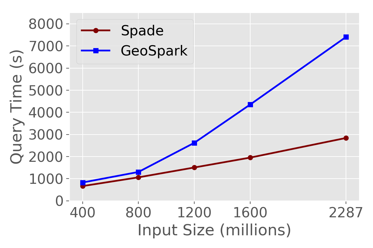
Figure 6: Scaling with input size (Twitter-Zip Code join).

In case of GeoSpark, we noticed that the running time of joins significantly increases once the data size (in terms of number of objects) becomes larger than a particular value. To confirm this, we executed the join query between subsets of Twitter data set with the Zip Code polygons. These subsets were extracted by increasing the time range of the tweets. Fig. 6 shows the results from this experiment. While the scaling is still linear, the slope however increases once the number of points grows beyond one billion. Therefore, to obtain the best timings for GeoSpark in our evaluation, we split the Twitter data into multiple smaller subsets (approximately 600M points each), and run the join on each subset. This resulted in over 2X speedup in the total running time when compared to executing a single join with the entire Twitter data. On the other hand, Spade scales better with increasing data sizes.

6.4 Distance-Based Queries

We evaluated the performance of Spade for distance-based joins. For this evaluation, we generated a random set of points within the spatial extent of the Taxi data and joined it with the Taxi data. Fig. 7(a) compares the performance of Spade, GeoSpark, and S2 when the size of the random points varies from 100 to 100K. We set the query distance to 20m for this experiment. Fig. 7(b) compares the performance of the three approaches when the size of point set is fixed at 100K, and the query distance is varied between 5m and 100m. S2 has the best performance for this class of queries, followed by Spade and GeoSpark respectively. This is because the S2 point index is optimized for distance-based queries.

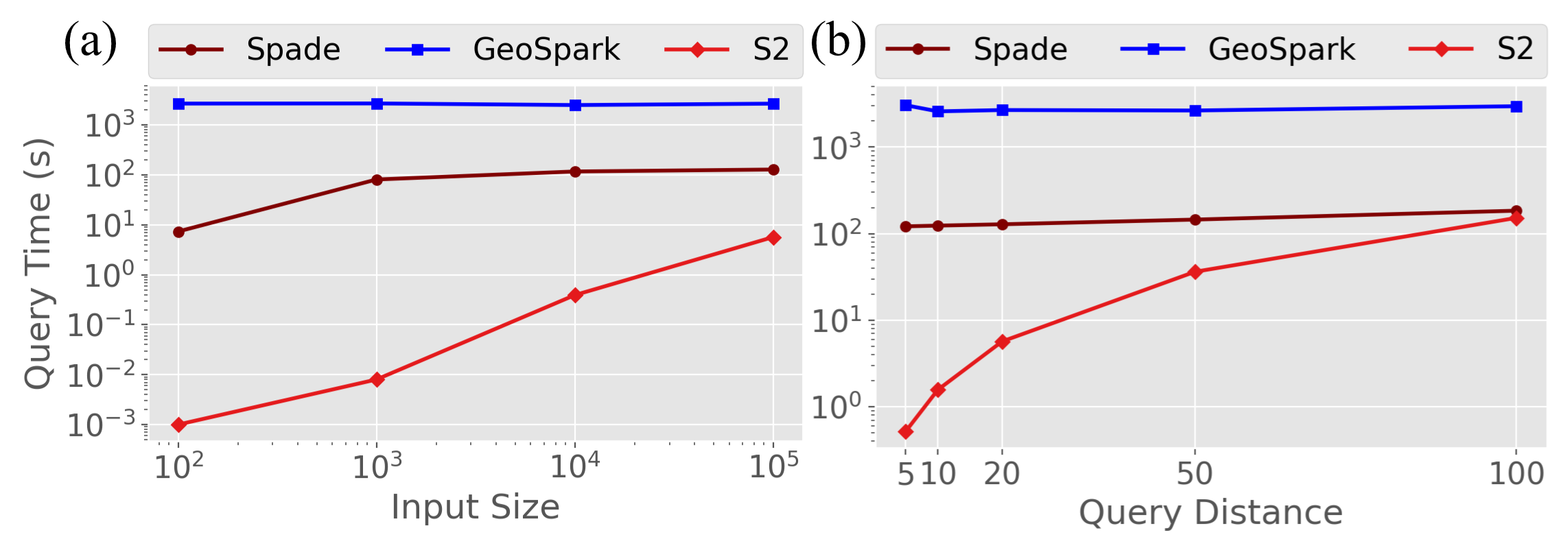
Figure 7: Performance of distance-based joins. (a) Varying number of points used with a constant query distance of 20 m. (b) Varying query distance for a join with 100K points.

Analysis and Discussion. In Fig. 7(a), we observe an interesting phenomenon with Spade: the query time for input size 100 is much faster than when the input size is 1000, after which the time stabilizes. This is because the number of intersections between the generated canvas polygons is much lower for 100 points compared to the other sizes, thus requiring considerably less processing. Otherwise, both Spade and GeoSpark have stable running times with varying parameters. On the other hand, S2’s time is dependent on the result size.

Note that, for this experiment, the input coordinates had to be converted into a meter-based projection system. As discussed earlier, this is performed in the shaders on the fly by Spade during query execution. While GeoSpark also supports this conversion, it took a significant amount of time ($>$ 2 hours). We therefore decided to pre-convert the coordinates, and used this in the experiments. In other words, the running times shown for GeoSpark do not reflect the time taken to convert the coordinates.

It is also interesting to note that running times using S2 increases with increasing query distance – as the distance increases, the running time of S2 becomes closer to that of Spade. This is due to the structure of the S2 index, where more index cells need to be covered for larger distances.

6.5 $k$NN Queries

We use the same set of generated points that was used in the evaluation of distance-based queries for $k$NN queries over the Taxi data.

Figure 8: Average time for 100 knn queries with varying k.

kNN Selection. Fig. 8 plots the average time taken for 100 $k$NN queries with the value of $k$ varying from 1 to 50. S2 takes just a few milliseconds to execute 100 queries and is significantly faster than Spade and GeoSpark. This is again because S2’s index is optimized to handle such queries.

kNN Join. Figs. 9(a) and 9(b) show the performance of Spade and S2 for varying sizes of the point data and different values of $k$, respectively. Similar to kNN select, S2 performs better than Spade for this query class. Given this significant performance difference, it will be interesting to investigate whether S2’s index can be adapted to be used with the GPU operators as well. Note that GeoSpark does not support $k$NN joins.

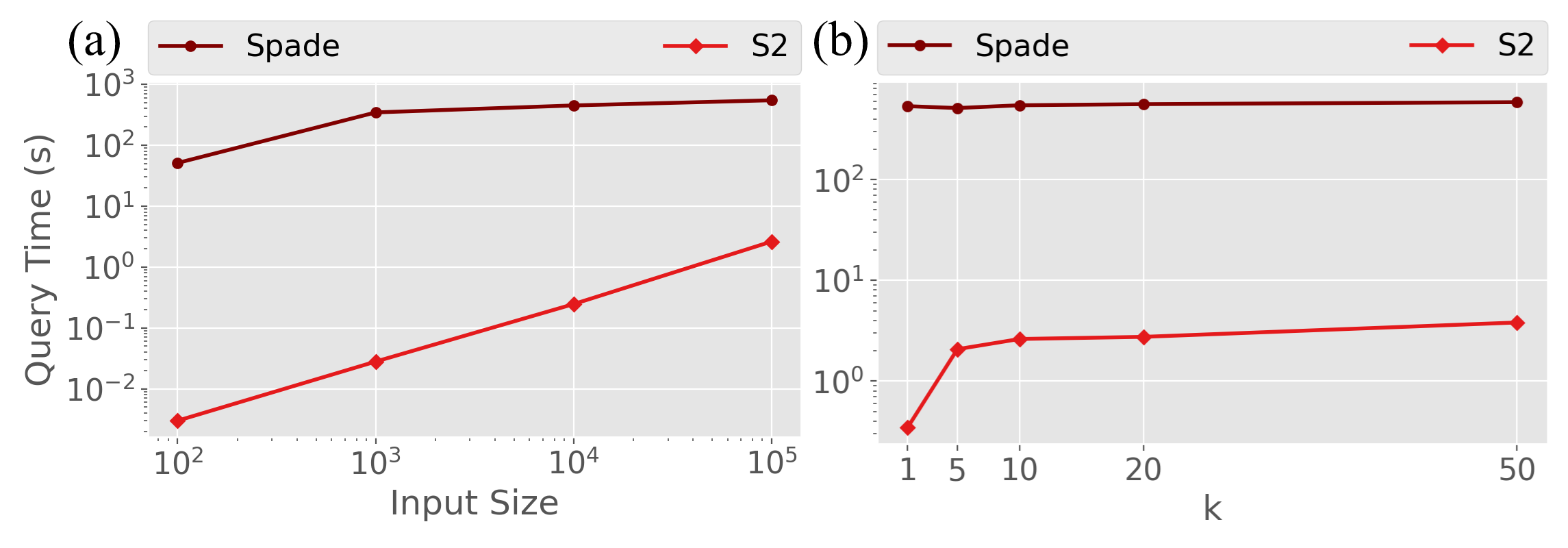
Figure 9: kNN joins. (a) Varying k. Point size = 100k. (b) Varying point size. k = 10.

6.6 Synthetic Data

In this section we evaluate the performance of selection and join queries on synthetically generated data. This evaluation allows us to test not only the scalability of Spade, but also its performance for different data distributions in a controlled manner.

Data sets and queries. The synthetic data was generated using the Spider spatial data generator [19]. We generated four classes of data sets comprising of points and rectangles. For each class, we generate 5 sizes as shown in Table 4. Note that the number of rectangles is chosen to have the same number of vertices as the point data sets.

1. Uniform Points: A collection of points uniformly distributed over a unit square.

2. Gaussian Points: A collection of points normally distributed over a unit square.

3. Uniform Boxes: A collection of axis parallel rectangles of varying sizes uniformly distributed over a unit square.

4. Gaussian Boxes: A collection of axis parallel rectangles of varying sizes normally distributed over a unit square.

Name	No. of Primitives (in millions)
Uniform Points	40, 80, 120, 160, 200
Gaussian Points	40, 80, 120, 160, 200
Uniform Boxes	10, 20, 30, 40, 50
Gaussian Boxes	10, 20, 30, 40, 50

Table 4: Synthetic data sets used in our evaluation.

For selection queries, we chose one of the polygons from the NYC Neighborhood data that was used in the Taxi experiments (Fig. 5(a)), centered it on the unit square, and scaled it to vary the extent of its bounding box in order to control the selectivity of the query. In particular, we vary the range such that the width (and height) of the bounding box of the polygon varies from 0.1 to 0.5 (i.e., covers half the width and height of the unit square) in increments of 0.1.

For join queries, we generated five parcel data sets having 1000, 2500, 5000, 7500, and 10000 parcels (non-intersecting rectangles of varying sizes) respectively.

Performance. Fig. 10 (left top) shows the running times of selection queries over the point data sets with varying selectivity. The running times are proportional to the selectivity. Queries over the Gaussian data takes more time than those over uniform data since they have a higher selectivity (Fig. 10 (bottom)). We would like to note that the index for both the uniform and Gaussian points were created using the same parameters. Thus, the cells of the grid index filtered in the index filtering stage is the same for a given query polygon for both the data sets. However, since the number of points within these cells is significantly more for the Gaussian data (more points are concentrated at the center of the unit square which is also the center of the query polygon), the data transfer time becomes higher. Thus, the above noticed time increase is mainly dominated by the I/O time, while the processing time on the GPU varies only by a few milliseconds.

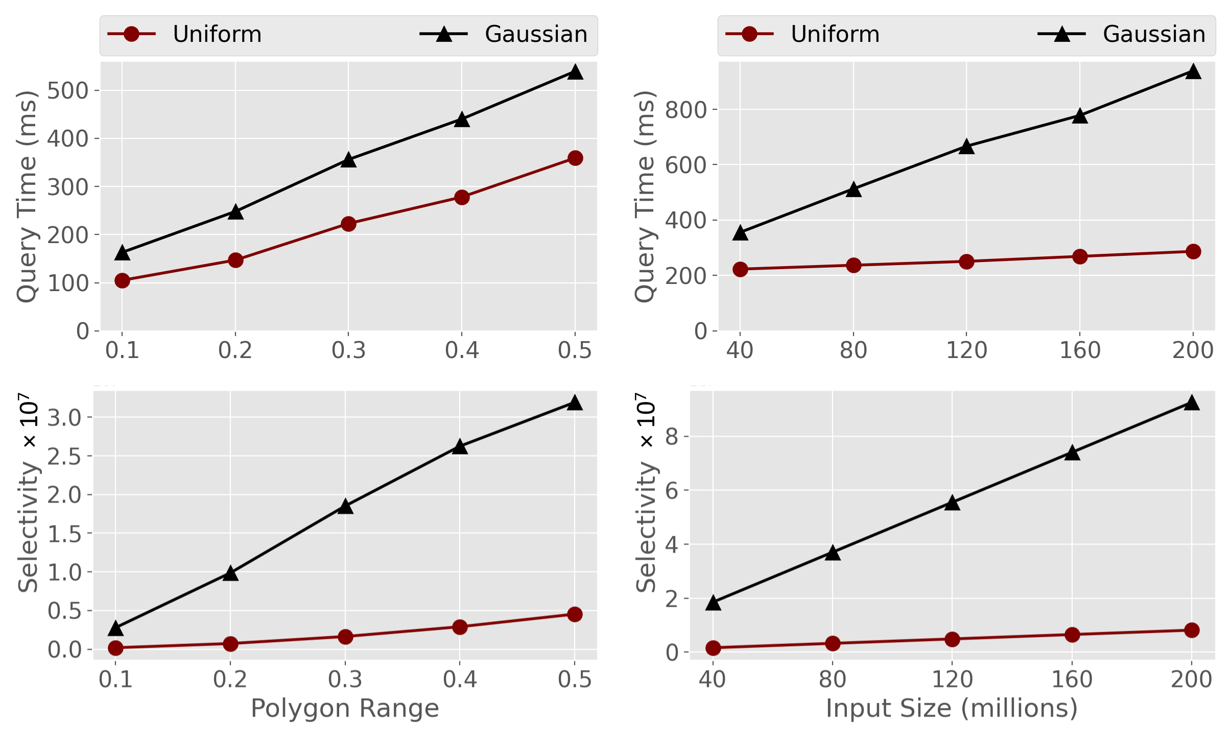
Figure 10: Selection over uniform and Gaussian point data. (Left Top) Varying the extent of the query polygon on the 40 million points data set. (Right Top) Varying the input data size. The range of the query polygon is fixed at 0.3. (Bottom) The selectivity of the queries corresponding to the top row.

Fig. 10 (right top) shows the running time when the query polygon is fixed and the input size is varied. As input size increases, the result size increases significantly for the Gaussian data when compared to the uniform data. This is reflected in the running times as well. Fig. 11 shows the performance of selections over polygonal data sets with varying selectivity (left) and varying input sizes (right). We see a trend similar to that of the point data.

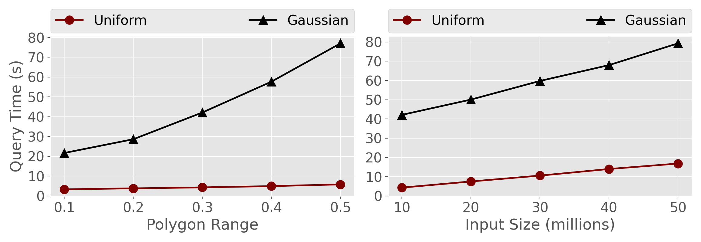
Figure 11: Selection over uniform and Gaussian box data. (Left) Varying the extent of the query polygon on the 10 million boxes data set. (Right) Varying the input data size. The range of the query polygon is fixed at 0.3.

Unlike the selection experiments on real data, we can control different aspects of the synthetic data. In particular, we can fix the complexity of the query polygon. Thus, we can see a clear trend of the running times scaling linearly with the query selectivity. On the other hand, it is difficult to see such trends using real data, especially in a spatial setting. This is because even when two query polygons have the same bounding box, they can have different selectivity due to their shape and complexity (e.g., a star query constraint vs. a square constraint, both with the same bounding box).

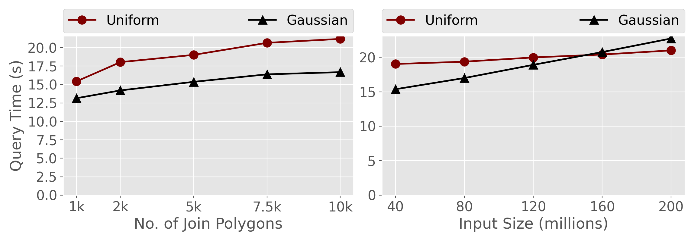
Figure 12: Performance of Point-Polygon joins. (Left) Varying the number of parcels in the join with the 40 million point data sets. (Right) Varying the size of the point data. Polygons with 5000 parcels was used for this join.

Fig. 12 shows the performance of point-polygon joins. Unlike the selection queries, the running time of joins over the Gaussian data is smaller than that over the uniform data. Recall that to execute joins, the filter phase first identifies all pairs of index grid cells that are then joined in a loop. Unlike the selection query, the join query used for this experiment is designed to cover the entire unit square. This requires the entire data to be transferred at least once to the GPU. However, since most of the points in the Gaussian data are concentrated at the center of the unit square, most of the query results are focused on a smaller set of grid cell pairs. Thus, larger amounts of contiguous data gets transferred into the GPU in a smaller set of rendering passes during the out-of-core processing. As a side-effect of this, when the GPU is processing (or rendering) a subset of the data, data that is to be processed next during the same (but larger) rendering pass gets transferred simultaneously in a pipelined fashion. On the other hand, in the join over uniform data, data transfers are spread uniformly across all the rendering passes, which we believe reduces the “pipeline” effect since the data transfer for the next rendering pass has to wait until the current rendering is complete. We believe this to be the primary reason for the shown trend where joins over Gaussian data is faster than that over uniform data. As input size increases, we however notice that this difference becomes smaller.

Figure 13: Performance of Polygon-Polygon joins. (Left) Varying the number of parcels in the join with the 10 million box data sets. (Right) Varying the size of the box data. Polygons with 5000 parcels was used for this join.

Fig. 13 shows the performance of polygon-polygon joins. We note that the above trend, where queries over Gaussian data are faster than those over uniform data, applies for this case as well.

7 Limitations and Discussions

Catering to the Long Tail. Spade is not a replacement to libraries such as S2 and systems such as GeoSpark – they can attain better performance and scalability in different scenarios. For example, since S2 is optimized for distance based queries, it can be faster than Spade for some queries. However, it requires large main memory hardware to run, while Spade can handle these queries on (commodity) systems with limited memory, albeit requiring a longer running time. Similarly, GeoSpark due to its distributed nature is better suited for efficiently executing batch-based queries over very large data sets which Spade may not be able to support. However, given that analysts making up the long tail often use commodity hardware for their processing, we believe that Spade would provide them with a viable alternative and thus democratize large scale spatial analytics.

Containment Queries. Spade currently supports intersection constraints for queries over line and polygonal data sets. Support for containment constraints can be added by simply treating each line (or polygon) as a collection of vertices, and testing for containment of this collection, i.e., point-based queries can be reused for this purpose. Note, however, that for points an intersection is equivalent to a containment test.

CPU-GPU hybrid execution. The currently supported queries (which are purely spatial) are such that it can be decomposed into a set of intersection tests and distance computations. This is not only amenable to parallelization, but can also efficiently make use of the graphics pipeline using the spatial algebra. Thus, we implemented these queries purely using the GPU. However, we believe that a hybrid approach will be beneficial when more complex queries are involved, possibly composed of both relational and spatial constraints. This also opens up new research problems to support dynamic scheduling and realization of query plans.

Improving I/O Performance. Even though I/O is a bottleneck in Spade’s execution times, the CPU-GPU bandwidth is continuously increasing through the introduction fast interconnects [21]. Therefore, advances in the hardware will naturally improve the performance of Spade. In addition to relying on technological advances, other strategies could also be used to further improve the I/O performance. For example, a pipeline-based approach could benefit GPUs with larger memory (such as desktop GPUs), wherein, while current batch is being executed in the GPU, the data from the next batch can be simultaneously loaded. Since CPU memory is in general much larger than the GPU memory, I/O can also be optimized by incorporating an appropriate caching policy that takes into account the order of operations. Recall that in spite of the memory bottlenecks, Spade already displayed very good performance. Therefore, we left these optimizations to be implemented in the next version of Spade.

Indexing Strategies and Tuning. Spade currently uses a grid-based indexing strategy, with the size of the grid cell being specified by the user. For our experiments, we used a general rule of thumb based on the GPU memory size for this purpose. Since, we focused on processing as much data as possible on the GPU (to maintain high GPU occupancy), this inadvertently also increased the amount of data filtered by the index. It will be interesting to explore automatic tuning based on system configuration and/or query workload.

Alternatively, other indexing strategies can also be used in a similar fashion. For example, if an R-tree based strategy is used, the bounding polygons of the R-tree leaves can be stored where the leaf sizes are adjusted similar to the grid cell size above. Note that, the index filtering, however, need not use the traditional R-tree traversal, and instead simply perform selections/joins on the bounding polygons.

Multi-GPU Support. While OpenGL provides an easy high level API for the graphics pipeline, its multi-GPU support is limited except in the case of Nvidia hardware and only under specific conditions (using an SLI interface or on Linux). In the next iteration of Spade, we intend to switch to use the recent Vulkan API [20] (which can be seen as an extension of OpenGL) that provides a much more fine-grained control over GPUs. This would also allow diverse GPUs (such as a discrete and an integrated GPU) to be used together, further improving performance even on laptops.

8 Related Work

The advent of hardware with multiple processing units has led to the design of new approaches that use them for spatial query processing. In particular, GPUs and multi-node clusters are extremely popular for this purpose.

Doraiswamy et al. [12] proposed a kd-tree based index optimized for GPUs to support interactive selections over point data. Zhang et al. [49, 51] used GPUs to join points with polygons. They index the points with a Quadtree to achieve load balancing and enable batch processing. They then extended their spatial join framework [52] to handle larger point data sets. However, to improve efficiency, they truncate coordinates to 16-bit integers, thus resulting in approximate joins. Tzirita Zacharatou et al. [41] proposed a rasterization-based approach to compute spatial aggregations between a set of points and polygons. Aghajarian et al. [2] proposed a GPU approach for both point-polygon and polygon-polygon joins. However, their approach only works on data that fits in GPU memory. Sainju et al. [36] proposed a grid-based join approach with the intent of mining co-located spatial events. Wang and others [45, 16, 6] proposed an approximate GPU-based join approach. There have also been GPU-based approaches for heatmap queries [47], creating and querying R-trees [34], and improving the filtering phase of spatial queries [39, 1]. All the above approaches use CUDA (except [39] and [41]), and are hence restricted to work only on Nvidia GPUs. While we reviewed a representative sample of GPU-based approaches, to the best of our knowledge, existing GPU-based spatial techniques are specific to a given query type.

OmniSci [29] provides a complete GPU-based SQL engine that also supports certain spatial queries. Similar to the above approaches, OmniSci is tied to Nvidia GPUs. Additionally, it is an in-memory system, and thus cannot be used to handle large data sets on commodity desktops and laptops.

An initial prototype for the algebra and canvas model was described in [10]. The prototype was developed as a proof of concept and it only supports spatial selection of points over data that fits in memory. Spade, in contrast, is a full-fledged query processing engine. As discussed above, we had to address several challenges to support the efficient evaluation of a rich set of spatial queries on commodity hardware.

Recently, several spatial database systems have been proposed using MapReduce such as Hadoop-GIS [3], Simba [46] and GeoSpark [48]. Eldawy and Mokbel [13] provide a comprehensive survey of these approaches. Pandey et al. [31] presented a detailed experimental evaluation of the state-of-the-art cluster-based spatial analytics systems. Pandey et al. [32] also evaluated common spatial libraries. As we discussed, these approaches are effective but out of reach for many analysts.

9 Conclusions

In this paper we presented Spade, a query engine that implements the recently proposed GPU-friendly spatial model and algebra [10] to support spatial queries over large data sets. Spade introduced two canvas-specific indexes to improve efficiency of spatial queries and a query optimizer to plan and execute queries on the GPU. We experimentally compared Spade with other approaches using large, real-world data sets. The results show that queries evaluated by Spade on a laptop with an Nvidia GPU have running times that are smaller or comparable to those of the cluster-based GeoSpark on a 17-node cluster, and of S2 running on a server with large memory. These results suggest that Spade has the potential to make large-scale spatial analytics within reach for a broad set of stakeholders. Since Spade was designed to use the relational schema to store spatial data sets, indexes, as well as the necessary meta-data, it can easily be integrated into existing relational database systems.

The novel approach to spatial query processing used by Spade not only opens new research opportunities in spatial query optimization and indexing, but also enables complex queries that were not possible before–e.g., accurate distance-based queries with respect to complex objects that are not supported in existing systems due to its complexity can be accomplished in Spade with a minimal overhead. Furthermore, with the recent Spark 3.x adding support for GPUs, we believe a significant performance boost can be obtained by integrating Spade with systems such as GeoSpark.

Acknowledgements

This work was partially supported by the DARPA D3M program and NSF award IIS-2106888. Any opinions, findings, and conclusions or recommendations expressed in this material are those of the authors and do not necessarily reflect the views of NSF and DARPA.

References

- [1] D. Aghajarian and S. K. Prasad. A spatial join algorithm based on a non-uniform grid technique over gpgpu. In Proceedings of the 25th ACM SIGSPATIAL International Conference on Advances in Geographic Information Systems, SIGSPATIAL ’17, New York, NY, USA, 2017. Association for Computing Machinery.
- [2] D. Aghajarian, S. Puri, and S. Prasad. Gcmf: An efficient end-to-end spatial join system over large polygonal datasets on gpgpu platform. In Proc. GIS, pages 18:1–18:10, New York, NY, USA, 2016. ACM.
- [3] A. Aji, F. Wang, H. Vo, R. Lee, Q. Liu, X. Zhang, and J. Saltz. Hadoop gis: A high performance spatial data warehousing system over mapreduce. PVLDB, 6(11):1009–1020, Aug. 2013.
- [4] N. Andrienko and G. Andrienko. Visual analytics of movement: An overview of methods, tools and procedures. Information Visualization, 12(1):3–24, Jan. 2013.
- [5] ArcGIS. https://www.arcgis.com, 2018.
- [6] F. Baig, C. Gao, D. Teng, J. Kong, and F. Wang. Accelerating spatial cross-matching on cpu-gpu hybrid platform with cuda and openacc. Frontiers in Big Data, 3:14, 2020.
- [7] T. Brinkhoff, H.-P. Kriegel, R. Schneider, and B. Seeger. Multi-step processing of spatial joins. In Proceedings of the 1994 ACM SIGMOD International Conference on Management of Data, SIGMOD ’94, page 197–208, New York, NY, USA, 1994. Association for Computing Machinery.
- [8] B. Bustos, O. Deussen, S. Hiller, and D. Keim. A graphics hardware accelerated algorithm for nearest neighbor search. In V. N. Alexandrov, G. D. van Albada, P. M. A. Sloot, and J. Dongarra, editors, Proc. ICCS, pages 196–199, Berlin, Heidelberg, 2006. Springer Berlin Heidelberg.
- [9] How-to: Tune Your Apache Spark Jobs. blog.cloudera.com/how-to-tune-your-apache-spark-jobs-part-2, 2021.
- [10] H. Doraiswamy and J. Freire. A gpu-friendly geometric data model and algebra for spatial queries. In Proceedings of the 2020 ACM SIGMOD International Conference on Management of Data, SIGMOD ’20, page 1875–1885, New York, NY, USA, 2020. Association for Computing Machinery.
- [11] H. Doraiswamy and J. Freire. A gpu-friendly geometric data model and algebra for spatial queries: Extended version, 2020.
- [12] H. Doraiswamy, H. T. Vo, C. T. Silva, and J. Freire. A gpu-based index to support interactive spatio-temporal queries over historical data. In Proc. ICDE, pages 1086–1097. IEEE, May 2016.
- [13] A. Eldawy and M. F. Mokbel. The era of big spatial data: A survey. Found. Trends databases, 6(3-4):163–273, Dec. 2016.
- [14] N. Ferreira, M. Lage, H. Doraiswamy, H. Vo, L. Wilson, H. Werner, M. Park, and C. Silva. Urbane: A 3d framework to support data driven decision making in urban development. In Proc. IEEE VAST 2015, pages 97–104, 2015.
- [15] N. Ferreira, J. Poco, H. T. Vo, J. Freire, and C. T. Silva. Visual exploration of big spatio-temporal urban data: A study of new york city taxi trips. IEEE TVCG, 19(12):2149–2158, 2013.
- [16] C. Gao, F. Baig, H. Vo, Y. Zhu, and F. Wang. Accelerating cross-matching operation of geospatial datasets using a cpu-gpu hybrid platform. In 2018 IEEE International Conference on Big Data (Big Data), pages 3402–3411, 2018.
- [17] S2 Geometry Library. https://github.com/google/s2geometry, 2021.
- [18] M. Harris, S. Sengupta, and J. D. Owens. Parallel prefix sum (scan) with CUDA. In GPU Gems 3, page 39. 2020.
- [19] P. Katiyar, T. Vu, A. Eldawy, S. Migliorini, and A. Belussi. Spiderweb: A spatial data generator on the web. In Proceedings of the 28th International Conference on Advances in Geographic Information Systems, SIGSPATIAL ’20, page 465–468, New York, NY, USA, 2020. Association for Computing Machinery.
- [20] Vulkan API. https://www.khronos.org/vulkan/, 2020.
- [21] C. Lutz, S. Breß, S. Zeuch, T. Rabl, and V. Markl. Pump up the volume: Processing large data on gpus with fast interconnects. In Proceedings of the 2020 ACM SIGMOD International Conference on Management of Data, SIGMOD ’20, page 1633–1649, New York, NY, USA, 2020. Association for Computing Machinery.
- [22] Mapbox. Earcut library. https://github.com/mapbox/earcut.hpp, 2020.
- [23] Metal Framework. https://developer.apple.com/documentation/metal, 2020.
- [24] Directx programming. https://docs.microsoft.com/en-us/windows/uwp/gaming/directx-programming, 2017.
- [25] New York City Taxi Data. https://www1.nyc.gov/site/tlc/about/tlc-trip-record-data.page, 2020.
- [26] Nvidia. CUDA C++ PROGRAMMING GUIDE, 2020.
- [27] 2010 Census Tracts. https://data.cityofnewyork.us/City-Government/2010-Census-Tracts/fxpq-c8ku, 2020.
- [28] Neighborhood Tabulation Areas. https://data.cityofnewyork.us/City-Government/Neighborhood-Tabulation-Areas-NTA-/cpf4-rkhq, 2020.
- [29] Open Source Analytical Database & SQL Engine. https://www.omnisci.com/platform/omniscidb, 2020.
- [30] OSM Zoom levels. https://wiki.openstreetmap.org/wiki/Zoom_levels, 2020.
- [31] V. Pandey, A. Kipf, T. Neumann, and A. Kemper. How good are modern spatial analytics systems? PVLDB, 11(11):1661–1673, July 2018.
- [32] V. Pandey, A. van Renen, A. Kipf, and A. Kemper. How good are modern spatial libraries? Data Science and Engineering, (2):1–17, Nov. 2020.
- [33] M. Pavlovic, T. Heinis, F. Tauheed, P. Karras, and A. Ailamaki. Transformers: Robust spatial joins on non-uniform data distributions. In Proc. ICDE, pages 673–684. IEEE, May 2016.
- [34] S. K. Prasad, M. McDermott, X. He, and S. Puri. Gpu-based parallel r-tree construction and querying. In 2015 IEEE International Parallel and Distributed Processing Symposium Workshop, pages 618–627, 2015.
- [35] M. Raasveldt and H. Mühleisen. Monetdblite: An embedded analytical database. CoRR, abs/1805.08520, 2018.
- [36] A. M. Sainju, D. Aghajarian, Z. Jiang, and S. Prasad. Parallel grid-based colocation mining algorithms on gpus for big spatial event data. IEEE Transactions on Big Data, 6(1):107–118, 2020.
- [37] D. Shreiner, G. Sellers, J. M. Kessenich, and B. M. Licea-Kane. OpenGL Programming Guide: The Official Guide to Learning OpenGL, Version 4.3. Addison-Wesley Professional, 8th edition, 2013.
- [38] STIG Standalone Code. https://github.com/harishd10/mongodb/tree/master/standalone", 2021.
- [39] C. Sun, D. Agrawal, and A. El Abbadi. Hardware acceleration for spatial selections and joins. In Proceedings of the 2003 ACM SIGMOD International Conference on Management of Data, SIGMOD ’03, page 455–466, New York, NY, USA, 2003. Association for Computing Machinery.
- [40] Tableau Software. https://www.tableau.com/, 2020.
- [41] E. Tzirita Zacharatou, H. Doraiswamy, A. Ailamaki, C. T. Silva, and J. Freire. Gpu rasterization for real-time spatial aggregation over arbitrary polygons. PVLDB, 11(3):352–365, 2017.
- [42] World Countries. https://hub.arcgis.com/datasets/a21fdb46d23e4ef896f31475217cbb08\_1, 2020.
- [43] U.S. County Shapefile. https://catalog.data.gov/dataset/tiger-line-shapefile-2017-nation-u-s-current-county-and-equivalent-national-shapefile, 2020.
- [44] U.S. Zip Code Tabulation Area. https://catalog.data.gov/dataset/tiger-line-shapefile-2019-2010-nation-u-s-2010-census-5-digit-zip-code-tabulation-area-zcta5-na, 2020.
- [45] K. Wang, Y. Huai, R. Lee, F. Wang, X. F. Zhang, and J. Saltz. Accelerating pathology image data cross-comparison on cpu-gpu hybrid systems. Proceedings of the VLDB Endowment International Conference on Very Large Data Bases, 5:1543–1554, 07 2012.
- [46] D. Xie, F. Li, B. Yao, G. Li, L. Zhou, and M. Guo. Simba: Efficient in-memory spatial analytics. In Proc. SIGMOD, pages 1071–1085, New York, NY, USA, 2016. ACM.
- [47] K. K. Yong, W. K. Ho, M. W. Chua, and S. See. A gpu query accelerator for geospatial coordinates computation. In 2015 International Conference on Cloud Computing Research and Innovation (ICCCRI), pages 166–172, 2015.
- [48] J. Yu, Z. Zhang, and M. Elsayed. Spatial data management in apache spark: the geospark perspective and beyond. GeoInformatica, 23(1):37–78, Jan. 2018.
- [49] J. Zhang and S. You. Speeding up large-scale point-in-polygon test based spatial join on gpus. In Proc. BigSpatial, pages 23–32, 2012.
- [50] J. Zhang, S. You, and L. Gruenwald. High-performance online spatial and temporal aggregations on multi-core cpus and many-core gpus. In Proc. DOLAP, pages 89–96, 2012.
- [51] J. Zhang, S. You, and L. Gruenwald. High-performance spatial join processing on gpgpus with applications to large-scale taxi trip data. Technical report, The City College of New York, 2012.
- [52] J. Zhang, S. You, and L. Gruenwald. Efficient parallel zonal statistics on large-scale global biodiversity data on gpus. In Proc. BigSpatial, pages 35–44, New York, NY, USA, 2015. ACM.