Online Meta-Learning For Hybrid Model-Based Deep Receivers

Abstract

Recent years have witnessed growing interest in the application of deep neural networks (DNNs) for receiver design, which can potentially be applied in complex environments without relying on knowledge of the channel model. However, the dynamic nature of communication channels often leads to rapid distribution shifts, which may require periodically retraining. This paper formulates a data-efficient two-stage training method that facilitates rapid online adaptation. Our training mechanism uses a predictive meta-learning scheme to train rapidly from data corresponding to both current and past channel realizations. Our method is applicable to any deep neural network (DNN)-based receiver, and does not require transmission of new pilot data for training. To illustrate the proposed approach, we study DNN-aided receivers that utilize an interpretable model-based architecture, and introduce a modular training strategy based on predictive meta-learning. We demonstrate our techniques in simulations on a synthetic linear channel, a synthetic non-linear channel, and a COST 2100 channel. Our results demonstrate that the proposed online training scheme allows receivers to outperform previous techniques based on self-supervision and joint-learning by a margin of up to 2.5 dB in coded bit error rate in rapidly-varying scenarios.

I Introduction

Deep learning systems have demonstrated unprecedented success in various applications, ranging from computer vision to natural language processing, and recently also in physical layer applications. While traditional receiver algorithms are channel-model-based, relying on mathematical modeling [2] of the signal transmission, propagation, and reception. DNN-based receivers have the potential to operate efficiently in model-deficient scenarios where the channel model is unknown, highly complex [3, 4], or difficult to optimize for [5, 6]. Generally, deep learning can be integrated with receiver design either by using conventional black-box DNN architectures trained end-to-end; or by leveraging model-based solutions [7, 8, 9, 10], whereby specific blocks of a receiver’s architecture are replaced by neural networks, e.g., via deep unfolding [8]. Contrary to black-box receivers, which make limited assumptions on the data distribution, model-based deep receivers exploit additional domain knowledge, in the form of a specific receiver structure that is tailored to the channel of interest.

Channel encoding and decoding can be optimized jointly end-to-end as in [11, 12, 13], or decoding can be separately trained as studied in [14, 15, 16, 17]. Classical channel estimation can be enhanced as compared to the existing compressive sensing-based methods [18, 19] via the integration with DNNs. DNN-aided receiver designs are shown to outperform classical methods in non-linear environments in [20, 21, 22, 23, 24]. In the areas of optical fiber communication and underwater acoustics, in which non-linearity dominates, DNN-aided solutions have also proved useful [25, 26, 27, 28, 29]. Additional applications of DNN-aided receivers include detection by reconfigurable intelligent surface (RIS) and blind reception with multiple modulation and coding schemes [30, 31].

Despite their potential in implementing digital receivers [32, 33], deep learning solutions are subject to several challenges that limit their applicability in important communication scenarios. A fundamental difference between digital communications and traditional deep learning applications stems from the dynamic nature of wireless channels. DNNs consist of highly-parameterized models that can represent a broad range of mappings. As such, massive data sets are typically required to obtain a desirable mapping. The dynamic nature of communication channels implies that a DNN trained for a given channel may no longer perform well on future channel realizations. While one can possibly enrich data sets via data augmentation [34, 35, 36] or robustify a DNN so that it copes with multiple channel realizations via Bayesian learning [37, 38], a DNN-aided receiver is still likely to have to adapt at some point when operating in time-varying conditions.

To apply DNN-based transceivers in time-varying channels, two main approaches are considered in the literature. The first attempts to learn a single mapping that is applicable to a broad range of channel conditions. This class of methods includes the approach of training a DNN using data corresponding to an extensive set of expected channel conditions, which is referred to as joint learning[23, 39]. An additional, related, method trains in advance a different network for each expected channel, and combines them as a deep ensemble [40]. However, these strategies typically require a large amounts of training data, and deviating from the training setup, i.e., operating in a channel whose characteristics differ from those observed during training, can greatly impair performance [41].

An alternative strategy is to track the channel variations. This can be achieved by providing the DNN with a model-based channel estimate [42, 43, 44, 45, 46]. However, channel estimation involves imposing a relatively simple model on the channel, such as a linear Gaussian models, which may be inaccurate in some setups. When operating without channel knowledge, tracking the channel involves periodically retraining the network. To provide data for retraining, one must either transmit frequent pilots, or, alternatively, use decoded data for training with some forward error correction (FEC) scheme. Specifically, the mechanism employed in [47, 48, 49] re-encodes the decoded bits, and then it computes the Hamming distance between the re-encoded bits and the hard-decision obtained from the channel observations. If this difference (normalized to the block length) is smaller than some threshold value, the decoded bits are considered to be reliable and are used for retraining. Another approach is to further encode the block with error detection codes such as cyclic redundancy check (CRC), which identifies decoding errors. If the received block is deemed to be detected correctly, as indicated by the above measures, it is fed back into the DNN-aided receiver, with the predicted symbols as the training labels. This process implements a form of self-supervised training as defined in [50, 51, 52].

Data-driven implementations of the Viterbi scheme [53], BCJR method [54], and iterative soft interference cancellation (SIC) [55] were proposed in [47, 56, 57], respectively. Yet, even with model-based architectures, relatively large data sets are still required and typical DNN training procedures are likely to induce non-negligible delay. The ability to retrain quickly is highly dependent on the selection of a suitable initialization of the iterative training algorithm. While the common strategy is to use random weights, the work [47] used the previous learned weights as an initial point for retraining. An alternative approach is to optimize the initial point via meta-learning [58, 59, 60, 41, 61]. Following this method, one not only retrains, but it also optimizes the hyperparameters that define the retraining process. Meta-learning was adopted to facilitate prediction of blockages [62], beam tracking [63], and power control [64].

For DNN-aided receivers, it was shown in [41] that by optimizing the initial weights via meta-learning, the receiver can quickly adapt to varying channel conditions. The method proposed in [41] is designed for settings where in each coherence duration, the transmitters send pilots followed by data packets, such that the receiver can train using the pilots and then apply its DNN to the received data. This technique does not naturally extend to rapidly time-varying channels. In fact, in such cases, the channel can change between the packets and thus a receiver trained with the pilots may no longer be suitable for detecting the following information messages.

In this work we propose an online training algorithm to enable rapid adaptation of DNN-based receivers via meta-learning. Our algorithm considers both long and short term variations in the channel: We choose the initial weights of the deep receiver via meta-learning [65], while tracking local variations in a decision-directed self-supervised manner [47, 48]. While meta-learning in [41] is designed to train from pilots corresponding to the same channel over which the information blocks are transmitted, we consider rapidly time-varying channels, where each block undergoes a different channel realization. Consequently, while [41] was able to build upon the conventional model-agnostic meta-learning (MAML) algorithm [65], our proposed approach modifies MAML to incorporate predictions of channel realizations in future blocks.

To further facilitate efficient adaptation to changing conditions, we instantiate the proposed meta-learning approach for settings in which the DNN-aided receiver employs an interpretable model-based deep architecture [8]. Hybrid design techniques, such as deep unfolding [66], neural augmentation [67], and DNN-based algorithms [68], have given rise to a multitude of deep receiver architectures, including, e.g., [56, 45, 42, 14, 22, 16, 57, 47]. These hybrid model-based/data-driven deep receivers are generally more compact in terms of number of parameters, requiring fewer training samples to reach convergence [8]. We propose to exploit the structure of model-based deep receivers in order to efficiently re-train only specific modules of the architecture with the aid of meta-learning [69]. This new approach to online training, referred to as modular training, further reduces the overall error rate over rapidly-changing scenarios.

Our main contributions are summarized as follows:

• Predictive online meta-learning algorithm: We introduce a meta-learning strategy that is applicable to any DNN-based receiver. The proposed approach integrates MAML [65] with the prediction of time-varying channels to ensure that a small number of gradient updates can efficiently minimize the loss (or error) on the next data block.

• Modular training of interpretable architectures: We instantiate the proposed meta-learning approach for hybrid model-based/data-driven deep receivers that leverage the structure of multipath channels. We propose to only retrain specific modules of the receiver architecture that need adaptation due to temporal variations of the channel. Fast and efficient adaptation of the machine learning modules utilize a variant of MAML referred to as almost-no-inner-loop (ANIL) [69], which incorporates a priori information about channel variability.

• Extensive Experimentation: We extensively evaluate the proposed training scheme for both single-input single-output (SISO) and multiple-input multiple-output (MIMO) systems, considering three different time-varying channel profiles: linear synthetic channel, a non-linear synthetic channel, and a COST 2100 [70] channel. We show gains of up to 2.5 dB in coded bit error rate (BER), compared to joint and online approaches, over a set of challenging channels. Compared to previous approaches for handling time-varying channels without relying on pilots, such as self-supervision [47] and joint learning [39], we show that the proposed techniques offer advantages in terms of average symbol error rate (SER), while reducing the pilot overhead.

The rest of this paper is organized as follows: Section II details the system model, while Section III presents the meta-learning algorithm. In Section IV we focus on model-based deep receivers and show how to exploit their interpretable structure via modular training. Finally, experimental results and concluding remarks are detailed in Section V and Section VI, respectively.

Throughout the paper, we use boldface letters for vectors, e.g., ${{\boldsymbol{x}}}$; $({{\boldsymbol{x}}})_{i}$ denotes the $i$th element of ${{\boldsymbol{x}}}$. Calligraphic letters, such as $\mathcal{X}$, are used for sets, and $\mathcal{R}$ is the set of real numbers.

II System Model

In the section, we describe the system model in Subsection II-A, and then formulate the design problem in Subsection II-B.

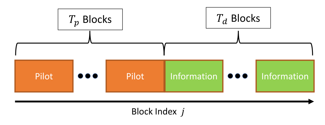
Figure 1: Transmission model. The channel is constant in each block and changes across blocks.

II-A Channel Model

We consider communication over casual finite-memory block-wise varying channels with multiple users. The channel output depends on the last $L>0$ transmitted symbols, where $L$ is the memory length. The channel is constant within a block of $B$ channel uses, which corresponds to the coherence duration of the channel.

Let ${\boldsymbol{S}}_{i,j}\in\mathcal{S}^{K}$ be the $K$ symbols transmitted from constellation $\mathcal{S}$ at the $i$th time instance, $i\in\{1,2,\ldots,B\}:=\mathcal{B}$, of the $j$th block. Here, the constellation size is $|\mathcal{S}|$, and $K$ denotes the number of users transmitting simultaneously. Accordingly, when $K>1$, the setting represents a multiple access channel, while $K=1$ corresponds to point-to-point communications. The channel output is denoted by ${{\boldsymbol{Y}}}_{i,j}\in\mathcal{Y}^{N}$, where $N$ represents the number of receive antennas, and is given by a stochastic function of the last $L$ transmitted symbols $\bar{{{\boldsymbol{S}}}}_{i,j}:=[{\boldsymbol{S}}_{i-L+1,j},\ldots,{\boldsymbol{S}}_{i,j}]^{T}$. Specifically, by defining the $j$th transmitted block as ${{\boldsymbol{S}}}_{j}:=\{{\boldsymbol{S}}_{i,j}\}_{i\in\mathcal{B}}$ and its corresponding observations as ${{\boldsymbol{Y}}}_{j}:=\{{{\boldsymbol{Y}}}_{i,j}\}_{i\in\mathcal{B}}$, the conditional distribution of the channel output given its input satisfies

$$P_{{{\boldsymbol{Y}}}_{j}|{{\boldsymbol{S}}}_{j}}\left({\boldsymbol{y}}_{j}|{\boldsymbol{s}}_{j}\right)=\prod\limits_{i\!=\!1}^{B}P_{{{\boldsymbol{Y}}}_{i,j}|\bar{{{\boldsymbol{S}}}}_{i,j}}\left({\boldsymbol{y}}_{i,j}|\bar{{{\boldsymbol{s}}}}_{i,j}\right).$$ (1)

In (1), the lower-case notations ${\boldsymbol{s}}_{j}$, ${\boldsymbol{y}}_{i,j}$, and $\bar{{\boldsymbol{s}}}_{i,j}$ represent the realizations of the random variables ${{\boldsymbol{S}}}_{j}$, ${{\boldsymbol{Y}}}_{i,j}$, and $\bar{{{\boldsymbol{S}}}}_{i,j}$, respectively. We set ${\boldsymbol{S}}_{i,j}\equiv{\boldsymbol{0}}$ for $i<0$, i.e., we assume a guard interval of at least $L-1$ time instances between blocks.

The input-output relationship in (1) describes a generic, possibly multi-user, channel model with block-wise temporal variations. These channel variations, i.e., changes between different values of the block index $j$, can often be attributed to some phenomena, e.g. a movement of one or several of the communicating entities. We do not impose a specific model on the channel observed in each block, representing it by the generic conditional distribution in (1), which can take a complex and possibly intractable form. Two important special cases include:

1. SISO Finite-Memory Channels: The first type of channels considered in this work is the multipath SISO case; that is, we set $N=K=1$.

2. Flat MIMO Channels: Another channel of interest is the memoryless ($L=1$) MIMO channel, where $N>1$ and $K>1$. Such settings specialize multi-user uplink MIMO systems, where $K$ is the number of single-antenna transmitters.

We consider the scenario illustrated in Fig. 1, where a total of $T_{p}$ pilot blocks and $T_{d}$ information blocks are transmitted sequentially. That is, blocks indexed $j\in\{0,\ldots,T_{p}-1\}$ are known pilots, transmitted in the training phase, while $j\in\{T_{p},\ldots,T_{p}+T_{d}-1\}$ are information blocks that compose the test phase. The pilot blocks convey a known message, whereas the information blocks are unknown and are utilized to test the proposed schemes. Each information block, i.e., ${\boldsymbol{S}}_{j}$ for $j\in\{T_{p},\ldots,T_{p}+T_{d}-1\}$, is encoded into a total of $B$ symbols using both FEC coding and error detection codes. Error detection codes, such as cyclic redundancy check, allow the receiver to identify the presence of errors in the decoding procedure.

II-B Problem Formulation

We consider the problem of symbol detection in the generic channel model formulated in Subsection II-A. The fact that we do not impose a specific model of the channel, allowing its input-output relationship to take complex forms in each block, combined with the availability of data based on the protocol detailed above, motivate using DNN-based receivers. The core challenge in applying DNN-based receivers for the considered channel stems from its temporal variations. Our objective is thus to derive a training algorithm that aids DNN-based receivers in recovering the transmitted data from the channel outputs $\{{\boldsymbol{Y}}_{j}\}_{j=T_{p}}^{T_{p}+T_{d}-1}$. The DNN-based receiver trains on the pilot blocks, and is tested on the transmitted information blocks.

Let ${\boldsymbol{\varphi}}$ denote the parameters of the DNN-based receiver, i.e., the weights of the neural network. These parameters dictate the receiver mapping, which, for a given ${\boldsymbol{\varphi}}$, is denoted by $\hat{{\boldsymbol{s}}}(\cdot;{\boldsymbol{\varphi}}):\mathcal{Y}^{N\times B}\mapsto\mathcal{S}^{K\times B}$, i.e., $\hat{{\boldsymbol{s}}}({\boldsymbol{y}};{\boldsymbol{\varphi}})$ denotes the symbol block recovered by the receiver parameterized with ${\boldsymbol{\varphi}}$ when applied to the channel output block ${\boldsymbol{y}}$. By using the abbreviated symbol $\hat{{\boldsymbol{s}}}_{j}({\boldsymbol{\varphi}})$ to denote the symbols detected based on the channel output of the $j$th block, with $\hat{{\boldsymbol{s}}}_{i,j}({\boldsymbol{\varphi}})\in\mathcal{S}^{K}$ being its $i$th symbol, $i\in\mathcal{B}$, our goal is to propose an algorithm that allows a DNN-based receiver to continuously provide low error rates over the data blocks:

$$\mathop{\min}_{{\boldsymbol{\varphi}}_{j}}\Big{(}\frac{1}{B}\sum_{i=1}^{B}\Pr\left(\hat{{\boldsymbol{s}}}_{i,j}({\boldsymbol{\varphi}}_{j})\neq{\boldsymbol{s}}_{i,j}\right)\Big{)},\qquad j\in\{T_{p},\ldots,T_{p}+T_{d}-1\}.$$ (2)

The parameter vector ${\boldsymbol{\varphi}}$ in (2) is allowed to change between blocks, namely, the DNN-based receiver can adapt its parameters over time, while the pilot blocks are utilized to initialize ${\boldsymbol{\varphi}}$.

As our problem formulation does not impose a specific structure on the DNN-based receiver, we first consider online adaptation that is agnostic of the receiver structure. This approach integrates channel predictions into the adaptation of the receiver’s parameters. Next, we show how one can employ the modular architecture of model-based deep receivers to further reduce the error rate over the transmitted data blocks, facilitating coping with rapid variations and a short coherence duration.

III Predictive Online Meta-Learning for DNN-Based Receivers

In this section we study parameter adaptation of a generic DNN-based receiver to continuously maintain low error rates in time-varying channels. Modification of these weights involves training, which requires the receiver to obtain recent examples of pairs of transmitted blocks and corresponding observed channel outputs. This gives rise to two core challenges. First, while one can use pilots, the time-varying nature of the channel implies that pilot-based examples are likely to not represent the channel conditions for some or all of the data blocks. In addition, even if one can extract labeled training data from blocks containing information messages, when the channel varies quickly, the amount of data from the instantaneous channel may be limited. We draw inspiration from the successful applications of meta-learning for facilitating training from pilots corresponding to the current channel conditions [41], as well as the emergence of FEC-based self-supervision for pilot-free online training [47].

To describe this algorithm, we begin by introducing self-supervised training in Subsection III-A for slow-fading channels. Then we extend online training to rapidly time-varying channels in Subsection III-B, which presents our training method. The resulting algorithm is detailed in Subsection III-C.

III-A Self-Supervised Online Training

The first part of our online adaptation mechanism is based on self-supervision, which extracts training data from information-bearing blocks. The approach follows [47] by re-using confident decisions via the re-encoding of a successfully decoded word for use in online training.

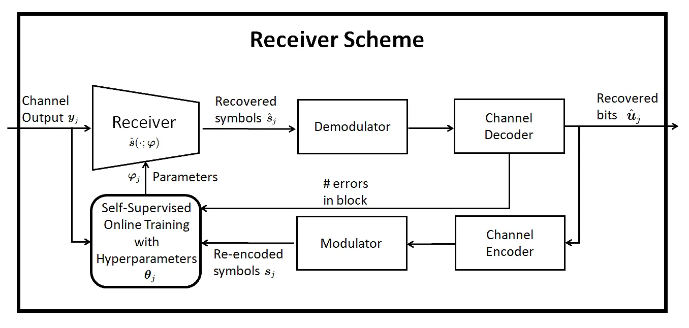
Figure 2: Self-supervised online training based on channel coding.

First, we initialize the parameter vector ${\boldsymbol{\varphi}}_{T_{p}}$ by training over the obtained $T_{p}$ pilot blocks. Then, for each information block $j\in\{T_{p},\ldots,T_{p}+T_{d}-1\}$, when decoding is reported by the decoder to be correct, the re-encoded data pair $\{{\boldsymbol{s}}_{j},{\boldsymbol{y}}_{j}\}$ is used as training data to update the parameters for the next block, i.e., to generate ${\boldsymbol{\varphi}}_{j+1}$. The same training is applied to the receiver during pilots and information blocks transmission. Since symbol detection can be treated a classification task, this is achieved by minimizing the empirical cross entropy loss as

$$\mathop{\arg\min}_{{\boldsymbol{\varphi}}}\left\{\mathcal{L}_{j}({\boldsymbol{\varphi}})=-\sum_{i=1}^{B}\log\hat{P}_{{\boldsymbol{\varphi}}}\left({\boldsymbol{y}}_{i,j}|\bar{{\boldsymbol{s}}}_{i,j}\right)\right\}.$$ (3)

In (3), the probability $\hat{P}_{{\boldsymbol{\varphi}}}\left({\boldsymbol{y}}|\bar{{\boldsymbol{s}}}\right)$ is the soft output of the DNN-based receiver corresponding to $\bar{{\boldsymbol{s}}}$ when applied to the data block ${\boldsymbol{y}}$. The optimization problem in (3) is approximately solved using gradient-based optimization with some learning rate $\eta$, i.e., via $I_{\rm sgd}$ iterations of the form

$${\boldsymbol{\varphi}}_{j+1}^{(t+1)}={\boldsymbol{\varphi}}_{j+1}^{(t)}-\eta\nabla_{{\boldsymbol{\varphi}}_{j+1}^{(t)}}\mathcal{L}_{j}({\boldsymbol{\varphi}}_{j+1}^{(t)}).$$ (4)

The computation of the gradient steps requires an initialization ${\boldsymbol{\varphi}}_{j+1}^{(0)}$, which is a hyperparameter of the training procedure. We henceforth denote this hyperparameter vector used for self-supervised training of ${\boldsymbol{\varphi}}_{j+1}$ as ${\boldsymbol{\theta}}_{j+1}$, i.e., ${\boldsymbol{\varphi}}_{j+1}^{(0)}={\boldsymbol{\theta}}_{j+1}$. The gradient in (4) is typically approximated via random sampling among available $B$ symbols within the block to implement stochastic gradient descent (SGD) and its variants, typically used for training DNNs [71, Ch. 4]. The online training scheme is presented in Fig. 2. The self-supervision training algorithm is based on the assumption that channel conditions vary smoothly across blocks, so that a receiver trained on data from the $j$th block is likely to correctly detect data also from the $(j+1)$th channel realization. Following this line of reasoning, [47] used ${\boldsymbol{\theta}}_{j+1}={\boldsymbol{\varphi}}_{j}$.

However, this assumption is inadequate for tracking fast-varying channels. Adapting locally in a self-supervised manner by setting the hyperparameter ${\boldsymbol{\theta}}_{j+1}={\boldsymbol{\varphi}}_{j}$ accounts for only short term variations, as both the data and the optimization hyperparameters correspond to the current instantaneous channel realization. In order to train effectively from short blocks in complex channels, we propose to incorporate long term relations by altering the setting of the hyperparameter ${\boldsymbol{\theta}}_{j+1}$ via meta-learning.

III-B Predictive Online Meta-Learning

Figure 3: Illustration of the operation of the proposed meta-training algorithm in test phase.

To this end, following the MAML framework [65], we define the support task as the detection of the current block; while the query task, for which the parameters should adapt, is the detection of the next block. Upon the reception of a block of channel outputs ${\boldsymbol{y}}_{j}$, the method operates in three stages, illustrated as a block diagram in Fig. 3:

1. Detection: Each incoming data block ${\boldsymbol{y}}_{j}$ is mapped into an estimated symbol block $\hat{{\boldsymbol{s}}}_{j}$, with the mapping determined by the current parameters vector ${\boldsymbol{\varphi}}_{j}$. Then, it is decoded by using an FEC decoder to produce the demodulated and decoded message $\hat{{\boldsymbol{u}}}_{j}$. When decoding is correct, as determined by error detection, the message $\hat{{\boldsymbol{u}}}_{j}$ is re-encoded and modulated, producing an estimated transmitted vector $\tilde{{\boldsymbol{s}}}_{j}$ (see Section III-A). This block is inserted along with its observations ${\boldsymbol{y}}_{j}$ into a labelled buffer $\mathcal{D}_{j}$. This buffer contains pairs of previously received blocks ${\boldsymbol{y}}_{j}$ along with their corresponding transmitted signal ${\boldsymbol{s}}_{j}$, or an estimated version thereof. The buffer $\mathcal{D}_{j}$ contains $D$ such pairs, and is managed in a first-in-first-out mode. A pilot block $({\boldsymbol{s}}_{j},{\boldsymbol{y}}_{j})$ is directly inserted into $\mathcal{D}_{j}$ upon reception.

2. Online training: In each data block $j$, if decoding is successful, the weights ${\boldsymbol{\varphi}}_{j+1}$ are updated by using the hyperparameters ${\boldsymbol{\theta}}_{j+1}$ and the newly decoded block $({\boldsymbol{s}}_{j},{\boldsymbol{y}}_{j})$, as detailed in Subsection III-A. Otherwise, no update is carried out. A similar update takes place for pilot block $j$ with pilot block $({\boldsymbol{s}}_{j},{\boldsymbol{y}}_{j})$. This update is the same as in [47].

3. Meta-learning: The hyperparameter ${\boldsymbol{\theta}}_{j+1}$ is optimized to enable fast and efficient adaptation of the model parameter ${\boldsymbol{\varphi}}_{j+1}$ based on the last successfully decoded block $({\boldsymbol{s}}_{j},{{\boldsymbol{y}}}_{j})$ using (4). Adopting MAML [65], we leverage the data in the buffer $\mathcal{D}_{j}$ by considering the problem

   $${\boldsymbol{\theta}}_{j+1}=\mathop{\arg\min}\limits_{{\boldsymbol{\theta}}}\sum\limits_{\{({\boldsymbol{s}}_{j^{\prime}},{{\boldsymbol{y}}}_{j^{\prime}}),({\boldsymbol{s}}_{j^{\prime}+1},{{\boldsymbol{y}}}_{j^{\prime}+1})\}\in\mathcal{D}_{j}}\mathcal{L}_{j^{\prime}+1}({\boldsymbol{\varphi}}={\boldsymbol{\theta}}-\kappa\nabla_{{\boldsymbol{\theta}}}\mathcal{L}_{j^{\prime}}({\boldsymbol{\theta}})),$$ (5)

   where $\kappa>0$ is the meta-learning rate. The parameters ${\boldsymbol{\varphi}}$ in (5) follow the same update rule in (4) by using the last available block $({\boldsymbol{s}}_{j^{\prime}},{\boldsymbol{y}}_{j^{\prime}})$ in the buffer prior to index $j^{\prime}+1$. Furthermore, in line with (3), the loss $\mathcal{L}_{j^{\prime}+1}({\boldsymbol{\varphi}})$ is computed based on data from the following available block $({\boldsymbol{s}}_{j^{\prime}+1},{\boldsymbol{y}}_{j^{\prime}+1})$. When the buffer $\mathcal{D}_{j}$ contains a sufficiently diverse set of pairs of subsequent past channel realizations, the hyperparameter obtained via (5) should facilitate fast training for future channels via (4) [61].

Online-meta training is applied once every $F$ blocks with $I_{\rm meta}$ iterations. Moreover, if ${\boldsymbol{\varphi}}_{j}$ and/or ${\boldsymbol{\theta}}_{j}$ are not updated in a given block index $j$, they are preserved for the next block by setting ${\boldsymbol{\varphi}}_{j+1}={\boldsymbol{\varphi}}_{j}$ and/or ${\boldsymbol{\theta}}_{j+1}={\boldsymbol{\theta}}_{j}$. The online adaptation framework is summarized in Algorithm 1.

Input: Step sizes $\eta,\kappa$; number of meta-iterations $I_{\rm meta}$; threshold $\epsilon$; buffer $\mathcal{D}_{j}$; hyperparameter ${\boldsymbol{\theta}}_{j}$

Output: Hyperparameter ${\boldsymbol{\theta}}_{j+1}$; weights ${\boldsymbol{\varphi}}_{j+1}$; buffer $\mathcal{D}_{j+1}$

  Receive ${{\boldsymbol{y}}}_{j}$

  // received channel output

1 if Pilot then

       $\mathcal{D}_{j}\leftarrow\mathcal{D}_{j}\bigcup\{({\boldsymbol{s}}_{j},{{\boldsymbol{y}}}_{j})\}$

        // known pilots

2      

3 else

       Equalize and decode ${{\boldsymbol{y}}}_{j}$ into $\hat{{\boldsymbol{u}}}_{j}$

        // data

4       if Decoding is correct then

5             Modulate $\hat{{\boldsymbol{u}}}_{j}\mapsto{\boldsymbol{s}}_{j}$

6             $\mathcal{D}_{j}\leftarrow\mathcal{D}_{j}\bigcup\{({\boldsymbol{s}}_{j},{{\boldsymbol{y}}}_{j})\}$

7      

Online predictive meta-learning (every $F$ blocks)

8 Set ${\boldsymbol{\theta}}_{j+1}^{(0)}={\boldsymbol{\theta}}_{j}$

9 for $i=0,1,\ldots$ do

10       Randomly select block $({\boldsymbol{s}}_{j^{\prime}+1},{{\boldsymbol{y}}}_{j^{\prime}+1})\in\mathcal{D}_{j}$

11       if $({\boldsymbol{s}}_{j^{\prime}},{{\boldsymbol{y}}}_{j^{\prime}})\notin\mathcal{D}_{j}$ then

             go back to line 1

              // invalid data for meta-learning

12            

13       Set $\hat{{\boldsymbol{\theta}}}^{(0)}={\boldsymbol{\theta}}_{j+1}^{(i)}$

14       for $t=0,1,\ldots,I_{\rm meta}-1$ do

             Use block $({\boldsymbol{s}}_{j^{\prime}},{{\boldsymbol{y}}}_{j^{\prime}})$ to compute

              // support task

15            

$$\hat{{\boldsymbol{\varphi}}}=\hat{{\boldsymbol{\theta}}}^{(t)}-\eta\nabla_{\hat{{\boldsymbol{\theta}}}^{(t)}}\mathcal{L}_{j^{\prime}}({\boldsymbol{\varphi}}=\hat{{\boldsymbol{\theta}}}^{(t)}).$$

             Use subsequent block $({\boldsymbol{s}}_{j^{\prime}+1},{{\boldsymbol{y}}}_{j^{\prime}+1})$ to update

              // query task

16            

$$\hat{{\boldsymbol{\theta}}}^{(t+1)}=\hat{{\boldsymbol{\theta}}}^{(t)}-\kappa\nabla_{\hat{{\boldsymbol{\theta}}}^{(t)}}\mathcal{L}_{j^{\prime}+1}({\boldsymbol{\varphi}}=\hat{{\boldsymbol{\varphi}}}).$$

17       end for

      Update hyperparameter as ${\boldsymbol{\theta}}_{j+1}^{(i+1)}=\hat{{\boldsymbol{\theta}}}^{(I)}$

        // meta-update

18      

19 end for

20Set hyperparameter ${\boldsymbol{\theta}}_{j+1}={\boldsymbol{\theta}}_{j+1}^{(i+1)}$

Online learning (on each block)

21 if (Pilot) or (Decoding is correct) then

22      

      Train ${\boldsymbol{\varphi}}_{j+1}$ with $({{\boldsymbol{s}}}_{j},{{\boldsymbol{y}}}_{j})$ and initialization ${\boldsymbol{\theta}}_{j+1}$ via (3)

        // update

23      

24 else

       ${\boldsymbol{\varphi}}_{j+1}\leftarrow{\boldsymbol{\varphi}}_{j}$

        // no update

25      

$\mathcal{D}_{j+1}\leftarrow\mathcal{D}_{j}$

  // keep buffer

Algorithm 1 Online Adaptation on Incoming Block $j$

III-C Discussion

Algorithm 1 is designed to enable rapid online training from scarce pilots by simultaneously accounting for short-term variations, via online training, and long-term variations, using the proposed predictive meta-learning. The proposed method does not require the transmission of additional pilots during the test phase. Rather, data is generated in a self-supervised way, employing the current DNN-based receiver and FEC codes, similar to the online training scheme in [47]. This self-training mechanism adapts the DNN-based receiver as the channel changes during test phase. While Algorithm 1 is designed for tracking time-varying channels, it also maintains valid weights for static channels, being trained with data corresponding to the underlying channel.

Contrary to common meta-learning schemes, such as the one in [58], our method treats support and query batches from subsequent channels realizations rather than from the same channel realization. This approach improves upon the online training method of [47], which assumes the subsequent channel to bear similarity to the current one, without accounting for temporal variation patterns observed in the past.

The gains associated with Algorithm 1 come at the cost of additional per-block complexity, which can be controlled by modifying the number of meta-learning iterations $I_{\rm meta}$, and/or by changing its frequency, $F$. Furthermore, the rapid growth and expected proliferation of dedicated hardware accelerators for deep learning applications [72] indicates that the number of hardware-capable digital communication devices will increase. Such devices are expected to be able to carry out the needed computations associated with online meta-learning in real-time.

We note that in Algorithm 1 the number of iterations is given by constants $I_{\rm sgd}$ and $I_{\rm meta}$ for online and meta-learning, respectively. Accordingly, these values should be set so to allow convergence for both slow-varying or rapidly-varying channel settings (see Section V). More generally, one could also choose these parameters adaptively using as many iterations as needed. Depending on the current channel conditions, a possible way to realize this type of approach is to employ an early stopping policy, which terminates the training process when the loss decreases only slightly from one update to the next.

IV Modular Training

The training algorithm detailed in Section III aids DNN-based receivers to adapt in time-varying channels, reducing the overall transmission error rate. Nonetheless, the aforementioned training method may still struggle when applied to adapting highly-parameterized deep receivers to rapidly time-varying channels. To facilitate adaptation and further minimize the overall error rate over the varying channels, we focus on deep receivers that utilize hybrid model-based/data-driven architectures [68, 22, 8]. We specifically modify the meta-learning method in Section III to allow for different levels of adaptation per each module. We formulate this approach mathematically in Subsection IV-A, with Subsection IV-B providing a specific instantiation of the proposed methodology based on the DeepSIC architecture [57]. We end with a discussion in Subsection IV-C.

IV-A Modular Training

A modular model-based deep receiver is partitioned into separate modules, with each module $m=1,\ldots,M$ being specified by a parameter vector ${\boldsymbol{\varphi}}^{m}$. Each module generally carries out a specific functionality within the communication receiver. We note that some of these functionalities require rapid adaptation, while other can be kept unchanged over a longer time scale. Our goal is to leverage this modular structure by means of meta-learning. We refer to the set of dynamic modules requiring adaptation as $\mathcal{M}_{D}$ and the set of stationary modules is denoted as $\mathcal{M}_{S}$. To this end, we modify problem (5) as

$${\boldsymbol{\theta}}_{j+1}=\mathop{\arg\min}\limits_{{\boldsymbol{\theta}}}\sum\limits_{\{({\boldsymbol{s}}_{j^{\prime}},{{\boldsymbol{y}}}_{j^{\prime}}),({\boldsymbol{s}}_{j^{\prime}+1},{{\boldsymbol{y}}}_{j^{\prime}+1})\}\in\mathcal{D}_{j}}\mathcal{L}_{j^{\prime}+1}([{\boldsymbol{\varphi}}^{1}={\boldsymbol{\theta}}^{1}-\kappa^{1}\nabla_{({\boldsymbol{\theta}}^{1})}\mathcal{L}_{j^{\prime}}({\boldsymbol{\theta}}),\ldots,\\ ,\ldots,{\boldsymbol{\varphi}}^{M}={\boldsymbol{\theta}}^{M}-\kappa^{M}\nabla_{({\boldsymbol{\theta}}^{M})}\mathcal{L}_{j^{\prime}}({\boldsymbol{\theta}})]^{\top}),$$ (6)

where we set a learning rate $\kappa^{m}>0$ for $m\in\mathcal{M}_{D}$ and $\kappa^{m}=0$ for $m\in\mathcal{M}_{S}$. This approach is similar to [69], which considers a non-zero learning rate only for the last layer of a neural network, while positing that earlier layers do not need task-specific adaptations.

Since problem (6) has a high computational complexity when the number of modules is large, we propose to optimize each module separately by defining proper module-wise proximal loss $\hat{\mathcal{L}}$. This loss function is often available in hybrid model-based/data-driven approaches since generally, the distinct functional role of the modules is known in advance.

Specifically, in training phase, we initialize the overall parameter vector ${\boldsymbol{\varphi}}=[{\boldsymbol{\varphi}}^{1},\ldots,{\boldsymbol{\varphi}}^{M}]^{\top}$ for all $M$ modules by training over the obtained $T_{p}$ pilot blocks via (3) and (4). Then, online meta-learning takes place only for the dynamic modules in the set $\mathcal{M}_{D}$ by addressing the problem

$${\boldsymbol{\theta}}_{j+1}^{m}=\mathop{\arg\min}\limits_{{\boldsymbol{\theta}}^{m}}\sum\limits_{\{({\boldsymbol{s}}_{j^{\prime}},{{\boldsymbol{y}}}_{j^{\prime}}),({\boldsymbol{s}}_{j^{\prime}+1},{{\boldsymbol{y}}}_{j^{\prime}+1})\}\in\mathcal{D}_{j}}\hat{\mathcal{L}}_{j^{\prime}+1}({\boldsymbol{\varphi}}_{j^{\prime}+1}^{m}={\boldsymbol{\theta}}^{m}-\kappa^{m}\nabla_{{\boldsymbol{\theta}}^{m}}\hat{\mathcal{L}}_{j^{\prime}}({\boldsymbol{\theta}}^{m})),$$ (7)

while for the static modules in the set $\mathcal{M}_{S}$, we set ${\boldsymbol{\theta}}_{j+1}^{m}={\boldsymbol{\varphi}}_{j}^{m}$. Thus, during the evaluation phase, we only adapt the dynamic modules while the static module are obtained from the training phase i.e., ${\boldsymbol{\varphi}}_{j}^{m}={\boldsymbol{\varphi}}_{T_{p}}^{m}$ for $m\in\mathcal{M}_{S}$. The overall scheme is summarized in Algorithm 2.

In the following, we exemplify the architecture described in this section for the problem of MIMO detection in uplink multi-user systems via soft interference cancellation (SIC).

Input: Step sizes $\eta,\kappa$; number of meta-iterations $I_{\rm meta}$; threshold $\epsilon$; buffer $\mathcal{D}_{j}$; hyperparameter ${\boldsymbol{\theta}}_{j}$; rapidly-changing indices $\pi$; static modules indices $\pi^{c}$

Output: Hyperparameter ${\boldsymbol{\theta}}_{j+1}$; weights ${\boldsymbol{\varphi}}_{j+1}$; buffer $\mathcal{D}_{j+1}$

  Online predictive meta-learning (every $F$ blocks)

1 for $m=1,\ldots,M$ do

2       if $m\in\pi$  then

3             Set ${\boldsymbol{\theta}}_{j+1}^{(0)}={\boldsymbol{\theta}}^{m}_{j}$

4             for $i=0,1,\ldots$ do

5                   Randomly select block $({\boldsymbol{s}}_{j^{\prime}+1},{{\boldsymbol{y}}}_{j^{\prime}+1})\in\mathcal{D}_{j}$

6                   if $({\boldsymbol{s}}_{j^{\prime}},{{\boldsymbol{y}}}_{j^{\prime}})\notin\mathcal{D}_{j}$ then

                         go back to line 2

                          // invalid data for meta-learning

7                        

8                   Set $\hat{{\boldsymbol{\theta}}}^{(0)}={\boldsymbol{\theta}}_{j+1}^{(i)}$

9                   for $t=0,1,\ldots,I_{\rm meta}-1$ do

                         Use block $({\boldsymbol{s}}_{j^{\prime}},{{\boldsymbol{y}}}_{j^{\prime}})$ to compute

                          // support task

10                        

$$\hat{{\boldsymbol{\varphi}}}=\hat{{\boldsymbol{\theta}}}^{(t)}-\eta\nabla_{\hat{{\boldsymbol{\theta}}}^{(t)}}\hat{\mathcal{L}}_{j^{\prime}}({\boldsymbol{\varphi}}^{m}=\hat{{\boldsymbol{\theta}}}^{(t)}).$$

                         Use subsequent block $({\boldsymbol{s}}_{j^{\prime}+1},{{\boldsymbol{y}}}_{j^{\prime}+1})$ to update

                          // query task

11                        

$$\hat{{\boldsymbol{\theta}}}^{(t+1)}=\hat{{\boldsymbol{\theta}}}^{(t)}-\kappa^{m}\nabla_{\hat{{\boldsymbol{\theta}}}^{(t)}}\hat{\mathcal{L}}_{j^{\prime}+1}({\boldsymbol{\varphi}}^{m}=\hat{{\boldsymbol{\varphi}}}).$$

12                   end for

                  Update hyperparameter as ${\boldsymbol{\theta}}_{j+1}^{(i+1)}=\hat{{\boldsymbol{\theta}}}^{(I)}$

                    // meta-update

13                  

14             end for

            Set hyperparameter ${\boldsymbol{\theta}}^{m}_{j+1}={\boldsymbol{\theta}}_{j+1}^{(i+1)}$

              // update the hyperparameter

15            

16       else

             Set hyperparameter ${\boldsymbol{\theta}}^{m}_{j+1}={\boldsymbol{\varphi}}^{m}_{j}$

              // copy the $m$th hyperparameter

17            

18      

19 end for

20

Online learning (on each block)

21 if (Pilot) or (Decoding is correct) then

22       for $m\in\pi$ do

            Train ${\boldsymbol{\varphi}}^{m}_{j+1}$ with $({{\boldsymbol{s}}}_{j},{{\boldsymbol{y}}}_{j})$ and initialization ${\boldsymbol{\theta}}^{m}_{j+1}$ via (3)

              // update

23            

24       end for

25      for $m\in\pi^{c}$ do

             ${\boldsymbol{\varphi}}^{m}_{j+1}\leftarrow{\boldsymbol{\varphi}}^{m}_{j}$

              // no update for static

26            

27       end for

28      

29 else

       ${\boldsymbol{\varphi}}_{j+1}\leftarrow{\boldsymbol{\varphi}}_{j}$

        // no update

30      

$\mathcal{D}_{j+1}\leftarrow\mathcal{D}_{j}$

  // keep buffer

Algorithm 2 Modular Adaptation on Incoming Block $j$ (Steps 1-1 of Algorithm 1)

IV-B Modular DeepSIC Receiver

We focus on a special case of the generic model detailed in Subsection II-A, in which the channel is memoryless ($L=1$), while the receiver has $N>1$ antennas and it communicates with $K>1$ users. A single user with index $k^{\prime}\in\{1,\ldots,K\}$ is mobile, while the remaining are static. We assume that the receiver knows which of the users is mobile and which is static, i.e., it has prior knowledge of $k^{\prime}$. Such scenario arise, for instance, in a traffic monitoring infrastructure, where a multi-antenna base station communicates with both static road-side units and mobile vehicles. Generalizations can be directly obtained from the method described here.

We adopt the DeepSIC receiver proposed in [57] as a modular receiver architecture. DeepSIC is derived from iterative SIC [55], which is a MIMO detection method combining multi-stage interference cancellation with soft decisions. For brevity, we omit here the subscripts representing the time instance and the block index, using ${\boldsymbol{Y}}$ to denote the random channel output and ${\boldsymbol{S}}=[{\boldsymbol{S}}_{1},\ldots,{\boldsymbol{S}}_{K}]^{T}$ the transmitted symbols. DeepSIC operates in $Q$ iterations, refining an estimate of the conditional probability mass function of ${\boldsymbol{S}}_{k}$, denoted by $\hat{{\boldsymbol{p}}}_{k}^{(q)}$ where $q$ is the iteration number. This estimate is generated for every symbol $k\in\{1,2,\ldots,K\}$ by using the corresponding estimates of the interfering symbols $\{S_{l}\}_{l\neq k}$ obtained in the previous iteration $\{\hat{{\boldsymbol{p}}}_{\tilde{k}}^{(q-1)}\}_{\tilde{k}\neq k}$. Iteratively repeating this procedure refines the conditional distribution estimates, allowing the detector to accurately recover each symbol from the output of the last iteration. This iterative procedure is illustrated in Fig. 4(a).

In DeepSIC, the interference cancellation and soft decoding steps are implemented with DNNs. The soft estimate of the symbol transmitted by $k$th user in the $q$th iteration is done by a DNN-based classifying module with parameters ${\boldsymbol{\varphi}}^{k,q}$. The output of the DNN module with parameters ${\boldsymbol{\varphi}}^{k,q}$ is a soft estimate of the symbol of the $k$th user. The set ${\boldsymbol{\varphi}}=\{{\boldsymbol{\varphi}}^{k,q}\}$ describes the model parameters. The resulting DNN-based receiver, illustrated in Fig. 4(b), was shown in [57] to accurately carry out SIC-based MIMO detection in complex channel models.

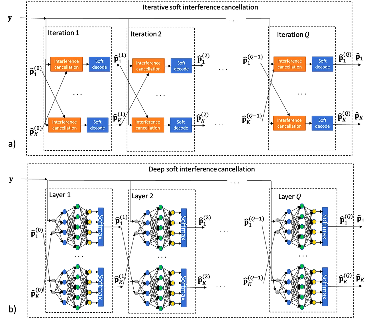
Figure 4: (a) Iterative soft interference cancellation, and (b) the DNN-based DeepSIC.

We employ modular training as described in Algorithm 2. DeepSIC uses $M=K\cdot Q$ modules, with the $(k,q)$-th module detecting the symbol of user $k$ at iteration $q$. Since only user $k^{\prime}$ is moving, we define the set of dynamic modules as $\mathcal{M}_{D}=\{(k^{\prime},q)\>|\>q\in\{1,\ldots,Q\}\}$, with all other modules being static. We define the module-wise proximal loss (7) for module $k$ at iteration $q$ as the cross entropy

$$\hat{\mathcal{L}}_{j}({\boldsymbol{\varphi}}^{k,q})=-\sum_{i=1}^{B}\log\hat{P}_{{\boldsymbol{\varphi}}^{k,q}}({\boldsymbol{y}}_{i,j},\{\hat{{\boldsymbol{p}}}_{i,j}^{\tilde{k},q-1}\}_{\tilde{k}\neq k}|\bar{{\boldsymbol{s}}}_{i,j}),$$ (8)

where $\hat{{\boldsymbol{p}}}^{\tilde{k},q-1}$ is the estimated symbol probability for the $\tilde{k}$th user at iteration $q-1$. The module-wise parameter vector ${\boldsymbol{\varphi}}_{j+1}^{k,q}$ for each $(k,q)\in\mathcal{M}_{D}$ is obtained from $I$ gradient descent iterations

$${\boldsymbol{\varphi}}_{j+1}^{k,q}={\boldsymbol{\theta}}^{k,q}_{j+1}-\kappa^{k,q}\nabla_{{\boldsymbol{\theta}}^{k,q}}\hat{\mathcal{L}}_{j}({\boldsymbol{\varphi}}^{k,q}_{j+1})$$ (9)

with ${\boldsymbol{\theta}}^{k,q}_{j+1}$ being optimized via (7), namely,

$${\boldsymbol{\theta}}_{j+1}^{k,q}=\mathop{\arg\min}\limits_{{\boldsymbol{\theta}}^{k,q}}\sum\limits_{\{({\boldsymbol{s}}_{j^{\prime}},{{\boldsymbol{y}}}_{j^{\prime}}),({\boldsymbol{s}}_{j^{\prime}+1},{{\boldsymbol{y}}}_{j^{\prime}+1})\}\in\mathcal{D}_{j}}\hat{\mathcal{L}}_{j^{\prime}+1}({\boldsymbol{\varphi}}^{k,q}={\boldsymbol{\theta}}^{k,q}-\kappa^{k,q}\nabla_{{\boldsymbol{\theta}}^{k,q}}\hat{\mathcal{L}}_{j^{\prime}}({\boldsymbol{\theta}}^{k,q})).$$ (10)

We note that problem (10) uses all previous data up to time $j+1$; while (9) only uses only data from block $j$ for the local update.

IV-C Discussion

Modular training via Algorithm 2 exploits the model-based structure of hybrid DNN receivers, applying Algorithm 2 to the subset of relevant modules in the overall network, i.e., it uses the same data as in Algorithm 1 while adapting less parameters, thus gaining in convergence speed and accuracy of the trained model. The exact portion of the overall parameters is dictated by the ratio of the mobile users to the overall users in the network. The smaller the ratio is, the more one can benefit from modular training. We validate the benefits of modular training in Subsection V-G and show that this approach can decrease the average BER significantly. Indeed, our experimental results demonstrate that the proposed approach successfully translates the prior knowledge on the nature of the variations into improved performance, particularly when dealing with short blocks, i.e. short coherence duration of rapidly varying channels.

This modular training approach can be viewed as a form of transfer learning, as it trains online only parts of the parameters. Yet, it is specifically tailored towards interpretable architectures, adapting internal sub-modules of the overall network, as opposed to the common transfer learning approach of retraining the output layers. For instance, the suggested method trains the sub-modules associated with all mobile users separately in an iterative fashion, building upon the fact that each module ${\boldsymbol{\varphi}}^{k,q}$ should produce a soft estimate of ${\boldsymbol{S}}_{k}$. Modular training can also be enhanced to carry out some final tuning of the overall network since, e.g., the channels of the mobile users is expected to also affect how their interference is canceled when recovering the remaining users via the sub-modules which are not adapted online. Finally, it is noted that this approach relies on knowledge of the mobile user, and thus incorrect knowledge of $k^{\prime}$ is expected to affect the accuracy of the trained receiver. We leave the study of the resilience of modular training and the aforementioned extensions for future work.

V Numerical Evaluations

In this section we numerically evaluate the proposed online adaptation scheme in finite-memory SISO channels and in memoryless multi-user MIMO setups. We first describe the receivers compared in our experimental study, detailing the architectures in Subsection V-A and the training methods in Subsection V-B. Then, we present the main simulation results for evaluating online meta-learning on linear synthetic channels, non-linear synthetic channels, and channels obeying the COST 2100 model in Subsections V-C to V-E. Finally, we numerically evaluate Algorithm 2 which combines online meta-learning with the modular training in Subsection V-G.

V-A Evaluated Receivers

The receiver algorithms used in our experimental study are tailored to the considered settings:

V-A1 Finite-Memory SISO Channels

We compare two DNN-based receivers for SISO settings:

• The ViterbiNet equalizer, proposed in [47], which is a DNN-based Viterbi detector for finite-memory channels of the form (1) [53]: The Viterbi equalizer (from which ViterbiNet originates) solves the maximum likelihood sequence detection problem

  $$\hat{{\boldsymbol{s}}}_{j} =\mathop{\arg\min}_{{\boldsymbol{s}}\in\mathcal{S}}\left\{-\sum\limits_{i=1}^{B}\log p_{{{\boldsymbol{Y}}_{i,j}|\bar{{{\boldsymbol{S}}}}_{i-L+1,j},\ldots,\bar{{{\boldsymbol{S}}}}_{i,j}}}\left({\boldsymbol{y}}_{i,j}|\bar{{\boldsymbol{s}}}_{i-L+1,j},\ldots,\bar{{\boldsymbol{s}}}_{i,j}\right)\right\}.$$ (11)

  ViterbiNet computes each log likelihood using a DNN that requires no knowledge of the channel distributions $p_{{{\boldsymbol{Y}}_{j}|\bar{{{\boldsymbol{S}}}}_{i-L+1,j},\ldots,\bar{{{\boldsymbol{S}}}}_{i,j}}}$. This internal DNN is implemented using three fully-connected layers of sizes $1\times 100$, $100\times 50$, and $50\times|\mathcal{S}|^{L}$, with activation functions set to sigmoid (after first layer), ReLU (after second layer), and softmax output layer.

• A recurrent neural network symbol detector, comprised of a sliding-window long short-term memory (LSTM) classifier with two hidden layers of 256 cells and window size $L$, representing a black-box DNN benchmark [73].

The Viterbi equalizer with complete knowledge of the channel is used as a baseline method.

V-A2 Memoryless MIMO Channels

We evaluate two DNN-based MIMO receivers:

• The DeepSIC receiver detailed in Subsection IV-B: The building blocks of DeepSIC are implemented using three fully-connected layers: An $(N+K-1)\times 100$ first layer, a $100\times 50$ second layer, and a $50\times|\mathcal{S}|$ third layer, with a sigmoid and a ReLU intermediate activation functions, respectively. The number of iterations is set to $Q=5$.

• A ResNet10 black-box neural network, which is based on the DeepRX architecture proposed in [43]: The architecture is comprised of 10 residual blocks [74], each block has two convolutional layers with 3x3 kernel, one pixel padding on both sides, and no bias terms, with a ReLU in-between. A 2D batch normalization follows each convolutional layer.

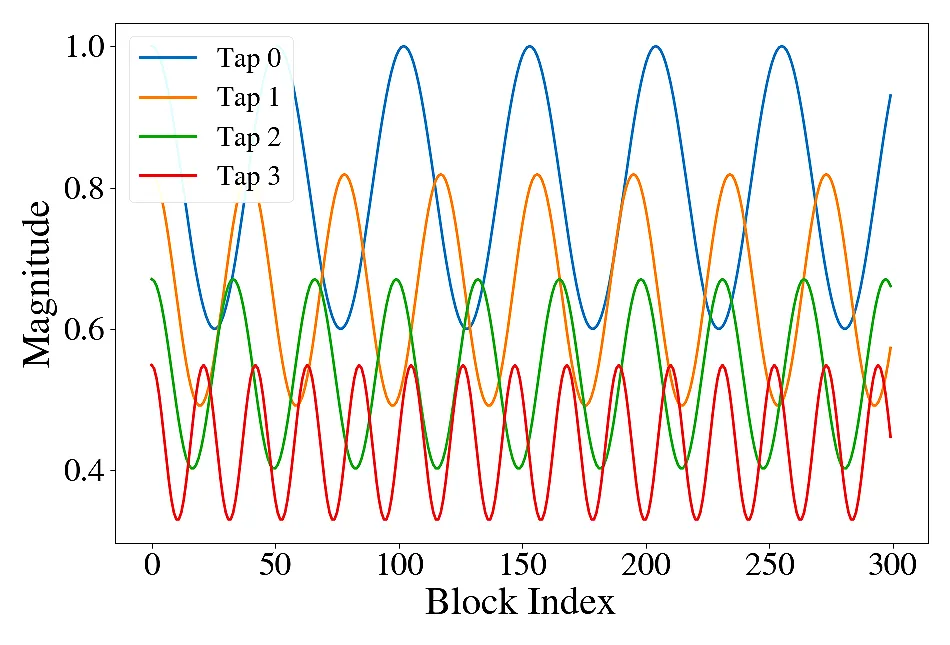
(a) Synthetic training channel.

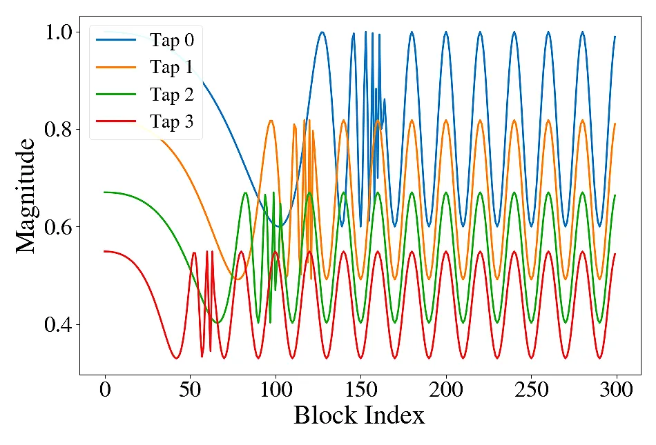
(b) Synthetic test channel.

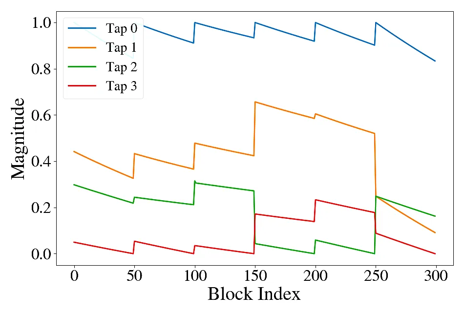
(c) COST 2100 channel.

Figure 5: Examples of time-varying channels: channel coefficients versus block index.

V-B Training Methods

Before the test phase begins, we generate a set $\mathcal{D}_{0}$ of $T_{p}$ pilot blocks. We then use the following methods for adapting the deep receivers:

• Joint training: The DNN is trained on $\mathcal{D}_{0}$ only by minimizing the empirical cross-entropy loss, and no additional training is performed in the test phase.

• Online training [47]: The DNN is initially trained on $\mathcal{D}_{0}$ by minimizing the empirical cross-entropy loss. Then, during test, the DNN parameter vector ${\boldsymbol{\varphi}}_{j}$ is re-trained on each successfully decoded data block and on each incoming pilot block as specified in (4), using ${\boldsymbol{\varphi}}_{j}$ in lieu of ${\boldsymbol{\theta}}_{j+1}$.

• Online meta-learning: Here, we first meta-train ${\boldsymbol{\theta}}_{0}$ with $\mathcal{D}_{0}$ similar to (5) as

  $${\boldsymbol{\theta}}_{0}=\mathop{\arg\min}_{{\boldsymbol{\theta}}}\sum_{\{({\boldsymbol{s}}_{j^{\prime}},{{\boldsymbol{y}}}_{j^{\prime}}),({\boldsymbol{s}}_{j^{\prime}+1},{{\boldsymbol{y}}}_{j^{\prime}+1})\}\in\mathcal{D}_{0}}\mathcal{L}_{j^{\prime}+1}({\boldsymbol{\varphi}}={\boldsymbol{\theta}}-\kappa\nabla_{{\boldsymbol{\theta}}}\mathcal{L}_{j^{\prime}}({\boldsymbol{\varphi}}={\boldsymbol{\theta}})).$$

  This process yields the initial hyperparameters ${\boldsymbol{\theta}}_{0}$. Then, during test, Algorithm 1 is used with online learning every block and online meta-learning every $F=5$ blocks. The number of online meta-learning updates equals that of online training, thus inducing a relative small overhead due to its additional computations. The combination of online meta-learning with ViterbiNet is henceforth referred to as Meta-ViterbiNet, while the DeepSIC receiver trained with this approach is coined Meta-DeepSIC.

All training methods use the Adam optimizer [75] with $I_{\rm sgd}=200$ iterations and learning rate $\eta=10^{-3}$; for meta-learning, we set the meta-learning rate to $\kappa=10^{-1}$ and the iterations to $I_{\rm meta}=200$. Both meta-learning and online learning employ a batch size of $64$ symbols. These values were set empirically such that the receivers’ parameters approximately converge at each time step (for both meta-learning and online learning). In case of the online training or meta-training schemes, re-training occurs if the normalized bits difference between the re-encoded word and the hard-decision of the channel word is smaller than the threshold of $0.02$. The complete simulation parameters can also be found in the source code available on GitHub.

V-C Linear Synthetic Channel Results

We begin by evaluating Algorithm 1 on synthetic time-varying linear channels with additive Gaussian noise, considering a finite-memory SISO setting and a memoryless MIMO setup.

V-C1 SISO Finite-Memory Channels

Recalling Fig. 1, we transmit $T_{p}=T_{d}=300$ blocks comprised of $B=136$ symbols, i.e., a relatively short coherence duration for the time-varying channel. Each block includes $120$ information bits, encoded using a Reed-Solomon [17,15] code with two parity symbols with binary phase shift keying (BPSK) modulation, i.e., $\mathcal{S}=\{\pm 1\}$.

We consider a linear Gaussian channel, whose input-output relationship is given by

$${{\boldsymbol{Y}}}_{i,j}=\sum_{l=0}^{L-1}h_{l,j}S_{i-l,j}+w_{i,j},$$ (12)

where ${\boldsymbol{h}}_{j}=[h_{0,j},\ldots,h_{L-1,j}]^{T}$ are the real channel taps, and $w_{i,j}$ is additive zero-mean white real Gaussian noise with variance $\sigma^{2}$. The channel memory is $L=4$ with the taps $\{h_{l,j}\}$ generated using a synthetic model representing oscillations of varying frequencies. Here, the signals received during the pilots used for initial training $(\mathcal{D}_{0})$ are subject to the time-varying channel whose taps are illustrated in Fig. 5(a); while we use the taps in Fig. 5(b) for testing. This channel represents oscillations of varying frequencies.

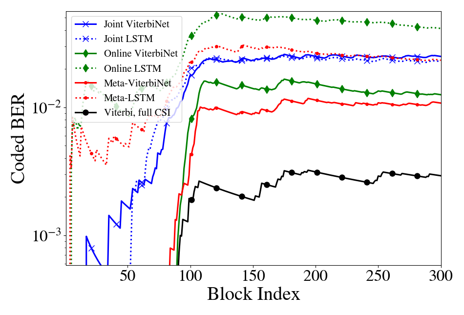
(a) Coded BER vs. block index, ${\rm SNR}=12$ dB.

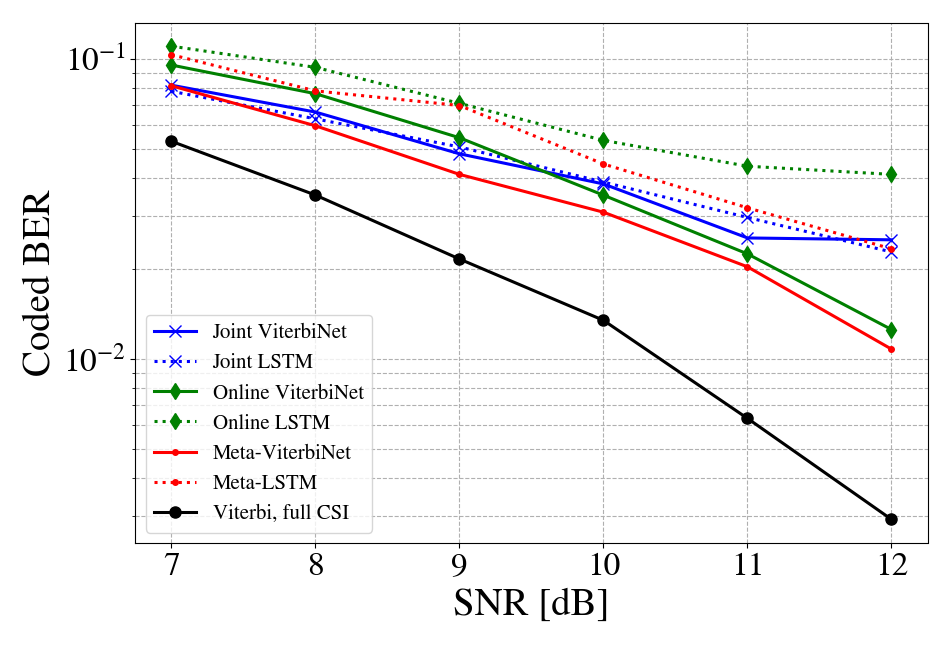
(b) Coded BER after 300 blocks vs. SNR.

Figure 6: SISO synthetic linear Gaussian channel, $B=136$.

In Fig. 6(a) we plot the evolution of the average coded BER of the considered receivers when the signal-to-noise ratio (SNR), defined as $1/\sigma^{2}$, is set to $12$ dB. Fig. 6(a) shows that Meta-ViterbiNet significantly outperforms its benchmarks, demonstrating the gains of the proposed online meta-learning training and its suitability when combined with receiver architectures utilizing relatively compact DNNs. In particular, it is demonstrated that each of the ingredients combined in Meta-VitebiNet, i.e., its model-based architecture, the usage of self-supervision, and the incorporation of online meta-learning, facilitates operation in time-varying conditions: The ViterbiNet architecture consistently outperforms the black-box LSTM classifier; Online training yields reduced BER as compared to joint learning; and its combination with meta-learning via Algorithm 1 yields the lowest BER values. To further validate that these gains also hold for different SNRs, we show in Fig. 6(b) the average coded BER of the evaluated receivers after 300 blocks, averaged over 5 trials. We observe in Fig. 6(b) that for SNR values larger than $8$ dB, Meta-ViterbiNet consistently achieves the lowest BER values among all considered data-driven receivers, with gains of up to 0.5dB over the online training counterpart.

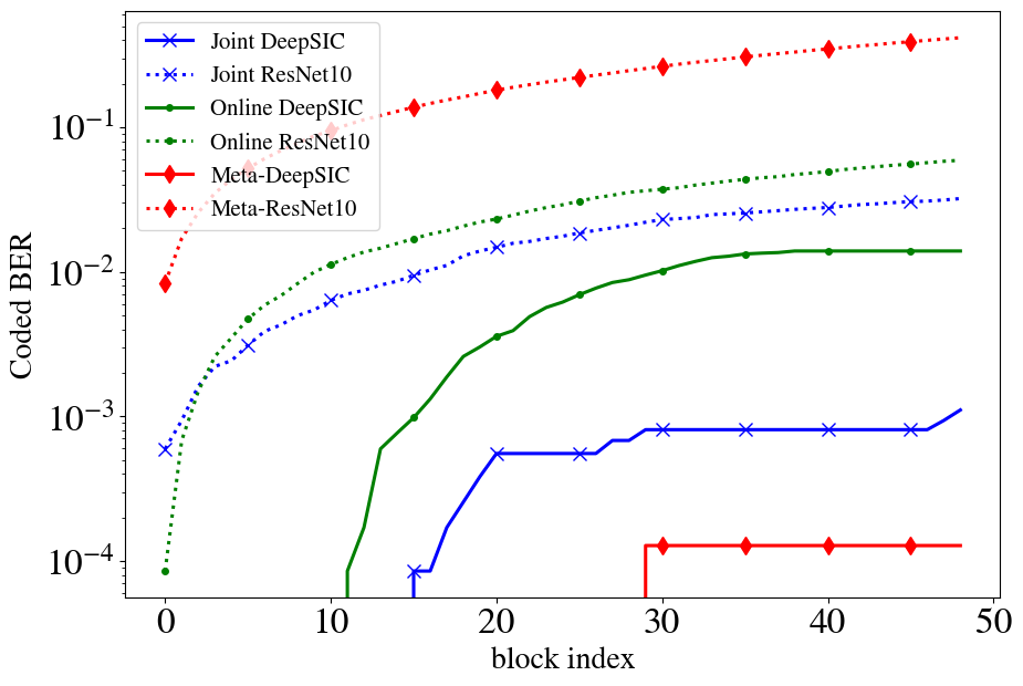
(a) Coded BER vs. block index, ${\rm SNR}=14$ dB.

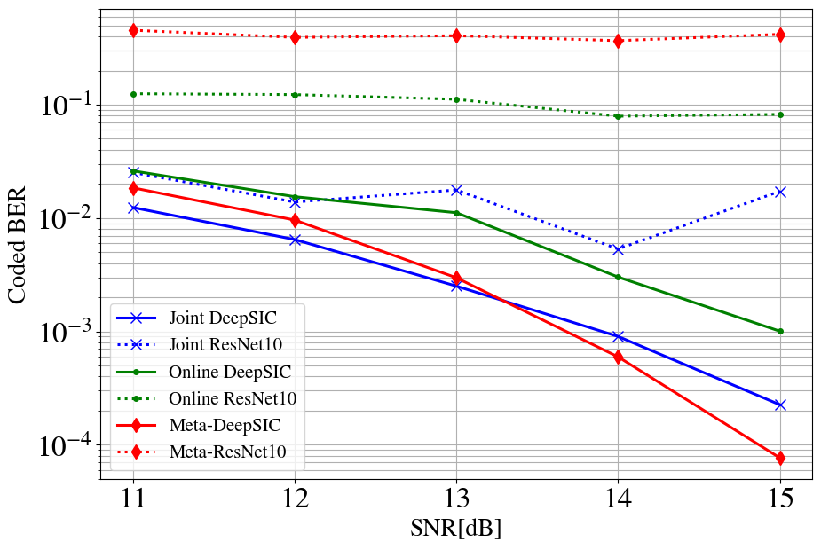
(b) Coded BER after 50 blocks vs. SNR.

Figure 7: MIMO synthetic linear Gaussian channel, $B=152$.

V-C2 Memoryless MIMO Channels

For the MIMO setting, use $T_{p}=T_{d}=50$ blocks. The block length is set to $B=152$ symbols, encoding 120 information bits with Reed-Solomon [19,15] code. The input-output relationship of a the memoryless Gaussian MIMO channel is given by

$${{\boldsymbol{Y}}}={\boldsymbol{H}}{{\boldsymbol{S}}}+{\boldsymbol{W}},$$ (13)

where ${\boldsymbol{H}}$ is a known deterministic $N\times K$ channel matrix, and ${\boldsymbol{W}}$ consists of $N$ i.i.d Gaussian RVs. We set the number of users and antennas to $N=K=4$. The channel matrix ${\boldsymbol{H}}$ models spatial exponential decay, and its entries are given by $\left({\boldsymbol{H}}\right)_{n,k}=e^{-|n-k|}$, for each $n\in\{1,\ldots,N\}$, $k\in\{1,\ldots,K\}$. The transmitted symbols are generated from a BPSK constellation in a uniform i.i.d. manner, i.e., $\mathcal{S}=\{\pm 1\}$.

The numerical results for the memoryless Gaussian channel (13) are depicted in Fig. 7. Note that Fig. 7(a) shows the average coded BER of the receivers for ${\rm SNR}=14$ dB for a single trial, while Fig. 7(b) shows a sweep over a range of SNR values after 50 blocks, averaged over 10 trials. Similarly to Meta-ViterbiNet in the finite-memory SISO setting, Meta-DeepSIC outperforms all other training methods in medium to high SNRs. Here, the black-box architectures perform quite poorly, unable to compete with the model-based deep architecture of DeepSIC due to short blocklengths and the highly limited volumes of data used for training. Training DeepSIC with Algorithm 1 outperforms the joint training approach with gains of up to 1dB, and with gains of 1.5dB over online training, which notably struggles in tracking such rapidly time-varying and challenging conditions.

V-D Non-Linear Synthetic Channel Results

Next, we evaluate the proposed online meta-learning scheme in non-linear synthetic channels, where one can greatly benefit from the model-agnostic nature of DNN-based receivers.

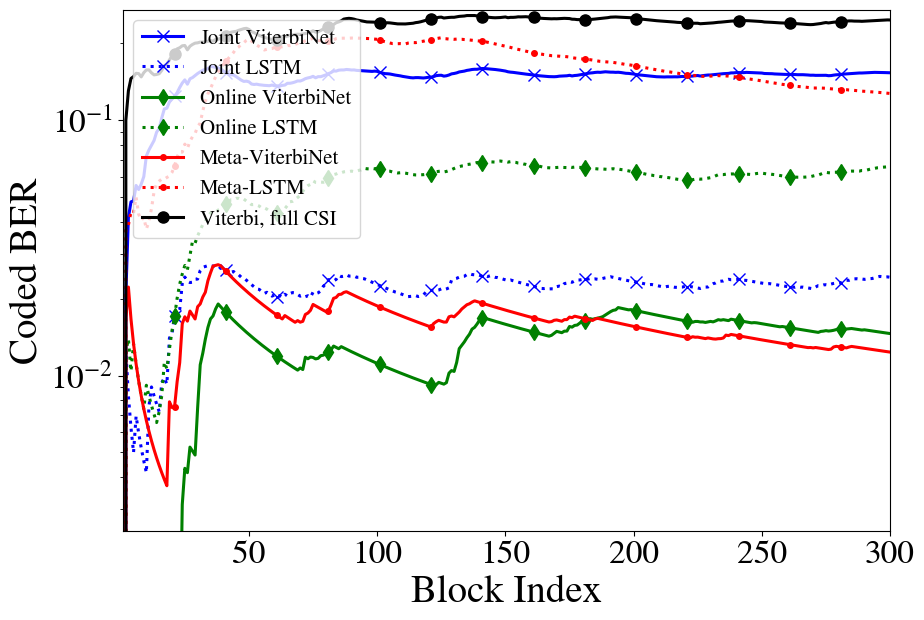
(a) Coded BER vs. block index, ${\rm SNR}=12$ dB.

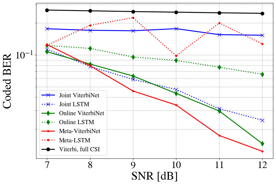
(b) Coded BER after 300 blocks vs. SNR.

Figure 8: SISO synthetic non-linear Gaussian channel, $B=136$.

V-D1 SISO Finite-Memory Channels

To check the robustness of our method in a non-linear case, we generate a non-linear channel by applying a non-linear transformation to synthetic channel in (12). The resulting finite-memory SISO channel is give by

$${{\boldsymbol{Y}}}_{i,j}=\tanh{\Big{(}C\cdot\Big{(}\sum_{l=0}^{L-1}h_{l,j}S_{i-l,j}+w_{i,j}\Big{)}\Big{)}}.$$ (14)

This operation may represent, e.g., non-linearities induced by the receiver acquisition hardware. The hyperparameter $C$ stands for a power attenuation at the receiver, and chosen empirically as $C=\frac{1}{2}$. All other hyperparameters and settings are the same as those used in the previous subsection. This simulation shows a consistent gain of around $0.75$dB over the SNRs with values of $8$dB - $12$dB, as observed in Fig. 8.

V-D2 Memoryless MIMO Channels

Similarly to the SISO case, we simulate a non-linear MIMO channel from (13) via

$${{\boldsymbol{Y}}}=\tanh{\Big{(}C\cdot\Big{(}{\boldsymbol{H}}{{\boldsymbol{S}}}+{\boldsymbol{W}}\Big{)}\Big{)}},$$ (15)

with $C=\frac{1}{2}$ and the remaining simulation settings are chosen as in Subsection V-C. The numerical results for this channel are illustrated in Fig. 9, showing that the superiority of our approach is maintained in non-linear setups. The right part shows an average over 20 trials, while the left graph corresponds to an exemplary trial. In particular, we note that gains of up to 0.5dB in high SNRs are achieved compared with online training, while the gap from joint method is around 0.25dB. Here, our gain becomes apparent as the SNR increases.

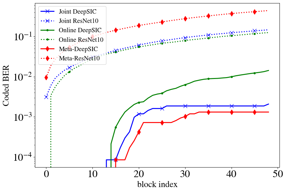
(a) Coded BER vs. block index, ${\rm SNR}=14$ dB.

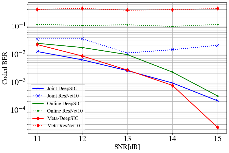
(b) Coded BER after 50 blocks vs. SNR.

Figure 9: MIMO synthetic non-linear Gaussian channel, $B=152$.

V-E COST 2100 Channel Results

Next, we consider channels generated using the COST 2100 geometry-based stochastic channel model [70], which is widely used in indoor wireless communications.

V-E1 SISO Finite-Memory Channels

We generate each realization of the taps using an indoor hall $5$ GHz setting with single-antenna elements. We use the same block length and number of error-correction symbols, as well as the same initial training set $\mathcal{D}_{0}$ as in the synthetic model. This setting may represent a user moving in an indoor setup while switching between different microcells. Succeeding in this scenario requires high adaptivity since there is considerable mismatch between the train and test channels. The test is carried out using a sequence of difference realizations illustrated in Fig. 5(c), whereas the initial training still follows the taps illustrated in Fig. 5(a). The two main figures, Fig. 10(a) and Fig. 10(b) illustrate gains of up to 0.6dB by using our scheme compared to other methods.

(a) Coded BER vs. block index, ${\rm SNR}=12$ dB.

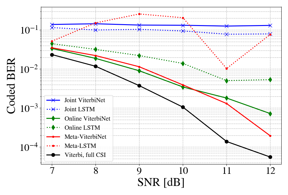
(b) Coded BER after 300 blocks vs. SNR.

Figure 10: SISO COST 2100 channel, $B=136$.

V-E2 Memoryless MIMO Channels

For the current MIMO setting, we compose the test channels from only $T_{p}=T_{d}=40$ blocks and increase the number of users and antennas to $N=K=8$. To simulate the channel matrix ${\boldsymbol{H}}$, we follow the above SISO description and create $8\times 8=64$ SISO COST 2100 channels; Each simulated channel corresponds to a single entry $\left({\boldsymbol{H}}\right)_{n,k}$ with $n\in\{1,\ldots,N\}$, $k\in\{1,\ldots,K\}$. Moving to results, one may observe the respective graphs Fig. 11(a) and Fig. 11(b), which show an unusual gain of up to 2dB approximately, as the joint and online methods are unable to compete with the proposed meta approach. The results here are averaged over 20 trials.

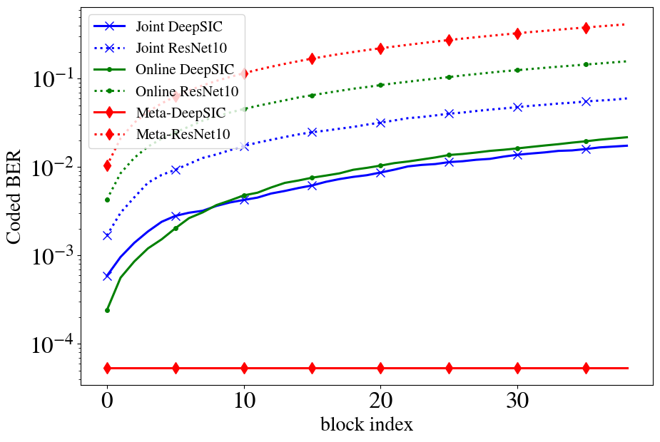
(a) Coded BER vs. block index, ${\rm SNR}=14$ dB.

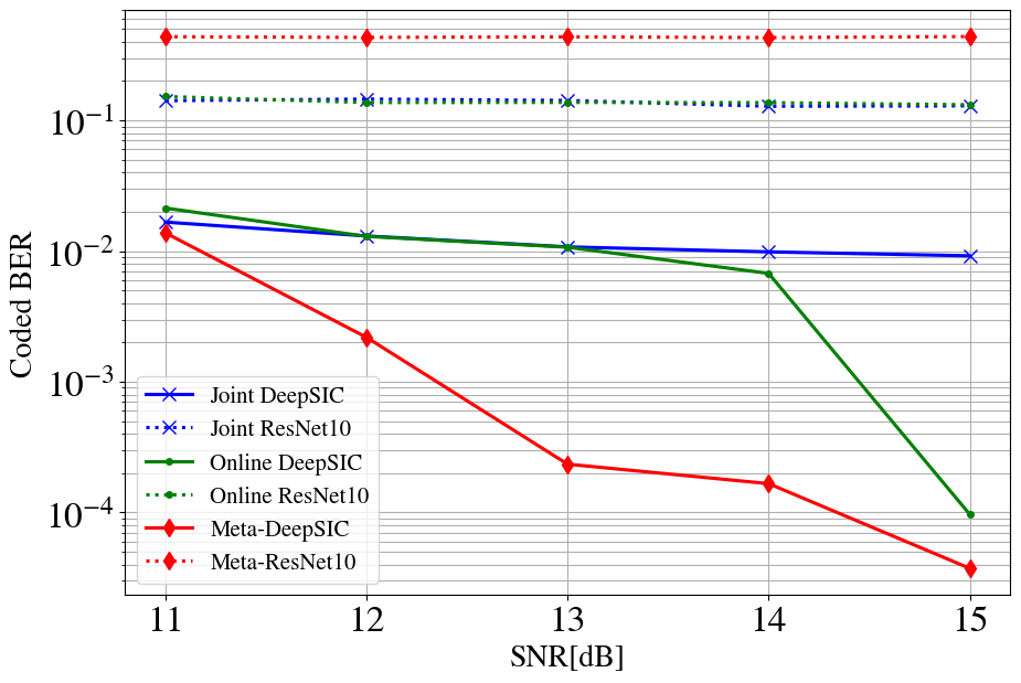
(b) Coded BER after 40 blocks vs. SNR.

Figure 11: MIMO COST 2100 channel, $B=152$.

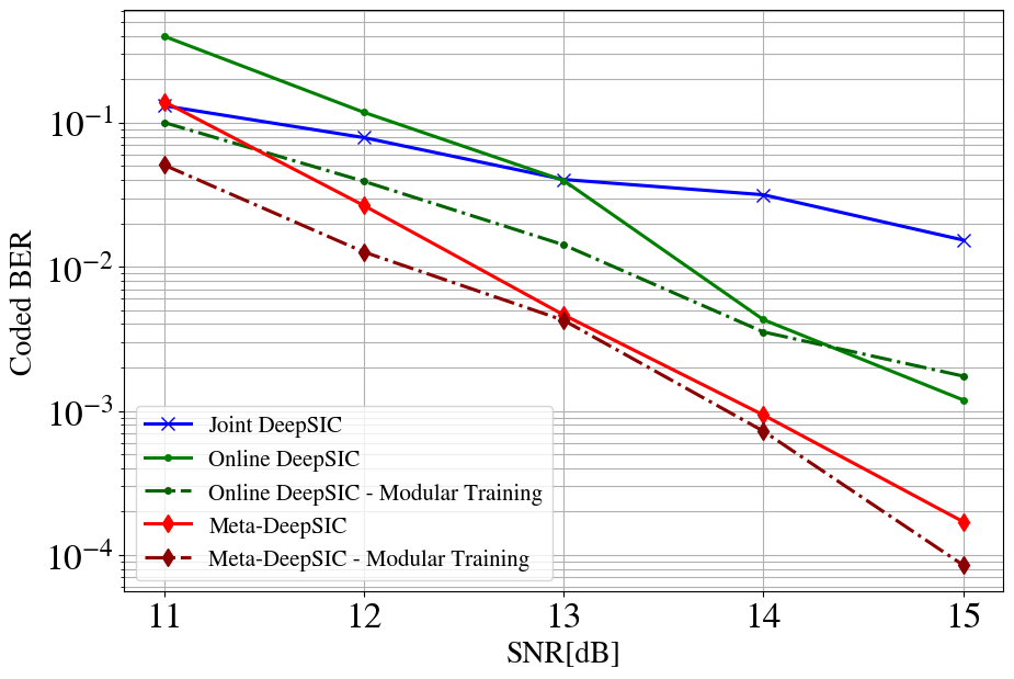
(a) Synthetic linear channel.

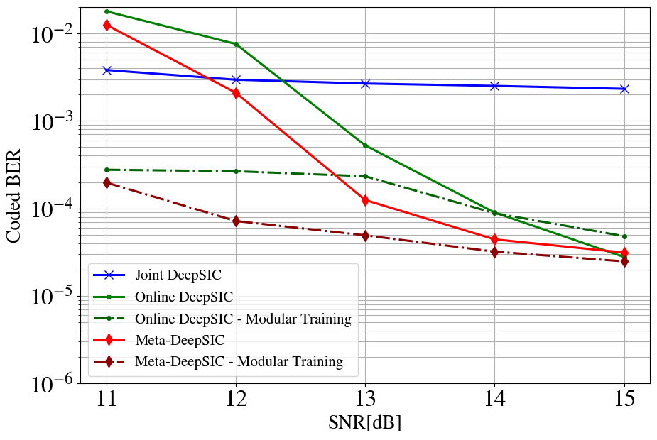
(b) COST 2100 channel.

Figure 12: Modular Training - Coded BER vs. SNR, $B=152$.

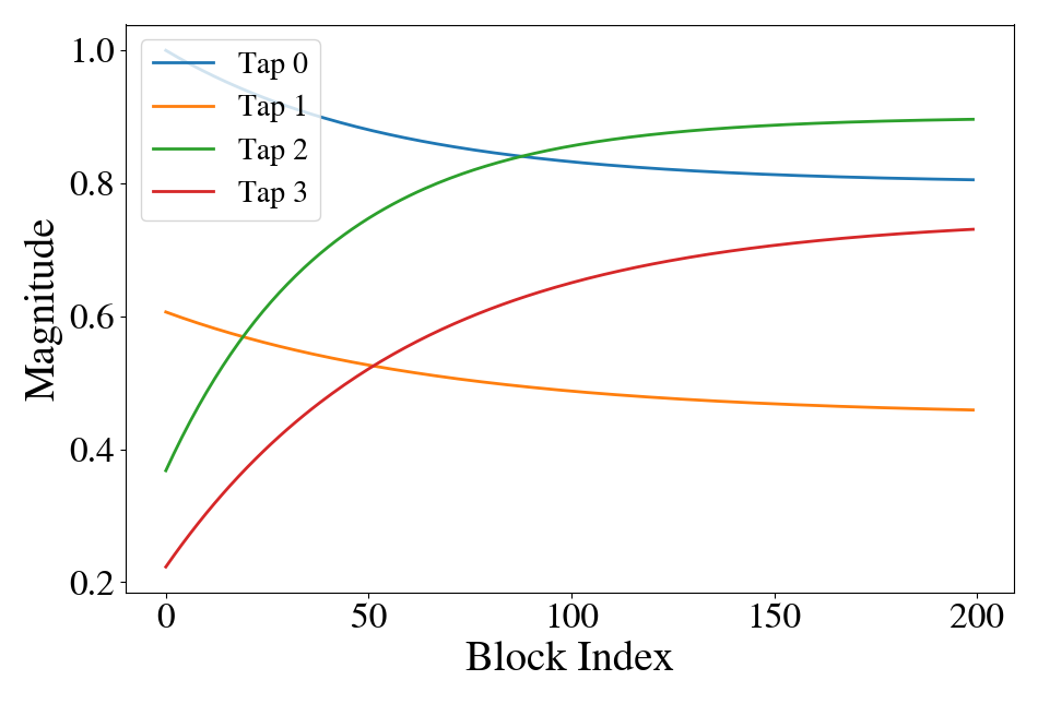
(a) SISO synthetic non-periodic channel taps.

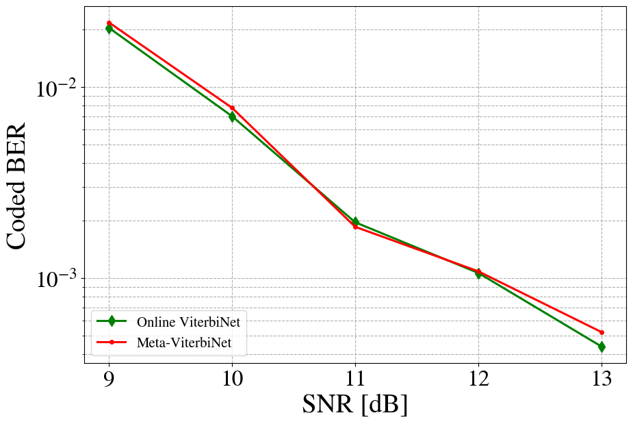
(b) Coded BER after 300 blocks vs. SNR.

Figure 13: Exploring Non-Periodic Channel Profile, $B=136$.

V-F Channel with non-Repetitive Temporal Variations

The temporal variation profiles considered so far, illustrated in Fig. 5, all exhibit periodic temporal variations, or more general patterns of variation of the channel. To elaborate on the importance of such patterns in enabling the benefits of meta-learning, we now simulate a SISO linear Gaussian channel, as in Subsection V-C under the channel taps variations profile depicted in Fig. 13(a). The channel variations are unstructured, limiting the ability of meta-learning to predict the variation profiles from past channel realizations. In Fig. 13(b), we compare the ViterbiNet architecture trained online in a self-supervised manner both with and without predictive meta-learning. The figure demonstrates that predictive meta-learning is indeed beneficial when the temporal variations exhibit useful structure across blocks, enabling meta-generalization [76].

V-G Modular Training Results

To evaluate the modular training methods proposed in Section IV, we next consider a multi-user MIMO setting. Here, the temporal variations stem from the fact that only a single user is changing ($k^{\prime}=2$), with the other ones being static. The receiver uses DeepSIC, and knows the identity of the dynamic user. We numerically compare the gains of exploiting this knowledge using Algorithm 2, as well as the individual gains of combining modular training with predictive meta-learning compared with online adapting solely the network weights.

Fig. 12 shows the two compared methods – online-training and (predictive) online-meta training – executed either with or without modular training (Algorithm 2) for the synthetic linear channel (Fig. 12(a)) and the COST 2100 channel (Fig. 12(b)). We also plot the joint training method for completeness. One may observe that our modular meta-training achieves superior results compared to the other methods. As depicted in Fig. 12(a), one may gain additional 0.3 dB under the meta-learning scheme by employing the modular training approach, for low and high SNR values. In medium SNR, one is expected to achieve similar results to the non-modular method. On the other hand, Fig. 12(b) shows that the combined approach can provide substantial benefits, due to the rapid variations of the channel. Specifically, the modular gains appear in low to medium SNR, while the gains of the meta-learning stage appear for the higher SNR values. The gain in both scenarios for the two-stage approach versus simple online training is up to 2.5 dB. These results indicate the gains of our two-stage approach, and show that Algorithm 2 translates the interpretable modular architecture of DeepSIC into improved online adaptation in the presence of temporal variations due to a combination of mobile and static users.

V-H Complexity Analysis

We now compare the complexity of the different training methods in terms of the number of iterations. Joint training does not apply re-training, and hence it has the lowest possible complexity at test time. For self-supervised online training, re-training is done for $I_{\rm sgd}$ SGD iterations at every coherence interval. The proposed predictive meta-learning scheme performs online training at each coherence interval with $I_{\rm sgd}$ iterations. Furthermore, it optimizes the initial weights via $I_{\rm meta}$ learning iterations, which are repeated periodically every $F$ blocks. Consequently, meta-learning applies on average $\frac{I_{\rm sgd}+I_{\rm meta}}{F}$ iterations on each coherence duration.

Nonetheless, the proposed meta-learning update, applied once each $F$ block, can help online training, applied on each block, to converge more quickly. As a result, while the proposed approach comes at the cost of $I_{\rm meta}/F$ additional gradient computations per block on average, it can operate with fewer online training iterations, $I_{\rm sgd}$. Therefore, meta-learning can in fact reduce the overall number of gradient steps as compared with online training.

V-I Meta-Learning Frequency Effect

We conclude our numerical evaluations by studying the effect of changing the meta-learning frequency $F$. To this end, fixing ${\rm SNR}=10$ dB, $B=136$, as in Subsection V-C and Subsection V-D, Fig. 14 illustrates the coded BER after 1000 blocks, plotted against values of $F\in\{5,10,15,25,50\}$. We observe that a lower value of $F$ yields a lower BER for both the linear and non-linear cases. It is also observed that increasing the value of $F$ causes the performance of meta-learning to be within a minor gap as that of the online training. The small difference follows since, while for large values of $F$, meta-learning is rarely carried out, the initial weights utilized at each block differ from that of conventional online training. In particular, when meta-learning is employed, the same initial weights are used for consecutive $F$ blocks, while online training sets the initial weights at block $j$ to be those utilized in block $j-1$.

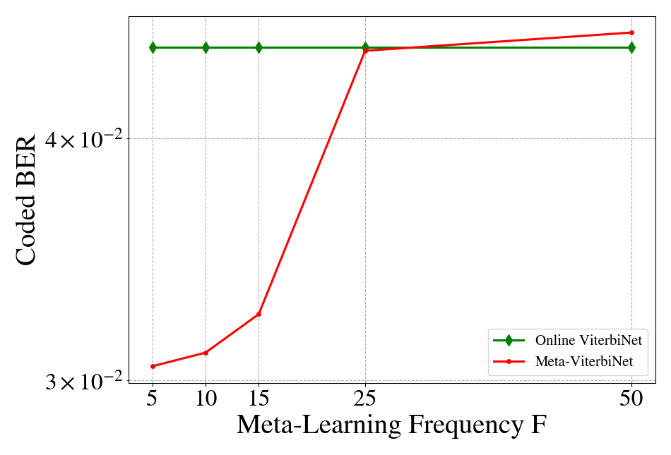
(a) SISO synthetic linear Gaussian channel.

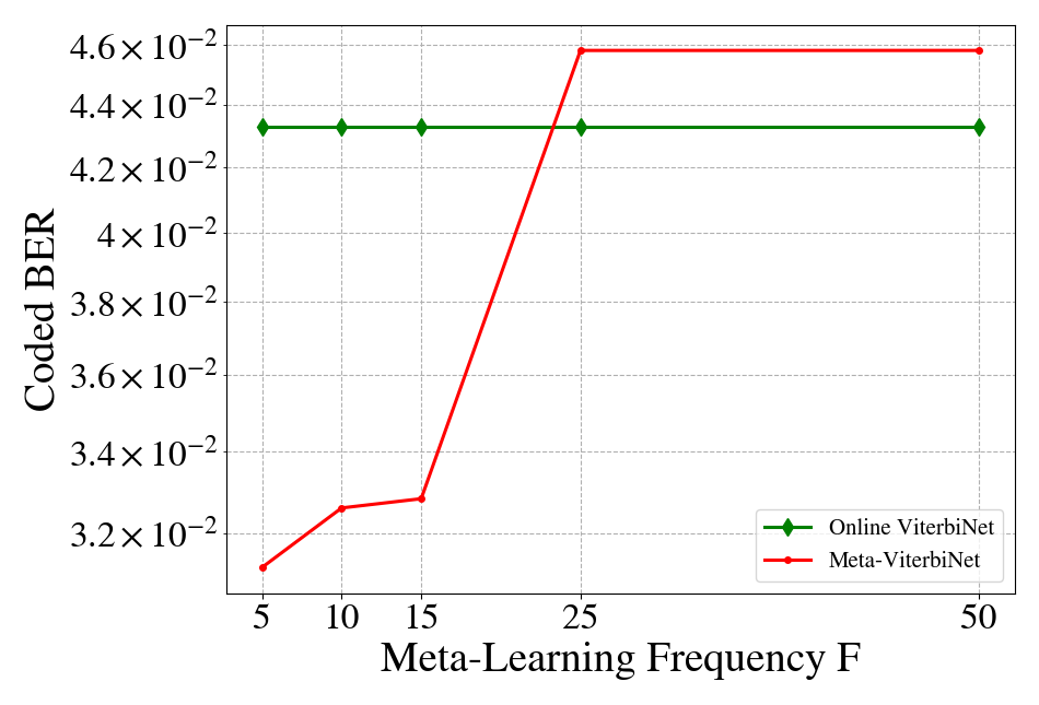
(b) SISO synthetic non-linear Gaussian channel.

Figure 14: Coded BER versus meta-learning frequency $F$; ${\rm SNR}=10$ dB, $B=136$.

VI Conclusion

In this paper, we proposed a two-stage training method whose goal is to aid DNN-based receivers in tracking time-varying channels. The first part of the paper introduces a predictive meta-learning method that incorporates both short-term and long-term relations between the symbols and the received channel values. This method yields initial weights such that training on a block transmitted over some channel minimizes the error on the block transmitted over the next channel. The approach is generic and applicable to any DNN-based receiver. Then, we have introduced a modular training scheme that exploits the interpretable structure of model-based deep receivers, and applies meta-learning to allow efficient adaptation only for the subset of modules that suffers mostly from rapidly varying channels. Numerical studies demonstrate that, by properly integrating these methods, model-based deep receivers trained with the meta-training algorithm and modular training outperform existing self-supervision and joint learning approaches [23, 39, 47, 48].

References

- [1] T. Raviv, S. Park, N. Shlezinger, O. Simeone, Y. C. Eldar, and J. Kang, “Meta-ViterbiNet: Online meta-learned Viterbi equalization for non-stationary channels,” in Proc. IEEE ICC, 2021.
- [2] J. Xia, K. He, W. Xu, S. Zhang, L. Fan, and G. K. Karagiannidis, “A MIMO detector with deep learning in the presence of correlated interference,” IEEE Trans. Veh. Technol., vol. 69, no. 4, pp. 4492–4497, 2020.
- [3] N. Shlezinger, G. C. Alexandropoulos, M. F. Imani, Y. C. Eldar, and D. R. Smith, “Dynamic metasurface antennas for 6G extreme massive MIMO communications,” IEEE Wireless Commun., vol. 28, no. 2, pp. 106–113, 2021.
- [4] G. C. Alexandropoulos, N. Shlezinger, I. Alamzadeh, M. F. Imani, H. Zhang, and Y. C. Eldar, “Hybrid reconfigurable intelligent metasurfaces: Enabling simultaneous tunable reflections and sensing for 6G wireless communications,” arXiv preprint arXiv:2104.04690, 2021.
- [5] N. Farsad and A. Goldsmith, “Neural network detection of data sequences in communication systems,” IEEE Trans. Signal Process., vol. 66, no. 21, pp. 5663–5678, 2018.
- [6] N. Shlezinger, Y. C. Eldar, and M. R. Rodrigues, “Asymptotic task-based quantization with application to massive MIMO,” IEEE Trans. Signal Process., vol. 67, no. 15, pp. 3995–4012, 2019.
- [7] N. Shlezinger, Y. C. Eldar, and S. P. Boyd, “Model-based deep learning: On the intersection of deep learning and optimization,” IEEE Access, vol. 10, 2022.
- [8] N. Shlezinger, J. Whang, Y. C. Eldar, and A. G. Dimakis, “Model-based deep learning,” arXiv:2012.08405, 2020.
- [9] Y. C. Eldar, A. Goldsmith, D. Gündüz, and H. V. Poor, Machine Learning and Wireless Communications. Cambridge University Press, 2022.
- [10] S. Cammerer, F. A. Aoudia, S. Dörner, M. Stark, J. Hoydis, and S. Ten Brink, “Trainable communication systems: Concepts and prototype,” IEEE Trans. Commun., vol. 68, no. 9, pp. 5489–5503, 2020.
- [11] H. Ye, G. Y. Li, B.-H. F. Juang, and K. Sivanesan, “Channel agnostic end-to-end learning based communication systems with conditional gan,” in Proc. IEEE Globecom, 2018.
- [12] H. Ye, G. Y. Li, and B.-H. Juang, “Deep learning based end-to-end wireless communication systems without pilots,” IEEE Trans. on Cogn. Commun. Netw., vol. 7, no. 3, pp. 702–714, 2021.
- [13] N. Farsad, M. Rao, and A. Goldsmith, “Deep learning for joint source-channel coding of text,” in Proc. IEEE ICASSP, 2018, pp. 2326–2330.
- [14] E. Nachmani, E. Marciano, L. Lugosch, W. J. Gross, D. Burshtein, and Y. Be’ery, “Deep learning methods for improved decoding of linear codes,” IEEE J. Sel. Topics Signal Process., vol. 12, no. 1, pp. 119–131, 2018.
- [15] T. Gruber, S. Cammerer, J. Hoydis, and S. ten Brink, “On deep learning-based channel decoding,” in Proc. IEEE CISS, 2017.
- [16] I. Be’ery, N. Raviv, T. Raviv, and Y. Be’ery, “Active deep decoding of linear codes,” IEEE Trans. Commun., vol. 68, no. 2, pp. 728–736, 2019.
- [17] E. Nachmani and L. Wolf, “Hyper-graph-network decoders for block codes,” Advances in Neural Information Processing Systems, vol. 32, 2019.
- [18] H. He, C.-K. Wen, S. Jin, and G. Y. Li, “Deep learning-based channel estimation for beamspace mmWave massive MIMO systems,” vol. 7, no. 5, pp. 852–855, 2018.
- [19] C.-K. Wen, W.-T. Shih, and S. Jin, “Deep learning for massive MIMO CSI feedback,” vol. 7, no. 5, pp. 748–751, 2018.
- [20] D. Gündüz, P. de Kerret, N. D. Sidiropoulos, D. Gesbert, C. R. Murthy, and M. van der Schaar, “Machine learning in the air,” IEEE J. Sel. Areas Commun., vol. 37, no. 10, pp. 2184–2199, 2019.
- [21] O. Simeone, “A very brief introduction to machine learning with applications to communication systems,” IEEE Trans. on Cogn. Commun. Netw., vol. 4, no. 4, pp. 648–664, 2018.
- [22] A. Balatsoukas-Stimming and C. Studer, “Deep unfolding for communications systems: A survey and some new directions,” arXiv preprint arXiv:1906.05774, 2019.
- [23] T. O’Shea and J. Hoydis, “An introduction to deep learning for the physical layer,” IEEE Trans. on Cogn. Commun. Netw., vol. 3, no. 4, pp. 563–575, 2017.
- [24] S. Zheng, S. Wu, H. Li, C. Jiang, and X. Jing, “Deep learning-aided receiver against nonlinear distortion of hpa in ofdm systems,” in Proc. IEEE WCSP, 2021.
- [25] B. Karanov, M. Chagnon, F. Thouin, T. A. Eriksson, H. Bülow, D. Lavery, P. Bayvel, and L. Schmalen, “End-to-end deep learning of optical fiber communications,” Journal of Lightwave Technology, vol. 36, no. 20, pp. 4843–4855, 2018.
- [26] Z.-R. Zhu, J. Zhang, R.-H. Chen, and H.-Y. Yu, “Autoencoder-based transceiver design for owc systems in log-normal fading channel,” IEEE Photonics Journal, vol. 11, no. 5, pp. 1–12, 2019.
- [27] T. Uhlemann, S. Cammerer, A. Span, S. Dörner, and S. ten Brink, “Deep-learning autoencoder for coherent and nonlinear optical communication,” in ITG-Symposium, 2020.
- [28] H. Lu, W. Chen, and M. Jiang, “Deep learning aided misalignment-robust blind receiver for underwater optical communication,” IEEE Wireless Commun. Lett., vol. 10, no. 9, pp. 1984–1988, 2021.
- [29] Y. Zhang, C. Li, H. Wang, J. Wang, F. Yang, and F. Meriaudeau, “Deep learning aided OFDM receiver for underwater acoustic communications,” Applied Acoustics, vol. 187, p. 108515, 2022.
- [30] S. Khan, K. S. Khan, N. Haider, and S. Y. Shin, “Deep-learning-aided detection for reconfigurable intelligent surfaces,” arXiv preprint arXiv:1910.09136, 2019.
- [31] W. Xu, “Artificial intelligence aided receiver design for wireless communication systems,” Ph.D. dissertation, 2021.
- [32] N. Shlezinger, N. Farsad, Y. C. Eldar, and A. Goldsmith, “Learned factor graphs for inference from stationary time sequences,” IEEE Trans. Signal Process., vol. 70, pp. 366–380, 2021.
- [33] N. Farsad, N. Shlezinger, A. J. Goldsmith, and Y. C. Eldar, “Data-driven symbol detection via model-based machine learning,” arXiv preprint arXiv:2002.07806, 2020.
- [34] J. Kim, Y. Ahn, and B. Shim, “Massive data generation for deep learning-aided wireless systems using meta learning and generative adversarial network,” IEEE Trans. Veh. Technol., 2022.
- [35] T. Raviv and N. Shlezinger, “Adaptive data augmentation for deep receivers,” in Proc. IEEE SPAWC, 2022.
- [36] N. Soltani, K. Sankhe, J. Dy, S. Ioannidis, and K. Chowdhury, “More is better: Data augmentation for channel-resilient RF fingerprinting,” IEEE Commun. Mag., vol. 58, no. 10, pp. 66–72, 2020.
- [37] M. Zecchin, S. Park, O. Simeone, M. Kountouris, and D. Gesbert, “Robust bayesian learning for reliable wireless ai: Framework and applications,” arXiv preprint arXiv:2207.00300, 2022.
- [38] I. Nikoloska and O. Simeone, “Bayesian active meta-learning for black-box optimization,” in Proc. IEEE SPAWC, 2022.
- [39] J. Xia, D. Deng, and D. Fan, “A note on implementation methodologies of deep learning-based signal detection for conventional MIMO transmitters,” IEEE Trans. Broadcast., vol. 66, no. 3, pp. 744–745, 2020.
- [40] T. Raviv, N. Raviv, and Y. Be’ery, “Data-driven ensembles for deep and hard-decision hybrid decoding,” in Proc. IEEE ISIT, 2020, pp. 321–326.
- [41] S. Park, H. Jang, O. Simeone, and J. Kang, “Learning to demodulate from few pilots via offline and online meta-learning,” IEEE Trans. Signal Process., vol. 69, pp. 226 – 239, 2020.
- [42] H. He, C.-K. Wen, S. Jin, and G. Y. Li, “Model-driven deep learning for MIMO detection,” IEEE Trans. Signal Process., vol. 68, pp. 1702–1715, 2020.
- [43] M. Honkala, D. Korpi, and J. M. Huttunen, “DeepRx: Fully convolutional deep learning receiver,” IEEE Trans. Wireless Commun., vol. 20, no. 6, pp. 3925–3940, 2021.
- [44] M. Khani, M. Alizadeh, J. Hoydis, and P. Fleming, “Adaptive neural signal detection for massive MIMO,” IEEE Trans. Wireless Commun., vol. 19, no. 8, pp. 5635–5648, 2020.
- [45] N. Samuel, T. Diskin, and A. Wiesel, “Learning to detect,” IEEE Trans. Signal Process., vol. 67, pp. 2554–2564, 2019.
- [46] M. Goutay, F. A. Aoudia, J. Hoydis, and J.-M. Gorce, “Machine learning for MU-MIMO receive processing in OFDM systems,” IEEE J. Sel. Areas Commun., vol. 39, no. 8, pp. 2318–2332, 2021.
- [47] N. Shlezinger, N. Farsad, Y. C. Eldar, and A. J. Goldsmith, “ViterbiNet: A deep learning based Viterbi algorithm for symbol detection,” IEEE Trans. Wireless Commun., vol. 19, no. 5, pp. 3319–3331, 2020.
- [48] C.-F. Teng and Y.-L. Chen, “Syndrome enabled unsupervised learning for neural network based polar decoder and jointly optimized blind equalizer,” IEEE Trans. Emerg. Sel. Topics Circuits Syst., 2020.
- [49] S. Schibisch, S. Cammerer, S. Dörner, J. Hoydis, and S. ten Brink, “Online label recovery for deep learning-based communication through error correcting codes,” in Proc. IEEE ISWCS, 2018.
- [50] H. H. Mao, “A survey on self-supervised pre-training for sequential transfer learning in neural networks,” arXiv preprint arXiv:2007.00800, 2020.
- [51] A. Jaiswal, A. R. Babu, M. Z. Zadeh, D. Banerjee, and F. Makedon, “A survey on contrastive self-supervised learning,” Technologies, vol. 9, no. 1, p. 2, 2020.
- [52] H. Wang, E. Ahn, and J. Kim, “Self-supervised representation learning framework for remote physiological measurement using spatiotemporal augmentation loss,” in AAAI Conference on Artificial Intelligence, 2022.
- [53] A. Viterbi, “Error bounds for convolutional codes and an asymptotically optimum decoding algorithm,” IEEE Trans. Inf. Theory, vol. 13, no. 2, pp. 260–269, 1967.
- [54] L. Bahl, J. Cocke, F. Jelinek, and J. Raviv, “Optimal decoding of linear codes for minimizing symbol error rate,” IEEE Trans. Inf. Theory, vol. 20, no. 2, pp. 284–287, 1974.
- [55] W.-J. Choi, K.-W. Cheong, and J. M. Cioffi, “Iterative soft interference cancellation for multiple antenna systems,” in Proc. IEEE WCNC, 2000.
- [56] N. Shlezinger, N. Farsad, Y. C. Eldar, and A. J. Goldsmith, “Data-driven factor graphs for deep symbol detection,” in Proc. IEEE ISIT, 2020, pp. 2682–2687.
- [57] N. Shlezinger, R. Fu, and Y. C. Eldar, “DeepSIC: Deep soft interference cancellation for multiuser MIMO detection,” IEEE Trans. Wireless Commun., vol. 20, no. 2, pp. 1349–1362, 2021.
- [58] S. Park, O. Simeone, and J. Kang, “Meta-learning to communicate: Fast end-to-end training for fading channels,” in Proc. IEEE ICASSP, 2020.
- [59] O. Simeone, S. Park, and J. Kang, “From learning to meta-learning: Reduced training overhead and complexity for communication systems,” in IEEE 6G Wireless Summit, 2020.
- [60] Y. Jiang, H. Kim, H. Asnani, and S. Kannan, “MIND: Model independent neural decoder,” in Proc. IEEE SPAWC, 2019.
- [61] S. Park, O. Simeone, and J. Kang, “End-to-end fast training of communication links without a channel model via online meta-learning,” in Proc. IEEE SPAWC, 2020.
- [62] A. E. Kalør, O. Simeone, and P. Popovski, “Prediction of mmwave/thz link blockages through meta-learning and recurrent neural networks,” IEEE Wireless Commun. Lett., vol. 10, no. 12, pp. 2815–2819, 2021.
- [63] Y. Yuan, G. Zheng, K.-K. Wong, B. Ottersten, and Z.-Q. Luo, “Transfer learning and meta learning-based fast downlink beamforming adaptation,” IEEE Trans. Wireless Commun., vol. 20, no. 3, pp. 1742–1755, 2020.
- [64] I. Nikoloska and O. Simeone, “Fast power control adaptation via meta-learning for random edge graph neural networks,” in Proc. IEEE SPAWC, 2021, pp. 146–150.
- [65] C. Finn, P. Abbeel, and S. Levine, “Model-agnostic meta-learning for fast adaptation of deep networks,” in Proceedings of the International Conference on Machine Learning-Volume 70, 2017, pp. 1126–1135.
- [66] V. Monga, Y. Li, and Y. C. Eldar, “Algorithm unrolling: Interpretable, efficient deep learning for signal and image processing,” IEEE Signal Process. Mag., vol. 38, no. 2, pp. 18–44, 2021.
- [67] V. G. Satorras and M. Welling, “Neural enhanced belief propagation on factor graphs,” in International Conference on Artificial Intelligence and Statistics. PMLR, 2021, pp. 685–693.
- [68] N. Farsad, N. Shlezinger, A. J. Goldsmith, and Y. C. Eldar, “Data-driven symbol detection via model-based machine learning,” in Proc. IEEE SSP, 2021, pp. 571–575.
- [69] A. Raghu, M. Raghu, S. Bengio, and O. Vinyals, “Rapid learning or feature reuse? towards understanding the effectiveness of MAML,” in International Conference on Learning Representations, 2019.
- [70] L. Liu, C. Oestges, J. Poutanen, K. Haneda, P. Vainikainen, F. Quitin, F. Tufvesson, and P. De Doncker, “The COST 2100 MIMO channel model,” IEEE Wireless Commun., vol. 19, no. 6, pp. 92–99, 2012.
- [71] I. Goodfellow, Y. Bengio, and A. Courville, Deep learning. MIT press, 2016.
- [72] J. Chen and X. Ran, “Deep learning with edge computing: A review,” Proc. IEEE, vol. 107, no. 8, pp. 1655–1674, 2019.
- [73] D. Tandler, S. Dörner, S. Cammerer, and S. ten Brink, “On recurrent neural networks for sequence-based processing in communications,” in Asilomar Conference on Signals, Systems, and Computers, 2019, pp. 537–543.
- [74] K. He, X. Zhang, S. Ren, and J. Sun, “Deep residual learning for image recognition,” in Proceedings of the IEEE conference on computer vision and pattern recognition, 2016, pp. 770–778.
- [75] D. P. Kingma and J. Ba, “Adam: A method for stochastic optimization,” arXiv preprint arXiv:1412.6980, 2014.
- [76] S. T. Jose and O. Simeone, “Information-theoretic generalization bounds for meta-learning and applications,” arXiv preprint arXiv:2005.04372, 2020.