Robust and Efficient Bayesian Inference for Non-Probability Samples

Abstract

The declining response rates in probability surveys along with the widespread availability of unstructured data has led to growing research into non-probability samples. Existing robust approaches are not well-developed for non-Gaussian outcomes and may perform poorly in presence of influential pseudo-weights. Furthermore, their variance estimator lacks a unified framework and rely often on asymptotic theory. To address these gaps, we propose an alternative Bayesian approach using a partially linear Gaussian process regression that utilizes a prediction model with a flexible function of the pseudo-inclusion probabilities to impute the outcome variable for the reference survey. By efficiency, we mean not only computational scalability but also superiority with respect to variance. We also show that Gaussian process regression behaves as a kernel matching technique based on the estimated propensity scores, which yields double robustness and lowers sensitivity to influential pseudo-weights. Using the simulated posterior predictive distribution, one can directly quantify the uncertainty of the proposed estimator and derive associated $95\%$ credible intervals. We assess the repeated sampling properties of our method in two simulation studies. The application of this study deals with modeling count data with varying exposures under a non-probability sample setting.

, , and

1 Introduction

The declining response rates in probability surveys increasingly challenge the validity of this long-standing touchstone for finite population inference (Neyman, 1934; Groves, 2011; Johnson and Smith, 2017; Miller, 2017). According to a report by Pew Research Center, the average response rate in telephone surveys has dropped by 75% over the past two decades (Keeter et al., 2017). Unless additional effort and cost is expended, a similar trend is expected to hold for in-person household surveys. Researchers speculate that multiple factors, including the rising response burden from a multitude of surveys with lengthy and sophisticated instruments, busier-than-ever lifestyles, and increased privacy concerns, contribute to this downward trend (Williams and Brick, 2018; Brick and Williams, 2013). It is perhaps because of this issue that pollsters increasingly fail to predict the outcome of the political elections in the U.S. (Forsberg, 2020; Vittert et al., 2020). Although the emergence of responsive and adaptive survey designs has paved novel routes to maximize the response propensity by design (Groves and Heeringa, 2006; Brick and Tourangeau, 2017; Tourangeau et al., 2017), these approaches may not remain efficient forever as the cost of refusal conversion continues to rise (Luiten et al., 2020).

At the same time, use of non-probability sample “Big Data” is gaining popularity increasingly in various domains. These massive unstructured data are often accumulated naturally as a byproduct of human activities. Examples include but not limited to administrative and transactional records, social media, and sensor data (Johnson and Smith, 2017). Being cheaper and faster to collect than probability sample data has led to growing interest in using this wide range of data for producing official statistics (Groves, 2011; Beresewicz et al., 2018). However, the organic nature of their data-generating process, mainly due to self-selection, makes big-data-based inferences prone to selection bias (Johnson and Smith, 2017; Kreuter and Peng, 2014). For a biased sample with an unknown selection mechanism, larger data volume even amplifies the relative contribution of bias to total error, which extremely reduces the effective sample size (Keiding and Louis, 2016; Meng et al., 2018). This heightens the need for novel approaches that optimally calibrate such large-scale unstructured data for finite population inference.

As the motivating application, we are interested in estimating crash rates per distance unit driven for a subpopulation of American drivers. The current estimates are based on a ratio of the annual total police-reported crashes and annual total miles driven obtained from the General Estimates System (GES) (Administration et al., 2014) and the American Driving Survey (ADS), respectively (Tefft, 2017). The denominator, however, can be widely subject to systematic measurement error as it relies on respondents’ guess/estimate about their annual driven miles over the telephone (Prieger, 2004; Kim et al., 2019). In contrast, naturalistic driving studies (NDS) are capable of capturing these two quantities simultaneously for each participant by monitoring traffic incidents and kinematic indices continuously via a series of in-vehicle sensors and cameras (Guo et al., 2009). However, because of the high administrative and technical costs, participants of NDS are usually recruited via convenience samples from limited geographical areas. Therefore, naive inference based on such a non-probabilistic sample may suffer from selection bias (Antin et al., 2015; Rafei, 2021).

Consider a two-sample setup where a well-designed probability sample is available with a common set of auxiliary variables, also known as a “reference survey”. Under certain assumptions, two general classes of adjustment methods can be followed: (1) quasi-randomization (QR), where the unknown selection probabilities are estimated for units of the non-probability sample (Lee, 2006; Lee and Valliant, 2009; Valliant and Dever, 2011), and (2) prediction modeling (PM), where the analytic variable is predicted for units of the reference survey (Rivers, 2007; Kim and Rao, 2012; Wang et al., 2015; Kim et al., 2018). In either case, design-based approaches can then be utilized to compute point and interval estimates. To further protect against model misspecification, Chen et al. (2019) reconciles the QR approach with the PM method using the idea of augmented inverse propensity weighting (AIPW) (Robins et al., 1994). This method is doubly robust (DR) in the sense that the estimator is consistent if either model holds (Scharfstein et al., 1999).

Although the QR, PM, and AIPW methods all involve modeling, the ultimate form of their estimator is design-based and therefore, are subject to the general drawbacks of the design-based methods. For instance, a presence of outlying pseudo-weights may yield extremely inefficient estimates, especially if the sample size is small (Chen et al., 2017). Furthermore, design-based approaches lack a unified framework for quantifying all sources of uncertainty in the point estimates (Zangeneh, 2012). Existing methods rely on multiple assumptions about the design of the two samples and the distribution of the outcome variable that hold often asymptotically (Chen et al., 2019; Kim et al., 2018). As another limitation, the AIPW method proposed by Chen et al. (2019) requires the sets of variables governing the selection mechanism and response surface to be identical, while this may not be the case in many situations. Furthermore, a unique solution may not necessarily exist for the joint estimating equation systems associated with the two underlying models.

To minimize these limitations, Zheng and Little (2003) propose an alternative class of inferential methods for the probability surveys with a probability proportional-to-size (PPS) design, which is called Penalized Spline of Propensity Prediction (PSPP). Unlike the previously discussed methods, PSPP is fully model-based, in which the outcome variable is predicted for the entire non-sampled units of the population. This method borrows the idea of Linear-in-Weight Prediction (LWP), in which estimated pseudo-weights are specified as a predictor in the outcome model (Zhang and Little, 2009). Bang and Robins (2005) show that an LWP estimator is equivalent to an AIPW estimator in terms of double robustness. In situations where auxiliary variables are missing for the non-sampled units, Little and Zheng (2007) recommend synthesizing multiple populations via finite population Bayesian bootstrapping (FPBB). An and Little (2008) extend this approach to a missing data imputation scenario, where measures of size are replaced by the estimated propensity scores (PS) of being observed, and demonstrate its DR property in a simulation study.

As a likelihood-based method, the PSPP can be implemented under a fully Bayesian framework. This allows for direct estimation of the variance by simulating the posterior predictive distribution of the population parameters. Zangeneh and Little (2015) expands the Bayesian PSPP under a PPS design for situations where the totals of the measures of size are known from external data and where there is evidence of heteroscedasticity with respect to the estimated PS. Further extensions to probability samples with unequal selection probabilities are proposed by Chen et al. (2012). The PSPP is also suitable for situations where the design of the reference survey is complex. For instance, Zhou et al. (2016) develop a synthetic population approach based on a multi-stage cluster survey by undoing the sampling steps through a weighted Pólya posterior distribution. More recently, Tan et al. (2019) compare PSPP with AIPW to make inference for incomplete data, where PS is predicted using Bayesian Additive Regression Trees (BART) and find that the former outperforms in terms of the mean squares error.

While the use of a more flexible non-parametric function of the estimated PS improves when influential pseudo-weights are present (Zhang and Little, 2011), the theoretical rationale for using a penalized spline model among a wider class of smoothers is not quite clear. Saarela et al. (2016) argue that the convergence of the posterior sampling to any well-defined joint distribution of the outcome and PS may be hard to achieve. Alternatively, in this study, we propose to use Gaussian Process (GP) priors to link the PS to the outcome conditional mean (Si et al., 2015). GP is a powerful non-parametric Bayesian tool for functional regression that assigns prior distributions over multidimensional non-linear functions. Because of its flexibility and generalizability, GP is gaining popularity in statistics and machine learning (Neal, 1997; Oakley and O’Hagan, 2004; Williams and Rasmussen, 2006; Kaufman et al., 2010; Yi et al., 2011; Shi and Choi, 2011; Wang and Xu, 2019).

While the correspondence between splines and GP has long been understood (Kimeldorf and Wahba, 1970; Seeger, 2000), the latter can exploit a kernel with infinite basis functions (Williams and Rasmussen, 2006). In this regard, GP may outdo the spline in terms of flexibility while depending on no arbitrary tuning parameters. In a regular spline regression, one has to determine the polynomial order as well as the frequency and location of the knots empirically. More importantly, Huang et al. (2019) demonstrate that a stationary isotropic covariance matrix in GP behaves as a non-parametric matching technique using the estimated PS as a measure of similarity. In a more ad hoc manner, Rivers (2007) suggests matching units of a web non-probability survey to those from a parallel reference survey. Very recently, a kernel weighting approach has been proposed by Wang et al. (2020), where the weighted estimator is proved to be consistent under a weak exchangeability condition. To further weaken the modeling assumptions, Kern et al. (2020) propose to use algorithmic tree-based methods, including random forests and gradient tree boosting, for estimating the PS in kernel weighting.

To eliminate the need to account for the sampling weights in the PS model, one possible solution is to generate synthetic populations using the weights in the reference survey (Dong et al., 2014; Zangeneh and Little, 2015; An and Little, 2008). However, fitting Bayesian joint models on a synthetic population can be computationally demanding if not impossible (Mercer, 2018). In addition, one has to rely on Rubin’s combining rules to derive the final point and interval estimates. Therefore, direct simulation of the posterior predictive distribution is not possible for the unknown population quantity in this approach. To augment the prediction model in the GPPP estimator while avoiding this technique, we propose an alternative approach that is inspired by Si et al. (2015). In this method, we limit the prediction of outcome to the reference survey, instead of the whole non-sampled units of the population. Having the sampling weights and other design features known in the reference survey, we utilize the posterior predictive draws of the outcome to derive the final point and variance estimates based on Rubin’s combining rules (Rubin, 2004).

The rest of the article is organized as follows: In Section 2, we start by describing the proposed method through rigorous mathematical notations. Section 3 assesses the repeated sampling properties of the proposed method and compares its performance with the AIPW estimator through a simulation study. Section 4 involves application on the sensor-based data from Strategic Highway Research Program 2 (SHRP2) where we deal with modeling count data with varying exposures. All the statistical analyses have been performed using R/Stan with annotated codes accessible publicly at https://github.com/arafei/GPPP. Finally, Section 5 reviews the strengths and weaknesses of the study in more detail and suggests some future research directions. Supplemental information, including proofs, additional theory, and preliminary descriptive results, are provided in Appendix 8.

2 Methods

2.1 Notation

Consider $U$ to be a finite population of unknown size $N$. For each $i=1,...,N$, we denote $y_{i}$ to be the realized values of a scalar outcome variable, $Y$, in $U$, and $x_{i}=[x_{i1},x_{i2},...,x_{ip}]^{T}$ the values of a $p$-dimensional set of relevant auxiliary variables, $X$. Let $S_{A}$ be a non-probability sample selected from $U$ with $y_{i}$ being observed, and $n_{A}$ being the sample size. The main objective of descriptive inference is to learn about an unknown finite population quantity that is a function of $Y$, e.g. the population mean, $Q(y)=\overline{y}_{U}=\sum_{i=1}^{N}y_{i}/N$. Suppose $\delta^{A}_{i}=I(i\in S_{A})$ represents the inclusion indicator variable of $S_{A}$ for $i\in U$, and $x_{i}$ is the vector of variables associated with the selection mechanism of $S_{A}$. The unknown $\pi^{A}_{i}$ for $i\in S_{A}$ is the biggest challenge to the analyst, and unbiased inference about $Q(y)$ cannot be drawn without imposing a set of strong conditions. Therefore, we consider the following assumptions:

1. Positivity—The non-probability sample $S_{A}$ actually does have a probabilistic sampling mechanism, albeit unknown. That means $p(\delta^{A}_{i}=1|x_{i})>0$ for all possible values of $x_{i}$ in $U$.

2. Ignorability—the selection mechanism of $S_{A}$ is fully governed by $x$, which implies that $Y\rotatebox[origin={c}]{90.0}{$\models$}\delta^{A}|X$. Then, for $i\in U$, the pseudo-inclusion probability associated with $S_{A}$ is defined as $\pi^{A}_{i}=p(\delta^{A}_{i}=1|x_{i})$.

3. Independence—units in $S_{A}$ are selected independently given $x$, i.e. $\delta^{A}_{i}\rotatebox[origin={c}]{90.0}{$\models$}\delta^{A}_{j}|x_{i},x_{j}$ for $i\neq j\in U$. Note that this assumption is made to avoid unnecessary complications; otherwise extensions can be given for situations where $S_{A}$ is a clustered sample.

Now, suppose $S_{R}$ is a parallel “reference survey” of size $n_{R}$, for which the same set of covariates, $X$, has been measured. Note that in a non-probability sample setting, $y_{i}$ has to be unobserved for $i\in S_{R}$; otherwise, inference could be directly drawn based on $S_{R}$. Also, let $\delta^{R}_{i}=I(i\in S_{R})$ denotes the inclusion indicator variable associated with $S_{R}$ for $i\in U$. Units of $S_{R}$ may be selected independently or through a stratified multistage clustered sampling design. Being a full probability sample implies that the selection mechanism in $S_{R}$ is ignorable given its design features, i.e. $p(\delta^{R}_{i}|y_{i},d_{i})=p(\delta^{R}_{i}|d_{i})$ for $i\in U$, where $d_{i}$ denotes a set of associated design variables. Thus, one can define the inclusion probabilities in $S_{R}$ as $\pi^{R}_{i}=p(\delta^{R}_{i}=1|d_{i})$ for $i\in U$. This study deals with reference surveys whose sampling design involves an independent selection of population units but with unequal inclusion probabilities. A common example of such a design is PPS, under which $d$ is regarded as a scalar variable representing measures of size in $U$, and $\pi^{R}_{i}\propto n^{R}\overline{d}/N\overline{D}$ according to Zangeneh and Little (2015).

Normally, probability surveys come with a set of sampling weights in their public-use data which are inversely proportional to the selection probabilities, i.e. $w^{R}_{i}\propto 1/\pi^{R}_{i}$. While $w_{i}^{R}$’s may comprise of post-survey adjustments for non-response and non-coverage errors (Valliant et al., 2013), not all the auxiliary information used for the construction of weights are necessarily supplied to the analyst. In addition, public-use survey data may lack a detailed guideline on how the sampling weights are calculated. To simplify the problem under such situations, Si et al. (2015) assume that weights with identical values represent a unique post-stratum in the population. Therefore, one can identify $d$ as the indicator of $J$ unique post-strata in $U$, and consider $w^{R}_{j}\propto N_{j}/n^{R}_{j}$ $(j=1,2,...,J)$, where $N_{j}$ and $n^{R}_{j}$ are the $j$-th post-stratum size in $U$ and $S_{R}$, respectively. For instance, in RDD telephone surveys or mail surveys, whose design involves equiprobability sampling, the inequality in weights may arise exclusively from non-response adjustment or post-stratification.

Now, we combine the two samples and define $S_{C}=S_{A}\cup S_{R}$ with $n_{C}=n_{A}+n_{R}$ being the total sample size. While $X$ and $D$ may overlap or correlate, in addition to the aforementioned conditions, we assume that, conditional on $[X,D]$, $S_{R}$ and $S_{A}$ are selected independently, i.e. $\delta^{A}\rotatebox[origin={c}]{90.0}{$\models$}\delta^{R}|X,D$. We denote this condition as C4. Considering C1-C4, the joint density of $y_{i}$, $\delta^{A}_{i}$ and $\delta^{R}_{i}$ can be factorized as below:

$$p(y_{i},\delta^{A}_{i},\delta^{R}_{i}|x_{i},d_{i};\theta,\beta)=p(y_{i}|x_{i},d_{i};\theta)p(\delta^{A}_{i}|x_{i};\beta)p(\delta^{R}_{i}|d_{i}),\hskip 11.38109pt\forall i\in U$$ (2.1)

where $\eta=(\theta,\beta)$ are some unknown parameters indexing the conditional distribution of $Y|X,D$ and $\delta^{A}|X$, respectively. The conditional density $p(y_{i}|x_{i};\theta)$ denotes the underlying model that governs the response surface structure of a superpopulation from which $U$ has been selected. Also, $p(\delta^{A}_{i}|x_{i};\beta)$ and $p(\delta^{R}_{i}|d_{i})$ denote the randomization distributions associated with the design of $S_{A}$ and $S_{R}$, respectively. Note that the latter does not depend on any unknown parameter as $S_{R}$ is a probability sample with a known sampling design. A QR approach involves modeling $p(\delta^{A}_{i}|x_{i};\beta)$, whereas a PM approach deals with modeling $p(y_{i}|x_{i},d_{i};\theta)$. In the following subsection, we describe a fully model-based strategy for Bayesian inference based on non-probability samples by jointly modeling the PS and the outcome variable.

2.2 Bayesian model-based inference

As discussed in the introduction, under a fully model-based approach, the inference paradigm is viewed as imputing the unobserved outcome, $Y$, for the non-sampled units of the population with respect to $S_{A}$, i.e. $\overline{S_{A}}=U-S_{A}$. Apparently, one can directly estimate the population unknown quantity as soon as $y_{i}$ is known for $i\in U$. For the population mean, such an estimator, also known as a prediction estimator, is given by

$$\widehat{\overline{y}}_{U} =\left(\sum_{i\in S_{A}}y_{i}+\sum_{i\in\overline{S}_{A}}\widehat{y}_{i}\right)/N$$ (2.2)

$$=\left(\sum_{i\in S_{A}}\left(y_{i}-\widehat{y}_{i}\right)+\widehat{y}_{U}\right)/N$$

where $\widehat{y}_{i}$ is the prediction of $y_{i}$ for $i\in U$, and $\widehat{y}_{U}=\sum_{i\in U}\widehat{y}_{i}$. The last expression in Eq. 2.2 is also known as a “generalized difference estimator” (Wu and Sitter, 2001).

A fully Bayesian approach specifies a model to the joint distribution of $(y_{i},\delta^{A}_{i})$ across the units of $U$, which can be formulated by

$$p(y_{i},\delta^{A}_{i}|x_{i},d_{i};\theta,\beta)=p(y_{i}|x_{i},d_{i},\delta^{A}_{i};\theta)p(\delta^{A}_{i}|x_{i};\beta),\hskip 11.38109pti\in U$$ (2.3)

For brevity, to show that a variable, say $x$, is indexed across units of $U$, $S_{A}$, $S_{R}$, or $S_{C}$, we denote them by $x_{U}$, $x_{A}$, $x_{R}$, or $x_{C}$, respectively. Then, the likelihood function for $(\theta,\beta)$ based on the observed data is given by

$$L(\beta,\theta|y_{A},\delta_{U}^{A},x_{U},d_{U})\propto p(y_{A},\delta_{U}^{A}|x_{U},d_{U},\theta,\beta)=\int p(y_{U},\delta_{U}^{A}|x_{U},d_{U},\theta,\beta)dy_{U}$$ (2.4)

Under a Bayesian approach, model parameters are assigned prior distributions $p(\theta,\beta|x_{U},d_{U})$, and analytical inference is drawn based on the posterior distribution as below:

$$p(\beta,\theta|y_{A},\delta_{U}^{A},x_{U},d_{U})\propto p(\theta,\beta|x_{U},d_{U})L(\beta,\theta|y_{A},\delta_{U}^{A},x_{U},d_{U})$$ (2.5)

Note that in a Bayesian setting, to preserve the ignorable assumption, C2, in $S_{A}$, it is essential to specify independent priors, i.e. $p(\theta,\beta|x_{U},d_{U})=p(\theta|x_{U},d_{U})p(\beta|x_{U},d_{U})$ (Little and Zheng, 2007).

Descriptive inference about $\overline{y}_{U}$ requires deriving the posterior predictive distribution conditional on the observed data, which is given by

$$p(\overline{y}_{U}|y_{A},\delta^{A}_{U},x_{U},d_{U})=\int\int p(\overline{y}_{U}|y_{A},\delta^{A}_{U},x_{U},d_{U},\theta,\beta)p(\theta,\beta|y_{A},\delta^{A}_{U},x_{U},d_{U})d\theta d\beta$$ (2.6)

We will further expand this formula in the following subsections and show how one can jointly estimate $(y_{U},\pi^{A}_{U})$ in deriving the posterior predictive distribution of $\overline{y}_{U}$.

Obviously, estimating $\widehat{y}_{U}$ in Eq. 2.2 requires $(X,D)$ to be observed for the entire population units, while it is not in practice, and most often, the measurement of auxiliary information is confined to the pooled sample, $S_{C}$. One way to tackle this issue is to generate a finite set of synthetic populations, say $M$, by undoing the sampling mechanism in $S_{R}$, which can be performed non-parametrically through the idea of finite population Bayesian bootstrapping (FPBB) (Little and Zheng, 2007; Dong et al., 2014). Given a synthetic population, attempts are then made to imputed the outcome variable for the entire non-sampled units.

However, considering the limited resources of high-performance computing, it is computationally expensive, if not infeasible, to fit Bayesian joint models repeatedly on large synthetic populations and simulate the posterior predictive distribution for all population units based on a custom posterior sampler (Mercer, 2018; Savitsky et al., 2016). In addition, the two-step algorithm proposed by Zangeneh and Little (2015) may not be fully implementable on the existing Bayesian platforms such as Stan (Carpenter et al., 2017), and therefore, the authors propose to combine the estimates across synthetic populations through Rubin’s combining rules (Rubin, 1976). This may not be ideal especially when the posterior predictive distribution of the target population quantity tends to be heavily skewed and consequently, a symmetric confidence interval may fail to properly approximate the direct credible intervals of the posterior predictive distribution.

2.3 Proposed computationally tractable method

To reduce the computational burden and to be able to directly simulate the posterior predictive distribution of $\overline{y}_{U}$ via a unified algorithm that is implementable in Stan, we limit the imputation of the outcome, $y_{i}$, to units of the combined survey, i.e. $i\in S_{C}$, and use the following estimator, as defined by Si et al. (2015), to multiply impute $\widehat{y}_{U}$ in Eq. 2.2 $M$ times as below:

$$\widehat{y}^{(m)}_{U} =\sum_{j=1}^{J}N^{(m)}_{j}\widehat{\overline{y}}^{(m)}_{j}$$ (2.7)

$$=\sum_{j=1}^{J}\sum_{i=1}^{n_{j}}\frac{N^{(m)}_{j[i]}}{n^{R}_{j[i]}}\widehat{y}^{(m)}_{j[i]}$$

where $\left[N_{j[i]}^{(m)},\widehat{y}^{(m)}_{j[i]}\right]$ is the $m$-th draw of the joint posterior predictive distribution of the $j$-th post-stratum size and $i$-th outcome within $j$-th post-stratum. Therefore, the $m$-th posterior predictive draw of $\overline{y}_{U}$ is given by

$$\widehat{\overline{y}}^{(m)}_{U}=\left(\sum_{i=1}^{n_{A}}\left(y_{i}-\widehat{y}^{(m)}_{i}\right)+\widehat{y}^{(m)}_{U}\right)/N$$ (2.8)

To this end, we are interested in modeling the joint distribution of $(y_{i},\delta^{A}_{i},n^{R}_{i})$ for $i\in S_{C}$ as below:

$$p(y_{A},\delta^{A}_{C},w_{R},n_{R}|x_{C},d_{C},\theta,\beta,\xi)=p(n_{R}|w_{R},\xi)p(y_{A},\delta^{A}_{C},w_{R}|x_{C},d_{C},\theta,\beta)$$ (2.9)

where $n_{R}=[n^{R}_{1},n^{R}_{2},...,n^{R}_{J}]^{T}$ is the sizes of post-strata in $S_{R}$, and $\xi$ is a $J$-dimensional vector of parameters associated with non-parametric modeling of $n_{R}|w_{R}$. While we thoroughly discuss each components of the rightmost expression of Eq. 2.9 later, one can derive the final estimate of $\overline{y}_{U}$ by

$$\widehat{\overline{y}}_{U}=\frac{1}{M}\sum_{m=1}^{M}\widehat{\overline{y}}_{U}^{(m)}$$ (2.10)

and the associated $100(1-\alpha)\%$ credible interval can be constructed by sorting $(\widehat{\overline{y}}^{(1)}_{U},\widehat{\overline{y}}^{(2)}_{U},...,\widehat{\overline{y}}^{(M)}_{U})$ ascendingly, and finding the $\alpha/2$ and $1-\alpha/2$ percentiles of this ordered sequence that correspond to lower and upper limits of the credible interval, respectively.

2.3.1 Finite population Bayesian bootstrapping for modeling $p(n_{R}|w_{R},\xi)$

We begin by modeling $p(n^{R}|w^{R},\xi^{R})$ non-parametrically via Bayesian bootstrapping (BB), with the aim to simulate the posterior predictive distribution of the $N_{j}$’s. The idea of BB operates quite similar to the regular bootstrap approach (Efron, 1981), except for the fact that BB simulates the posterior predictive distribution of a given population parameter instead of the sample distribution of the statistic estimating that parameter (Rubin, 1981). In a finite population Bayesian bootstrap (FPBB) setting, the goal is to derive the posterior predictive distribution of the post-strata sizes for the non-sampled population units, i.e. $\overline{S}_{R}$. Although FPBB imposes no parametric assumptions, it is assumed that all the existing post-strata in $U$ are limited to those observed in the collected sample (exchangeability).

Under a simple random sample, Ghosh and Meeden (1983) propose to use a Polýa Urn Scheme, in which a Dirichlet-multinomial conjugate model is considered to expand the sample to the population. Cohen (1997) generalizes this approach to a weighted sample with independent draws, and the attributed Polýa posterior distribution for the non-sampled units of $U$ given the observed sampling weights is formulated by Dong et al. (2014). Little and Zheng (2007) propose a modified FPBB method to generate synthetic populations based on the samples with a PPS design. Further extension based on a constrained BB is provided by Zangeneh and Little (2015) for situations where totals are known for auxiliary variables at the population level.

In the present article, we modify the FPBB method proposed by Little and Zheng (2007) by letting $v^{R}=\{v^{R}_{1},v^{R}_{2},...,v^{R}_{J}\}$ represent the set of $J$ distinct values of the sampling weights in $S_{R}$, and $\xi^{R}=\{\xi^{R}_{1},\xi^{R}_{2},...,\xi^{R}_{J}\}$ denote the vector of conditional probabilities that $p(w^{R}=v^{R}_{j}|\delta^{R}=1)=\xi^{R}_{j}$ for $j=1,2,...,J$, where $\sum_{j=1}^{J}\xi^{R}_{j}=1$. Now, suppose $n^{R}_{j}$ and $r^{R}_{j}$ are the frequencies of $w^{R}$ taking the value $v^{R}_{j}$ in $S_{R}$ and $\overline{S}_{R}$, respectively, for $j=1,2,...,J$. It is clear that $\sum_{j=1}^{K}n^{R}_{j}=n_{R}$, and $\sum_{j=1}^{K}r^{R}_{j}=N-n_{R}$. Considering a Dirichlet prior, i.e. $\xi^{R}\sim Dirichlet(\alpha_{J\times 1})$, $\alpha\in{\rm I\!R}^{J>0}$, with a multinomial likelihood function of $p(n^{R}_{1},n^{R}_{2},...,n^{R}_{J}|\xi)\propto\prod_{j=1}^{J}(\xi^{R}_{j})^{n^{R}_{j}}$, the posterior distribution of $\xi^{R}$ is given by $(\xi^{R}|n^{R}_{1},n^{R}_{2},...,n^{R}_{J})\sim Dirichlet(n^{R}_{1}+\alpha_{1}-1,n^{R}_{2}+\alpha_{2}-1,...,n^{R}_{J}+\alpha_{J}-1)$. Using Bayes’ rule, Little and Zheng (2007) show that

$$\xi_{j}^{\overline{R}} =p(w^{R}_{i}=v^{R}_{j}|\delta_{i}^{R}=0)$$ (2.11)

$$=p(\delta_{i}^{R}=0|w_{i}^{R}=v^{R}_{j})\frac{p(w_{i}^{R}=v^{R}_{j})}{p(\delta_{i}^{R}=0)}$$

$$=p(\delta_{i}^{R}=0|w_{i}^{R}=v^{R}_{j})\frac{p(w_{i}^{R}=v^{R}_{j}|\delta_{i}^{R}=0)p(\delta_{i}^{R}=0)+p(w_{i}^{R}=v^{R}_{j}|\delta_{i}^{R}=1)p(\delta_{i}^{R}=1)}{p(\delta_{i}^{R}=0)}$$

$$=p(\delta_{i}^{R}=0|w_{i}^{R}=v^{R}_{j})\bigg{\{}\xi^{\overline{R}}+\xi^{R}\frac{p(\delta_{i}^{R}=1)}{p(\delta_{i}^{R}=0)}\bigg{\}}$$

Since $p(\delta_{i}^{R}=0|w_{i}^{R}=v^{R}_{j})=1-\pi^{R}_{j}$, and $p(\delta_{i}^{R}=1)/p(\delta_{i}^{R}=0)$ can be treated as a normalizing constant,

$$\xi_{j}^{\overline{R}}\propto\xi_{j}^{R}\frac{1-\pi^{R}_{j}}{\pi^{R}_{j}}$$ (2.12)

After normalizing $\xi^{\overline{R}}$ such that $\sum_{j=1}^{J}\xi_{j}^{\overline{R}}=1$, the posterior predictive distribution of $r^{R}$ is given by

$$p(r^{R}_{1},r^{R}_{2},...,r^{R}_{J}|n^{R}_{1},n^{R}_{2},...,n^{R}_{J},\xi^{R})={N-n_{R}\choose r_{1},r_{2},...,r_{J}}\prod_{j=1}^{J}\left[c\xi_{j}^{R}(1-\pi^{R}_{j})/\pi^{R}_{j}\right]^{r^{R}_{j}}$$ (2.13)

where $c$ is the normalizing constant. The $m$-th posterior predictive draw of the size of post-stratum $j$ in the population is $N_{j}^{(m)}=n^{R}_{j}+r_{j}^{R(m)}$, $(m=1,2,...,M)$.

2.3.2 Modeling the joint distribution of $(y_{i},\delta_{i}^{A})$ given the combined sample

As discussed earlier, the goal of PM in this study is to model $p(y_{i}|x_{i};\theta)$ in order to obtain the posterior predictive distribution of $y_{i}$ for $i\in S_{R}$, i.e. $p(y_{R}|y_{A},x_{C})\propto\int p(y_{R}|y_{A},x_{C};\theta)p(\theta|y_{A},x_{C})d\theta$. Although $\theta$ is a parameter defined in $U$, the ignorable assumption guarantees a consistent estimate of $\theta$ by fitting $p(y|x;\theta)$ on $S_{A}$, because

$$p(y_{A}|x_{A};\theta) =p(y_{U}|\delta^{A}_{U}=1,x_{U},d_{U};\theta)$$ (2.14)

$$=\frac{p(\delta^{A}_{U}=1|y_{U},x_{U};\theta)}{p(\delta^{A}_{U}=1|x_{U};\theta)}p(y_{U}|x_{U},d_{U};\theta)$$

$$=p(y_{U}|x_{U},d_{U};\theta)$$

If $\pi^{A}_{i}$ was known for $i\in S_{C}$, one could augment the PM by incorporating $\pi^{A}_{i}$ as a predictor into the PM, e.g. $p(y_{i}|x_{i},f(\pi^{A}_{i});\theta)$. A robust estimator is achieved by choosing a flexible $f(.)$, as detailed later.

While a non-probability sample is characterized by its unknown selection mechanism, given the conditions C1-C4, $\pi^{A}_{i}$ can be estimated by modeling $p(\delta^{A}_{U}|x_{U};\beta)$. Assuming that $S_{A}$ is selected by a Poisson sampling, one can formulate the likelihood of $\beta$ given $\delta^{A}_{U}$ as:

$$L(\beta|\delta_{U}^{A},x_{U})=\prod_{i=1}^{N}p(\delta^{A}_{i}=1|x_{i},\beta)^{\delta^{A}_{i}}\left[1-p(\delta^{A}_{i}=1|x_{i},\beta)\right]^{1-\delta^{A}_{i}}$$ (2.15)

Under a logistic regression model,

$$\pi^{A}_{i}=p(\delta^{A}_{i}=1|x_{i};\beta)=\frac{exp\{x^{T}_{i}\beta\}}{1+exp\{x^{T}_{i}\beta\}}$$ (2.16)

By assigning appropriate prior distributions to $\beta$, one can simulate the posterior distribution of $\pi^{A}_{i}$ for $i\in U$ through the Hamiltonian Monte Carlo (HMC) algorithm.

One major issue with Eq. 2.15 is that the observed $(\delta^{A}_{i},x_{i})$ is restricted to $S_{C}$. Although there exist several approaches restricting the estimation of $\beta$ to $S_{C}$ (Valliant et al., 2018; Elliott and Valliant, 2017; Chen et al., 2019; Wang et al., 2020), the majority rely on a pseudo-maximum likelihood estimation (PMLE) idea to account for unequal $w^{R}_{i}$’s, which necessitates solving a set of estimating equations. A corresponding method in a Bayesian setting is called pseudo-Bayesian. While such a method guarantees consistency in point estimates, the uncertainty tends to be underestimated in the posterior distribution of parameters (Savitsky et al., 2016; Gunawan et al., 2020; Williams and Savitsky, 2021). To avoid this problem, we employ a two-step pseudo-weighting approach proposed by Elliott and Valliant (2017). Assuming that $p(\delta_{i}^{A}+\delta_{i}^{R}=2)\approx 0$, i.e. $S_{A}$ and $S_{R}$ have no overlap, one can show that

$$p(\delta^{A}_{U}=1|x_{U};\beta)=p(\delta^{R}_{U}=1|x_{U};\gamma)\frac{p(\delta^{A}_{C}=1|x_{C};\phi)}{1-p(\delta^{A}_{C}=1|x_{C};\phi)}$$ (2.17)

where $\beta=(\gamma,\phi)^{T}$ is the associated model parameters. Rafei et al. (2020) call this approach propensity-adjusted probability prediction (PAPP) and prove the asymptotic properties of a pseudo-weighted estimate based on this method including consistency and variance estimation. As can be seen, this approach reduces the modeling of $p(\delta^{A}_{U}=1|x_{U})$ to the modeling of $p(\delta^{A}_{C}=1|x_{C})$ with an additional step, which is modeling $p(\delta^{R}_{U}|x_{U})$. Treating $\pi^{R}_{i}$ as a random variable for $i\in S_{A}$ conditional on $x_{i}$, one can estimate this probability by regressing the $\pi^{R}_{i}$’s on the $x_{i}$’s in $U$ (Pfeffermann and Sverchkov, 2009), because

$$p(\delta^{R}_{U}=1|x_{U};\gamma) =\int_{0}^{1}p(\delta^{R}_{U}=1|\pi^{R}_{U},x_{U};\gamma)p(\pi^{R}_{U}|x_{U};\gamma)d\pi^{R}_{U}$$ (2.18)

$$=\int_{0}^{1}\pi^{R}_{U}p(\pi^{R}_{U}|x_{U};\gamma)d\pi^{R}_{U}$$

$$=E(\pi^{R}_{U}|x_{U};\gamma)$$

Pfeffermann and Sverchkov (1999) demonstrate that $E(\pi^{R}_{U}|x_{U})=E^{-1}(w_{R}|x_{R})$ where $w_{R}$ are the sampling weights in $S_{R}$. Since $\pi^{R}_{i}$ is only observed in $S_{R}$, then, the sample estimator of $\pi^{R}_{i}$ is given by

$$p(\delta^{A}_{C}=1|x_{C};\gamma,\phi)=E^{-1}(w_{R}|x_{C};\gamma)\frac{p(\delta^{A}_{C}=1|x_{C};\phi)}{1-p(\delta^{A}_{C}=1|x_{C};\phi)}$$ (2.19)

$E(w_{R}|x)$ is modeled using a GLM with a $log$ link function, as the distribution of the $w^{R}_{i}$’s tends to be right-skewed in the actual survey data. In addition, we know that the sampling weights are usually a multiplicative factor of selection probabilities$\times$non-response adjustment$\times$post-stratification. Therefore, given the posterior distribution of $p(\gamma,\beta|x_{C},w_{R})$, one can obtain the posterior distribution of $\pi^{A}_{i}$ for $i\in S_{C}$ by

$$p(\delta^{A}_{C}=1|x_{C};\gamma,\phi)=exp\big{\{}x^{T}_{C}(\phi-\gamma)\big{\}}$$ (2.20)

Note that modeling $w^{R}_{i}$ is not required if $w^{R}_{i}$ is known for $i\in S_{A}$ (Rafei et al., 2021). The joint distribution of $(y_{A},\delta^{A}_{C},w_{R})$ can be written as:

$$p(y_{A},\delta^{A}_{C},w_{R}|x_{C})=\int p(y_{R},y_{A}|f(\pi^{A}[x_{C},\delta^{A}_{C},w_{R};\gamma,\phi]),x_{C};\theta)p(\delta^{A}_{C}|x_{C};\phi)p(w_{R}|x_{R};\gamma)dy_{R}$$ (2.21)

where $\pi^{A}[x_{C},\delta^{A}_{C},w_{R};\gamma,\phi]=exp\big{\{}x^{T}_{C}(\phi-\gamma)\big{\}}$ according to Eq. 2.20. The corresponding posterior predictive distribution of $y_{R}$ is given by

$$p(y_{R}|y_{A},\delta^{A}_{C},w_{R},x_{C},\delta^{A}_{C},\pi^{R}_{R}) =\int\int\int p(y_{R}|y_{A},f(\pi^{A}[x_{C},\delta^{A}_{C},\pi^{R}_{R};\gamma,\phi]),x_{C};\theta)$$ (2.22)

$$\times p(\phi|\delta^{A}_{C},x_{C})p(\gamma|w_{R},x_{R})d\theta d\phi d\gamma$$

Although Zigler (2016) argues that such a factorization of the joint distribution of $(y_{i},\delta^{A}_{i},w^{R})$ does not correspond to a valid use of the Bayes’ theorem, for certain reasons, it has been advocated by several studies. First, Little (2004) highlights the fact that Bayesian joint modeling can result in better repeated sampling properties. It has been well-understood that the performance of the alternative two-step Bayesian methods with respect to frequentist properties depends on the choice of priors (Kaplan and Chen, 2012). Furthermore, having both $\pi^{A}_{i}$ and $x_{i}$ as predictors in the PM cuts the notorious feedback between the QR and PM models, which leads to incorrect estimation of the PS posterior distribution (Zigler et al., 2013).

However, what matters most in this study is the double robustness property that the likelihood factorization in Eq. 2.21 offers. For instance, by choosing a parametric form $f(\pi^{A}_{i})=\theta^{*}/\pi^{A}_{i}$, where $\theta^{*}$ is an unknown scalar parameter, this factorization leads to a linear-in-weight Prediction (LWP) model. Scharfstein et al. (1999) and Bang and Robins (2005) identified the correspondence between LWP and AIPW estimators. In the causal inference context, this has been termed a clever covariate by Rose and van der Laan (2008) as it characterizes the correct relationship between the propensity scores and the outcome model. In the context of item-missing data imputation, Little and An (2004) suggest that the use of a more flexible non-parametric function can improve the efficiency of the adjusted estimator, especially when there are extreme values in the estimated PS. The authors propose to use a penalized spline model, which is piecewise continuous polynomials of the estimated PS, paired with a mathematical penalization to find the best fit of PM to the data (Ruppert et al., 2003; Fahrmeir et al., 2011). Alternatively, McCandless et al. (2009) suggest categorizing propensity scores into quantiles and using them as dummy variables to augment the PM.

In the current study, we extend the PSPP idea to a non-probability sample setting while using Gaussian process (GP) regression instead of a penalized spline model. As a flexible non-parametric Bayesian approach, GP can automatically capture non-linear associations as well as multi-way interactions (Rusmassen and Williams, 2005; Neal, 1997). Having $\pi^{A}_{i}=p(\delta^{A}_{i}=1|x_{i},w^{R};\gamma,\phi)$ estimated for $i\in S_{C}$, for a continuous outcome variable, we fit a semiparametric model on $S_{A}$ as below:

$$y_{i}|x_{i},d_{i},\widehat{\pi}_{i},\theta=\theta_{0}+\sum_{j=1}^{p}\theta_{j}x_{ij}+\sum_{j=p+1}^{p+q}\theta_{j}d_{ij}+f\left(\widehat{\pi}^{A}_{i}\right)+\epsilon_{i}$$ (2.23)

where $\theta$ denotes a $(p+q+1)$-dimensional vector of the PM parameters, and $\epsilon_{i}\sim N(0,\sigma^{2})$ with $\sigma^{2}$ being unknown. Eq. 2.23 involves two parts: a linear regression parameterized by $\theta$ and a GP denoted by $f(.)$.

A GP $\{f(u):u\in R^{N}\}$ is a set of random variables, any finite number of which jointly follow a multivariate Gaussian distribution. In a full-ranked GP, $f(.)$ is a priori defined by its mean and covariance functions as below:

$$f(u)\sim GP\left(\mu(u),K\left(u,u^{\prime}\right)\right)$$ (2.24)

where $\mu(u)$ is the mean vector and $K(u,u^{\prime})$ is the covariance matrix. The latter encompasses all our prior beliefs about the functional association between $x$ and $y$, including continuity, smoothness, periodicity and scale properties (Riutort-Mayol et al., 2020). For notational simplicity, we set $\mu(u)=0$, though it is not necessary. It is worth noting that the LWP model can be viewed as a specific type of GP with a dot product covariance matrix as $\alpha^{2}[1+((\pi^{A}_{i})^{T}\pi^{A}_{j})^{-1}]$ if the regression coefficient is specified a prior of $N(0,\alpha^{2})$ (Rusmassen and Williams, 2005). While literature suggests a variety of covariance functions for GP, the most common type is the squared exponential (SE) covariance matrix whose elements take the following form:

$$k(u,u^{\prime})=\alpha^{2}exp\bigg{\{}-\frac{||u-u^{\prime}||^{2}}{2\rho}\bigg{\}}$$ (2.25)

where $\rho$ is called a length-scale parameter, and $\alpha$ is known as the marginal standard error. One can show that the SE covariance structure represents a kernel with an infinite number of basis functions (Rusmassen and Williams, 2005).

From a weight-space viewpoint, Huang et al. (2019) show that with a stationary isotropic kernel, where $K(\pi^{A}_{i},\pi^{A}_{j})=f(||\pi^{A}_{i}-\pi^{A}_{j}||)$, GP acts as a non-parametric matching technique. Wang et al. (2020) prove the consistency of a kernel-weighted estimator under certain regularity conditions. Refer to Appendix 8.1 to see the connection between GP and kernel weighting. In our non-probability sample setting, one can view it as matching units of $S_{A}$ to units of $S_{R}$ based on the estimated propensity scores, $\pi^{A}_{i}$’s (Rivers, 2007). Further theoretical properties of kernel optimal matching, such as consistency, can be found in Kallus et al. (2018). Although the SE covariance has desirable properties, empirical results show that it is not a strong fit for the real-world data as it is infinitely differentiable (Rusmassen and Williams, 2005). Therefore, we propose to use a Matérn kernel added to an inhomogeneous standardized polynomial kernel of order $p$ as below:

$$K(u_{i},u_{j})=\alpha^{2}\frac{2^{1-\nu}}{\Gamma(\nu)}\left(\sqrt{2\nu}\frac{||u_{i}-u_{j}||}{\rho}\right)^{\nu} K_{\nu}\left(\sqrt{2\nu}\frac{||u_{i}-u_{j}||}{\rho}\right)$$ (2.26)

$$+\left(\frac{\tau^{2}+u_{i}^{T}u_{j}}{\sqrt{\tau^{2}+u_{i}^{T}u_{i}}\sqrt{\tau^{2}+u_{j}^{T}u_{j}}}\right)^{p}$$

where $\Gamma(.)$ denotes the gamma function, and $K_{\nu}(.)$ is a modified Bessel function of the second kind. This combination of two kernels ensures capturing both local variations and long-range discrepancies in the estimated propensity scores (Vegetabile, 2018). Note that for $\nu\rightarrow\infty$, Matérn covariance will converge to the SE covariance, and the sum of two valid kernels is still a valid kernel.

In this chapter, we set $\nu=3/2$ and $p=1$ throughout the simulation and empirical studies, which yields the following covariance function:

$$K(u_{i},u_{j})=\alpha^{2}\left(1+\frac{\sqrt{3}||u_{i}-u_{j}||}{\rho}\right)exp\left(-\frac{\sqrt{3}||u_{i}-u_{j}||}{\rho}\right)+\frac{\tau^{2}+u_{i}u_{j}}{\sqrt{\tau^{2}+u^{2}_{i}}\sqrt{\tau^{2}+u_{j}^{2}}}$$ (2.27)

In addition, we propose to use a $log$ transformation of the $\widehat{\pi}^{A}_{i}$’s as GP input, i.e. $u_{i}=log(\widehat{\pi}^{A}_{i})$. This is because the input of GP will become a linear combination, i.e. $x_{C}^{T}(\phi-\gamma)$, and given normal priors assigned to $\beta$, this linear combination is expected to follow a Gaussian distribution (Si et al., 2015).

Fully Bayesian inference using GP comes with computational issues even for a moderate $n_{A}$ as one has to invert the covariance matrix at each posterior sampling step that needs $O(n_{A}^{3})$ computations. The problem becomes even more severe when the joint posterior distribution of $(\pi^{A}_{i},y_{i})$ has to be simulated. we propose to use a low-ranked sparse GP based on the Laplace eigenvectors approximation (Solin and Särkkä, 2020; Riutort-Mayol et al., 2020). Such a method reduces the computational complexity up to $O(n_{A}l^{2})$ where $l<<n_{A}$ is the reduced rank of the covariance matrix.

Under a standard Bayesian framework, a set of independent prior distributions are assigned to the model parameters, and conditional on the observed data through a joint likelihood function, the associated posterior distributions are obtained. To this end, we use the “black box” solver Stan (Carpenter et al., 2017), which employs an HMC technique to simulate the posterior predictive distribution of the parameters. In the following, we show the structure of our proposed method in Stan.

STEP 1: Priors

$$\hskip 28.45274pt\theta,\gamma,\phi \sim t\text{-}student(3,0,1)$$

$$\lambda,\alpha,\sigma \sim t\text{-}student^{+}(3,0,1)$$

$$\rho \sim GIG(0,1,2)$$

$$\xi^{R} \sim Dirichlet(1,1,...,1)$$

STEP 2: Joint likelihood

$$\hskip 113.81102ptw^{R}|x_{R},\gamma,\lambda \sim N\left(exp\big{\{}x^{T}_{R}\gamma\big{\}},\lambda^{2}\right)$$

$$\delta^{A}_{C}|x_{C},\phi \sim Bernoulli\left(logit^{-1}\{x^{T}_{C}\phi\}\right)$$

$$y_{A}|x_{A},d_{A},\theta,\sigma \sim Normal\left(\theta_{0}+x^{T}_{A}\theta_{1}+d^{T}_{A}\theta_{2}+f\left(x^{T}_{A}(\phi-\gamma),\alpha,\rho,\tau\right),\sigma^{2}\right)$$

$$n^{R}|\xi^{R} \sim Multinomial(n_{R},\xi)$$

STEP 3: Posteriors

$$\hskip 99.58464pt\widehat{y}_{R}|y_{A},x_{R},d_{R},\theta,\sigma \sim Normal\left(\theta_{0}+x^{T}_{R}\theta_{1}+d^{T}_{R}\theta_{2}+f\left(x^{T}_{R}(\phi-\gamma),\alpha,\rho,\tau\right),\sigma^{2}\right)$$

$$\widehat{N}|\pi^{R},\xi^{R} \sim Multinomial\left(N-n_{R},c\xi^{R}(1-\pi^{R})/\pi^{R}\right)$$

$$\widehat{\overline{y}}_{U} =\bigg{\{}\sum_{j=1}^{J}\frac{\widehat{N}_{j}}{n^{R}_{j}}\sum_{i=1}^{n^{R}_{j}}\widehat{y}_{j[i]}+\sum_{i=1}^{n_{A}}\{y_{i}-\widehat{y}_{i}\}\bigg{\}}/N$$

where $t\text{-}student^{+}$ denotes a half $t\text{-}student$ and $GIG$ stands for the Generalized Inverse Gaussian distribution, which is recommended in Stan User’s Guide (Stan Development Team, 2019) for the length-scale parameter of a partially linear GP regression. Also, $f(.)$ denotes a low-ranked GP approximation with $l=10$ and a boundary condition factor of $c=1.25$, where the covariance function is given by Eq. 2.3.2. Throughout the analysis, we simulate the posterior predictive distribution of $\widehat{\overline{y}}_{U}$ in Stan using $M=500$ HMC draws after discarding the first $500$ draws as the burn-in period.

3 Simulation study

Two simulations are presented in this section, in which we compare the performance of our proposed GPPP method with those of LWP, AIPW, and PAPP with respect to the bias magnitude, efficiency, and accuracy of the variance estimator. All of the competing methods are DR, except for the PAPP method, which is an inverse PS weighted estimate of the observed $y_{i}$ for $i\in S_{A}$ with PS estimated from Eq. 2.17. The GPPP and LWP methods are fully implemented under a Bayesian setting, whereas AIPW and PAPP estimates are obtained under a frequentist method (Rafei et al., 2021). Therefore, for the earlier class of methods, we are able to compute 95% credible intervals (95% CIs) while for the latter, a bootstrap method with $B=100$ replications is employed to estimate the variance and 95% confidence intervals.

Various scenarios are considered with different assumptions about the functional form of the relationship among variables. For both studies, $S_{A}$ and $S_{R}$ are given a random selection mechanism with unequal inclusion probabilities. Note that units of both samples are selected independently with no clustering or stratification. Once $S_{A}$ and $S_{R}$ are drawn from $U$, we assume that $\pi^{A}_{i}$ for $i\in S_{C}$ and $y_{j}$ for $j\in S_{R}$ are unobserved, and the aim is to adjust for the selection bias in $S_{A}$ based on the combined sample, $S_{C}$. The simulation is then iterated $K=216$ times (which is a multiple of $36$ as conducted parallel computing using $36$ cores), where the bias-adjusted point estimates, SE and associated 95% credible/confidence interval (CI) for $\overline{y}_{U}$ are estimated in each iteration.

To evaluate the repeated sampling properties of the competing method, relative bias (rBias), relative root mean square error (rMSE), the nominal coverage rate of 95% CIs (crCI), relative length of 95%CIs (rlCI) and SE ratio (rSE) are calculated as below:

$$rbias\left(\widehat{\overline{y}}_{U}\right) =100\times\frac{1}{K}\sum_{k=1}^{K}\left(\widehat{\overline{y}}^{(k)}_{U}-\overline{y}_{U}\right)/\overline{y}_{U}$$ (3.1)

$$rMSE\left(\widehat{\overline{y}}_{U}\right) =100\times\sqrt{\frac{1}{K}\sum_{k=1}^{K}\left(\widehat{\overline{y}}^{(k)}_{U}-\overline{y}_{U}\right)^{2}}/\overline{y}_{U}$$ (3.2)

$$crCI\left(\widehat{\overline{y}}_{U}\right) =100\times\frac{1}{K}\sum_{k=1}^{K}I\left(\big{|}\widehat{\overline{y}}^{(k)}_{U}-\overline{y}_{U}\big{|}<z_{0.975}\sqrt{var\left(\widehat{\overline{y}}^{(k)}_{U}\right)}\right)$$ (3.3)

$$rlCI\left(\widehat{\overline{y}}_{U}\right) =100\times\frac{2}{K}\sum_{k=1}^{K}z_{0.975}\sqrt{var\left(\widehat{\overline{y}}^{(k)}_{U}\right)}$$ (3.4)

$$rSE\left(\widehat{\overline{y}}_{U}\right) =\frac{1}{K}\sum_{k=1}^{K}\sqrt{var(\widehat{\overline{y}}^{(k)}_{U})}/\sqrt{\frac{1}{K-1}\sum_{k=1}^{K}\left(\widehat{\overline{y}}^{(k)}_{U}-\overline{\overline{y}}_{U}\right)^{2}}$$ (3.5)

where $\widehat{\overline{y}}^{(k)}_{U}$ denotes the adjusted sample mean from iteration $k$, $\overline{\overline{y}}_{U}=\sum_{k=1}^{K}\widehat{\overline{y}}^{(k)}_{U}/K$, $\overline{y}_{U}$ is the finite population true mean, and $var(.)$ represents the variance estimate of the adjusted mean based on the sample. Finally, to test the DR property of the proposed methods, we investigate different scenarios regarding whether models for QR and PM are correctly specified or not.

3.1 Simulation I

3.1.1 Design

S:3.1.1 The design of our first study is based on the simulation implemented in Chen et al. (2019). Consider a finite population of size $N=10^{5}$ with $z=\{z_{1},z_{2},z_{3},z_{4}\}$ being a set of auxiliary variables generated as follows:

$$z_{1}\sim Ber(p=0.5)\hskip 42.67912ptz_{2}\sim U(0,2)\hskip 42.67912ptz_{3}\sim Eup(\mu=1)\hskip 42.67912ptz_{4}\sim\chi^{2}_{(4)}$$ (3.6)

and $x=\{x_{1},x_{2},x_{3},x_{4}\}$ is subsequently defined as a linear function of $z$ as below:

$$x_{1}=z_{1}\hskip 28.45274ptx_{2}=z_{2}+0.3z_{1}\hskip 28.45274ptx_{3}=z_{3}+0.2(x_{1}+x_{2})\hskip 28.45274ptx_{4}=z_{4}+0.1(x_{1}+x_{2}+x_{3})$$ (3.7)

Given $x$, a continuous outcome variable $y$ is constructed by

$$y_{i}=2+x_{1i}+x_{2i}+x_{3i}+x_{4i}+\sigma\epsilon_{i}$$ (3.8)

where $\epsilon_{i}\sim N(0,1)$, and $\sigma$ is defined such that the correlation between $y_{i}$ and $\sum_{k=1}^{4}x_{ki}$ equals $\rho=0.8$. Further, associated with the design of $S_{A}$, a set of selection probabilities are assigned to the population units through the following logistic model:

$$log\left(\frac{\pi^{A}_{i}}{1-\pi^{A}_{i}}\right)=\gamma_{0}+0.1x_{1i}+0.2x_{2i}+0.1x_{3i}+0.2x_{4i}$$ (3.9)

where $\gamma_{0}$ is determined such that $\sum_{i=1}^{N}\pi^{A}_{i}=n_{A}$. For the selection probabilities in $S_{R}$, we assume that $\pi^{R}_{i}\propto\gamma_{1}+z_{3i}$, where $\gamma_{1}$ is obtained such that $max\{\pi^{R}_{i}\}/min\{\pi^{R}_{i}\}=50$. It is important to note that in this simulation study $\pi^{R}_{i}$ is assumed to be known for $i\in S_{A}$ as $z_{3}$ is observed in $S_{A}$.

Using these measures of size, we repeatedly draw pairs of samples corresponding to $S_{A}$ and $S_{R}$ from $U$ through a Poisson sampling design. The simulation is then repeated for different pairs of expected sample sizes, i.e. $(n_{A},n_{R})=(500,500)$, $(n_{A},n_{R})=(1,000,500)$ and also $(n_{A},n_{R})=(500,1,000)$. (Note that the actual sample size is a random variable under a Poisson sampling design.) Both $Y$ and $\pi^{A}$ are associated with a linear combination of $X$ in this simulation study. Finally, in order to misspecify a model, we omit $x_{4}$ from the predictors of the working model.

3.1.2 Results

Table 1 summarizes the numerical results of the first simulation study across different sample size scenarios for $\rho=0.8$. As illustrated, naive estimates of the population mean are biased in both $S_{R}$ and $S_{A}$ while weighting fully corrects for the bias in both samples. For the non-robust method, PAPP, estimates are unbiased as long as the QR model is correct. The DR methods produce unbiased estimates when either the QR model or PM holds, though there is evidence of residual bias for the LWP method when the QR model holds but the PM is misspecified. In terms of rMSE, all the methods perform similarly, except for the LWP method with correct and incorrect models specified the QR and PM, respectively, which shows higher degrees of rMSE compared to the alternative methods.

Table 1: Comparing the performance of the bias adjustment methods in the first simulation study for $\rho=0.8$

	$n_{A}=500,\hskip 5.69054ptn_{R}=500$					$n_{A}=1,000,\hskip 5.69054ptn_{R}=500$					$n_{A}=500,\hskip 5.69054ptn_{R}=1,000$
Measure	rBias	rMSE	crCI	rlCI	rSE	rBias	rMSE	crCI	rlCI	rSE	rBias	rMSE	crCI	rlCI	rSE
Probability sample ($S_{R}$)
UW	8.866	9.093	0.926	0.724	0.982	8.866	9.093	0.926	0.724	0.982	8.819	8.942	0.000	0.513	0.953
FW	0.150	2.322	93.981	0.844	0.998	0.150	2.322	93.981	0.844	0.998	0.030	1.692	94.907	0.598	0.969
Non-probability sample ($S_{A}$)
UW	30.675	30.794	0.000	0.940	0.950	29.958	30.006	0.000	0.657	1.063	30.675	30.794	0.000	0.940	0.950
FW	-0.038	2.354	93.519	0.811	0.944	-0.044	1.618	93.056	0.570	0.965	-0.038	2.354	93.519	0.811	0.944
Model specification: QR–True, PM–True
GPPP	0.054	2.473	96.759	0.935	1.035	0.014	2.171	95.370	0.862	1.087	0.003	2.039	95.370	0.750	1.007
LWP	0.034	2.586	97.222	1.502	1.591	-0.027	2.193	94.907	0.860	1.074	-0.071	2.107	94.907	0.763	0.992
AIPW	-0.042	2.528	93.981	0.867	0.940	0.001	2.166	93.519	0.772	0.976	-0.094	2.086	93.981	0.709	0.932
PAPP	0.899	2.641	90.741	0.873	0.963	0.646	2.118	93.519	0.735	0.998	1.119	2.455	88.426	0.766	0.960
Model specification: QR–True, PM–False
GPPP	0.025	2.465	96.759	0.934	1.038	0.003	2.177	93.981	0.856	1.078	-0.007	2.027	95.833	0.752	1.016
LWP	0.022	2.462	96.759	0.935	1.041	0.007	2.161	94.907	0.858	1.087	-0.028	2.036	95.833	0.749	1.007
AIPW	-0.002	2.452	92.593	0.844	0.943	0.003	2.150	93.981	0.757	0.964	-0.068	2.019	93.519	0.697	0.947
Model specification: QR–False, PM–True
GPPP	0.945	2.855	95.370	0.983	0.999	0.798	2.453	96.759	0.898	1.061	0.990	2.461	91.204	0.792	0.963
LWP	3.989	5.740	76.852	1.413	0.937	4.233	5.511	75.463	1.278	0.992	3.959	5.245	71.759	1.136	0.904
AIPW	0.215	2.532	93.056	0.855	0.929	0.092	2.068	93.981	0.744	0.987	0.173	2.138	93.519	0.752	0.967
Model specification: QR–False, PM–False
GPPP	27.303	27.460	0.000	1.591	1.485	26.513	26.590	0.000	1.443	1.962	27.308	27.451	0.000	1.291	1.263
LWP	27.132	27.295	0.000	1.600	1.470	26.437	26.514	0.000	1.441	1.955	27.194	27.341	0.000	1.307	1.262
AIPW	27.162	27.322	0.000	0.986	0.914	26.453	26.531	0.000	0.725	0.978	27.110	27.252	0.000	0.947	0.934
PAPP	27.946	28.097	0.000	0.976	0.918	26.996	27.070	0.000	0.715	0.979	28.166	28.303	0.000	0.954	0.941

• NOTE 1: GPPP: Gaussian Process of Propensity Prediction; LWP: Linear-in-weight Prediction; AIPW: Augmented Inverse Propensity Weighting; PAPP: Propensity-adjusted Probability Prediction.

• NOTE 2: The PAPP and AIPW methods have been implemented through a bootstrap method.

• NOTE 3: The PAPP method is non-robust, while the rest of the methods, i.e. GPPP, LWP, and AIPW, are doubly robust.

AIPW and PAPP have slightly narrower CIs than the Bayesian methods, GPPP and LWP. The LWP performs poorly with respect to efficiency when the PM is incorrectly specified. Generally, the values of rSE suggest that variance estimation is unbiased across different model specification scenarios with a slight overestimation and underestimation in the Bayesian and bootstrap methods, respectively. Under the situations where the working model for QR is correct while that for PM is incorrect, LWP tends to underestimate the variance. The coverage rates of 95% CIs are also close to the nominal value when at least one of the QR and PM models is correctly specified. However, we observe that 95% CIs based on the frequentist methods tend to undercover the true population mean to some degrees, and the poorest result of crCI belongs to the LWP method when the PM is wrongly specified. These findings are generalizable to all other sample size combinations, and to the other extensions of the simulation for $\rho={0.3,0.5}$, whose tables are displayed in Appendix 8.2.1.

3.2 Simulation II

3.2.1 Design

In the previous simulation study, the ignorable assumption was violated to misspecify the working model by dropping a key auxiliary variable. Now, we focus on a situation where models misspecified with respect to the functional form of their conditional means. To this end, we consider (non-)linear associations and two-way interactions in construction of the outcome variables. In addition, to build a more realistic situation, two separate sets of auxiliary variables are generated, $D$ associated with the design of $S_{A}$, and $X$ associated with the design of $S_{R}$. However, we allow the two variables to be correlated through a bivariate Gaussian distribution as below:

$$\begin{pmatrix}d\\ x\end{pmatrix}\sim MVN\left(\begin{pmatrix}0\\ 0\end{pmatrix},\begin{pmatrix}4&2\rho\\ 2\rho&1\end{pmatrix}\right)$$ (3.10)

Note that $\rho$ controls how strongly the sampling design of $S_{R}$ is associated with that of $S_{A}$. Primarily, we set $\rho=0.5$, but later we check other values ranging from $0$ to $0.9$ as well.

We then generate a continuous outcome variable ($y_{i}^{c}$) and a binary outcome variable ($y_{i}^{b}$) for $i\in U$ as below:

$$y^{c}_{i} =3+f_{k}(x_{i})+d_{i}+0.2x_{i}d_{i}+\sigma\epsilon_{i}$$ (3.11)

$$p(y^{b}_{i}=1|x_{i},d_{i}) =\frac{exp\{-1+f_{k}(x_{i})+d_{i}+0.2x_{i}d_{i}\}}{1+exp\{-1+f_{k}(x_{i})+d_{i}+0.2x_{i}d_{i}\}}$$

where $\epsilon_{i}\sim N(0,1)$, and $\sigma$ is determined such that the correlation between $y^{c}_{i}$ and $f_{k}(x_{i})+d_{i}+0.2x_{i}d_{i}$ equals $0.8$ for $i\in U$. The function $f_{k}(.)$ is assumed to take one of the following forms:

$$LIN:f_{1}(x) =x\hskip 91.04881ptCUB:f_{2}(x)=(x/3)^{3}$$ (3.12)

$$EXP:f_{3}(x) =exp(x/2)/5\hskip 42.67912ptSIN:f_{4}(x)=5sin(\pi x/3)$$

Figure 1 depicts the relationships between $y^{c}$ and $\pi^{A}$, and between $y^{c}$ and $w^{A}=1/\pi^{A}$.

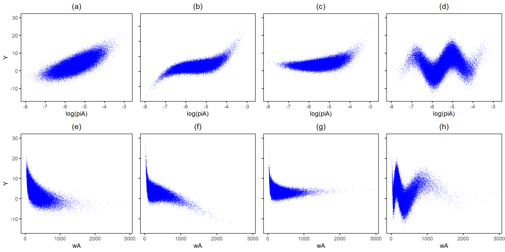
Figure 1: The proposed relationships between the outcome variable $Y$ and $log(\pi^{A})$ in $U$ for (a) $LIN$, (b) $CUB$, (c) $EXP$ and (d) $SIN$ scenarios, and between the outcome $Y$ and sampling weights $w^{A}$ for (e) $LIN$, (f) $CUB$, (g) $EXP$ and (h) $SIN$ scenarios.

We then consider an informative sampling strategy with unequal probabilities of inclusion, where the selection mechanism of $S_{A}$ and $S_{R}$ depends on $x$ and $d$, respectively. Thus, each $i\in U$ is assigned two values within $(0,1)$ corresponding to the probabilities of selection in $S_{R}$ and $S_{A}$ through a $logistic$ function as below:

$$\pi^{R}(d_{i})=p(\delta^{R}_{i}=1|d_{i}) =\frac{exp\{\gamma_{0}-0.4d_{i}\}}{1+exp\{\gamma_{0}-0.4d_{i}\}}$$ (3.13)

$$\pi^{A}(x_{i})=p(\delta^{A}_{i}=1|x_{i}) =\frac{exp\{\gamma_{1}+\gamma_{2}x_{i}\}}{1+exp\{\gamma_{1}+\gamma_{2}x_{i}\}}$$ (3.14)

where $\delta^{R}_{i}$ and $\delta^{A}_{i}$ are the indicators of being selected in $S_{R}$ and $S_{A}$, respectively, for $i\in U$. we initially set $\gamma_{2}=0.3$, which yields PS with a normal range. To assess how the adjustments behave in presence of influential weights, later we set $\gamma_{2}=0.6$, which yields relatively extreme weights.

Associated with $S_{R}$ and $S_{A}$, independent samples of expected sizes $n_{R}=1,000$ and $n_{A}=500$ are selected randomly from $U$ with a Poisson sampling design. We choose $n_{A}<n_{R}$ as is the case in the two applications of this study. The model intercepts, $\gamma_{0}$ and $\gamma_{1}$ in 3.13, are obtained such that $\sum_{i=1}^{N}\pi^{R}_{i}=n_{R}$ and $\sum_{i=1}^{N}\pi^{A}_{i}=n_{A}$, respectively. The rest of the simulation design is similar to that defined in Simulation I, except for the way we specify a working model. A QR model is misspecified by replacing $x_{i}$ with $x^{2}_{i}$, and a PM model is misspecified by replacing $f_{k}(x_{i})$ with $x^{2}_{i}$ and $d_{i}$ with $d^{2}_{i}$, and also by dropping the interaction term $x_{i}d_{i}$.

3.2.2 Results

Figure 2 compares the relative bias (rBias) magnitude and efficiency of the competing methods for the continuous outcome variable, $y^{c}$, across different scenarios of model specification while $\gamma_{2}=0.3$. Note that the error bars reflect the relative length of 95% CIs (rlCI). As illustrated, point estimates from both $S_{R}$ and $S_{A}$ are biased if the sampling true weights are ignored. At the first glance, one can infer that for all $f_{k}$, $k=1,2,3,4$, the magnitude of rBias is close to $zero$ as long as either QR or PM model is valid. However, in situations where $\pi^{A}$ is non-linearly associated with $y^{c}$, i.e. plots (b), (c), and (d), the AIPW and PAPP estimators are biased when the PM is misspecified, but the QR model is valid. In contrast, the LWP method yields slightly biased estimates in all plots when the QR model is misspecified, but the PM is correct. It turns out that the GPPP is the only method that leads to unbiased estimates in all the scenarios with respect to model specification and functional form of the PM. We did not observe consistent results across the adjustment methods with respect to efficiency. However, the GPPP method consistently shows high efficiency compared to the other methods across all the studied scenarios.

We summarize the simulation results for the binary outcome, $y^{b}$, with $\gamma_{2}=0.3$ in Figure 3. Again, adjusted estimates are unbiased if the working model for either QR or PM holds. Exceptions are seen for the PAPP and AIPW methods with residual bias in the plots related to (c) EXP, and (d) SIN when the PM is incorrectly specified. Unlike the simulation results for the continuous variable, the LWP consistently produces unbiased estimates for the binary outcome when the working model for QR fails. However, the magnitude of bias seems to be much larger in the LWP method when both underlying models for QR and PM are misspecified. Again, as for the continuous outcome, the proposed GPPP method consistently gives unbiased and efficient estimates. The lowest efficiency is associated with the AIPW and PAPP methods in the EXP scenario when the PM is misspecified.

Figure 4 displays the results of crCI and rSE for the continuous outcomes where $\gamma_{2}=0.3$. According to the rSE values, all methods perform well in variance estimation except for the LWP method which consistently underestimates the variance. A similar problem appears in the PAPP and AIPW methods for the EXP scenario when the outcome model is invalid. Generally, the Bayesian methods, i.e. GPPP and LWP, tend to slightly overestimate the variance. The values of crCI seem to be close to the nominal level for all the methods across almost all the scenarios, as long as at least one of the underlying models holds. For the non-linear associations, i.e. (b) CUB, (c) EXP and (d) SIN, the 95% CIs associated with frequentist methods, i.e. AIPW and PAPP, tend to undercover the population mean when the outcome model is false. Figure 5 depicts similar results for the binary outcome when $\gamma_{2}=0.3$. Overall, the results look analogous to those obtained for the continuous outcome. However, the degree of overestimation of variance by the Bayesian methods seems to be larger in the binary outcome than the continuous outcome.

Extensions of the simulation for other sample size combinations, i.e. $(n_{A},n_{R})=(500,500)$ and $(n_{A},n_{R})=(1,000,500)$ and also for $\gamma_{2}=0.6$, which creates extreme sampling weights in $S_{A}$, are included in Appendix 8.2. While we observe no major discrepancy in the simulation results for other sample size scenarios than $(n_{A},n_{R})=(500,1,000)$, having influential weights presented in $S_{A}$ leads to a larger magnitude of bias and lower efficiency in the estimates of PAPP, AIPW when the PM is incorrectly specified, but the QR model is valid. However, the GPPP method seems to be least affected by the presence of extreme weights.

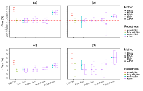
Figure 2: Comparing the performance of the adjusted estimators under different model-specification scenarios for the continuous outcome variable with $\gamma_{2}=0.3$ under (a) $LIN$, (b) $CUB$, (c) $EXP$, and (d) $SIN$ scenarios. The error bars have been drawn based on the 2.5% and 97.5% percentiles of the empirical distribution of bias over the simulation iterations. UW: unweighted; FW: Fully weighted; PAPP: Propensity-adjusted Probability Prediction; GPPP: Gaussian Processes of Propensity Prediction; LWP: Linear-in-weight Prediction; AIPW: Augmented Inverse Propensity Weighting

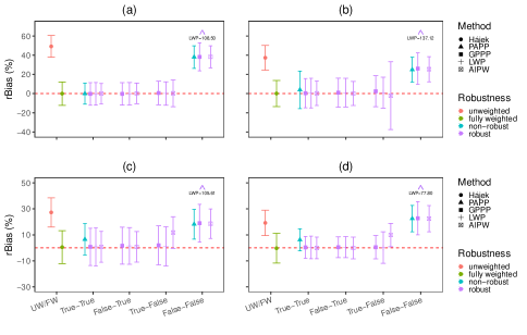
Figure 3: Comparing the performance of the adjusted estimators under different model-specification scenarios for the binary outcome variable with $\gamma_{2}=0.3$ under (a) $LIN$, (b) $CUB$, (c) $EXP$, and (d) $SIN$ scenarios. The error bars have been drawn based on the 2.5% and 97.5% percentiles of the empirical distribution of bias over the simulation iterations. UW: unweighted; FW: Fully weighted; PAPP: Propensity-adjusted Probability Prediction; GPPP: Gaussian Processes of Propensity Prediction; LWP: Linear-in-weight Prediction; AIPW: Augmented Inverse Propensity Weighting

In Figures 4 and 5, we depict the measures associated with the accuracy of the variance methods for GPPP/AIPW estimators. One can immediately infer that for both employed methods, the variance estimator is approximately unbiased when at least one of the underlying models holds. However, in situations where both models are invalid, according to the rSE values, the AIPW estimator tends to underestimate/overestimate the variance to a significant extent, while the variance estimator under GPPP shows more robustness across the model specification scenarios as well as outcome variables. Last but not least, the proximity of the crCI values to $95\%$ for the GPPP methods, especially when both underlying models are wrong, reflects the accuracy of both point and variance estimates under the GPPP method.

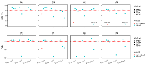
Figure 4: Comparing the 95% CI coverage rates (crCI) of the DR adjusted means for the continuous outcome variable with $\gamma_{2}=0.3$ under (a) $LIN$, (b) $CUB$, (c) $EXP$, and (d) $SIN$ scenarios, and SE ratios (rSE) under (e) $LIN$, (f) $CUB$, (g) $EXP$, and (h) $SIN$ scenarios, across different DR methods under different model specification scenarios. UW: unweighted; FW: Fully weighted; PAPP: Propensity-adjusted Probability Prediction; GPPP: Gaussian Processes of Propensity Prediction; LWP: Linear-in-weight Prediction; AIPW: Augmented Inverse Propensity Weighting

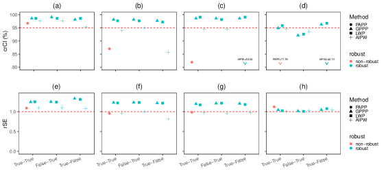
Figure 5: Comparing the 95% CI coverage rates (crCI) of the DR adjusted means for the binary outcome variable with $\gamma_{2}=0.3$ under (a) $LIN$, (b) $CUB$, (c) $EXP$, and (d) $SIN$ scenarios, and SE ratios (rSE) under (e) $LIN$, (f) $CUB$, (g) $EXP$, and (h) $SIN$ scenarios, across different DR methods under different model specification scenarios. UW: unweighted; FW: Fully weighted; PAPP: Propensity-adjusted Probability Prediction; GPPP: Gaussian Processes of Propensity Prediction; LWP: Linear-in-weight Prediction; AIPW: Augmented Inverse Propensity Weighting

So far, the results we discussed were limited to a case where $\rho=0.5$. As the final step, we replicate the simulation for different values of $\rho$ ranging from $0$ to $0.9$ to show how stable the competing methods perform in terms of rbias and rMSE. Figure 6 depicts changes in the values of rBias and rMSE in the continuous outcome, $y^{c}$, for different adjustment methods and across different model specification scenarios as the value of $\rho$ increases. Generally, it seems that the values of rBias and rMSE decline for all competing methods with an increase in $\rho$. In addition, for all values of $\rho$, it is evident that the GPPP method outperforms the PAPP, AIPW, LWP methods when the outcome model is wrong. This strength in GPPP is more evident when the association between the outcome and the PS is non-linear, i.e. in (b) CUB, (c) EXP, and (d) SIN. In Figure 7, we display corresponding comparisons for the binary outcome. The results are similar to those based on the continuous outcome, with a difference in that the values of rMSE increase with an increase in the value of $\rho$. Detailed numerical results of Simulation II is available in Appendix 8.2.

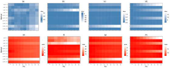
Figure 6: Comparing the magnitude of rBias of the DR adjusted means for the continuous outcome variable with $\gamma_{2}=0.3$ under (a) $LIN$, (b) $CUB$, (c) $EXP$, and (d) $SIN$, and rMSE under (e) $LIN$, (f) $CUB$, (g) $EXP$, and (h) SIN across different model specification scenarios and different values of $\rho$. UW: unweighted; FW: Fully weighted; PAPP: Propensity-adjusted Probability Prediction; GPPP: Gaussian Processes of Propensity Prediction; LWP: Linear-in-weight Prediction; AIPW: Augmented Inverse Propensity Weighting

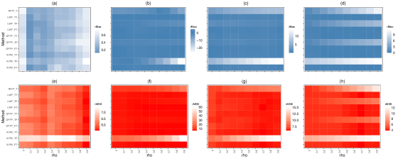
Figure 7: Comparing the magnitude of rBias of the DR adjusted means for the binary outcome variable with $\gamma_{2}=0.3$ under (a) $LIN$, (b) $CUB$, (c) $EXP$, and (d) $SIN$, and rMSE under (e) $LIN$, (f) $CUB$, (g) $EXP$, and (h) SIN across different model specification scenarios and different values of $\rho$. UW: unweighted; FW: Fully weighted; PAPP: Propensity-adjusted Probability Prediction; GPPP: Gaussian Processes of Propensity Prediction; LWP: Linear-in-weight Prediction; AIPW: Augmented Inverse Propensity Weighting

4 Applications

As the application part, we conduct an empirical study involving inference for a non-probability sample. Our goal is to estimate police-reportable crash rates per 100M miles driven using the sensor-based data from the second phase of the Strategic Highway Research Program (SHRP2). To this end, we consider the National Household Travel Survey (NHTS) 2017 as the reference survey to adjust for the potential selection bias in crash rates. The following two subsections briefly describe the design of these samples and discuss the findings in detail.

4.1 Strategic Highway Research Program 2

SHRP2 is the largest naturalistic driving study (NDS) conducted to date, with the primary aim to assess how people interact with their vehicle and traffic conditions while driving (SHRP2, 2013). About $A=3,140$ drivers aged $16-95$ years were recruited from six geographically dispersed sites across the United States, and over five million trips and $50$ million driven miles have been recorded during their participation time. The average follow-up time per person was $440$ days. A quasi-random approach was initially employed to select samples by random cold calling from a pool of $17,000$ pre-registered volunteers. However, because of the low success rate along with budgetary constraints, the investigators later chose to pursue voluntary recruitment. Sites were assigned one of three pre-determined sample sizes according to their population density (Campbell, 2012). The youngest and eldest age groups were oversampled in the sense that crash risk is expected to be higher among those subgroups. Thus, one can conclude that the selection mechanism in SHRP2 is a combination of convenience and quota sampling methods. Further description of the study design and recruitment process can be found in Antin et al. (2015).

SHRP2 data are collected in multiple stages. Selected participants are initially asked to complete multiple assessment tests, including executive function and cognition, visual perception, visual-cognitive, physical and psychomotor capabilities, personality factors, sleep-related factors, general medical condition, driving knowledge, etc. In addition, demographic information such as age, gender, household income, education level, and marital status as well as vehicle characteristics such as vehicle type, model year, manufacturer, and annual mileage are gathered at the screening stage. A trip in SHRP2 is defined as the time interval during which the vehicle is operating. The in-vehicle sensors start recording kinematic information, the driver’s behaviors, and traffic events continuously as soon as the vehicle is switched on. Encrypted data are stored in a removable hard drive, and participants are asked to provide access to the vehicle every four to six months, so that hard drives with accumulated data are removed and replaced. Then, trip-related information such as average speed, duration, distance, and GPS trajectory coordinates are obtained by aggregating the sensor records at the trip level (Antin et al., 2019; Campbell, 2012).

4.2 National Household Travel Survey 2017

In the present study, we use data from the eighth round of the NHTS conducted from March 2016 through May 2017 as the reference survey. The NHTS is a nationally representative survey, repeated cross-sectionally almost every seven years. It is aimed at characterizing personal travel behaviors among the civilian, non-institutionalized population of the United States. The 2017 NHTS was a mixed-mode survey, in which households were initially recruited by mailing through an address-based sampling (ABS) technique. Within the selected households, all eligible individuals aged $\geq 5$ years were requested to report the trips they made on a randomly assigned weekday through a web-based travel log. Proxy interviews were requested for younger household members who were $\leq 15$ years old.

The overall sample size was $129,696$, of which roughly $20$% was used for national representativity and the remaining $80$% was regarded as add-ons for the state-level analysis. The recruitment response rate was $30.4$%, of which $51.4$% reported their trips via the travel logs (Santos et al., 2011). In NHTS, a travel day is defined from $4:00$ AM of the assigned day to $3:59$ AM of the following day on a typical weekday. A trip is defined as that made by one person using any mode of transportation. While trip distance was measured by online geocoding, the rest of the trip-related information was based on self-reporting. A total of $264,234$ eligible individuals aged $\geq$5 took part in the study, for which $923,572$ trips were recorded (McGuckin and Fucci, 2018).

4.3 Auxiliary variables and analysis plan

Our focus here was on inference at the participant level, so both SHRP2 and NHTS data were aggregated. Considering this, we calculated the total distance driven and total number of police-reported crashes for each participant of SHRP2. The total of these quantities by all SHRP2 participants were $28$M miles and $210$, respectively. To make the two datasets more comparable, we also filtered out all the subjects in NHTS who were not drivers or were younger than $16$ years old or used public transportation or transportation modes other than cars, SUVs, vans, or light pickup trucks. In addition, we restricted the NHTS sample to those respondents who reside in the SHRP2-specific six states, so our inferences are only generalizable to those six states. The final sample sizes of the complete datasets were $n_{A}=2,862$ and $n_{R}=29,572$ in SHRP2 and NHTS, respectively.

To address the expressed objective of the present study, we set the outcome variable to be the frequency of police-reported crashes by SHRP2 participants throughout their follow-up time. In addition, we utilize the total miles driven by each SHRP2 participant as the model offset to obtain the rates by a driven mile. Particular attention was paid to identify as many relevant common auxiliary variables as possible in the combined sample that are expected to govern both selection mechanism and response surface in SHRP2. Two distinct sets of variables were considered: (i) demographic and socio-economic information of the drivers including sex, age groups, race, ethnicity, birth country, education level, household size, number of owned vehicles, and state of residence, and (ii) vehicle characteristics including vehicle age, vehicle manufacturer, vehicle type and fuel type.

We chose to use a Bayesian negative binomial (NB) regression for modeling the response surface because the outcome variable was count data and effects of overdispersion were present. The log of the total miles driven by SHRP2 participants is included as offset in the model such that crash rates can be predicted by unit of distance driven. conditional on $x_{i}$ and $\widehat{\pi}^{i}_{i}$, the outcome model is given by

$$y_{i}|x_{i},t_{i},\theta,\phi,\gamma,\alpha,\tau,\sigma\sim NB\left(exp\big{\{}\theta_{0}+x_{i}^{T}\theta_{1}+f\left(x^{T}_{A}(\phi-\gamma),\alpha,\rho,\tau\right)+log(t_{i})\big{\}},1/\sigma\right)$$ (4.1)

where $t_{i}$ is the total distance driven by respondent $i$, and $\sigma\sim Cauchy^{+}(0,3)$. Note that we also checked and found no evidence of zero-inflation in the distribution of the outcome by comparing the observed zeros with the expected number of zeros under the proposed NB model.

4.3.1 Results

According to Figure 8, one can visually infer that the largest discrepancies between the sample distribution of auxiliary variables in SHRP2 and that in the population stem from participants’ age, race, and population size of the residential area as well as vehicles’ age and vehicles’ type. The youngest and oldest age groups are overrepresented as are Whites and non-Hispanics. In addition, we found that the proportion of urban dwellers is higher in SHRP2 than that in the NHTS. In terms of vehicle characteristics, SHRP2 participants tend to own passenger cars more than the population average, whereas individuals with other vehicle types were underrepresented in SHRP2.

Before any attempt for bias adjustment, we check the positivity assumption as well as the existence of influential pseudo-weights. To this end, we estimate the pseudo-selection probabilities for the units of the SHRP2 sample using the PAPP method as well as the PMLE method by Wang et al. (2020). Figure 9a compares the distribution of estimated PS in log scale between the SHRP2 and NHTS samples. As illustrated, there is a slight lack of common support in the distribution of PS, which may lead to extreme weights. The box-plot on the right side (Figure 9b) confirms the presence of outlying pseudo-weights based on the PAPP method. However, it seems no outliers exist in the pseudo-weights based on the PMLE method. Figure 10 compares the distribution of auxiliary variables between the two samples after (pseudo-)weighting. As illustrated, pseudo-weighting obviates most of the previously seen discrepancies in the distribution of common covariates.

Figure 11 displays the adjusted estimates of police-reported crash rates per 100M miles driven and associated 95% CIs using the LWP and GPPP methods by age groups. The plot also compares the adjusted estimates in SHRP2/NHTS data with the naive estimate using SHRP2-only data and that based on the GES/ADS data, which is here considered as the benchmark Tefft (2017). Note that the latter represents the entire population of American drivers while our adjusted estimates represent the SHRP2 target population. As illustrated, for most of the age groups, adjustments shift the unweighted crash rates to the true population value, and the associated 95% CIs overlap, except for the last age group, i.e $80+$ years old. In particular, the unweighted crash rate for the age group 50-59 years seems to be severely biased while adjusted estimates are desirably close to the true population value. While we observe no significant differences in the performance of the GPPP and LWP methods, it is evident that GPPP offers more efficient estimates than the LWP method, as the length of 95% CIs is consistently lower in GPPP than LWP. Finally, one can infer from Figure 11 that the risk of traffic accidents is higher among young and elder people.

In Figure 12, we assess the adjusted rates of police-reportable crashes across levels of auxiliary variables. The major associations we observe are as follows: Whites, more educated drivers, and those in middle-income families are at lower risk of traffic accidents. In addition, there is a positive relationship between the crash risk and household size. There is also evidence of higher crash rates among Vans, European, and gas/diesel vehicles. Numerical values associated with this plot have been provided in Table 16 of Appendix 8.3.

Figure 8: Comparing the distribution of common auxiliary variables in SHRP2 with weighted NHTS

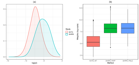
Figure 9: Comparing the empirical density of (a) estimated propensity scores between SHRP2 and NHTS and (b) estimated pseudo-weights in SHRP2 across the applied quasi-randomization methods

Figure 10: Comparing the distribution of common auxiliary variables in pseudo-weighted SHRP2 based on the PAPP method with weighted NHTS

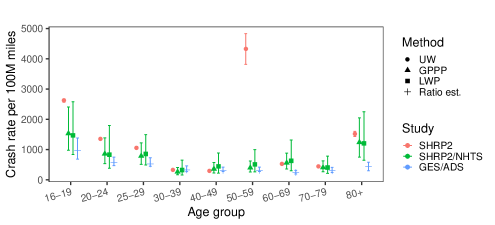
Figure 11: Comparing the performance of adjustment methods for estimating crash rates per 100M miles and associated 95% CIs in SHRP2/NHTS with native estimates and those based on CES/ADS as benchmark across age groups. UW: unweighted; FW: Fully weighted; PAPP: Propensity-adjusted Probability Prediction; GPPP: Gaussian Processes of Propensity Prediction; LWP: Linear-in-weight Prediction.

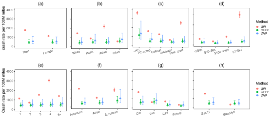
Figure 12: Comparing the performance of adjustment methods for estimating crash rates per 100M miles and associated 95% CIs in SHRP2/NHTS with native estimates across levels of (a) sex, (b) race, (c) education, (d) household income, (e) household size, (f) vehicle make, (g) vehicle type, and (d) fuel type. UW: unweighted; GPPP: Gaussian Process of Propensity Prediction; LWP: Linear-in-weight Prediction.

5 Discussion

In the present article, we proposed alternative methods for inference based non-probability samples with the goal to fill some of the gaps in the current literature. To our knowledge, this was the first study proposing a fully Bayesian method in a non-probability sample setting that jointly estimates the PS and outcome, and allows one to directly simulate the posterior predictive distribution of the population quantity under a non-probability sample setting. Bayesian approaches provide a unified framework for deriving the variance of the point estimator by simulating the posterior predictive distribution of the population unknown parameters. A well-calibrated Bayesian method can appropriately capture all sources of uncertainty, and therefore, yields desirable frequentist repeated sampling properties (Dawid, 1982). Unlike the Bayesian two-step methods (Kaplan and Chen, 2012; Rafei et al., 2021), it is well-understood that joint modeling of the PS and the outcome, as was the case in this article, results in accurate variance estimation (Little, 2004).

The alternative design-based approaches, such as the AIPW estimator, are sensitive to the presence of influential pseudo-weights if the outcome model is invalid. In addition, the variance estimator proposed by Chen et al. (2019) relies on asymptotic theory, and there is no guarantee that simultaneously solving the estimating leads to a unique set of solutions. As another major limitation, such a method works only when the auxiliary variables are identical in the QR and PM models. According to the likelihood we factorized in Eq. 2.1, the dimension of the auxiliary variables may vary across the QR and PM methods in a non-probability sample setting ($\{X,D\}$ vs $X$), which makes it impossible to use Chen’s AIPW method in practice. On the other hand, employing a fully model-based approach can be extremely expensive computationally, as one has to fit the propensity model on a synthesized population, and predict the outcome variable for its entire non-sampled units Little and Zheng (2007); Mercer (2018). However, the method we proposed requires fitting the model only on the combined sample, which makes it computationally more parsimonious, especially in a Big Data setting.

The results of our simulation studies reveal that the proposed GPPP method is doubly robust in terms of both point and variance estimates. Furthermore, estimates based on the GPPP method were more efficient than those based on the LWP method especially when outlying pseudo-weights are present and the PM is misspecified. We also showed that the use of GP with a stationary isotropic covariance structure provides a stronger rationale than Spline in the PSPP method as it is equivalent to a non-parametric matching technique based on the estimated PS (Huang et al., 2019). While Bayesian joint modeling demonstrates good frequentist properties, feedback occurs between the two models (Zigler et al., 2013). This can be controversial in the sense that PS estimates should not be informed by the outcome model (Rubin, 2007).

It is worth noting that although our proposed method limited computations to the combined samples, Bayesian joint modeling can still turn out computationally very expensive, even using the low-rank approximation techniques. To conduct the simulation studies of this research, we had to hire high-performance computing servers to be able to do parallel processing, but these resources are costly to hire and may not be available for every researcher. Finally, we want to pinpoint that our proposed estimator still contains a design-based term, and therefore, adjusted estimates can still be inefficient if there are extreme values in the sampling weights of $S_{R}$. However, this should not be of a big concern compared to the pseudo-weights of $S_{A}$ as $S_{R}$ is supposed to be a well-designed probability sample. As discussed earlier, a fully model-based estimator will require generating synthetic populations which cannot be fully implemented on the current Bayesian platforms.

6 Acknowledgement

The present study was part of the doctoral research of the first author of this article at the Michigan Program in Survey and Data Science. Therefore, we would like to thank the respected members of the dissertation committee, Professors Brady T. West, Roderick J. Little, and Philip S. Boonstra at the University of Michigan, who have continuously supported this research with their excellent comments and critical feedback. Our gratitude also goes to Professors Katharine Abraham, Stanley Presser, and Joseph Sedarski at the University of Maryland who have significantly contributed to the development of the main idea of this paper with their valuable comments and feedback over the doctoral seminar course. Last but not least, the authors would like to thank all the researchers and staff who have been involved in collecting the data of SHRP2 and NHTS.

7 Conflict of Interest

The authors declare that there was no conflict of interest in the current research.

8 Appendix

8.1 Gaussian Processes and kernel weighting

Suppose $\widehat{\pi}^{A}_{i}$ is the estimated PS for $i\in S_{A}$ based on a pseudo-weighting approach. Consider the following Gaussian Process (GP) regression model:

$$y_{i}=f(u_{i})+\epsilon_{i}$$ (8.1)

where $u_{i}=log(\widehat{\pi}^{A}_{i})$, and $f\sim Gp(0,K)$ with $K(u_{i},u_{j};\alpha,\rho)=Cov\left(f(u_{i}),f(u_{j})\right)$. From a weight-space viewpoint, one can show that the model 8.1 predicts $y_{i}$ for $i\in S_{R}$ using a weighted sum of observed $y_{i}$ in $S_{A}$ as below:

$$\widehat{y}_{i}=\sum_{j=1}^{n_{A}}\widetilde{w}_{ij}y_{j}$$ (8.2)

where

$$\widetilde{w}_{ij}=\frac{k_{ij}}{\sum_{j=1}^{n_{A}}k_{ij}}\hskip 14.22636ptand\hskip 14.22636ptk_{ij}=k^{T}(u_{j})\Sigma^{-1}$$ (8.3)

with $k(\widehat{\pi}^{A}_{j})=k(\widehat{\pi}^{A}_{j},\widehat{\pi}^{A}_{i})_{n_{A}\times 1}$. According to Huang et al. (2019), $\widehat{y}_{i}$ can be regarded as the Nadaraya-Watson estimator of the observed outcome and selection indicator in the population.

Considering an isotropic covariance structure, which is a function of $||u_{j}-u_{i}||$, $k_{ij}$ quite resembles the kernel weights Wang et al. (2020), with the bandwidth $h$ equivalent to the GP length-scale parameter $\rho$. Since the kernel weights obtained by GP is used in the PM estimator, it is clear that the final weights will be multiplied by $w^{R}$, i.e.

$$\widehat{w}_{j}=\sum_{i=1}^{n_{R}}k_{ij}w^{R}_{i}$$ (8.4)

One can show that the major kernel-related condition determined by Wang et al. (2020) to obtain consistency in the kernel-weighted estimates holds for a Matérn family covariance structure, i.e. $K(u)$, $\int K(u)du=1$, $Sup_{u}|K(u)|<\infty$, and $lim_{|u|\rightarrow\infty}|u||K(u)|=0$.

8.2 Further extensions of the simulation study

8.2.1 Simulation study I

This subsection provides additional results associated with Simulation I. Table 2 and Table 3 summarize the findings of the simulation in Section 3.1 for $\rho=0.5$ and $\rho=0.3$, respectively.

Table 2: Comparing the performance of the bias adjustment methods in the first simulation study for $\rho=0.5$

	$n_{A}=500,\hskip 5.69054ptn_{R}=500$					$n_{A}=1,000,\hskip 5.69054ptn_{R}=500$					$n_{A}=500,\hskip 5.69054ptn_{R}=1,000$
Measure	rBias	rMSE	crCI	lCI	rSE	rBias	rMSE	crCI	lCI	rSE	rBias	rMSE	crCI	lCI	rSE
Probability sample ($S_{R}$)
UW	8.866	9.445	21.759	1.149	0.965	8.866	9.445	21.759	1.149	0.965	8.810	9.115	2.778	0.816	0.954
FW	0.260	3.770	93.056	1.363	0.991	0.260	3.770	93.056	1.363	0.991	0.080	2.736	95.833	0.967	0.967
Non-probability sample ($S_{A}$)
UW	30.708	30.926	0.000	1.304	0.974	30.008	30.104	0.000	0.916	1.039	30.708	30.926	0.000	1.304	0.974
FW	-0.134	3.763	93.981	1.363	0.991	-0.146	2.659	95.833	0.957	0.986	-0.134	3.763	93.981	1.363	0.991
Model specification: QR–True, PM–True
GPPP	0.129	3.876	99.537	1.912	1.350	0.000	3.055	99.537	1.724	1.544	0.092	3.567	98.148	1.576	1.209
LWP	-0.063	4.200	99.537	2.516	1.638	-0.145	3.140	99.537	1.737	1.514	-0.135	3.742	97.685	1.613	1.179
AIPW	-0.101	4.035	93.981	1.406	0.953	-0.098	3.139	94.907	1.107	0.965	-0.232	3.760	94.907	1.311	0.955
PAPP	0.832	4.012	93.056	1.406	0.980	0.547	2.998	93.981	1.078	1.000	0.984	3.844	95.370	1.339	0.985
Model specification: QR–True, PM–False
GPPP	0.146	3.829	99.537	1.903	1.360	-0.017	3.068	99.537	1.720	1.533	0.161	3.555	98.148	1.575	1.213
LWP	-0.007	3.876	99.537	1.910	1.348	-0.124	3.084	99.537	1.730	1.535	-0.015	3.575	98.148	1.585	1.213
AIPW	-0.056	3.916	94.907	1.358	0.948	-0.087	3.061	95.833	1.070	0.957	-0.180	3.590	93.981	1.272	0.970
Model specification: QR–False, PM–True
GPPP	1.317	4.321	99.074	1.934	1.285	1.146	3.477	99.537	1.748	1.456	1.314	4.001	96.296	1.607	1.163
LWP	4.052	6.752	89.815	2.236	1.132	4.147	6.026	92.130	2.004	1.253	4.090	6.299	87.037	1.850	1.056
AIPW	0.040	3.987	95.833	1.392	0.954	-0.010	3.025	94.444	1.074	0.971	0.073	3.716	93.519	1.338	0.984
Model specification: QR–False, PM–False
GPPP	27.400	27.678	0.000	2.239	1.564	26.595	26.733	0.000	2.042	2.055	27.430	27.692	0.000	1.814	1.306
LWP	27.075	27.361	0.000	2.247	1.558	26.434	26.575	0.000	2.056	2.053	27.127	27.395	0.000	1.837	1.314
AIPW	27.115	27.402	0.000	1.366	0.944	26.432	26.571	0.000	0.981	0.987	27.056	27.328	0.000	1.334	0.949
PAPP	27.912	28.191	0.000	1.354	0.936	27.024	27.158	0.000	0.968	0.983	28.121	28.381	0.000	1.329	0.950

• GPPP: Gaussian Process of Propensity Prediction; LWP: Linear-in-weight prediction; AIPW: Augmented Inverse Propensity Weighting; PAPP: Propensity-adjusted Probability Prediction
  NOTE: The PAPP and AIPW methods have been implemented through a bootstrap method.

Table 3: Comparing the performance of the bias adjustment methods in the first simulation study for $\rho=0.3$

	$n_{A}=500,\hskip 5.69054ptn_{R}=500$					$n_{A}=1,000,\hskip 5.69054ptn_{R}=500$					$n_{A}=500,\hskip 5.69054ptn_{R}=1,000$
Measure	rBias	rMSE	crCI	lCI	rSE	rBias	rMSE	crCI	lCI	rSE	rBias	rMSE	crCI	lCI	rSE
Probability sample ($S_{R}$)
UW	8.867	10.406	58.796	1.927	0.965	8.867	10.406	58.796	1.927	0.965	8.797	9.612	38.889	1.369	0.964
FW	0.424	6.361	92.593	2.303	0.989	0.424	6.361	92.593	2.303	0.989	0.154	4.580	95.370	1.633	0.973
Non-probability sample ($S_{A}$)
UW	30.759	31.251	0.000	2.037	1.006	30.082	30.322	0.000	1.435	1.028	30.759	31.251	0.000	2.037	1.006
FW	-0.277	6.284	95.833	2.335	1.014	-0.298	4.529	93.519	1.639	0.989	-0.277	6.284	95.833	2.335	1.014
Model specification: QR–True, PM–True
GPPP	0.438	6.297	100.000	3.413	1.482	0.061	4.754	99.537	3.094	1.775	0.489	6.052	99.074	2.821	1.275
LWP	-0.342	6.811	100.000	4.061	1.628	-0.266	4.917	99.537	3.131	1.739	-0.232	6.429	98.148	2.932	1.244
AIPW	-0.390	6.666	95.370	2.378	0.975	-0.296	4.911	94.444	1.737	0.966	-0.395	6.337	95.370	2.328	1.004
PAPP	0.574	6.537	95.370	2.366	0.991	0.360	4.696	95.370	1.709	0.995	0.873	6.291	94.907	2.334	1.022
Model specification: QR–True, PM–False
GPPP	0.553	6.241	100.000	3.391	1.488	0.077	4.733	99.537	3.080	1.775	0.585	6.033	98.611	2.817	1.280
LWP	-0.115	6.302	100.000	3.464	1.499	-0.255	4.748	99.537	3.105	1.786	-0.020	6.114	99.074	2.879	1.284
AIPW	-0.271	6.301	95.370	2.312	1.002	-0.275	4.789	94.444	1.688	0.963	-0.287	6.042	94.907	2.233	1.009
Model specification: QR–False, PM–True
GPPP	1.891	6.750	99.537	3.409	1.435	1.372	5.092	99.537	3.097	1.722	1.981	6.536	97.685	2.837	1.242
LWP	4.179	8.638	98.611	3.692	1.332	4.373	7.326	99.537	3.309	1.535	4.277	8.280	95.833	3.098	1.192
AIPW	-0.146	6.594	94.907	2.377	0.983	-0.187	4.794	94.444	1.708	0.973	-0.125	6.319	95.370	2.333	1.007
Model specification: QR–False, PM–False
GPPP	27.642	28.234	5.093	3.483	1.652	26.734	27.051	2.315	3.212	2.121	27.792	28.364	0.463	2.792	1.344
LWP	26.915	27.545	11.111	3.542	1.649	26.278	26.601	2.315	3.242	2.142	27.022	27.636	1.852	2.900	1.366
AIPW	26.987	27.603	0.000	2.120	0.997	26.405	26.734	0.000	1.528	0.996	27.022	27.630	0.000	2.076	0.982
PAPP	27.881	28.473	0.000	2.122	1.002	26.994	27.300	0.000	1.501	1.004	28.146	28.716	0.000	2.104	1.008

• GPPP: Gaussian Process of Propensity Prediction; LWP: Linear-in-weight prediction; AIPW: Augmented Inverse Propensity Weighting; PAPP: Propensity-adjusted Probability Prediction
  NOTE: The PAPP and AIPW methods have been implemented through a bootstrap method.

8.2.2 Simulation study II

Table 4 exhibits the numerical results associated with Figure 2 and Figure 3. $LIN$ $CUB$ $EXP$ $SIN$ Measure rBias rMSE crCI lCI rSE rBias rMSE crCI lCI rSE rBias rMSE crCI lCI rSE rBias rMSE crCI lCI rSE Probability sample ($S_{R}$) UW -23.870 24.078 0.000 12.411 1.001 -17.120 17.243 0.000 8.442 1.045 -12.097 12.179 0.000 5.427 0.976 -18.475 19.159 3.241 18.535 0.93 FW -0.180 3.921 93.519 15.087 0.980 -0.156 2.749 94.907 10.799 1.001 -0.091 1.947 94.444 7.392 0.967 0.015 5.549 93.519 20.503 0.94 Non-probability sample ($S_{A}$) UW 48.795 49.086 0.000 19.644 0.936 30.073 30.366 0.000 15.989 0.966 18.146 18.363 0.000 10.710 0.969 27.948 28.716 0.926 25.807 0.995 FW -0.178 6.184 91.204 22.458 0.925 -0.218 4.249 92.593 15.612 0.936 0.004 2.282 93.981 8.639 0.964 -0.034 8.276 93.519 31.425 0.966 Non-robust method Model specification: QR–True PAPP 0.066 4.771 95.370 19.982 1.066 -7.545 24.919 91.667 53.569 0.574 2.269 3.182 83.333 8.794 1.003 11.642 13.063 46.759 23.010 0.988 Model specification: QR–False PAPP 35.346 35.660 0.000 17.238 0.929 17.490 17.760 0.000 11.878 0.980 10.111 10.362 0.000 8.707 0.977 30.831 31.610 0.463 26.668 0.973 Doubly robust methods Model specification: QR–True, PM–True GPPP 0.025 4.439 98.148 18.703 1.081 -0.060 3.150 96.759 13.124 1.067 -0.027 2.164 97.222 8.823 1.048 0.301 6.250 96.296 26.369 1.084 LWP -0.038 4.478 97.222 18.960 1.088 -0.005 3.133 98.148 13.227 1.084 -2.254 4.458 95.833 9.065 0.080 0.299 6.335 96.296 26.621 1.076 AIPW 0.000 4.439 97.222 18.266 1.047 0.250 4.060 98.148 16.137 1.014 -0.022 2.194 93.981 8.482 0.984 0.157 6.179 94.444 23.568 0.971 Model specification: QR–True, PM–False GPPP 0.099 4.467 97.685 18.732 1.078 -0.061 3.136 97.222 12.796 1.047 0.005 2.140 96.296 8.654 1.037 0.439 6.189 95.833 25.041 1.043 LWP 10.099 4.776 91.667 17.809 0.100 7.636 3.382 88.889 12.078 0.087 5.845 17.130 89.815 8.171 0.078 7.886 14.740 92.130 24.236 0.175 AIPW -0.033 4.608 94.907 18.233 1.007 -0.109 3.198 95.833 12.461 0.992 -0.048 2.188 95.370 8.400 0.977 0.245 6.221 94.907 23.752 0.972 Model specification: QR–False, PM–True GPPP 0.523 4.628 97.685 20.143 1.128 1.310 3.829 95.370 15.280 1.093 0.575 2.531 96.296 11.294 1.175 0.819 6.523 95.833 27.890 1.108 LWP -0.294 4.923 96.296 20.356 1.064 0.231 6.026 93.981 15.853 0.677 0.509 5.817 96.759 11.564 0.512 -1.060 14.048 92.130 37.060 0.679 AIPW 0.546 6.979 94.444 29.210 1.069 -15.872 46.090 87.500 102.060 0.600 6.885 7.391 26.389 10.549 0.999 14.490 15.884 35.648 24.548 0.96 Model specification: QR–False, PM–False GPPP 36.369 36.676 0.000 22.484 1.217 18.222 18.524 0.000 15.525 1.195 10.492 10.758 0.926 10.941 1.182 30.956 31.750 3.241 33.560 1.222 LWP 36.049 36.361 0.000 22.546 1.219 18.396 18.690 0.000 15.611 1.213 10.590 10.856 0.926 11.005 1.185 30.650 31.450 2.778 35.040 1.276 AIPW 36.146 36.468 0.000 17.448 0.919 18.293 18.583 0.000 12.436 0.967 10.587 10.848 0.000 8.968 0.965 30.664 31.483 0.000 26.807 0.956

• UW: Unweighted; FW: Fully weighted; GPPP: Gaussian Process of Propensity Prediction; LWP: Linear-in-weight prediction; AIPW: Augmented Inverse Propensity Weighting.
  NOTE: The PAPP and AIPW methods have been implemented through a bootstrap method.

Table 4: Comparing the performance of the bias adjustment methods in the second simulation study for the continuous outcome with $(n_{A},n_{R})=(500,1,000)$ and $\gamma_{1}=0.3$

Table 5: Comparing the performance of the bias adjustment methods in the second simulation study for the continuous outcome with $(n_{A},n_{R})=(1,000,500)$ and $\gamma_{1}=0.3$

	$LIN$					$CUB$					$EXP$					$SIN$
Measure	rBias	rMSE	crCI	lCI	rSE	rBias	rMSE	crCI	lCI	rSE	rBias	rMSE	crCI	lCI	rSE	rBias	rMSE	crCI	lCI	rSE
Probability sample ($S_{R}$)
UW	-23.868	24.297	0.000	17.587	0.985	-17.158	17.440	0.000	11.959	0.974	-12.107	12.274	0.000	7.683	0.967	-18.706	19.966	22.222	26.219	0.956
FW	0.118	5.477	93.519	21.395	0.994	0.016	3.998	94.444	15.257	0.971	0.015	2.673	95.833	10.454	0.995	-0.081	7.162	96.296	29.064	1.033
Non-probability sample ($S_{A}$)
UW	48.581	48.727	0.000	13.878	0.935	29.971	30.129	0.000	11.296	0.933	18.042	18.159	0.000	7.569	0.935	27.647	28.037	0.000	18.285	0.999
FW	0.056	4.211	95.833	15.872	0.959	0.107	2.862	94.907	10.960	0.975	0.055	1.586	96.296	6.127	0.984	-0.297	5.417	95.833	22.208	1.045
Non-robust method
Model specification: QR–True
PAPP	0.504	4.495	96.296	18.667	1.064	-16.241	32.851	98.611	74.882	0.667	0.403	1.995	95.833	7.859	1.024	11.569	13.086	53.241	24.302	1.011
Model specification: QR–False
PAPP	35.317	35.521	0.000	14.654	0.982	17.616	17.838	0.000	10.819	0.982	10.136	10.324	0.000	7.535	0.977	30.431	30.802	0.000	18.895	1.008
Doubly robust methods
Model specification: QR–True, PM–True
GPPP	0.326	4.758	98.611	21.123	1.142	0.169	3.505	96.759	14.875	1.091	0.120	2.338	96.759	10.083	1.108	0.291	6.396	96.759	29.612	1.186
LWP	0.285	4.746	98.611	21.279	1.152	-1.313	3.504	96.759	16.475	0.196	-0.655	8.930	96.296	10.952	0.316	0.246	6.403	97.685	29.663	1.19
AIPW	0.287	4.808	97.222	20.161	1.069	0.767	5.589	97.222	20.610	0.947	0.140	2.361	96.296	9.838	1.062	0.292	6.293	95.370	26.295	1.065
Model specification: QR–True, PM–False
GPPP	0.397	4.731	97.685	21.125	1.151	0.123	3.530	97.222	14.813	1.072	0.096	2.337	98.148	10.056	1.097	0.340	6.358	97.685	29.112	1.175
LWP	21.964	5.322	84.259	19.456	0.077	16.925	4.571	81.019	13.776	0.071	12.837	31.570	78.241	9.029	0.061	17.658	14.123	85.648	26.438	0.131
AIPW	0.430	4.877	97.685	20.009	1.048	0.153	3.531	95.833	14.218	1.026	0.108	2.359	96.759	9.660	1.043	0.357	6.324	95.370	26.422	1.065
Model specification: QR–False, PM–True
GPPP	0.679	4.644	98.611	22.199	1.242	1.028	3.562	98.611	16.651	1.251	0.538	2.275	99.074	12.101	1.401	0.734	6.435	98.148	30.583	1.228
LWP	0.107	4.712	99.074	22.396	1.223	-1.191	3.593	97.222	17.681	0.335	0.118	2.437	99.537	12.407	1.310	-2.162	8.254	96.759	38.983	1.248
AIPW	1.102	6.334	95.833	25.788	1.052	-33.598	67.410	95.833	153.677	0.669	6.226	6.774	39.815	10.775	1.028	14.128	15.372	36.111	24.900	1.046
Model specification: QR–False, PM–False
GPPP	36.360	36.574	0.000	24.865	1.615	18.538	18.801	0.000	17.376	1.427	10.648	10.868	0.463	12.232	1.443	30.417	30.823	1.852	36.965	1.893
LWP	36.137	36.354	0.000	24.980	1.612	18.636	18.902	0.000	17.596	1.426	10.702	10.920	0.926	12.309	1.452	30.259	30.656	0.926	38.086	1.988
AIPW	36.248	36.471	0.000	15.439	0.976	18.546	18.800	0.000	12.121	1.003	10.730	10.951	0.000	8.629	1.005	30.357	30.749	0.000	19.215	0.999

• UW: Unweighted; FW: Fully weighted; GPPP: Gaussian Process of Propensity Prediction; LWP: Linear-in-weight Prediction; AIPW: Augmented Inverse Propensity Weighting.
  NOTE: The PAPP and AIPW methods have been implemented through a bootstrap method.

Table 6: Comparing the performance of the bias adjustment methods in the second simulation study for the continuous outcome with $(n_{A},n_{R})=(500,500)$ and $\gamma_{1}=0.3$

	$LIN$					$CUB$					$EXP$					$SIN$
Measure	rBias	rMSE	crCI	lCI	rSE	rBias	rMSE	crCI	lCI	rSE	rBias	rMSE	crCI	lCI	rSE	rBias	rMSE	crCI	lCI	rSE
Probability sample ($S_{R}$)
UW	-23.868	24.297	0.000	17.587	0.985	-17.158	17.440	0.000	11.959	0.974	-12.107	12.274	0.000	7.683	0.967	-18.706	19.966	22.222	26.219	0.956
FW	0.118	5.477	93.519	21.395	0.994	0.016	3.998	94.444	15.257	0.971	0.015	2.673	95.833	10.454	0.995	-0.081	7.162	96.296	29.064	1.033
Non-probability sample ($S_{A}$)
UW	48.795	49.086	0.000	19.644	0.936	30.073	30.366	0.000	15.989	0.966	18.146	18.363	0.000	10.710	0.969	27.948	28.716	0.926	25.807	0.995
FW	-0.178	6.184	91.204	22.458	0.925	-0.218	4.249	92.593	15.612	0.936	0.004	2.282	93.981	8.639	0.964	-0.034	8.276	93.519	31.425	0.966
Non-robust method
Model specification: QR–True
PAPP	0.487	5.489	94.907	22.317	1.039	-10.305	26.492	94.444	62.285	0.650	1.287	2.842	91.667	9.682	0.973	11.663	13.627	60.648	27.601	0.997
Model specification: QR–False
PAPP	35.408	35.754	0.000	18.412	0.945	17.598	17.930	0.000	13.143	0.974	10.135	10.422	0.000	9.452	0.991	30.805	31.598	0.463	26.762	0.968
Doubly robust methods
Model specification: QR–True, PM–True
GPPP	0.359	5.406	97.222	23.039	1.098	0.147	3.855	96.296	16.208	1.080	0.112	2.546	97.685	10.919	1.105	0.235	7.323	96.296	32.247	1.129
LWP	0.293	5.384	97.222	23.243	1.108	0.130	3.860	96.759	16.270	1.083	0.060	2.595	97.222	11.233	1.111	0.306	7.389	96.296	32.653	1.133
AIPW	0.292	5.410	96.296	22.264	1.049	0.570	4.891	97.222	20.056	1.051	0.100	2.610	96.759	10.631	1.037	0.311	7.290	96.296	29.106	1.017
Model specification: QR–True, PM–False
GPPP	0.402	5.359	96.759	23.118	1.110	0.149	3.926	95.370	15.959	1.039	0.137	2.580	96.759	10.813	1.077	0.389	7.230	97.685	31.411	1.112
LWP	10.150	5.659	91.204	22.008	0.126	7.552	4.184	88.426	14.928	0.110	5.872	23.999	88.426	10.056	0.098	7.821	17.007	91.204	29.704	0.214
AIPW	0.291	5.475	95.370	22.112	1.029	0.136	3.982	95.833	15.500	0.991	0.086	2.662	95.370	10.677	1.022	0.156	7.197	94.907	28.904	1.022
Model specification: QR–False, PM–True
GPPP	0.879	5.451	97.685	24.471	1.169	1.589	4.338	95.833	18.450	1.172	0.715	2.775	96.759	13.472	1.290	0.827	7.547	96.296	33.826	1.156
LWP	-1.094	5.826	97.685	24.830	0.530	-1.064	4.293	96.759	19.139	0.535	0.132	2.775	98.148	13.657	1.262	-1.868	11.807	94.444	43.580	0.96
AIPW	1.226	7.554	94.444	31.434	1.073	-20.691	52.415	92.130	121.585	0.643	6.562	7.243	43.981	12.248	1.017	14.329	16.096	50.000	28.830	1.001
Model specification: QR–False, PM–False
GPPP	36.537	36.882	0.000	27.271	1.392	18.359	18.731	0.000	19.077	1.320	10.586	10.905	8.333	13.442	1.317	30.765	31.605	9.259	40.674	1.443
LWP	36.191	36.544	0.000	27.447	1.391	18.536	18.894	0.000	19.235	1.350	10.681	10.998	7.870	13.431	1.314	30.488	31.305	9.259	42.309	1.529
AIPW	36.291	36.644	0.000	19.219	0.964	18.489	18.836	0.000	14.274	1.010	10.726	11.039	0.463	10.142	0.989	30.643	31.452	0.000	26.975	0.968

• UW: Unweighted; FW: Fully weighted; GPPP: Gaussian Process of Propensity Prediction; LWP: Linear-in-weight Prediction; AIPW: Augmented Inverse Propensity Weighting.
  NOTE: The PAPP and AIPW methods have been implemented through a bootstrap method.

Table 7: Comparing the performance of the bias adjustment methods in the second simulation study for the continuous outcome with $(n_{A},n_{R})=(500,1,000)$ and $\gamma_{1}=0.6$

	$LIN$					$CUB$					$EXP$					$SIN$
Measure	rBias	rMSE	crCI	lCI	rSE	rBias	rMSE	crCI	lCI	rSE	rBias	rMSE	crCI	lCI	rSE	rBias	rMSE	crCI	lCI	rSE
Probability sample ($S_{R}$)
UW	-23.870	24.078	0.000	12.411	1.001	-17.120	17.243	0.000	8.442	1.045	-12.097	12.179	0.000	5.427	0.976	-18.475	19.159	3.241	18.535	0.93
FW	-0.180	3.921	93.519	15.087	0.980	-0.156	2.749	94.907	10.799	1.001	-0.091	1.947	94.444	7.392	0.967	0.015	5.549	93.519	20.503	0.94
Non-probability sample ($S_{A}$)
UW	100.237	100.399	0.000	20.820	0.929	73.900	74.114	0.000	21.935	0.992	44.946	45.091	0.000	13.875	0.978	36.869	37.411	0.000	25.372	1.018
FW	-0.428	10.721	92.130	40.191	0.955	-0.515	8.917	91.667	27.339	0.782	-0.070	3.570	92.593	13.283	0.947	-0.451	12.399	94.907	49.982	1.027
Non-robust method
Model specification: QR–True
PAPP	0.267	8.677	94.444	36.302	1.065	1.511	27.294	48.148	46.558	0.435	5.295	5.987	49.537	10.631	0.969	27.459	28.131	0.926	22.936	0.955
Model specification: QR–False
PAPP	52.850	53.104	0.000	18.790	0.921	24.244	24.516	0.000	13.272	0.928	15.205	15.440	0.000	9.782	0.928	54.554	55.056	0.000	28.544	0.979
Doubly robust methods
Model specification: QR–True, PM–True
GPPP	0.023	6.062	95.833	23.490	0.995	-0.014	4.219	97.685	16.700	1.012	0.017	2.871	95.833	11.306	1.011	0.083	8.500	93.519	33.426	1.007
LWP	-0.400	6.959	96.759	28.647	1.061	-0.168	4.808	96.759	19.394	1.035	-0.076	3.301	96.296	12.962	1.008	-0.139	9.842	94.444	39.758	1.038
AIPW	-0.244	6.410	93.981	24.890	0.989	-0.214	5.745	93.056	19.238	0.853	-0.055	2.696	93.981	9.824	0.927	-0.070	6.698	95.370	25.116	0.954
Model specification: QR–True, PM–False
GPPP	0.578	6.177	95.370	24.644	1.027	-0.227	3.652	94.444	14.732	1.038	-0.118	2.529	95.370	9.677	0.985	0.252	7.465	93.519	28.027	0.964
LWP	102.755	6.228	61.111	36.944	0.065	77.157	4.030	58.796	26.171	0.062	52.013	28.166	60.185	21.390	0.074	68.011	7.895	61.111	27.053	0.074
AIPW	0.108	6.499	92.593	22.724	0.890	-0.148	3.903	92.593	13.978	0.912	-0.124	2.678	95.833	9.389	0.893	0.111	7.136	92.593	25.796	0.92
Model specification: QR–False, PM–True
GPPP	1.435	6.880	94.907	27.203	1.039	5.206	8.273	81.944	21.919	0.874	2.127	4.765	90.278	16.145	0.971	-0.452	9.473	94.444	39.581	1.071
LWP	38.447	24.018	62.037	66.505	0.166	45.933	22.233	78.704	68.192	0.145	32.100	19.000	82.407	52.561	0.202	36.851	46.251	56.481	92.284	0.236
AIPW	1.156	14.115	90.278	53.458	0.967	-5.904	64.920	48.611	92.613	0.365	11.560	11.978	3.704	11.967	0.972	34.579	35.388	0.000	28.031	0.948
Model specification: QR–False, PM–False
GPPP	51.343	51.589	0.000	20.925	1.069	22.943	23.242	0.000	15.244	1.053	14.179	14.437	0.000	11.227	1.060	55.161	55.704	0.000	31.475	1.04
LWP	195.557	96.444	0.000	28.177	0.255	177.674	118.013	0.463	28.728	0.250	146.864	113.140	0.000	25.490	0.260	166.531	125.351	0.000	28.693	0.288
AIPW	51.698	51.947	0.000	18.450	0.924	22.823	23.115	0.000	13.586	0.944	14.321	14.575	0.000	9.978	0.936	54.681	55.217	0.000	28.899	0.958

• UW: Unweighted; FW: Fully weighted; GPPP: Gaussian Process of Propensity Prediction; LWP: Linear-in-weight Prediction; AIPW: Augmented Inverse Propensity Weighting.
  NOTE: The PAPP and AIPW methods have been implemented through a bootstrap method.

Table 8: Comparing the performance of the bias adjustment methods in the second simulation study for the continuous outcome with $(n_{A},n_{R})=(1,000,500)$ and $\gamma_{1}=0.6$

	$LIN$					$CUB$					$EXP$					$SIN$
Measure	rBias	rMSE	crCI	lCI	rSE	rBias	rMSE	crCI	lCI	rSE	rBias	rMSE	crCI	lCI	rSE	rBias	rMSE	crCI	lCI	rSE
Probability sample ($S_{R}$)
UW	-23.868	24.297	0.000	17.587	0.985	-17.158	17.440	0.000	11.959	0.974	-12.107	12.274	0.000	7.683	0.967	-18.706	19.966	22.222	26.219	0.956
FW	0.118	5.477	93.519	21.395	0.994	0.016	3.998	94.444	15.257	0.971	0.015	2.673	95.833	10.454	0.995	-0.081	7.162	96.296	29.064	1.033
Non-probability sample ($S_{A}$)
UW	98.629	98.709	0.000	14.606	0.936	71.503	71.609	0.000	15.102	0.988	43.622	43.693	0.000	9.597	0.980	37.338	37.581	0.000	17.907	1.067
FW	-0.355	8.567	90.278	29.835	0.887	-0.483	7.679	88.889	21.564	0.716	-0.008	2.547	92.130	9.577	0.957	-0.590	9.229	93.519	36.092	0.997
Non-robust method
Model specification: QR–True
PAPP	0.837	6.971	93.981	28.496	1.048	-15.335	47.984	81.944	80.081	0.448	2.217	3.140	86.574	9.040	1.035	27.350	27.937	0.463	23.160	1.035
Model specification: QR–False
PAPP	51.938	52.102	0.000	16.106	0.990	23.574	23.768	0.000	11.833	0.993	14.805	14.960	0.000	8.330	0.987	55.512	55.750	0.000	20.689	1.022
Doubly robust methods
Model specification: QR–True, PM–True
GPPP	0.467	5.136	97.685	23.457	1.177	0.310	3.766	97.222	16.493	1.126	0.237	2.519	96.759	11.192	1.145	0.247	6.833	98.148	32.759	1.234
LWP	0.696	9.836	97.222	25.617	0.670	0.169	3.997	96.759	17.628	1.134	0.129	2.695	98.611	12.199	1.161	0.240	7.532	97.685	35.788	1.216
AIPW	0.328	5.304	96.296	23.712	1.140	0.323	9.295	96.759	26.822	0.735	0.236	2.504	96.296	10.389	1.061	0.292	6.326	95.833	27.065	1.09
Model specification: QR–True, PM–False
GPPP	0.847	5.217	96.296	23.740	1.191	-0.091	3.657	97.222	15.703	1.102	-0.035	2.398	97.222	10.482	1.121	0.301	6.461	97.685	30.374	1.209
LWP	160.667	5.868	44.444	57.995	0.103	121.455	15.991	38.889	50.917	0.120	79.393	20.870	42.130	40.288	0.139	99.141	6.863	45.370	34.496	0.092
AIPW	0.764	5.471	96.759	22.254	1.046	0.188	3.787	95.370	14.917	1.004	0.103	2.524	97.222	10.169	1.026	0.301	6.422	94.907	27.431	1.088
Model specification: QR–False, PM–True
GPPP	1.462	5.582	97.685	25.713	1.227	4.015	6.286	89.352	20.044	1.062	1.752	3.622	97.685	14.822	1.197	0.278	7.406	97.222	36.447	1.265
LWP	-3.714	21.454	78.704	31.849	0.335	1.510	13.601	91.667	23.485	0.307	1.474	13.319	92.593	19.695	0.383	-7.084	31.041	68.981	51.814	0.44
AIPW	1.481	12.221	88.889	44.394	0.931	-35.926	106.302	75.926	175.824	0.447	10.829	11.221	5.093	12.150	1.051	35.268	35.750	0.000	26.074	1.134
Model specification: QR–False, PM–False
GPPP	51.234	51.404	0.000	22.464	1.382	23.626	23.875	0.000	16.807	1.249	14.541	14.741	0.000	12.211	1.293	54.802	55.140	0.000	33.025	1.393
LWP	186.628	124.670	0.000	36.048	0.281	168.280	123.557	0.000	36.124	0.283	138.694	108.095	0.000	32.502	0.287	158.745	122.172	0.000	34.886	0.292
AIPW	51.843	52.021	0.000	16.918	1.001	23.384	23.626	0.000	13.378	1.008	14.678	14.877	0.000	9.732	1.020	55.491	55.756	0.000	21.258	0.997

• UW: Unweighted; FW: Fully weighted; GPPP: Gaussian Process of Propensity Prediction; LWP: Linear-in-weight Prediction; AIPW: Augmented Inverse Propensity Weighting.
  NOTE: The PAPP and AIPW methods have been implemented through a bootstrap method.

Table 9: Comparing the performance of the bias adjustment methods in the second simulation study for the continuous outcome with $(n_{A},n_{R})=(500,500)$ and $\gamma_{1}=0.6$

	$LIN$					$CUB$					$EXP$					$SIN$
Measure	rBias	rMSE	crCI	lCI	rSE	rBias	rMSE	crCI	lCI	rSE	rBias	rMSE	crCI	lCI	rSE	rBias	rMSE	crCI	lCI	rSE
Probability sample ($S_{R}$)
UW	-23.868	24.297	0.000	17.587	0.985	-17.158	17.440	0.000	11.959	0.974	-12.107	12.274	0.000	7.683	0.967	-18.706	19.966	22.222	26.219	0.956
FW	0.118	5.477	93.519	21.395	0.994	0.016	3.998	94.444	15.257	0.971	0.015	2.673	95.833	10.454	0.995	-0.081	7.162	96.296	29.064	1.033
Non-probability sample ($S_{A}$)
UW	100.237	100.399	0.000	20.820	0.929	73.900	74.114	0.000	21.935	0.992	44.946	45.091	0.000	13.875	0.978	36.869	37.411	0.000	25.372	1.018
FW	-0.428	10.721	92.130	40.191	0.955	-0.515	8.917	91.667	27.339	0.782	-0.070	3.570	92.593	13.283	0.947	-0.451	12.399	94.907	49.982	1.027
Non-robust method
Model specification: QR–True
PAPP	0.893	9.134	95.833	37.207	1.042	-3.022	30.594	66.667	56.091	0.469	3.650	4.758	76.852	11.529	0.961	27.447	28.332	1.852	26.590	0.963
Model specification: QR–False
PAPP	52.215	52.495	0.000	20.075	0.943	23.753	24.077	0.000	14.584	0.942	14.865	15.131	0.000	10.533	0.949	54.727	55.253	0.000	28.872	0.965
Doubly robust methods
Model specification: QR–True, PM–True
GPPP	0.319	6.749	94.444	27.157	1.035	0.154	4.755	95.370	19.240	1.037	0.134	3.192	96.759	12.998	1.044	0.017	9.290	96.759	38.202	1.055
LWP	0.090	7.864	95.833	32.102	1.049	0.034	5.204	95.370	21.564	1.063	0.019	3.837	94.907	14.712	0.987	-2.658	10.462	97.222	43.943	0.343
AIPW	0.180	6.969	95.370	28.099	1.027	-0.103	7.074	94.444	24.196	0.871	0.098	3.079	94.444	11.765	0.973	-0.011	7.659	94.907	30.253	1.005
Model specification: QR–True, PM–False
GPPP	0.876	6.819	96.759	27.893	1.060	-0.061	4.357	95.833	17.596	1.036	-0.015	2.943	95.833	11.661	1.017	0.150	8.338	95.370	33.641	1.037
LWP	103.450	6.510	62.963	44.391	0.078	77.847	4.802	59.722	36.575	0.085	51.800	18.153	58.333	26.690	0.093	67.796	8.286	62.037	33.876	0.091
AIPW	0.490	7.184	91.667	25.904	0.920	-0.024	4.629	93.981	16.579	0.912	-0.042	3.065	94.444	11.341	0.942	-0.031	7.974	94.907	30.870	0.985
Model specification: QR–False, PM–True
GPPP	1.843	7.386	94.444	30.532	1.097	5.574	8.660	86.111	24.260	0.939	2.304	4.919	94.907	17.944	1.057	-0.476	10.124	95.370	43.960	1.117
LWP	8.759	20.713	74.074	46.601	0.157	10.563	16.870	87.963	38.325	0.187	8.852	17.395	88.426	30.616	0.222	-4.843	41.854	68.519	74.878	0.382
AIPW	1.835	14.943	92.593	54.945	0.943	-11.650	71.384	60.185	116.080	0.420	11.277	11.832	12.500	13.911	0.988	34.536	35.418	0.926	31.247	1.012
Model specification: QR–False, PM–False
GPPP	51.474	51.753	0.000	25.043	1.197	23.106	23.478	0.000	18.473	1.139	14.274	14.585	0.926	13.478	1.153	54.945	55.521	0.000	37.361	1.199
LWP	191.826	108.237	0.000	35.914	0.226	173.883	112.649	0.000	35.981	0.224	143.469	104.426	0.000	32.503	0.231	163.575	116.824	0.000	36.164	0.257
AIPW	51.656	51.943	0.000	20.474	0.957	23.094	23.448	0.000	15.597	0.978	14.519	14.814	0.000	11.295	0.978	54.858	55.414	0.000	29.376	0.955

• UW: Unweighted; FW: Fully weighted; GPPP: Gaussian Process of Propensity Prediction; LWP: Linear-in-weight Prediction; AIPW: Augmented Inverse Propensity Weighting.
  NOTE: The PAPP and AIPW methods have been implemented through a bootstrap method.

Table 10: Comparing the performance of the bias adjustment methods in the second simulation study for the binary outcome with $(n_{A},n_{R})=(500,1,000)$ and $\gamma_{1}=0.3$

	$LIN$					$CUB$					$EXP$					$SIN$
Measure	rBias	rMSE	crCI	lCI	rSE	rBias	rMSE	crCI	lCI	rSE	rBias	rMSE	crCI	lCI	rSE	rBias	rMSE	crCI	lCI	rSE
Probability sample ($S_{R}$)
UW	-24.160	24.480	0.000	14.690	0.948	-23.859	24.179	0.000	16.035	1.040	-20.146	20.452	0.000	14.709	1.061	-11.189	11.695	10.185	13.552	1.013
FW	-0.042	4.761	94.907	17.832	0.953	-0.400	4.855	96.759	19.943	1.049	-0.706	4.262	94.907	17.407	1.054	0.169	3.866	94.444	15.066	0.993
Non-probability sample ($S_{A}$)
UW	49.180	49.553	0.000	22.648	0.950	37.359	38.019	0.000	25.871	0.934	27.292	27.979	0.000	22.450	0.928	19.208	19.788	1.852	19.537	1.046
FW	-0.043	6.460	93.056	24.387	0.961	0.091	6.891	94.444	27.157	1.003	0.532	6.855	94.907	25.353	0.944	-0.300	5.720	94.444	22.909	1.021
Non-robust method
Model specification: QR–True
PAPP	-0.038	5.120	96.759	21.921	1.090	3.926	11.150	87.037	39.172	0.955	6.575	9.060	81.944	24.125	0.985	6.183	7.285	71.759	16.975	1.121
Model specification: QR–False
PAPP	38.049	38.533	0.000	23.509	0.983	24.934	25.843	3.704	25.873	0.969	18.198	19.176	14.352	22.897	0.964	22.508	23.055	0.000	20.223	1.031
Doubly robust methods
Model specification: QR–True, PM–True
GPPP	-0.345	4.843	98.611	23.428	1.244	0.454	6.387	98.148	30.398	1.229	0.770	6.202	98.611	28.665	1.196	0.345	4.177	94.907	16.881	1.044
LWP	-0.243	4.852	98.611	23.554	1.249	0.511	6.541	97.685	30.906	1.218	0.764	6.407	99.074	29.130	1.172	0.327	4.356	95.833	17.307	1.024
AIPW	-0.028	4.938	97.685	21.216	1.094	0.248	6.688	93.981	25.328	0.964	0.792	6.236	94.444	23.674	0.974	-0.032	4.149	94.444	16.568	1.016
Model specification: QR–True, PM–False
GPPP	-0.286	4.831	99.074	23.492	1.249	0.996	6.370	98.148	30.231	1.234	1.659	6.255	98.611	28.479	1.210	0.485	4.095	92.130	16.104	1.016
LWP	-0.193	4.850	98.611	23.389	1.241	0.968	6.336	97.685	29.999	1.231	1.480	6.150	98.148	28.234	1.213	0.543	4.156	92.593	16.206	1.007
AIPW	0.216	4.997	97.685	21.435	1.093	0.137	6.371	94.907	25.029	1.000	0.772	6.335	94.444	23.511	0.952	-0.115	4.158	93.519	16.704	1.023
Model specification: QR–False, PM–True
GPPP	0.623	4.813	98.148	24.745	1.331	2.439	7.249	97.685	32.279	1.215	1.942	6.670	98.611	29.934	1.205	0.517	4.457	96.296	18.057	1.045
LWP	0.089	4.790	98.611	24.379	1.310	1.007	6.884	97.222	32.125	1.213	1.128	6.633	99.074	30.109	1.179	0.225	5.787	96.759	24.201	1.075
AIPW	0.295	6.609	95.370	28.014	1.080	-2.126	22.250	85.648	70.680	0.812	11.808	13.407	53.241	24.334	0.975	9.860	10.779	42.130	17.942	1.048
Model specification: QR–False, PM–False
GPPP	38.289	38.703	0.000	29.233	1.333	26.017	26.829	6.481	32.772	1.284	18.980	19.864	24.074	28.967	1.270	22.805	23.317	2.315	25.525	1.345
LWP	38.289	38.703	0.000	29.233	1.333	26.017	26.829	6.481	32.772	1.284	18.980	19.864	24.074	28.967	1.270	22.805	23.317	2.315	25.525	1.345
AIPW	38.321	38.770	0.000	22.934	0.992	25.373	26.267	4.167	26.143	0.979	18.557	19.503	11.111	22.737	0.964	22.449	23.014	0.463	20.115	1.01

• UW: Unweighted; FW: Fully weighted; GPPP: Gaussian Process of Propensity Prediction; LWP: Linear-in-weight Prediction; AIPW: Augmented Inverse Propensity Weighting.
  NOTE: The PAPP and AIPW methods have been implemented through a bootstrap method.

Table 11: Comparing the performance of the bias adjustment methods in the second simulation study for the binary outcome with $(n_{A},n_{R})=(1,000,500)$ and $\gamma_{1}=0.3$

	$LIN$					$CUB$					$EXP$					$SIN$
Measure	rBias	rMSE	crCI	lCI	rSE	rBias	rMSE	crCI	lCI	rSE	rBias	rMSE	crCI	lCI	rSE	rBias	rMSE	crCI	lCI	rSE
Probability sample ($S_{R}$)
UW	-24.046	24.606	0.926	20.785	1.014	-23.445	24.144	0.926	22.713	1.003	-19.875	20.549	4.167	20.818	1.015	-11.430	12.367	35.648	19.157	1.032
FW	0.329	6.211	95.833	25.283	1.038	0.153	7.020	97.222	28.280	1.026	-0.219	6.035	96.759	24.676	1.041	-0.014	4.947	96.759	21.354	1.099
Non-probability sample ($S_{A}$)
UW	48.655	48.836	0.000	16.025	0.970	36.988	37.324	0.000	18.292	0.932	26.828	27.149	0.000	15.876	0.970	18.929	19.164	0.000	13.818	1.176
FW	-0.155	4.474	94.907	17.199	0.979	-0.060	4.840	94.444	19.145	1.007	0.380	4.728	94.444	17.877	0.965	-0.574	3.624	96.759	16.151	1.149
Non-robust method
Model specification: QR–True
PAPP	0.236	4.935	95.370	20.326	1.049	-2.054	12.151	95.370	42.145	0.896	3.062	5.794	91.667	19.074	0.987	5.980	7.462	78.241	18.605	1.061
Model specification: QR–False
PAPP	37.580	37.873	0.000	18.098	0.979	24.751	25.263	0.000	19.860	0.999	17.868	18.407	1.852	17.047	0.981	22.204	22.420	0.000	14.329	1.175
Doubly robust methods
Model specification: QR–True, PM–True
GPPP	-0.350	5.172	98.148	26.705	1.330	1.049	5.831	99.074	33.701	1.509	1.324	5.279	99.074	30.631	1.539	0.701	4.796	96.296	19.836	1.072
LWP	-0.260	5.178	98.148	26.714	1.324	1.057	5.860	99.074	33.705	1.501	1.427	5.421	99.537	30.879	1.517	0.952	5.585	94.907	20.030	0.936
AIPW	0.121	5.365	96.759	22.128	1.050	0.199	5.875	93.981	23.158	1.004	0.594	5.128	95.833	20.331	1.016	-0.109	4.639	95.370	19.630	1.077
Model specification: QR–True, PM–False
GPPP	-0.304	5.215	98.611	26.629	1.313	1.361	5.859	99.537	33.405	1.505	1.777	5.363	99.537	30.723	1.560	0.915	4.710	94.907	19.554	1.087
LWP	-0.221	5.209	98.148	26.602	1.311	1.348	5.811	99.537	33.435	1.520	1.679	5.205	100.000	30.677	1.596	1.008	4.850	95.833	19.504	1.053
AIPW	0.251	5.271	95.833	21.900	1.059	0.163	5.703	95.370	22.900	1.022	0.565	5.074	95.370	20.202	1.020	-0.091	4.651	95.833	19.795	1.083
Model specification: QR–False, PM–True
GPPP	0.703	4.852	99.537	27.464	1.472	2.832	6.303	100.000	34.562	1.578	2.438	5.370	100.000	31.759	1.706	1.026	5.008	95.833	20.459	1.075
LWP	0.519	4.836	100.000	27.407	1.466	2.032	6.031	100.000	34.399	1.559	1.868	5.186	100.000	31.708	1.685	0.445	4.765	99.074	26.385	1.43
AIPW	0.619	6.290	93.519	24.931	1.014	-13.115	30.760	94.444	90.189	0.825	9.924	11.185	53.241	20.331	1.003	9.440	10.465	50.000	19.173	1.08
Model specification: QR–False, PM–False
GPPP	38.279	38.545	0.000	31.845	1.813	26.986	27.438	3.704	35.974	1.863	19.504	19.977	22.222	31.709	1.886	22.778	23.046	0.463	27.540	2.019
LWP	38.279	38.545	0.000	31.845	1.813	26.986	27.438	3.704	35.974	1.863	19.504	19.977	22.222	31.709	1.886	22.778	23.046	0.463	27.540	2.019
AIPW	38.013	38.302	0.000	18.348	0.995	25.475	26.004	0.000	20.612	1.005	18.409	18.940	2.315	17.500	1.001	22.053	22.284	0.000	14.343	1.141

• UW: Unweighted; FW: Fully weighted; GPPP: Gaussian Process of Propensity Prediction; LWP: Linear-in-weight Prediction; AIPW: Augmented Inverse Propensity Weighting.
  NOTE: The PAPP and AIPW methods have been implemented through a bootstrap method.

Table 12: Comparing the performance of the bias adjustment methods in the second simulation study for the binary outcome with $(n_{A},n_{R})=(500,500)$ and $\gamma_{1}=0.3$

	$LIN$					$CUB$					$EXP$					$SIN$
Measure	rBias	rMSE	crCI	lCI	rSE	rBias	rMSE	crCI	lCI	rSE	rBias	rMSE	crCI	lCI	rSE	rBias	rMSE	crCI	lCI	rSE
Probability sample ($S_{R}$)
UW	-24.046	24.606	0.926	20.785	1.014	-23.445	24.144	0.926	22.713	1.003	-19.875	20.549	4.167	20.818	1.015	-11.430	12.367	35.648	19.157	1.032
FW	0.329	6.211	95.833	25.283	1.038	0.153	7.020	97.222	28.280	1.026	-0.219	6.035	96.759	24.676	1.041	-0.014	4.947	96.759	21.354	1.099
Non-probability sample ($S_{A}$)
UW	49.180	49.553	0.000	22.648	0.950	37.359	38.019	0.000	25.871	0.934	27.292	27.979	0.000	22.450	0.928	19.208	19.788	1.852	19.537	1.046
FW	-0.043	6.460	93.056	24.387	0.961	0.091	6.891	94.444	27.157	1.003	0.532	6.855	94.907	25.353	0.944	-0.300	5.720	94.444	22.909	1.021
Non-robust method
Model specification: QR–True
PAPP	0.448	6.024	93.981	24.516	1.039	1.301	12.124	93.981	44.579	0.941	4.807	8.095	88.426	25.182	0.984	6.097	7.752	78.241	20.696	1.1
Model specification: QR–False
PAPP	38.110	38.636	0.000	24.026	0.963	24.997	25.965	6.944	26.728	0.968	18.257	19.247	15.741	23.253	0.971	22.514	23.073	0.000	20.041	1.01
Doubly robust methods
Model specification: QR–True, PM–True
GPPP	0.041	5.778	98.148	29.040	1.290	0.907	7.182	98.611	37.212	1.342	1.092	6.455	99.537	34.268	1.382	0.340	5.187	95.833	21.357	1.06
LWP	0.119	5.848	97.685	29.079	1.279	0.923	7.407	98.148	37.189	1.304	1.167	6.632	100.000	34.385	1.356	0.372	5.302	97.685	21.684	1.054
AIPW	0.329	5.941	94.444	25.256	1.084	0.566	7.494	93.056	28.540	0.972	0.795	6.444	94.444	25.518	1.016	-0.091	5.004	95.833	21.217	1.079
Model specification: QR–True, PM–False
GPPP	0.133	5.778	98.611	29.108	1.294	1.387	7.130	99.537	36.942	1.358	1.909	6.569	99.537	34.123	1.395	0.740	6.331	95.370	20.815	0.85
LWP	0.255	5.782	98.148	28.810	1.285	1.365	7.102	98.611	36.637	1.356	1.755	6.472	100.000	33.880	1.396	0.512	4.994	94.907	20.754	1.075
AIPW	0.509	5.932	96.296	25.084	1.080	0.439	7.218	93.056	27.731	0.980	0.910	6.627	95.370	25.364	0.983	-0.118	5.034	95.370	21.062	1.065
Model specification: QR–False, PM–True
GPPP	1.066	5.654	99.537	30.395	1.408	2.959	7.837	99.537	38.926	1.378	2.388	6.928	100.000	35.583	1.406	0.495	5.498	95.370	22.425	1.057
LWP	0.551	5.573	99.537	30.016	1.392	1.474	7.532	99.537	38.708	1.346	1.462	6.800	100.000	35.656	1.377	0.175	6.160	98.611	29.437	1.226
AIPW	0.939	7.448	97.222	30.643	1.056	-6.206	26.540	92.593	84.822	0.837	10.963	12.774	60.648	26.141	1.015	9.697	10.937	57.407	21.505	1.082
Model specification: QR–False, PM–False
GPPP	38.601	39.056	0.463	35.225	1.524	26.372	27.263	16.667	39.480	1.465	19.248	20.128	36.574	35.137	1.535	22.752	23.322	8.333	30.490	1.528
LWP	38.601	39.056	0.463	35.225	1.524	26.372	27.263	16.667	39.480	1.465	19.248	20.128	36.574	35.137	1.535	22.752	23.322	8.333	30.490	1.528
AIPW	38.532	39.009	0.000	24.171	1.011	25.585	26.540	4.630	26.995	0.974	18.697	19.645	11.111	23.391	0.987	22.342	22.938	0.926	20.299	0.995

• UW: Unweighted; FW: Fully weighted; GPPP: Gaussian Process of Propensity Prediction; LWP: Linear-in-weight Prediction; AIPW: Augmented Inverse Propensity Weighting.
  NOTE: The PAPP and AIPW methods have been implemented through a bootstrap method.

Table 13: Comparing the performance of the bias adjustment methods in the second simulation study for the continuous outcome with $(n_{A},n_{R})=(500,1,000)$ and $\gamma_{1}=0.6$

	$LIN$					$CUB$					$EXP$					$SIN$
Measure	rBias	rMSE	crCI	lCI	rSE	rBias	rMSE	crCI	lCI	rSE	rBias	rMSE	crCI	lCI	rSE	rBias	rMSE	crCI	lCI	rSE
Probability sample ($S_{R}$)
UW	-24.160	24.480	0.000	14.690	0.948	-23.859	24.179	0.000	16.035	1.040	-20.146	20.452	0.000	14.709	1.061	-11.189	11.695	10.185	13.552	1.013
FW	-0.042	4.761	94.907	17.832	0.953	-0.400	4.855	96.759	19.943	1.049	-0.706	4.262	94.907	17.407	1.054	0.169	3.866	94.444	15.066	0.993
Non-probability sample ($S_{A}$)
UW	93.235	93.380	0.000	20.067	0.982	79.514	79.811	0.000	25.341	0.937	58.010	58.307	0.000	21.829	0.945	22.488	22.962	0.000	19.491	1.069
FW	-0.792	10.053	91.667	37.625	0.956	-1.068	10.904	93.981	41.622	0.976	-0.125	11.375	89.352	40.607	0.909	-0.444	9.445	94.444	37.557	1.013
Non-robust method
Model specification: QR–True
PAPP	-0.227	8.039	95.833	33.477	1.060	13.742	22.143	56.019	50.263	0.737	12.275	14.469	66.667	29.468	0.979	14.626	15.234	6.944	17.300	1.033
Model specification: QR–False
PAPP	59.708	60.092	0.000	26.975	1.012	37.229	38.028	0.000	29.931	0.982	27.691	28.525	1.852	26.075	0.969	41.013	41.367	0.000	21.652	1.02
Doubly robust methods
Model specification: QR–True, PM–True
GPPP	-2.388	6.355	96.296	27.586	1.201	-2.760	8.776	96.296	37.554	1.155	-1.181	8.926	93.056	37.261	1.087	-0.179	5.066	95.370	21.096	1.069
LWP	-1.908	8.425	94.907	30.108	0.941	-2.168	10.318	93.981	39.769	1.011	0.601	12.671	89.815	39.277	0.803	-0.367	7.087	91.667	23.998	0.879
AIPW	-0.429	6.143	95.833	25.367	1.054	-0.311	7.571	95.370	29.165	0.981	0.596	7.700	92.130	29.438	0.976	0.211	4.192	94.444	17.162	1.043
Model specification: QR–True, PM–False
GPPP	-1.367	9.372	96.759	28.818	0.802	0.141	7.570	98.611	36.271	1.230	2.018	7.965	96.759	35.445	1.183	0.338	4.147	93.981	17.033	1.061
LWP	-12.060	133.689	95.833	47.857	0.098	0.028	14.769	98.148	33.546	0.584	—	—	96.759	—	0.024	0.526	4.355	93.519	17.391	1.033
AIPW	0.315	6.036	95.370	25.426	1.074	0.007	7.330	94.444	29.316	1.018	0.783	7.440	94.444	28.708	0.988	0.051	4.317	93.981	17.622	1.039
Model specification: QR–False, PM–True
GPPP	-0.218	6.315	97.685	31.009	1.257	3.623	10.786	96.296	43.539	1.105	2.203	10.529	93.056	39.155	0.986	-0.932	6.565	92.593	23.803	0.941
LWP	-2.276	6.534	96.759	27.687	1.160	-0.705	10.418	93.519	41.871	1.032	0.000	11.326	90.278	38.376	0.871	-0.156	10.385	83.796	29.606	0.731
AIPW	0.857	12.269	94.907	50.214	1.044	8.524	37.241	53.241	81.350	0.571	19.411	20.900	26.389	28.560	0.938	26.569	27.089	0.000	21.309	1.027
Model specification: QR–False, PM–False
GPPP	53.302	53.677	0.000	31.071	1.263	32.374	33.276	2.778	34.849	1.163	24.967	25.879	7.407	31.078	1.171	40.756	41.104	0.000	25.637	1.24
LWP	53.302	53.677	0.000	31.071	1.263	32.374	33.276	2.778	34.849	1.163	24.967	25.879	7.407	31.078	1.171	40.756	41.104	0.000	25.637	1.24
AIPW	55.682	56.049	0.000	26.339	1.047	33.889	34.796	0.463	29.653	0.956	25.863	26.799	3.704	26.079	0.945	41.401	41.769	0.000	22.047	1.015

• UW: Unweighted; FW: Fully weighted; GPPP: Gaussian Process of Propensity Prediction; LWP: Linear-in-weight Prediction; AIPW: Augmented Inverse Propensity Weighting.
  NOTE: The PAPP and AIPW methods have been implemented through a bootstrap method.

Table 14: Comparing the performance of the bias adjustment methods in the second simulation study for the binary outcome with $(n_{A},n_{R})=(1,000,500)$ and $\gamma_{1}=0.6$

	$LIN$					$CUB$					$EXP$					$SIN$
Measure	rBias	rMSE	crCI	lCI	rSE	rBias	rMSE	crCI	lCI	rSE	rBias	rMSE	crCI	lCI	rSE	rBias	rMSE	crCI	lCI	rSE
Probability sample ($S_{R}$)
UW	-24.046	24.606	0.926	20.785	1.014	-23.445	24.144	0.926	22.713	1.003	-19.875	20.549	4.167	20.818	1.015	-11.430	12.367	35.648	19.157	1.032
FW	0.329	6.211	95.833	25.283	1.038	0.153	7.020	97.222	28.280	1.026	-0.219	6.035	96.759	24.676	1.041	-0.014	4.947	96.759	21.354	1.099
Non-probability sample ($S_{A}$)
UW	92.334	92.413	0.000	14.252	0.948	78.359	78.506	0.000	17.952	0.951	56.892	57.036	0.000	15.470	0.973	22.907	23.094	0.000	13.777	1.195
FW	-0.489	7.243	92.593	26.827	0.945	0.076	7.212	93.519	29.956	1.057	0.340	7.973	93.519	29.311	0.936	-1.071	6.592	96.296	26.831	1.05
Non-robust method
Model specification: QR–True
PAPP	0.544	6.512	94.907	26.660	1.046	-0.222	21.896	81.019	62.841	0.731	6.897	9.340	76.852	23.256	0.940	14.493	15.104	11.574	18.440	1.104
Model specification: QR–False
PAPP	58.629	58.883	0.000	20.647	0.962	36.297	36.745	0.000	23.009	1.025	26.921	27.371	0.000	19.501	1.005	41.494	41.660	0.000	15.831	1.084
Doubly robust methods
Model specification: QR–True, PM–True
GPPP	-3.903	6.864	95.833	28.565	1.295	-2.421	7.354	98.611	37.021	1.372	-0.993	7.089	99.537	35.230	1.293	-0.285	5.107	96.759	21.765	1.097
LWP	-3.647	6.913	96.296	29.888	1.304	-2.105	7.801	97.222	38.341	1.312	-0.166	8.573	97.685	36.597	1.097	0.242	8.279	93.056	23.532	0.734
AIPW	-0.017	5.864	94.444	24.464	1.062	0.362	6.715	95.370	26.837	1.019	0.738	6.379	96.759	24.283	0.975	0.158	4.599	96.759	19.998	1.107
Model specification: QR–True, PM–False
GPPP	-3.729	6.809	96.759	28.835	1.297	-0.979	6.280	99.074	36.689	1.521	0.846	6.314	99.537	34.586	1.425	0.275	4.658	96.296	19.899	1.1
LWP	-4.364	7.228	94.444	28.283	1.261	-1.685	6.469	99.074	35.185	1.447	-0.398	5.941	99.074	32.773	1.415	-128.960	1104.353	92.593	307.225	0.071
AIPW	0.392	5.823	94.907	24.088	1.055	0.428	6.352	95.370	25.181	1.011	0.772	6.207	96.296	23.403	0.967	0.005	4.710	95.833	20.270	1.095
Model specification: QR–False, PM–True
GPPP	-1.790	5.718	100.000	30.256	1.428	3.429	8.509	98.611	40.538	1.339	1.870	7.991	99.074	36.386	1.207	-0.683	5.880	94.444	23.425	1.029
LWP	-2.976	6.166	99.074	29.028	1.380	0.070	7.947	96.296	39.401	1.271	—	—	98.148	—	0.074	0.056	9.039	89.352	28.784	0.816
AIPW	1.373	9.986	94.444	39.167	1.008	-13.701	54.515	73.611	128.401	0.619	17.160	18.219	19.444	23.805	0.989	26.793	27.156	0.000	19.895	1.145
Model specification: QR–False, PM–False
GPPP	51.913	52.162	0.000	32.167	1.621	32.802	33.285	0.926	36.718	1.668	25.110	25.585	3.241	32.362	1.697	40.375	40.592	0.000	26.482	1.623
LWP	51.913	52.162	0.000	32.167	1.621	32.802	33.285	0.926	36.718	1.668	25.110	25.585	3.241	32.362	1.697	40.375	40.592	0.000	26.482	1.623
AIPW	55.890	56.136	0.000	20.741	1.006	34.495	34.980	0.000	23.541	1.033	25.807	26.291	0.000	20.174	1.023	41.565	41.743	0.000	16.317	1.077

• UW: Unweighted; FW: Fully weighted; GPPP: Gaussian Process of Propensity Prediction; LWP: Linear-in-weight Prediction; AIPW: Augmented Inverse Propensity Weighting.
  NOTE: The PAPP and AIPW methods have been implemented through a bootstrap method.

Table 15: Comparing the performance of the bias adjustment methods in the second simulation study for the binary outcome with $(n_{A},n_{R})=(500,500)$ and $\gamma_{1}=0.6$

	$LIN$					$CUB$					$EXP$					$SIN$
Measure	rBias	rMSE	crCI	lCI	rSE	rBias	rMSE	crCI	lCI	rSE	rBias	rMSE	crCI	lCI	rSE	rBias	rMSE	crCI	lCI	rSE
Probability sample ($S_{R}$)
UW	-24.046	24.606	0.926	20.785	1.014	-23.445	24.144	0.926	22.713	1.003	-19.875	20.549	4.167	20.818	1.015	-11.430	12.367	35.648	19.157	1.032
FW	0.329	6.211	95.833	25.283	1.038	0.153	7.020	97.222	28.280	1.026	-0.219	6.035	96.759	24.676	1.041	-0.014	4.947	96.759	21.354	1.099
Non-probability sample ($S_{A}$)
UW	93.235	93.380	0.000	20.067	0.982	79.514	79.811	0.000	25.341	0.937	58.010	58.307	0.000	21.829	0.945	22.488	22.962	0.000	19.491	1.069
FW	-0.792	10.053	91.667	37.625	0.956	-1.068	10.904	93.981	41.622	0.976	-0.125	11.375	89.352	40.607	0.909	-0.444	9.445	94.444	37.557	1.013
Non-robust method
Model specification: QR–True
PAPP	0.291	8.528	98.148	34.586	1.033	8.356	21.288	76.389	57.366	0.746	9.612	12.558	78.704	31.136	0.981	14.580	15.439	22.222	20.750	1.04
Model specification: QR–False
PAPP	59.044	59.464	0.000	27.586	0.995	36.477	37.351	0.000	30.541	0.968	27.229	28.064	2.315	26.766	1.002	41.224	41.593	0.000	21.907	1.008
Doubly robust methods
Model specification: QR–True, PM–True
GPPP	-1.904	6.915	97.222	32.515	1.253	-2.381	9.423	98.148	42.778	1.203	-0.828	9.124	94.907	41.719	1.180	-0.203	5.952	95.833	24.740	1.067
LWP	-1.841	7.877	96.759	33.629	1.126	-1.526	10.156	96.759	45.327	1.157	0.746	12.656	92.593	44.049	0.898	-0.293	7.747	91.204	27.358	0.91
AIPW	-0.147	6.802	95.833	28.899	1.082	-0.122	8.356	93.056	32.175	0.980	0.891	8.193	93.056	31.509	0.985	0.128	5.051	96.296	21.700	1.094
Model specification: QR–True, PM–False
GPPP	-1.465	6.874	98.148	33.459	1.279	0.499	8.277	97.685	42.119	1.307	2.102	7.892	99.537	39.760	1.346	0.354	5.216	96.759	21.606	1.069
LWP	-2.607	7.164	96.296	31.969	1.229	-0.384	8.034	98.611	39.763	1.274	0.531	7.418	98.611	37.732	1.308	-11.862	162.050	95.370	46.573	0.076
AIPW	0.646	6.852	97.222	28.536	1.065	0.208	8.127	94.444	31.529	0.988	0.865	7.761	93.056	30.408	1.004	-0.006	5.236	96.296	21.870	1.063
Model specification: QR–False, PM–True
GPPP	0.154	6.819	99.537	35.644	1.338	4.130	11.390	96.759	48.346	1.172	2.647	10.628	97.222	43.869	1.096	-0.911	7.270	94.444	27.402	0.977
LWP	-1.833	6.836	97.685	32.806	1.276	-0.516	10.511	98.148	46.784	1.143	0.254	11.133	92.593	42.761	0.988	1.071	13.095	85.648	33.602	0.661
AIPW	1.505	12.999	95.370	51.268	1.011	2.173	41.495	65.741	101.955	0.626	18.273	19.986	36.574	30.913	0.972	26.480	27.090	0.463	23.873	1.063
Model specification: QR–False, PM–False
GPPP	53.595	54.003	0.000	36.316	1.413	32.656	33.628	4.630	41.353	1.322	25.278	26.197	13.426	36.607	1.366	40.628	41.023	0.000	30.304	1.374
LWP	53.595	54.003	0.000	36.316	1.413	32.656	33.628	4.630	41.353	1.322	25.278	26.197	13.426	36.607	1.366	40.628	41.023	0.000	30.304	1.374
AIPW	55.803	56.209	0.000	27.460	1.037	34.159	35.144	1.389	30.859	0.951	25.913	26.866	5.556	27.008	0.969	41.485	41.875	0.000	22.470	1.003

• UW: Unweighted; FW: Fully weighted; GPPP: Gaussian Process of Propensity Prediction; LWP: Linear-in-weight Prediction; AIPW: Augmented Inverse Propensity Weighting.
  NOTE: The PAPP and AIPW methods have been implemented through a bootstrap method.

8.3 Supplemental results on SHRP2/NHTS data application

Table 16: Adjusted police-reportable crash rates per 100M miles and associated 95% CIs by covariates

Covariate	n	Unweighted (95% CI)	GPPP (95% CI)	LWP (95% CI)	AIPW (95% CI)
Total	2,862	1430.59 (1417.66,1443.52)	461.29 (296,718.88)	534.2 (270.47,1055.11)	464.58 (294.06,734)
Gender
Male	1,357	1778.61 (1740.38,1816.84)	457.56 (293.54,713.22)	543.75 (270.88,1091.48)	464.59 (293.9,734.42)
Female	1,505	1116.79 (1107.96,1125.62)	465.4 (298.14,726.49)	524.11 (268.95,1021.35)	464.45 (293.01,736.18)
Age group
16-19	453	2621.22 (2565.47,2676.97)	1532.82 (976.35,2406.45)	1468.28 (836.11,2578.44)	1535.73 (970.36,2430.52)
20-24	671	1357.97 (1334.13,1381.82)	860.25 (533.43,1387.32)	829.97 (383.85,1794.61)	879.91 (534.14,1449.52)
25-29	254	1058.64 (1017.15,1100.13)	788.27 (508.57,1221.8)	854.11 (488.08,1494.64)	794.45 (499.52,1263.49)
30-39	237	331.76 (313.61,349.9)	261.38 (168.1,406.41)	322.84 (160.73,648.47)	265 (168.61,416.48)
40-49	214	290.26 (273.98,306.54)	358.91 (225.32,571.7)	444.7 (222.7,887.98)	361.39 (220.82,591.43)
50-59	235	4324.69 (3815.74,4833.64)	399.07 (256.67,620.47)	509.73 (260.39,997.82)	402.83 (253.23,640.81)
60-69	276	529.89 (509.18,550.6)	561.92 (358.13,881.66)	626.86 (298.56,1316.14)	544.86 (343.45,864.39)
70-79	345	450.48 (433.74,467.23)	406.44 (264.44,624.69)	405.47 (210.49,781.06)	417.89 (272.45,640.96)
80+	177	1514.88 (1430.84,1598.91)	1238.85 (750.24,2045.68)	1204.41 (645.22,2248.24)	1248.12 (736.97,2113.81)
Race
White	2,530	1461.22 (1445.75,1476.7)	440.54 (281.63,689.11)	502.06 (252.37,998.76)	446.8 (282.12,707.59)
Black	150	910.16 (860.84,959.49)	521.84 (334.41,814.31)	683.96 (342.54,1365.71)	511.11 (323.81,806.74)
Asian	96	2197.74 (2017.8,2377.68)	521.55 (330.77,822.36)	560.17 (311.8,1006.42)	513.48 (313.78,840.28)
Other	86	580.72 (517.11,644.34)	632.26 (420.17,951.43)	810.56 (443.05,1482.92)	634.01 (403.55,996.07)
Gender
Non-Hisp	2,754	1442.75 (1429.07,1456.44)	434.32 (277.78,679.07)	490.06 (247.28,971.23)	434.68 (274.25,688.97)
Hispanic	108	1120.45 (1053.82,1187.08)	684.24 (472.5,990.85)	1023.74 (563.45,1860.07)	716.38 (471.67,1088.05)
Ethnicity
$<$High school	213	3659.76 (3497.14,3822.38)	1169.05 (730.81,1870.09)	1329.65 (646.48,2734.8)	1158.09 (703.44,1906.6)
HS comp	279	1606.27 (1554.61,1657.93)	478.5 (304.26,752.52)	692.02 (356.97,1341.54)	472.07 (295.39,754.42)
College	837	1248.89 (1231.23,1266.54)	473.56 (304.61,736.21)	561.22 (272.75,1154.81)	483.62 (303.5,770.65)
Graduate	1,068	603.63 (597.39,609.87)	370.9 (238.69,576.34)	385.55 (198.1,750.37)	374.99 (238.43,589.77)
Post-grad	465	2530.49 (2347.36,2713.63)	475.47 (302.42,747.56)	509.52 (261.3,993.53)	473.87 (299.47,749.84)
HH income
0-49	1,164	1179.27 (1167.12,1191.42)	499.59 (315.31,791.56)	594.45 (288.18,1226.2)	497.9 (308.84,802.71)
150-99	1,049	709.89 (702.91,716.88)	375.32 (243.18,579.25)	421.01 (215.49,822.54)	376.41 (242.88,583.35)
100-149	442	1658.96 (1605.49,1712.43)	442.6 (286.32,684.19)	506.46 (266.98,960.73)	455.88 (289.48,717.9)
150+	207	6008.42 (5391.28,6625.55)	676.53 (425.78,1074.96)	824.7 (417.97,1627.23)	685.64 (410.65,1144.77)
HH size
1	598	1155.7 (1128.21,1183.18)	432.75 (273.84,683.87)	468.57 (231.47,948.5)	439.9 (272.26,710.74)
2	967	698.78 (690.22,707.34)	453.73 (293.66,701.06)	516.25 (259.7,1026.23)	442.13 (283.57,689.34)
3	510	1536.75 (1493.83,1579.67)	463.86 (295.02,729.33)	546.31 (281.53,1060.12)	470.79 (293.94,754.04)
4	512	3045.14 (2885.96,3204.33)	481.49 (301.8,768.17)	561.53 (291.39,1082.1)	486.84 (300.07,789.85)
5+	275	1398.78 (1353.14,1444.42)	483.9 (314.29,745.04)	626.53 (314.87,1246.67)	512.19 (323.83,810.11)
Vehicle make
American	1,045	2058.42 (2003.06,2113.78)	407.92 (260.59,638.55)	496.88 (246.37,1002.13)	414.98 (260.96,659.91)
Asian	1,745	1034.41 (1025.7,1043.12)	475.22 (306.94,735.75)	521.23 (268.96,1010.09)	478.85 (305.11,751.51)
European	72	1920.11 (1707.15,2133.08)	726.7 (448.99,1176.18)	963.13 (476.84,1945.38)	690.15 (409.89,1162.04)
Vehicle type
Car	2,061	1736.09 (1715.31,1756.86)	611.19 (392.09,952.73)	667.49 (342.48,1300.92)	607.53 (381.97,966.28)
Van	109	629.14 (581.73,676.55)	682.49 (439.71,1059.32)	835.22 (446.81,1561.3)	754.96 (480.49,1186.19)
SUV	551	724.36 (696.5,752.21)	320.33 (203.8,503.48)	376.21 (182.91,773.77)	325.25 (208.23,508.02)
Pickup	141	344.53 (311.67,377.4)	233.9 (151.03,362.22)	336.55 (169.77,667.17)	238.51 (148.96,381.9)
Vehicle age
0-4	320	2821.77 (2738.31,2905.24)	511.45 (319.47,818.8)	631.43 (316.66,1259.1)	536.52 (324.72,886.47)
5-9	742	838.31 (826.17,850.46)	483.2 (313.51,744.74)	555.03 (293.54,1049.46)	478.57 (305.12,750.62)
10-14	905	977.22 (968.18,986.25)	438.34 (281.64,682.23)	489.77 (238.5,1005.77)	442.87 (279.4,701.98)
15-19	382	607.65 (592.55,622.76)	412.86 (264.47,644.5)	480.04 (248.96,925.61)	404.66 (256.76,637.75)
20-24	197	5119.19 (4543.74,5694.65)	433.61 (279.84,671.86)	478.1 (219.52,1041.29)	436.13 (281.22,676.37)
25-29	108	545.61 (515.12,576.09)	418.01 (257.83,677.71)	469.24 (214.37,1027.12)	429.71 (265.65,695.09)
30+	178	2030.45 (1897.07,2163.84)	466.84 (277.69,784.84)	580.56 (283.85,1187.42)	486.75 (288.21,822.08)
Fuel type
Gas/Diesel	2,641	1526.32 (1511.74,1540.9)	461.79 (296.55,719.13)	535.61 (270.59,1060.18)	465.34 (294.5,735.28)
Other	221	286.58 (273.29,299.87)	439.6 (267.26,723.09)	476.92 (262.85,865.33)	432.82 (262.46,713.76)

References

- Administration et al. (2014) Administration, N. H. T. S. et al. (2014). National automotive sampling system (nass) general estimates system (ges) analytical user’s manual 1988-2012 (dot publication no. dot hs 811 853).
- An and Little (2008) An, H. and R. J. Little (2008). Robust model-based inference for incomplete data via penalized spline propensity prediction. Communications in Statistics–Simulation and Computation 37(9), 1718–1731.
- Antin et al. (2015) Antin, J., K. Stulce, L. Eichelberger, and J. Hankey (2015). Naturalistic driving study: descriptive comparison of the study sample with national data. Technical report.
- Antin et al. (2019) Antin, J. F., S. Lee, M. A. Perez, T. A. Dingus, J. M. Hankey, and A. Brach (2019). Second strategic highway research program naturalistic driving study methods. Safety Science 119, 2–10.
- Bang and Robins (2005) Bang, H. and J. M. Robins (2005). Doubly robust estimation in missing data and causal inference models. Biometrics 61(4), 962–973.
- Beresewicz et al. (2018) Beresewicz, M., R. Lehtonen, F. Reis, L. Di Consiglio, and M. Karlberg (2018). An overview of methods for treating selectivity in big data sources.
- Brick and Tourangeau (2017) Brick, J. M. and R. Tourangeau (2017). Responsive survey designs for reducing nonresponse bias. Journal of Official Statistics 33(3), 735–752.
- Brick and Williams (2013) Brick, J. M. and D. Williams (2013). Explaining rising nonresponse rates in cross-sectional surveys. The ANNALS of the American academy of political and social science 645(1), 36–59.
- Campbell (2012) Campbell, K. L. (2012). The shrp 2 naturalistic driving study: Addressing driver performance and behavior in traffic safety. Tr News (282).
- Carpenter et al. (2017) Carpenter, B., A. Gelman, M. D. Hoffman, D. Lee, B. Goodrich, M. Betancourt, M. A. Brubaker, J. Guo, P. Li, and A. Riddell (2017). Stan: a probabilistic programming language. Grantee Submission 76(1), 1–32.
- Chen et al. (2017) Chen, Q., M. R. Elliott, D. Haziza, Y. Yang, M. Ghosh, R. J. Little, J. Sedransk, M. Thompson, et al. (2017). Approaches to improving survey-weighted estimates. Statistical Science 32(2), 227–248.
- Chen et al. (2012) Chen, Q., M. R. Elliott, and R. J. Little (2012). Bayesian inference for finite population quantiles from unequal probability samples. Survey methodology 38(2), 203.
- Chen et al. (2019) Chen, Y., P. Li, and C. Wu (2019). Doubly robust inference with nonprobability survey samples. Journal of the American Statistical Association, 1–11.
- Cohen (1997) Cohen, M. P. (1997). The bayesian bootstrap and multiple imputation for unequal probability sample designs. In Proceedings of the Survey Research Methods Section, American Statistical Association, pp. 635–638.
- Dawid (1982) Dawid, A. P. (1982). The well-calibrated bayesian. Journal of the American Statistical Association 77(379), 605–610.
- Dong et al. (2014) Dong, Q., M. R. Elliott, and T. E. Raghunathan (2014). A nonparametric method to generate synthetic populations to adjust for complex sampling design features. Survey methodology 40(1), 29.
- Efron (1981) Efron, B. (1981). Nonparametric estimates of standard error: the jackknife, the bootstrap and other methods. Biometrika 68(3), 589–599.
- Elliott and Valliant (2017) Elliott, M. R. and R. Valliant (2017). Inference for nonprobability samples. Statistical science 32(2), 249–264.
- Fahrmeir et al. (2011) Fahrmeir, L., T. Kneib, et al. (2011). Bayesian smoothing and regression for longitudinal, spatial and event history data. OUP Catalogue.
- Forsberg (2020) Forsberg, O. J. (2020). Polls and the us presidential election: real or fake? Significance 17(5), 6–7.
- Ghosh and Meeden (1983) Ghosh, M. and G. Meeden (1983). Estimation of the variance in finite population sampling. Sankhyā: The Indian Journal of Statistics, Series B, 362–375.
- Groves (2011) Groves, R. M. (2011). Three eras of survey research. Public Opinion Quarterly 75(5), 861–871.
- Groves and Heeringa (2006) Groves, R. M. and S. G. Heeringa (2006). Responsive design for household surveys: tools for actively controlling survey errors and costs. Journal of the Royal Statistical Society: Series A (Statistics in Society) 169(3), 439–457.
- Gunawan et al. (2020) Gunawan, D., A. Panagiotelis, W. Griffiths, and D. Chotikapanich (2020). Bayesian weighted inference from surveys. Australian & New Zealand Journal of Statistics 62(1), 71–94.
- Guo et al. (2009) Guo, F., J. M. Hankey, et al. (2009). Modeling 100-car safety events: A case-based approach for analyzing naturalistic driving data. Technical report, Virginia Tech. Virginia Tech Transportation Institute.
- Huang et al. (2019) Huang, B., C. Chen, and J. Liu (2019). Gpmatch: A bayesian doubly robust approach to causal inference with gaussian process covariance function as a matching tool. arXiv preprint arXiv:1901.10359.
- Johnson and Smith (2017) Johnson, T. P. and T. W. Smith (2017). Big data and survey research: Supplement or substitute? In Seeing Cities Through Big Data, pp. 113–125. Springer.
- Kallus et al. (2018) Kallus, N., B. Pennicooke, and M. Santacatterina (2018). More robust estimation of sample average treatment effects using kernel optimal matching in an observational study of spine surgical interventions. arXiv preprint arXiv:1811.04274.
- Kaplan and Chen (2012) Kaplan, D. and J. Chen (2012). A two-step bayesian approach for propensity score analysis: Simulations and case study. Psychometrika 77(3), 581–609.
- Kaufman et al. (2010) Kaufman, C. G., S. R. Sain, et al. (2010). Bayesian functional ANOVA modeling using gaussian process prior distributions. Bayesian Analysis 5(1), 123–149.
- Keeter et al. (2017) Keeter, S., N. Hatley, C. Kennedy, and A. Lau (2017). What low response rates mean for telephone surveys. Pew Research Center 15, 1–39.
- Keiding and Louis (2016) Keiding, N. and T. A. Louis (2016). Perils and potentials of self-selected entry to epidemiological studies and surveys. Journal of the Royal Statistical Society: Series A (Statistics in Society) 179(2), 319–376.
- Kern et al. (2020) Kern, C., Y. Li, and L. Wang (2020). Boosted kernel weighting–using statistical learning to improve inference from nonprobability samples. Journal of Survey Statistics and Methodology 00, 1–26.
- Kim et al. (2018) Kim, J. K., S. Park, Y. Chen, and C. Wu (2018). Combining non-probability and probability survey samples through mass imputation. arXiv preprint arXiv:1812.10694.
- Kim and Rao (2012) Kim, J. K. and J. N. Rao (2012). Combining data from two independent surveys: a model-assisted approach. Biometrika 99(1), 85–100.
- Kim et al. (2019) Kim, W., V. Anorve, and B. Tefft (2019). American driving survey, 2014–2017.
- Kimeldorf and Wahba (1970) Kimeldorf, G. S. and G. Wahba (1970). A correspondence between bayesian estimation on stochastic processes and smoothing by splines. The Annals of Mathematical Statistics 41(2), 495–502.
- Kreuter and Peng (2014) Kreuter, F. and R. D. Peng (2014). 12 extracting information from big data: Issues of measurement, inference and linkage. Privacy, Big Data, and the Public Good: Frameworks for Engagement, 257.
- Lee (2006) Lee, S. (2006). Propensity score adjustment as a weighting scheme for volunteer panel web surveys. Journal of official statistics 22(2), 329.
- Lee and Valliant (2009) Lee, S. and R. Valliant (2009). Estimation for volunteer panel web surveys using propensity score adjustment and calibration adjustment. Sociological Methods & Research 37(3), 319–343.
- Little and An (2004) Little, R. and H. An (2004). Robust likelihood-based analysis of multivariate data with missing values. Statistica Sinica, 949–968.
- Little (2004) Little, R. J. (2004). To model or not to model? competing modes of inference for finite population sampling. Journal of the American Statistical Association 99(466), 546–556.
- Little and Zheng (2007) Little, R. J. and H. Zheng (2007). The bayesian approach to the analysis of finite population surveys. Bayesian Statistics 8(1), 1–20.
- Luiten et al. (2020) Luiten, A., J. Hox, and E. de Leeuw (2020). Survey nonresponse trends and fieldwork effort in the 21st century: Results of an international study across countries and surveys. Journal of Official Statistics 36(3), 469–487.
- McCandless et al. (2009) McCandless, L. C., P. Gustafson, and P. C. Austin (2009). Bayesian propensity score analysis for observational data. Statistics in medicine 28(1), 94–112.
- McGuckin and Fucci (2018) McGuckin, N. and A. Fucci (2018). Summary of travel trends: 2017 national household travel survey (report fhwa-pl-18-019). Washington, DC: Federal Highway Administration, US Department of Transportation.
- Meng et al. (2018) Meng, X.-L. et al. (2018). Statistical paradises and paradoxes in big data (i): Law of large populations, big data paradox, and the 2016 us presidential election. The Annals of Applied Statistics 12(2), 685–726.
- Mercer (2018) Mercer, A. W. (2018). Selection Bias in Nonprobability Surveys: A Causal Inference Approach. Ph. D. thesis.
- Miller (2017) Miller, P. V. (2017). Is there a future for surveys? Public Opinion Quarterly 81(S1), 205–212.
- Neal (1997) Neal, R. M. (1997). Monte carlo implementation of gaussian process models for bayesian regression and classification. arXiv preprint physics/9701026.
- Neyman (1934) Neyman, J. (1934). On the two different aspects of the representative method: the method of stratified sampling and the method of purposive selection. Journal of the Royal Statistical Society 97(4), 558–625.
- Oakley and O’Hagan (2004) Oakley, J. E. and A. O’Hagan (2004). Probabilistic sensitivity analysis of complex models: a bayesian approach. Journal of the Royal Statistical Society: Series B (Statistical Methodology) 66(3), 751–769.