Unentangled quantum reinforcement learning agents in the OpenAI Gym

Abstract

Classical reinforcement learning (RL) has generated excellent results in different regions ; however, its sample inefficiency remains a critical issue. In this paper, we provide concrete numerical evidence that the sample efficiency (the speed of convergence) of quantum RL could be better than that of classical RL, and for achieving comparable learning performance, quantum RL could use much (at least one order of magnitude) fewer trainable parameters than classical RL. Specifically, we employ the popular benchmarking environments of RL in the OpenAI Gym, and show that our quantum RL agent converges faster than classical fully-connected neural networks (FCNs) in the tasks of CartPole and Acrobot under the same optimization process. We also successfully train the first quantum RL agent that can complete the task of LunarLander in the OpenAI Gym. Our quantum RL agent only requires a single-qubit-based variational quantum circuit without entangling gates, followed by a classical neural network (NN) to post-process the measurement output. Finally, we could accomplish the aforementioned tasks on the real IBM quantum machines. To the best of our knowledge, none of the earlier quantum RL agents could do that.

I Introduction

Classical reinforcement learning (RL) Sutton and Barto (2018) has generated excellent results in different regions Silver et al. (2017, 2017); Vinyals et al. (2019); Wurman et al. (2022); Degrave et al. (2022); Panou and Reczko (2020); Mirhoseini et al. (2020). During the past decade, RL has been broadly applied to master Go Silver et al. (2017), design chips Mirhoseini et al. (2020), play the game for StarCraft and Gran Turismo Vinyals et al. (2019); Wurman et al. (2022), improve the nuclear fusion problem Degrave et al. (2022), and solve the problem of protein folding Panou and Reczko (2020). Despite the remarkable achievements, most RL techniques fail to balance the tradeoff between exploitation and exploration Irpan (2018). The difficulty comes from the fact that the state-action space is exponentially large Du et al. (2020a), where the optimal policy can not be explored efficiently. A mainstream strategy is to feed numerous trials to RL models in the optimization process to enhance performance Nachum et al. (2018); Ye et al. (2021); Whitney et al. (2021); Badia et al. (2020); Liu et al. (2020); Zhang et al. (2020a); Agarwal et al. (2020); Bhandari and Russo (2020). Nevertheless, such a sample inefficiency challenges the applicability of RL towards large-scale problems Irpan (2018), where the requested computational overhead is expensive or even unaffordable. For example, in the task of playing an Atari game, two representative RL models, i.e., Deep Q-learning Mnih et al. (2015) and Rainbow RL Hessel et al. (2017), achieve good performance after about 80 and 300 hours of play experience in an Atari game, while humans learn it within a few minutes. In this regard, improving sample efficiency (the speed of convergence) is the key to using RL to solve complex real-world problems.

Quantum computing targets to achieve certain computational advantages beyond the reach of classical computers Arute et al. (2019); Zhong et al. (2020); Wu et al. (2021); Hamilton et al. (2017). In the noisy intermediate-scale quantum (NISQ) era Preskill (2018); Bharti et al. (2021), a promising candidate for this goal is quantum machine learning (QML) Biamonte et al. (2017). QML models can mainly be categorized into quantum supervised learning Farhi and Neven (2018); Schuld et al. (2020); Nghiem et al. (2021); Chen et al. (2020a, 2021a); Henderson et al. (2020); Chen et al. (2021b, 2020b); Wang et al. (2020); Du et al. (2021a); Chen et al. (2020c); Yang et al. (2021), quantum unsupervised learning Zoufal et al. (2019); Huang et al. (2021a); Rudolph et al. (2021); Zhu et al. (2019); Du and Tao (2021); Khoshaman et al. (2018); Du et al. (2020b), and quantum reinforcement learning (QRL) Chen et al. (2020d); Lockwood and Si (2020); Jerbi et al. (2021); Skolik et al. (2021); Lan (2021); Chen et al. (2021c); Kwak et al. (2021a). Extensive studies have been conducted to explore the potential advantages of quantum supervised and unsupervised learning models. Concretely, for the synthetic dataset, Refs. Huang et al. (2021b); Liu et al. (2021); Wang et al. (2021a) exhibited the advantages of quantum neural networks Havlíček et al. (2019a); Beer et al. (2020) and quantum kernels Havlíček et al. (2019a) in the measure of generalization error Du et al. (2021b); Abbas et al. (2021); Banchi et al. (2021); Bu et al. (2021); Du et al. (2021c); Huang et al. (2021c). However, quantum supervised and unsupervised learning models may encounter trainability issues, where the gradients exponentially vanish for the number of qubits Zhang et al. (2021); Bittel and Kliesch (2021). Moreover, a recent study has shown that, in fact, the performance of quantum supervised learning models on real-world datasets could be worse than that of classical learning models Qian et al. (2021).

Table 1: Related works of VQC-based reinforcement learning in OpenAI Gym.

Literature	Environments	Learning algorithm	Solving tasks	Comparing with classical NNs	Using real devices
Chen et al. (2020d)	FrozeLake	Q-learning	Yes	None	Yes
Lockwood and Si (2020)	CartPole-v0, blackjack	Q-learning	No	Similiar performance	No
Jerbi et al. (2021)	CartPole-v1, Acrobot	Policy gradient with baseline	No	None	No
Jerbi et al. (2021)	MountainCar	Policy gradient with baseline	Yes	None	No
Skolik et al. (2021)	CartPole-v0, FrozeLake	Q-learning	Yes	None	No
Lan (2021)	Pendulum	Soft Actor-Critic	Yes	Similar performance	No
Kwak et al. (2021a)	CartPole-v0	Proximal policy optimization	No	None	No
Our work	CartPole-v1, Acrobot, LunarLander	Proximal policy optimization	Yes	Fast convergence	Yes

Besides the attempts to understand the potential advantages of quantum supervised learning models, there is a growing interest in designing powerful QRL models to compensate for the caveats of classical RL models, such as sample inefficiency. There are not proven theoretic results regarding the advantages of QRL models up to date. Instead, most studies numerically evaluate the performance of their proposals Saggio et al. (2021); Dong et al. (2008); Paparo et al. (2014); Huang et al. (2021d); Hamann et al. (2021). Concretely, Refs. Chen et al. (2020d); Lockwood and Si (2020); Jerbi et al. (2021); Skolik et al. (2021); Lan (2021); Chen et al. (2021c); Kwak et al. (2021a) have attempted to improve sample inefficiency by using multi-qubit variational quantum circuit (MVQC) Cerezo et al. (2021); Mitarai et al. (2018) that has lots of entangling gates on a generic benchmark OpenAI Gym Brockman et al. (2016). However, none of them outperforms classical RL models Lockwood and Si (2020); Jerbi et al. (2021); Skolik et al. (2021); Kwak et al. (2021a). Alternatively, Refs. Saggio et al. (2021); Dong et al. (2008); Paparo et al. (2014); Hamann et al. (2021); Wang et al. (2021b) designed QRL algorithms based on Grover’s algorithms Grover (1996); Ahuja and Kapoor (1999); Montanaro (2015) to improve the sample efficiency. Unfortunately, these algorithms are hard to implement on NISQ devices. Considering the ambitious aim of QRL is to provide computational advantages over classical NN on real-world tasks, it is natural to ask: “Do the current QRL agents surpass the classical RL agent in OpenAI Gym?” If the response is positive, it is necessary to figure out “how would we design the model?”

I.1 Main results

We demonstrate a series of training and testing processes to address the previous question. We first propose a single-qubit-based variational quantum circuit (SVQC) model that only consists of single-qubit rotational gates. Our SVQC models show the better convergence compared to the classical fully-connected neural networks (FCNs) on the learning curves in the tasks of CartPole and Acrobot, and can use much (at least one order of magnitude) fewer trainable parameters than the classical FCNs to accomplish comparable or better learning performance. Furthermore, our SVQC models achieve higher rewards than other VQC-based models in the CartPole and Acrobot tasks Lockwood and Si (2020); Jerbi et al. (2021); Skolik et al. (2021); Chen et al. (2021c). While we first successfully train the quantum agent to accomplish the LunarLander task in the QRL field, our trained models also exhibit satisfactory performances in the testing tasks of CartPole-v0, Acrobat-v1 and LunarLander-v2 on the IBM quantum devices.

I.2 Related work

This section collects related works, where VQC-based quantum RL agents were used to solve tasks in the OpenAI Gym. For ease of comparison, these results are summarized in Table 1. Specifically, the Frozen Lake environment in toy text tasks was first solved by Chen et al. Chen et al. (2020d). The CartPole-v0 task was first attempted in Ref. Lockwood and Si (2020) with quantum Q-learning, but its performance is not satisfactory. The control tasks of CartPole-v0, MountainCar, and Pendulum were subsequently accomplished in Ref. Skolik et al. (2021); Jerbi et al. (2021); Lan (2021). The employed learning algorithms in Chen et al. (2020d); Skolik et al. (2021); Jerbi et al. (2021); Lan (2021) were also included in Table 1. However, whether the VQC-based model can accomplish the more challenging tasks in OpenAI Gym, e.g., CartPole-v1, LunarLander-v2 and box2d, remains to be answered.

Finally, we remark that the aforementioned tasks were conducted using ideal simulators. It is unknown whether noisy quantum RL agents could achieve satisfactory performance.

The paper is organized as follows. Preliminary of classical RL and VQC-based QRL are described in Section II. A novel variational QRL with single-qubit is described in Section III. The simulation results and associated discussions are presented in Section IV. The concluding remarks and open questions are presented in Section V.

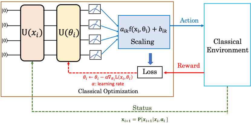
Figure 1: The flow of variational-based quantum reinforcement learning. The environment provides the input state’s features $x_{i}$ at step $i$. The features are encoded to the quantum state by parameterized circuits. Then, the quantum state evolves with the parameters layer $\mathrm{U}(\theta_{i})$ and the state is measured by projective operator repeatedly. The classical computer calculates the loss function by the scaled circuit output based on the measurements. The agent chooses an action $a_{i}$ through the policy, which is dependent on the circuit output, and the agent executes the action on the environment. It receives the reward and next state’s features $x_{i+1}$ from the environment. The classical computer calculates the new loss function dependent on the rewards and policy. The trainable parameters $\theta_{i},a_{ik},\text{and }b_{ik}$ are updated to minimize the loss function.

II Preliminary

Here we briefly recap classical reinforcement learning (RL) in Section II.1, RL with variational quantum circuit (VQC) in Section II.2 and introduction to the OpenAI Gym in Section II.3.

II.1 Classical reinforcement learning

Markov decision process (MDP) Sutton and Barto (1998) provides a dynamical framework that captures two key features in classical reinforcement learning (RL); namely, trial and error as well as delayed rewards Sutton and Barto (2018). An MDP can be described as a 5-tuple, $\mathcal{M}=(\mathcal{S},\mathcal{A},\mathcal{P},\mathcal{R},\gamma)$, where $\mathcal{S}\in\mathbb{R}^{d}$ is the state space, $d$ is the dimension of states, $\mathcal{A}\in\mathbb{R}$ is the action space, $\mathrm{P}(x_{i+1}|x_{i},a_{i})\in\mathcal{P}$ is the probability of transitioning into state $x_{i+1}$ upon taking action $a_{i}$ in state $x_{i}$, $(x_{i},a_{i})\in\left(\mathbb{R}^{d},\mathbb{R}\right)$ is the state-action pairs at step $i$, $\mathcal{R}\in{[0,R_{\text{max}}]}$ is the reward space, $R_{\text{max}}\in\mathbb{N}$ is a constant, and $\gamma\in\left[0,1\right)$ is the discount factor Bellman (1957). An agent begins at an initial state $x_{0}$ sampled from an initial distribution $\mathrm{P}(x_{0})$. Then it implements the policy $\mathrm{\pi}(a_{i}|x_{i})\in[0,1]$ to take action $a_{i}\in\mathcal{A}$ at step $i$ from a state $x_{i}\in\mathcal{S}$ and moves to a next state $x_{i+1}\sim\mathrm{P}(\cdot|x_{i},a_{i})$. The next state $x_{i+1}$ is dependent on the current state $x_{i}$ and the agent’s action $a_{i}$. After each action, the agent receives a reward $\mathrm{r}_{i}=\mathrm{R}(x_{i},a_{i})\in\mathcal{R}$. Therefore, the relation between action and reward is similar to trial and error, and the reward function $\mathrm{r}_{i}$ is associated with delayed rewards.

The goal of modern RL with classical neural network (NN) is to maximize the discount expected rewards

$$\mathrm{R}_{i}(\tau)=\hat{\mathbb{E}}_{\pi}\left[\sum_{i=0}^{T}\gamma^{i}\operatorname{r}_{i}(x_{i},a_{i})\right],$$ (1)

where $\tau=(x_{0},a_{0},x_{1},a_{1},\dots,x_{i},a_{i})$ is the trajectory in an episode, $\hat{\mathbb{E}}_{\pi}\left[\dots\right]$ denotes the expectation value under all possible policies. For the agent with the state $x_{i}$ at time $i$, the probability of the agent to take the action $a_{i}$ is $\mathrm{\pi}_{\theta_{i}}(a_{i}|x_{i})$. The agent learns the stochastic policy $\mathrm{\pi}_{\theta_{i}}(a_{i}|x_{i})$ that is dependent on $x_{i}$ and $\theta$, where $\theta_{i}\in\mathbb{R}^{m}$ is trainable parameters in classical NN, $m\in\mathbb{N}$ is the dimension of parameters to reach high expected reward. The policy is improved through updating the parameters by gradient ascent $\theta_{i}\leftarrow\theta_{i}+\eta\nabla\operatorname{L}(x_{i},{\theta_{i})}$, where $\operatorname{L}(x_{i},{\theta_{i})\in\mathbb{R}}$ is the loss function, $\eta\in\mathbb{R}$ is learning rate.

Defining the loss function plays a crucial part in optimization problems. The loss function of the PPO-clip is as follows:

$$\operatorname{L}(x_{i},\theta_{i})$$ (2)

$$= \hat{\mathbb{E}}_{\pi}\left[\min\left(\operatorname{r}_{i}(\theta_{i})\operatorname{\hat{A}}_{i},\operatorname{clip}\left(\operatorname{r}_{i}(\theta_{i}),1-\epsilon,1+\epsilon\right)\operatorname{\hat{A}}_{i}\right)\right],$$

where $\operatorname{r}_{i}(\theta_{i})=\frac{\operatorname{\pi}_{\theta_{i}}(a_{i}|x_{i})}{\operatorname{\pi}_{\theta^{\prime}_{i}}(a_{i}|x_{i})}$ is the ratio of new and old policy, ${\theta^{\prime}_{i}}$ is the policy parameters before the update, $\epsilon\in\mathbb{R}$ is usually a small number. PPO-clip is an robust algorithm in various experimental tests Schulman et al. (2017). Moreover, it is commonly used in RL algorithms for the OpenAI Gym because it is easily operated with good performance.

II.2 Reinforcement learning using variational quantum circuit

The VQC-based QRL is illustrated in Fig. 1. The key concept of VQC-based QRL Chen et al. (2020d); Lockwood and Si (2020); Jerbi et al. (2021); Skolik et al. (2021); Lan (2021); Chen et al. (2021c); Kwak et al. (2021a) is to learn the policy to acquire the maximum expected rewards $\mathrm{R}_{i}(\tau)=\hat{\mathbb{E}}_{\pi}\left[\sum_{t=0}^{T}\gamma^{i}\operatorname{r}_{i}(x_{i},a_{i})\right]$ by replacing the classical NN with VQC.

First, the input data features $x_{i}$ at step $i$ from the environment are transferred as $|\Psi_{\text{in }}(x_{i})\rangle=\operatorname{U}(x_{i})|0\rangle$, where $|0\rangle\in\mathbb{C}^{2^{n}}$ is the initial state, $n\in\mathbb{N}$ is the number of qubit, $|\Psi_{\text{in}}(x_{i})\rangle\in\mathbb{C}^{2^{n}}$ is the quantum state after encoding the input $x_{i}$, and the operator $\operatorname{U}(x_{i})$ is an unitary dependent on $x_{i}$. Then, the quantum state $|\Psi_{\text{in}}(x_{i})\rangle$ evolves by the operator $\operatorname{U}(\theta_{i})$, where $\operatorname{U}(\theta_{i})$ is an unitary, $\theta_{i}\in\mathbb{R}^{m}$ is the trainable parameters in VQC, $m\in\mathbb{N}$ is the dimension of parameters. The resultant quantum state is measured by projective operator. A general form of circuit output is

$$\mathrm{f}(x_{i},{\theta}_{i})=\left\langle 0^{\otimes n}\left|\operatorname{U}^{\dagger}(x_{i},\theta_{i})\operatorname{M}\operatorname{U}(x_{i},\theta_{i})\right|0^{\otimes n}\right\rangle,$$ (3)

where $\operatorname{U}(x_{i},\theta_{i})\in\mathbb{M}_{2^{n}}$ is an unitary operator that depends on the input and trainable parameters, and $\operatorname{M}\in\mathbb{M}_{2^{n}}$ is a projective operator.

Second, the circuit output based on the measurement is scaled linearly by parameters, $\mathrm{y}_{ip}^{\prime}=a_{ip}\times\mathrm{f}(x_{i},\theta_{i})+b_{ip}$, where $a_{ip},b_{ip}\in\mathbb{R}$ are the trainable parameters at step $i$, where $p$ is the index of actions.

The agent’s policy decides the probability of action $a$ depending on the scaled output

$$\mathrm{P}_{\theta_{i}}(a_{i}|x_{i})=\pi_{\theta_{i}}(a_{i}|x_{i})=\operatorname{Softmax}\left(\mathrm{y}_{ip}^{\prime}\right)=\frac{\mathrm{e}^{\mathrm{y}_{ip}^{\prime}}}{\sum_{p=1}^{k}\mathrm{e}^{\mathrm{y}_{ip}^{\prime}}},$$ (4)

where $a_{i}$ is the action at the state $x_{i}$, and $k$ is the number of actions. After interacting with the environment, the agent receives the reward and next state $x_{i+1}$. The loss functions $\operatorname{L}(x_{i},\theta_{i})\in\mathbb{R}$ are dependent on the scaled output and the cumulative rewards. Finally, all trainable parameters, namely $\theta_{i},a_{ip},\text{and }b_{ip}$ are optimized by gradient descent on a classical optimizer.

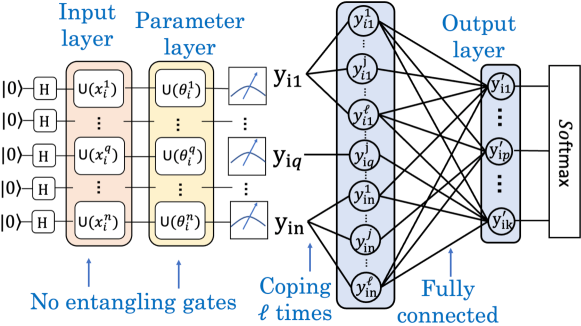
Figure 2: The architecture composes of three parts: input, parameter, and output layers. For input layer, the environment provides $n$-dimensional state with $x_{i}^{q}$ being the input state of qubit $q$, and for the CartPole, Acrobot, and LunarLander environments, the dimension of the input state also corresponding to the number of qubits are $n$ = 4, 6, and 8, respectively. The input state $x_{i}^{q}$ is encoded by the angle of a single-qubit rotational gate $\mathrm{U}(x_{i}^{q})$. In the parameters layer, we use the trainable parameters $\theta_{i}^{q}$ to control single-qubit gates and the circuit has no entangling gates. In the output layer, the output of each qubit in the circuit is reused (copied) $\ell$ times and then all outputs are connected with classical NN. $\mathrm{y}^{j}_{iq}$ is the $j\text{th}$ copy of the output of the $q\text{th}$ qubit at step $i$, $\mathrm{y}_{iq}$. The duplicated outputs $\mathrm{y}^{j}_{iq}$ with $q=1,\dots,n$ and $j=1,\dots,\ell$ are fed into the classical fully-connected NN to produce the scaled circuit outputs $\mathrm{y}_{ip}^{\prime}$ with $p=1,\dots,k$. Finally, we add the Softmax function to transfer the scaled circuit outputs to probability distribution.

Table 2: The performance metrics for several OpenAI Gym environments.

Environment	Number of status	Number of actions	The metric of performance
CartPole-v0	4	2	Average reward of 195.0 over 100 consecutive trials.
CartPole-v1	4	2	Average reward of 475.0 over 100 consecutive trials.
Acrobot-v1	6	3	Do not define ”solving” condition. Look at the $\href https://github.com/openai/gym/wiki/Leaderboard$ to evaluate the model.
LunarLander-v2	8	4	Average reward of 200 over 100 consecutive trials.

II.3 OpenAI Gym environments

OpenAI Gym provides benchmarking environments for RL tasks to compare their model performance. CartPole, Acrobot, and LunarLander tasks are regarded as the basic environments in OpenAI Gym. The schematic diagrams and the performance metrics which measure how well RL agents can achieve the intended goals of these three tasks are shown in Fig. 4 (a)-(c) and Table 2, respectively.

The goal of the CartPole task is to balance the pole on a cart by moving the cart. A reward of $+1$ is given for each step that the pole remains upright. The episode ends when the pole is more than 12 degrees from vertical, or the cart moves more than 2.4 units from the center.

Acrobot-v1 is another classical control task in the Gym. The system includes two joints and two links, where the joint between the two links is actuated. Initially, the links are hanging downwards, and the goal is to swing the end of the lower link up to a given height.

LunarLander is a more complex task than CartPole and Acrobot tasks. Its goal is to let the agent learn to land between the two yellow flags. The agent controls up to four actions corresponding to no action, the main engine is firing down, and the engine is firing left or right.

More descriptions about the CartPole, Acrobot and LunarLander environments together with discussions on input data encoding schemes, measurements and VQC-based quantum RL can be found in Appendix A.

III A novel variational quantum reinforcement learning with single-qubit

To improve the performance based on the VQC method in OpenAI Gym tasks, we propose a new architecture, SVQC, which is composed of three parts: input, parameter, and output layers shown in Fig. 2. For input layer, the environment provides an input state $x_{i}$ to the input layer. The state $x_{i}$ is encoded by the angle of a single-qubit rotational gate $\mathrm{U}(x_{i})$. The number of the data encoding rotational gates is usually determined by the state dimension.

In the parameters layer, trainable parameters $\theta_{i}$ control the single-qubit rotational gates $\mathrm{U(\theta_{i})}$ and are updated through gradient descent. Here, we only use the single-qubit gates without entangling gates to overcome the problem of the barren plateau caused by entangling gates in the optimization process Ortiz Marrero et al. (2021).

The output layer is decomposed by three components: measurements, connection with a classical NN, and output reuse strategies. First, the expectation value of the measurements is obtained from Eq. (3) denoted by

$$\mathrm{y}_{iq}=\mathrm{f}(x_{i}^{q},\theta_{i}^{q})=\left\langle 0\left|\operatorname{U}^{\dagger}(x_{i}^{q},\theta_{i}^{q})\operatorname{Z}_{q}\operatorname{U}(x_{i}^{q},\theta_{i}^{q})\right|0\right\rangle,$$ (5)

where $q=1,\dots,n$ is the indexes for different single qubits in the quantum circuit, $\operatorname{Z}_{q}$ is the Pauli Z matrix of qubit $q$, and $\operatorname{U}(x_{i}^{q},\theta_{i}^{q})\in\mathbb{C}^{2\times 2}$ is a single-qubit unitary operator. Since the SVQC outputs merely come from the expectation values of eigenvalues on the unitary family $\{\operatorname{U}^{\dagger}(x_{i}^{q},\theta_{i}^{q})\operatorname{Z}_{q}\operatorname{U}(x_{i}^{q},\theta_{i}^{q})\}$, the following technical strategies can enrich the expressive power of its outputs. Second, we link the single-qubit-based quantum circuit with a fully-connected NN layer to increase the expressive power of the quantum circuit so that it is more likely to achieve the optimal result in the practical optimization process Jerbi et al. (2021); Goto et al. (2021). Given that there exist optimal circuit outputs $\mathrm{y}_{ip}^{\prime*}(x_{i}^{q},\theta_{i}^{q})\in\mathbb{R}$ for variety tasks on OpenAI Gym, our target is to minimize $|\mathrm{y}_{ip}^{\prime}-\mathrm{y}_{ip}^{\prime*}|$, where $\mathrm{y}_{ip}^{\prime}\in\mathbb{R}$ is the scaled quantum circuit output for $p=1,\dots,k$:

$${\small\left(\begin{array}[]{c}\mathrm{y}_{i1}^{\prime}\\ \vdots\\ \mathrm{y}_{ip}^{\prime}\\ \vdots\\ \mathrm{y}_{ik}^{\prime}\end{array}\right)=\left(\begin{array}[]{c}{b}_{i1}\\ \vdots\\ {b}_{ip}\\ \vdots\\ {b}_{ik}\end{array}\right)+\left(\begin{array}[]{ccccc}W_{11}^{i}&\cdots&W_{1q}^{i}&\cdots&W_{1n}^{i}\\ \vdots&\ddots&\vdots&\ddots&\vdots\\ W_{p1}^{i}&\cdots&W_{pq}^{i}&\cdots&W_{pn}^{i}\\ \vdots&\ddots&\vdots&\ddots&\vdots\\ W_{k1}^{i}&\cdots&W_{kq}^{i}&\cdots&W_{kn}^{i}\end{array}\right)\left(\begin{array}[]{c}\mathrm{y}_{i1}\\ \vdots\\ \mathrm{y}_{iq}\\ \vdots\\ \mathrm{y}_{in}\end{array}\right)},$$ (6)

where $W_{pq}\in\mathbb{R}$ is the trainable parameters (weights) in the NN, $b_{ip}\in\mathbb{R}$ are the biases, $k$ is the number of actions and $n$ is the number of qubits. Comparing the domain of $\mathrm{y}_{iq}$ with that of $\mathrm{y}_{ip}^{\prime}$ in Eqs. (5) and (6), the latter can increase the expressive power of the circuit output according to the studies in Ref. Jerbi et al. (2021); Goto et al. (2021).

Table 3: Details of model settings for different RL environments. The quantum circuits shown in Fig. 2 are employed to complete the different RL tasks. The initial state is set to be in the ground state while the input layer is composed of a Hadamard gate followed by the gate sequence of (Ry($x^{q}_{i}$)-Rz($x^{q}_{i}$), where $q=1,\ldots,n$ are the qubit indexes. The parameterized single-qubit gate is Ry($\theta^{q}_{i}$). The number of qubits for the CartPole, Acrobot, and LunarLander environments are $n$ = 4, 6, and 8, respectively. Then the repeated measurements of $\sigma_{z}^{q}$ are performed in the output layer. Finally, the measurement outputs could be reused for certain times and then connected with a fully-connected classical NN layer. The numbers appearing in the parentheses of FCN and CNN are the numbers of nodes in the fully-connected classical NN layers.

Environment	Learning algorithm	Architecture (qubit number $n$)	Times of reuses ($\ell$)	Number of actions ($k$)
CartPole-v1	Algorithm 1	$|0\rangle$-H-Ry($x^{q}_{i}$)-Rz($x^{q}_{i}$)-Ry($\theta^{q}_{i}$), $n=4$	16	2
CartPole-v1	Classical PPO	FCN (16, 32, 64, 32, 2)	None
CartPole-v1	Classical PPO	CNN (5, 2, 4, 2)	None
Acrobot-v1	Algorithm 1	$|0\rangle$-H-Ry($x^{q}_{i}$)-Rz($x^{q}_{i}$)-Ry($\theta^{q}_{i}$), $n=6$	8	3
Acrobot-v1	Classical PPO	FCN (16, 32, 64, 32, 3)	None
Acrobot-v1	Classical PPO	CNN (5, 2, 4, 2, 3)	None
LunarLander-v2	Algorithm 1,  2	$|0\rangle$-H-Ry($x^{q}_{i}$)-Rz($x^{q}_{i}$)-Ry($\theta^{q}_{i}$), $n=8$ repeated 3 times	8	4
LunarLander-v2	Classical PPO	FCN (16, 32, 64, 32, 4)	None

Algorithm 1 Hybrid Quantum PPO (QPPO) algorithm

Input: State: $(x_{1},s_{2},\dots,x_{i})$
      Output: Action: $a_{i}$

for episode do

     Transfer from classical state $x_{i}$ to quantum stat $|\psi\left(x_{i}\right)\rangle$

     Actor collect data $\operatorname{D}(s,a,r,\mathrm{P_{a}})$ through VQC

     actor’s policy $\pi_{\theta_{a}}\left(s\right)$ from environment.

     Actor VQC output $\mathrm{P_{a}}$ and action $a$.

     Memorize the $\left(s,a,r,\mathrm{P_{a}}\right)$ into experience buffer

     Critic VQC output the value$\mathrm{V}\left(s\right)$ through state $s$

     Compute discount reward $R_{t}=\sum_{t=1}^{T}\gamma^{t+T-1}\mathrm{r}$

     Compute advantage estimate $a_{i}=R_{t}-V\left(x_{i}\right)$

     if step % update-time == 0 or done then

         for epoch do

              Update critic parameters $\theta_{c}$ through minimum

              value loss $L_{v}=\frac{1}{\left|D\right|}\sum_{t=1}^{T}\left(V\left(x_{i}\right)-R_{t}\right)^{2}$

              by gradient descent with Adam.

              Update actor parameters $\theta_{a}$ through maximum

              actor loss.

              $\mathrm{L}_{a}=\frac{1}{\left|D\right|}log\sum_{t=1}^{T}{\min(\frac{\pi_{\theta}(a_{i}|x_{i})}{\pi_{\theta_{old}}(a_{i}|x_{i})}}$,

              $clip\left(1+\epsilon,1-\epsilon\right))\mathrm{A}_{t}$

              use gradient ascent with Adam.

              Update VQC actor and classical NN parameters

              $\theta_{a}\longleftarrow\ \theta_{a}+\nabla_{\theta_{a}}\mathrm{L}_{a}$.

              Clean Experience

         end for

     end if

end for

Algorithm 2 Hybrid policy on LunarLander-v2 environment.

1:if episode reward $>=$ 200 then

2:     Stop update parameters

3:     count $+=$ 1

4:     if count $>$ Max conut then

5:         Max conut $=$ count

6:         Save actor and critic policy

7:     end if

8:     if average episode reward $<$ 200 then

9:         Update actor and critic parameters

10:         count $=$ 0

11:     end if

12:end if

Finally, we duplicate the expectation value of the measurement $\ell$ times and then all outputs are fed into the classical fully-connected NN layer shown in Fig. 2. The final scaled output with the duplicated qubit outputs reads

$$\mathrm{y}_{ip}^{\prime}={b}_{ip}+{W}_{p1}^{i\#}\mathrm{y}_{i1}^{\prime}+\dots+{W}_{pq}^{i\#}\mathrm{y}_{iq}^{\prime}+\dots+{W}_{pn}^{i\#}\mathrm{y}_{in}^{\prime},$$ (7)

where $W_{kj}^{i\#}=W^{i(1)}_{kj}+W^{i(2)}_{kj}+\cdots+W^{i(\ell)}_{kj}$ is the expected weights with duplicated outputs, $n\in\mathbb{N}$ denotes the $n\text{th}$ qubit, and $\ell\in\mathbb{N}$ is the number of the output reuse. It will be shown later that the method of reusing qubit outputs improves the sample efficiency.

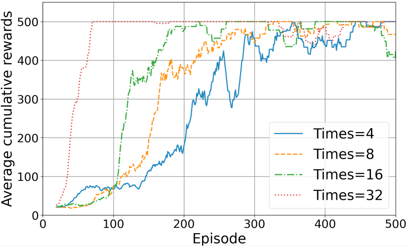
Figure 3: Performances of the quantum RL agents for different numbers of output reuse of 4, 8, 16 and 32 times for the CartPole environment. The x-axis is the number of episodes, and the y-axis is the average cumulative reward, averaged over the last 20 episodes.

Table 4: Hyperparameters of different models

Environment	Learning algorithm	Architecture	Actor Learning rate	Critic Learning rate	Discount factor	epoch	Clip $\epsilon$
CartPole-v1	VQC-PPO Alg. 1	Fig. 2	0.001	0.01	0.99	4	0.1
CartPole-v1	VQC-PPO Alg. 1	Fig. 5(a)	0.004	0.04	0.99	4	0.1
CartPole-v1	Classical PPO	Neural network	0.0003	0.001	0.98	4	0.1
Acrobot-v1	VQC PPO Alg. 1	Fig. 2	0.004	0.04	0.98	4	0.1
Acrobat-v1	Classical PPO	Neural network	0.0003	0.001	0.98	4	0.1
LunarLander-v2	VQC PPO Alg. 1 2	Fig. 2	0.002	0.02	0.98	4	0.1

IV Numerical results and discussion

To improve sample inefficiency in OpenAI Gym tasks, we compare the learning curves of SVQC, MVQC, and classical NNs on different tasks. Moreover, we use the IBM quantum devices to test the CartPole, Acrobot, and LunarLander tasks for comparing the real devices with an ideal simulator. In the following, the detailed discussion of simulator results are shown in Section IV.1 and the results of IBM quantum devices are shown in Section IV.2. The details of model settings including circuit architectures and learning algorithms of SVQC, classical fully-connected neural network (FCN), and convolution neural network (CNN) for simulations of different RL environments on simulators are described in Table 3. The detailed hyperparameters of the simulation models are shown in Table 4.

IV.1 Results on simulator

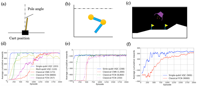
Figure 4: Illustrations and Performances of the single-qubit VQC PPO using single-qubit systems with output reuse strategy, classical fully-connected neural network (FCN) and convolutional neural network (CNN) in the RL optimization process for (a)(d) CartPole, (b)(e) Acrobot, and (c)(f) LunarLander problems. The numbers in the parentheses of different models are the total trainable parameters used in these models, respectively. The x-axis is the number of episodes and the y-axis represents the average cumulative reward, averaged over the last 20 episodes, at that episode. The CartPole and Acrobot experimental results are averaged over five runs and the LunarLander result is the best one in 10 runs. The sample efficiency follows approximately the relationship of SVQC $>$ classical FCN $\approx$ CNN $>$ Multi-qubit VQC.

Table 5: Relaxation time $T_{1}$, dephasing time $T_{2}$, single-qubit $\sqrt{\mathrm{X}}$, X, and identity (ID) gate errors and readout error data of different quantum machines downloaded from IBM Quantum service at the time when the experiments were performed.

Machine	$\mathrm{T}_{1}$ (us)	$\mathrm{T}_{2}$ (us)	Readout assignment error	Readout length (ns)	ID error	$\sqrt{\mathrm{X}}(\mathrm{S_{x}})$ error	Single-qubit Pauli-X error
ibmq_lagos	75.65	39.3	1.16E-02	704	3.11E-04	3.11E-04	3.11E-04
Ibmq_belem	86.5	100.93	2.46E-02	5351.111	2.33E-04	2.33E-04	2.33E-04
Ibmq_lima	87.9	87.83	2.49E-02	5351.111	5.31E-04	5.31E-04	5.31E-04
ibmq_jakarta	91.96	41.46	3.41E-02	5351.111	3.84E-04	3.84E-04	3.84E-04
ibmq_toronto	92.3	55.67	4.57E-02	5201.778	2.34E-04	2.34E-04	2.34E-04

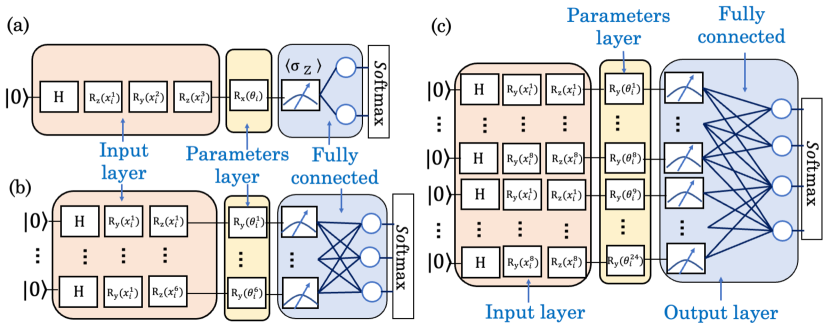
Figure 5: Architectures of the SVQC models for the (a) CartPole-v0, (b) Acrobat-v1 and (c) LunarLander-v2 task for the tests on real quantum devices and a simulator. H stands for the Hadamard gate. $x^{j}_{i}$ is the $j\mathrm{th}$ feature state on the $i\mathrm{th}$ episode. $\theta^{q}_{i}$ is the trained parameters on the $q\mathrm{th}$ qubit in the quantum circuit on the $i\mathrm{th}$ episode.

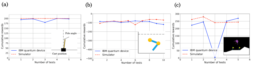
Figure 6: Performances of the tests of the SVQC RL agents for the (a) CartPole-v0, (b) Acrobat-v1 and (c) LunarLander-v2 tasks on IBM quantum devices and a simulator. The x-axis is the index number of the tests. The y-axis is the cumulative rewards in one episode. The mean rewards of CartPole, Acrobot and LunarLander on the quantum devices are 194.0, -90.04, and 198.3, and the standard deviations are 8.12, 5.03, and 19.3, respectively. The average rewards of CartPole, Acrobot and LunarLander on the ideal simulator are 200.0, -84.40, and 253.4, and the standard deviations are 0, 18.8, and 17.1, respectively.

The training processes of SVQCs in the CartPole and Acrobot tasks are attained through Algorithm 1, while both Algorithm 1 and Algorithm 2 are used in the LunarLander-v2 task. The performances for different numbers of the reused outputs for the CartPole environment is shown in Fig. 3, indicating that the method of reusing qubit outputs improves the sample efficiency. The learning curves of the various models on the tasks of CartPole, Acrobot, and LunarLander are shown in Fig. 4 (d)-(f), respectively.

For the CartPole task, we compare the sample efficiency of single-qubit VQC (SVQC), multi-qubit VQC (MVQC), classical FCN, and CNN in Fig. 4 (d). Our work uses the SVQC architecture shown in Fig. 2 and described in Table 3. The MVQC model for RL is discussed in some detail in $\href https://www.tensorflow.org/quantum/tutorials/quantum_reinforcement_learning$ and the circuit architecture of MVQC used here is from Jerbi et al. (2021). Descriptions about the architectures of classical FCN and CNN used here can be found in Table 3. From Fig. 4 (d), we find that SVQC (thick solid line) achieves maximum rewards in about 150 episodes. In comparison, MVQC (dashed line) converges around 500 episodes without achieving the maximum rewards while FCN (8,800) (dash-dot line), FCN (357) (dotted line), and CNN (173) reach the maximum rewards in about 400, 1,600, and 1650 episodes, respectively. Note that the numbers in the parentheses of different models are the total trainable parameters used in these models, respectively. These results provide concrete numerical evidence that SVQC could improve sample efficiency by about three times compared to classical FCN (8,800) under the same optimization process.

For the Acrobot task, we compare the sample efficiency of SVQC, classical fully-connected neural network (FCN), and convolution neural network (CNN) in Fig. 4 (e). From the figure, we find SVQC (solid line) achieves the average rewards of -90 in around 90 episodes while FCN (8,800) (dashed line), FCN (250) (dash-dot), and CNN (1,000) (dash-dot) reach the average reward of -90 in about 250, 600, and 1000 episodes. These results also indicate that SVQC could improve the sample efficiency by about three times compared to classical FCN (8,800) under the same optimization process.

For the Luarlander task, we compare the sample efficiency of SVQC and FCN in Fig. 4 (f). The figure shows that SVQC (solid line) achieves the average rewards of about 220 in 1,000 episodes. In comparison, FCN (dashed line) reaches the average rewards of 200, slightly lower than SVQC, in 1,750 episodes. These results conclude that the SVQC improves the sample efficiency by about two times compared to classical FCN (9,000) under the same optimization process. We would like to emphasize that this is the first time that the more complex control task of LunarLander can be achieved in the quantum RL field.

In conclusion, our proposed SVQC achieves higher rewards than existing VQC-based models Lockwood and Si (2020); Jerbi et al. (2021); Skolik et al. (2021); Kwak et al. (2021b) and improves the sample efficiency (speed of convergence) compared to the classical fully-connected neural networks in the CartPole and Acrobot tasks. Moreover, our SVQC uses much (at least one order of magnitude) fewer trainable parameters with even better learning performance than the best performing FCNs shown in Fig. 4 (d)-(f).

IV.2 Implementation on IBM quantum devices

In this section, we feed the trained parameters of our SVQCs into the IBM quantum devices, and compare their performance with that of the ideal simulators. The chosen benchmarking environments are CartPole-v0, Acrobot-v1, and LunarLander-v2 in OpenAI Gym. The real quantum device experiments for the CartPole and Acrobot tasks are executed on “ibm_lagos” and “ibm_belem”, while the LunarLander task is on “ibm_lima”, “ibm_jakarta” and “ibm_toronto”.

The cumulative rewards on the CartPole-v0, Acrobot-v1, and LunarLander-v2 tasks are shown in Fig. 6 (a)-(c) and the numbers of measurements for these tasks are 1024, 1024, and 8192, respectively. Details of the used hyperparameters can be found in Table. 5, and we will elaborate on the circuit architectures and their performances below.

We employ the quantum circuit in Fig. 5 (a) to conduct the task of CartPole-v0, where only a single qubit initialized in the ground state, $|0\rangle$, is required. The input layer consists of a Hadamard gate and the sequence of (Rz, Ry, Rz) gates; while the parameter layer contains only an Rx gate. We import four classical trained parameters to scale the circuit output and use a trainable parameter for the angle of Rx. We upload the trained model parameters of the SVQC model in Fig. 5 (a) to IBM Quantum devices. According to Fig. 6(a), we find that the average reward of the real device over five tests is 190. This reward is comparable with the average reward, 200, obtained on the ideal simulator.

The six-qubit quantum circuit shown in Fig. 5 (b) is used to complete the Acrobot-v1 task. Similarly, the initial state is set to be in the ground state while the input and parameter layers are composed of a Hadamard gate followed by the gate sequence of (Ry, Rz, Ry). Then the repeated measurements of $\sigma_{z}$ are performed in the output layer. This circuit consists of six trainable rotational angles and 21 parameters for output rescaling. The average reward obtained from the quantum machine is -90 while the value from the ideal simulator is -84. Again, the rewards of the real device and the idea simulator are comparable.

The first quantum RL agent based on SVQC consisting of a 24-qubit quantum circuit with the architecture demonstrated in Fig. 5 (c) is used to complete the LunarLander-v2 task on the real quantum device. The circuit inherits the architecture of SVQC used in the Acrobot-v1 task and is further expanded to a larger scale by introducing 24 trainable angle parameters and 100 output scaling parameters. By comparing the average reward of the real device with that of the ideal simulator in Fig. 6 (c), we find the average reward of the real device is 200, slightly worse than the average reward of 250 of the ideal simulator. We expect that conducting more test runs will further increase the average reward of the real device, but we did not continue the experiments on IBM devices due to the cost of the expensive quantum computational resources.

To the best of our knowledge, it is the first time the complex RL tasks can be accomplished on IBM quantum devices. The results demonstrate that even though the training is on the quantum simulator without noise, the trained SVQC models have similar performances on current NISQ devices compared to the ideal simulator.

V Conclusion and future work

The SVQC performs better than previous studies Lockwood and Si (2020); Jerbi et al. (2021); Skolik et al. (2021); Kwak et al. (2021b) which use several CNOT or CZ gates on the CartPole and Acrobot environments. This leads to an open question of “What are the roles of entangling gates in MVQC for the RL tasks?” On the other hand, we find SVQC with the output reuse can solve the RL tasks more efficiently than the classical NNs. This brings the question of “What is the quantum-inspired algorithm, which can solve the RL problems efficiently?” Since SVQC can be implemented on the current NISQ quantum devices to handle classical control and box2d tasks in openAI Gym. Therefore, “What is the limitation on the current NISQ devices in RL tasks?” is the remaining question for the future work.

VI Acknowledgments

J.Y.H and H.S.G. thank IBM Quantum Hub at NTU for providing computational resources and accesses for conducting the real quantum machine experiments. H.S.G. acknowledges support from the the Ministry of Science and Technology of Taiwan under Grants No. MOST 109-2112-M-002-023-MY3, No. MOST 109-2627-M-002-003, No. MOST 110-2627-M-002-002, No. MOST 107-2627-E-002-001-MY3, No. MOST 111-2119-M-002-006-MY3 and No. MOST 110-2622-8-002-014 from the US Air Force Office of Scientific Research under award number FA2386-20-1-4033, and from the National Taiwan University under Grant No. NTU-CC-111L894604.

Code availability: The Codes that support the findings of this study and all trained parameters in different tasks are available at $\href https://github.com/Yueh-H/single-qubit-RL$.

Appendix A Supplementary materials of variational quantum circuits and the environments

In this Appendix, we discuss the variational quantum circuit (VQC) in Sec. A.1, the architecture of VQC-based quantum reinforcement learning in Sec. A.2, and the detailed constraints on different environments on OpenAI Gym in Sec. A.3.

A.1 Discussion of variational quantum circuits

When it comes to quantum computation, the goal is to find the quantum advantage. The potential advantage in VQC is to use the vast Hilbert space in the quantum information process Schuld and Killoran (2019); Biamonte et al. (2017). There are several steps of VQC to explore the potential of the advantage. Let the data set $\mathcal{D}={\{x_{1},\dots,x_{M}\}}$ has $M$ feature data and each is an $N$-dimensional real feature vector.

1. State preprocess layer:

   There are three main encoding strategies of the quantum circuit: basis, amplitude Farhi and Neven (2018); Schuld et al. (2020), and Hamiltonian encoding schemes. The basis encoding scheme needs the runtime of $\mathcal{O}(MN)$ for state preparation without QRAM Giovannetti et al. (2008), while the amplitude and Hamiltonian encoding schemes can reduce the time to $\mathcal{O}(\log(MN))$ with QRAM. Moreover, the Hamiltonian encoding tries to build the kernel space, which is hard to be built using classical computers Havlíček et al. (2019b).

2. Parameter layer:

   There are different technologies to design the different architectures of the circuit by machine learning Du et al. (2020c) or reinforcement learning Kuo et al. (2021); Ye and Chen (2021).

3. Measurement:

   The general quantum circuit output is $\left\langle\sigma_{z}\right\rangle=\operatorname{tr}\left(\operatorname{\rho}(x_{i},\theta_{i})\operatorname{\sigma_{z}}\right)$, where $\rho(x_{i},\theta_{i})\in\mathbb{C}^{2^{n}\times 2^{n}}$ is the density matrix depending on parameters and input data, and $\sigma_{z}\in\mathbb{C}^{2^{n}\times 2^{n}}$ is the projective matrix. A challenge about the measurement is that lots of shots would eliminate the runtime advantage Ciliberto et al. (2018); Aaronson (2015). There are strategies to improve the efficiency in measuring the quantum state Du et al. (2021c); Zhang et al. (2021).

4. Optimization:

   The challenge about circuit optimization lies in barren plateau McClean et al. (2018). The gradient of parameters would vanish exponentially in the optimization process. Using tree structure Zhang et al. (2020b), tuning the parameters with an iterative optimization structure, and using adaptively selected Hamiltonian Liao et al. (2021) can mitigate the barren plateau in the process.

A.2 Discussion of VQC-based quantum reinforcement learning

There are many technical skills in VQC-based quantum reinforcement learning. References Jerbi et al. (2021); Skolik et al. (2021); Lan (2021) provide various methods to solve the OpenAI Gym tasks. The methods can be divided by the circuit architecture that consists of the input, parametric, and output layers.

In the input layer, the additional trainable parameters are encoded by the rotational angles of the gates that improve the performance on the Cartpole and Acrobot tasks Jerbi et al. (2021); Skolik et al. (2021). For the input and parametric layers, the repeated application of re-uploading enhances the performance on the classical control tasks Jerbi et al. (2021); Skolik et al. (2021); Lan (2021). In the output layer, introducing the extra trainable parameters to rescale the measurement outcomes Jerbi et al. (2021); Skolik et al. (2021) or adding the classical neuron network connection improves the cumulative rewards Lan (2021) on the Cartpole and Pendulum tasks.

Table 6: Constrains on the observations of the Cartpole environment. The termination condition is that the pole exceeds 12 degrees or the Cart position exceeds 2.4 or -2.4.

Observation	Min	Max
Cart Position $x$	-4.8	4.8
Cart Velocity $v$	$-\mathrm{Inf}(-\infty)$	$\mathrm{Inf}\ (+\infty)$
Pole Angle $\theta$	-0.418 rad	0.418 rad
Pole Angular Velocity $\theta$	$-\mathrm{Inf}\ (-\infty)$	$\mathrm{Inf}\ (+\infty)$

Table 7: Constrains on the observations of the Acrobot environment. The episode terminates when the end of the lower link exceeds the given height or the agent does not achieve the condition within 500 time steps.

Observation	Min	Max
upper pole cos	-1	1
upper pole sin	-1	1
down pole cos	-1	1
down pole sin	-1	1
Upper angular velocity	-4$\pi$	4$\pi$
down angular velocity	-9$\pi$	9$\pi$

A.3 Introduction to the OpenAI Gym environment

The followings are the constraints on the Cartpole, Acrobot, and LunarLander environments. The number of states of Cartpole , Acrobot, and LunarLander are four, six, and eight, respectively, and the numbers of actions are two, three, and four, respectively. The constrains on different observations (states) of Cartpole and Acrobot are subsequently shown in Table. 6 and Table. 7.

The detailed information of LunarLander is as follows. According to the description of the environment in OpenAI Gym, the reward for moving from the top of the screen to the landing pad and zero speed falls between 100 and 140 points. The episode finishes if the lander crashes or comes to rest, receiving an additional reward of $-100$ or $+100$ points. Each leg ground contact is $+10$. The reward is −0.03 for firing the side engine, and −0.3 for firing the main engine each frame.

References

- Sutton and Barto (2018) R. S. Sutton and A. G. Barto, Reinforcement Learning: An Introduction (A Bradford Book, Cambridge, MA, USA, 2018).
- Silver et al. (2017) D. Silver, T. Hubert, J. Schrittwieser, I. Antonoglou, M. Lai, A. Guez, M. Lanctot, L. Sifre, D. Kumaran, T. Graepel, T. Lillicrap, K. Simonyan, and D. Hassabis, Mastering chess and shogi by self-play with a general reinforcement learning algorithm (2017), arXiv:1712.01815 [cs.AI] .
- Vinyals et al. (2019) O. Vinyals, I. Babuschkin, W. M. Czarnecki, M. Mathieu, A. Dudzik, J. Chung, D. H. Choi, R. Powell, T. Ewalds, P. Georgiev, J. Oh, D. Horgan, M. Kroiss, I. Danihelka, A. Huang, L. Sifre, T. Cai, J. P. Agapiou, M. Jaderberg, A. S. Vezhnevets, R. Leblond, T. Pohlen, V. Dalibard, D. Budden, Y. Sulsky, J. Molloy, T. L. Paine, C. Gulcehre, Z. Wang, T. Pfaff, Y. Wu, R. Ring, D. Yogatama, D. Wünsch, K. McKinney, O. Smith, T. Schaul, T. Lillicrap, K. Kavukcuoglu, D. Hassabis, C. Apps, and D. Silver, Nature 575, 350 (2019).
- Wurman et al. (2022) P. R. Wurman, S. Barrett, K. Kawamoto, J. MacGlashan, K. Subramanian, T. J. Walsh, R. Capobianco, A. Devlic, F. Eckert, F. Fuchs, L. Gilpin, P. Khandelwal, V. Kompella, H. Lin, P. MacAlpine, D. Oller, T. Seno, C. Sherstan, M. D. Thomure, H. Aghabozorgi, L. Barrett, R. Douglas, D. Whitehead, P. Dürr, P. Stone, M. Spranger, and H. Kitano, Nature 602, 223 (2022).
- Degrave et al. (2022) J. Degrave, F. Felici, J. Buchli, M. Neunert, B. Tracey, F. Carpanese, T. Ewalds, R. Hafner, A. Abdolmaleki, D. de las Casas, C. Donner, L. Fritz, C. Galperti, A. Huber, J. Keeling, M. Tsimpoukelli, J. Kay, A. Merle, J.-M. Moret, S. Noury, F. Pesamosca, D. Pfau, O. Sauter, C. Sommariva, S. Coda, B. Duval, A. Fasoli, P. Kohli, K. Kavukcuoglu, D. Hassabis, and M. Riedmiller, Nature 602, 414 (2022).
- Panou and Reczko (2020) D. N. Panou and M. Reczko, Deepfoldit – a deep reinforcement learning neural network folding proteins (2020), arXiv:2011.03442 [q-bio.BM] .
- Mirhoseini et al. (2020) A. Mirhoseini, A. Goldie, M. Yazgan, J. Jiang, E. Songhori, S. Wang, Y.-J. Lee, E. Johnson, O. Pathak, S. Bae, A. Nazi, J. Pak, A. Tong, K. Srinivasa, W. Hang, E. Tuncer, A. Babu, Q. V. Le, J. Laudon, R. Ho, R. Carpenter, and J. Dean, Chip placement with deep reinforcement learning (2020), arXiv:2004.10746 [cs.LG] .
- Irpan (2018) A. Irpan, Deep reinforcement learning doesn’t work yet, https://www.alexirpan.com/2018/02/14/rl-hard.html (2018).
- Du et al. (2020a) S. S. Du, J. D. Lee, G. Mahajan, and R. Wang, Agnostic q-learning with function approximation in deterministic systems: Tight bounds on approximation error and sample complexity (2020a), arXiv:2002.07125 [cs.LG] .
- Nachum et al. (2018) O. Nachum, S. Gu, H. Lee, and S. Levine, Data-efficient hierarchical reinforcement learning (2018), arXiv:1805.08296 [cs.LG] .
- Ye et al. (2021) W. Ye, S. Liu, T. Kurutach, P. Abbeel, and Y. Gao, Mastering atari games with limited data (2021), arXiv:2111.00210 [cs.LG] .
- Whitney et al. (2021) W. F. Whitney, M. Bloesch, J. T. Springenberg, A. Abdolmaleki, K. Cho, and M. Riedmiller, Decoupled exploration and exploitation policies for sample-efficient reinforcement learning (2021), arXiv:2101.09458 [cs.LG] .
- Badia et al. (2020) A. P. Badia, P. Sprechmann, A. Vitvitskyi, D. Guo, B. Piot, S. Kapturowski, O. Tieleman, M. Arjovsky, A. Pritzel, A. Bolt, and C. Blundell, Never give up: Learning directed exploration strategies (2020), arXiv:2002.06038 [cs.LG] .
- Liu et al. (2020) G. Liu, R. Wu, H.-T. Cheng, J. Wang, J. Ooi, L. Li, A. Li, W. L. S. Li, C. Boutilier, and E. Chi, Data efficient training for reinforcement learning with adaptive behavior policy sharing (2020), arXiv:2002.05229 [cs.LG] .
- Zhang et al. (2020a) J. Zhang, J. Kim, B. O’Donoghue, and S. Boyd, Sample efficient reinforcement learning with reinforce (2020a), arXiv:2010.11364 [cs.LG] .
- Agarwal et al. (2020) A. Agarwal, S. M. Kakade, J. D. Lee, and G. Mahajan, On the theory of policy gradient methods: Optimality, approximation, and distribution shift (2020), arXiv:1908.00261 [cs.LG] .
- Bhandari and Russo (2020) J. Bhandari and D. Russo, Global optimality guarantees for policy gradient methods (2020), arXiv:1906.01786 [cs.LG] .
- Mnih et al. (2015) V. Mnih, K. Kavukcuoglu, D. Silver, A. A. Rusu, J. Veness, M. G. Bellemare, A. Graves, M. Riedmiller, A. K. Fidjeland, G. Ostrovski, S. Petersen, C. Beattie, A. Sadik, I. Antonoglou, H. King, D. Kumaran, D. Wierstra, S. Legg, and D. Hassabis, Nature 518, 529 (2015).
- Hessel et al. (2017) M. Hessel, J. Modayil, H. van Hasselt, T. Schaul, G. Ostrovski, W. Dabney, D. Horgan, B. Piot, M. Azar, and D. Silver, Rainbow: Combining improvements in deep reinforcement learning (2017), arXiv:1710.02298 [cs.AI] .
- Arute et al. (2019) F. Arute, K. Arya, R. Babbush, D. Bacon, J. C. Bardin, R. Barends, R. Biswas, S. Boixo, F. G. S. L. Brandao, D. A. Buell, B. Burkett, Y. Chen, Z. Chen, B. Chiaro, R. Collins, W. Courtney, A. Dunsworth, E. Farhi, B. Foxen, A. Fowler, C. Gidney, M. Giustina, R. Graff, K. Guerin, S. Habegger, M. P. Harrigan, M. J. Hartmann, A. Ho, M. Hoffmann, T. Huang, T. S. Humble, S. V. Isakov, E. Jeffrey, Z. Jiang, D. Kafri, K. Kechedzhi, J. Kelly, P. V. Klimov, S. Knysh, A. Korotkov, F. Kostritsa, D. Landhuis, M. Lindmark, E. Lucero, D. Lyakh, S. Mandrà, J. R. McClean, M. McEwen, A. Megrant, X. Mi, K. Michielsen, M. Mohseni, J. Mutus, O. Naaman, M. Neeley, C. Neill, M. Y. Niu, E. Ostby, A. Petukhov, J. C. Platt, C. Quintana, E. G. Rieffel, P. Roushan, N. C. Rubin, D. Sank, K. J. Satzinger, V. Smelyanskiy, K. J. Sung, M. D. Trevithick, A. Vainsencher, B. Villalonga, T. White, Z. J. Yao, P. Yeh, A. Zalcman, H. Neven, and J. M. Martinis, Nature 574, 505 (2019).
- Zhong et al. (2020) H.-S. Zhong, H. Wang, Y.-H. Deng, M.-C. Chen, L.-C. Peng, Y.-H. Luo, J. Qin, D. Wu, X. Ding, Y. Hu, P. Hu, X.-Y. Yang, W.-J. Zhang, H. Li, Y. Li, X. Jiang, L. Gan, G. Yang, L. You, Z. Wang, L. Li, N.-L. Liu, C.-Y. Lu, and J.-W. Pan, Science 370, 1460–1463 (2020).
- Wu et al. (2021) Y. Wu, W.-S. Bao, S. Cao, F. Chen, M.-C. Chen, X. Chen, T.-H. Chung, H. Deng, Y. Du, D. Fan, M. Gong, C. Guo, C. Guo, and et al., Physical Review Letters 127, 10.1103/physrevlett.127.180501 (2021).
- Hamilton et al. (2017) C. S. Hamilton, R. Kruse, L. Sansoni, S. Barkhofen, C. Silberhorn, and I. Jex, Phys. Rev. Lett. 119, 170501 (2017).
- Preskill (2018) J. Preskill, Quantum 2, 79 (2018).
- Bharti et al. (2021) K. Bharti, A. Cervera-Lierta, T. H. Kyaw, T. Haug, S. Alperin-Lea, A. Anand, M. Degroote, H. Heimonen, J. S. Kottmann, T. Menke, W.-K. Mok, S. Sim, L.-C. Kwek, and A. Aspuru-Guzik, Noisy intermediate-scale quantum (nisq) algorithms (2021), arXiv:2101.08448 [quant-ph] .
- Biamonte et al. (2017) J. Biamonte, P. Wittek, N. Pancotti, P. Rebentrost, N. Wiebe, and S. Lloyd, Nature 549, 195 (2017).
- Farhi and Neven (2018) E. Farhi and H. Neven, arXiv preprint arXiv:1802.06002 (2018), arXiv:1802.06002 .
- Schuld et al. (2020) M. Schuld, A. Bocharov, K. M. Svore, and N. Wiebe, Physical Review A 101, 032308 (2020).
- Nghiem et al. (2021) N. A. Nghiem, S. Y.-C. Chen, and T.-C. Wei, Phys. Rev. Research 3, 033056 (2021).
- Chen et al. (2020a) S. Y.-C. Chen, C.-M. Huang, C.-W. Hsing, and Y.-J. Kao, Hybrid quantum-classical classifier based on tensor network and variational quantum circuit (2020a), arXiv:2011.14651 [quant-ph] .
- Chen et al. (2021a) S. Y.-C. Chen, C.-M. Huang, C.-W. Hsing, and Y.-J. Kao, Machine Learning: Science and Technology 2, 045021 (2021a).
- Henderson et al. (2020) M. Henderson, S. Shakya, S. Pradhan, and T. Cook, Quantum Machine Intelligence 2, 2 (2020).
- Chen et al. (2021b) S. Y.-C. Chen, T.-C. Wei, C. Zhang, H. Yu, and S. Yoo, Hybrid quantum-classical graph convolutional network (2021b), arXiv:2101.06189 [cs.LG] .
- Chen et al. (2020b) S. Y.-C. Chen, T.-C. Wei, C. Zhang, H. Yu, and S. Yoo, Quantum convolutional neural networks for high energy physics data analysis (2020b), arXiv:2012.12177 [cs.LG] .
- Wang et al. (2020) X. Wang, Y. Ma, M.-H. Hsieh, and M.-H. Yung, Science China Physics, Mechanics & Astronomy 64, 220311 (2020).
- Du et al. (2021a) Y. Du, M.-H. Hsieh, T. Liu, and D. Tao, New Journal of Physics 23, 023020 (2021a).
- Chen et al. (2020c) S. Y.-C. Chen, S. Yoo, and Y.-L. L. Fang, Quantum long short-term memory (2020c), arXiv:2009.01783 [quant-ph] .
- Yang et al. (2021) C.-H. H. Yang, J. Qi, S. Y.-C. Chen, P.-Y. Chen, S. M. Siniscalchi, X. Ma, and C.-H. Lee, in ICASSP 2021 - 2021 IEEE International Conference on Acoustics, Speech and Signal Processing (ICASSP) (2021) pp. 6523–6527.
- Zoufal et al. (2019) C. Zoufal, A. Lucchi, and S. Woerner, npj Quantum Information 5, 103 (2019).
- Huang et al. (2021a) H.-L. Huang, Y. Du, M. Gong, Y. Zhao, Y. Wu, C. Wang, S. Li, F. Liang, J. Lin, Y. Xu, R. Yang, T. Liu, M.-H. Hsieh, H. Deng, H. Rong, C.-Z. Peng, C.-Y. Lu, Y.-A. Chen, D. Tao, X. Zhu, and J.-W. Pan, Phys. Rev. Applied 16, 024051 (2021a).
- Rudolph et al. (2021) M. S. Rudolph, N. B. Toussaint, A. Katabarwa, S. Johri, B. Peropadre, and A. Perdomo-Ortiz, Generation of high-resolution handwritten digits with an ion-trap quantum computer (2021), arXiv:2012.03924 [quant-ph] .
- Zhu et al. (2019) D. Zhu, N. M. Linke, M. Benedetti, K. A. Landsman, N. H. Nguyen, C. H. Alderete, A. Perdomo-Ortiz, N. Korda, A. Garfoot, C. Brecque, L. Egan, O. Perdomo, and C. Monroe, Science Advances 5, 10.1126/sciadv.aaw9918 (2019).
- Du and Tao (2021) Y. Du and D. Tao, On exploring practical potentials of quantum auto-encoder with advantages (2021), arXiv:2106.15432 [quant-ph] .
- Khoshaman et al. (2018) A. Khoshaman, W. Vinci, B. Denis, E. Andriyash, H. Sadeghi, and M. H. Amin, Quantum Science and Technology 4, 014001 (2018).
- Du et al. (2020b) Y. Du, M.-H. Hsieh, T. Liu, and D. Tao, Phys. Rev. Research 2, 033125 (2020b).
- Chen et al. (2020d) S. Y.-C. Chen, C.-H. H. Yang, J. Qi, P.-Y. Chen, X. Ma, and H.-S. Goan, IEEE Access 8, 141007 (2020d).
- Lockwood and Si (2020) O. Lockwood and M. Si, Proceedings of the AAAI Conference on Artificial Intelligence and Interactive Digital Entertainment 16, 245 (2020).
- Jerbi et al. (2021) S. Jerbi, C. Gyurik, S. C. Marshall, H. J. Briegel, and V. Dunjko, Parametrized quantum policies for reinforcement learning (2021), arXiv:2103.05577 [quant-ph] .
- Skolik et al. (2021) A. Skolik, S. Jerbi, and V. Dunjko, Quantum agents in the gym: a variational quantum algorithm for deep q-learning (2021), arXiv:2103.15084 [quant-ph] .
- Lan (2021) Q. Lan, Variational quantum soft actor-critic (2021), arXiv:2112.11921 [quant-ph] .
- Chen et al. (2021c) S. Y.-C. Chen, C.-M. Huang, C.-W. Hsing, H.-S. Goan, and Y.-J. Kao, Machine Learning: Science and Technology (2021c).
- Kwak et al. (2021a) Y. Kwak, W. J. Yun, S. Jung, J.-K. Kim, and J. Kim, Introduction to quantum reinforcement learning: Theory and pennylane-based implementation (2021a), arXiv:2108.06849 [cs.LG] .
- Huang et al. (2021b) H.-Y. Huang, M. Broughton, M. Mohseni, R. Babbush, S. Boixo, H. Neven, and J. R. McClean, Nature Communications 12, 2631 (2021b).
- Liu et al. (2021) Y. Liu, S. Arunachalam, and K. Temme, Nature Physics 17, 1013 (2021).
- Wang et al. (2021a) X. Wang, Y. Du, Y. Luo, and D. Tao, Quantum 5, 531 (2021a).
- Havlíček et al. (2019a) V. Havlíček, A. D. Córcoles, K. Temme, A. W. Harrow, A. Kandala, J. M. Chow, and J. M. Gambetta, Nature 567, 209 (2019a).
- Beer et al. (2020) K. Beer, D. Bondarenko, T. Farrelly, T. Osborne, R. Salzmann, D. Scheiermann, and R. Wolf, Nature Communications 11, 808 (2020).
- Du et al. (2021b) Y. Du, M.-H. Hsieh, T. Liu, S. You, and D. Tao, PRX Quantum 2, 040337 (2021b).
- Abbas et al. (2021) A. Abbas, D. Sutter, C. Zoufal, A. Lucchi, A. Figalli, and S. Woerner, Nature Computational Science 1, 403 (2021).
- Banchi et al. (2021) L. Banchi, J. Pereira, and S. Pirandola, PRX Quantum 2, 040321 (2021).
- Bu et al. (2021) K. Bu, D. E. Koh, L. Li, Q. Luo, and Y. Zhang, On the statistical complexity of quantum circuits (2021), arXiv:2101.06154 [quant-ph] .
- Du et al. (2021c) Y. Du, Z. Tu, X. Yuan, and D. Tao, An efficient measure for the expressivity of variational quantum algorithms (2021c), arXiv:2104.09961 [quant-ph] .
- Huang et al. (2021c) H.-Y. Huang, R. Kueng, and J. Preskill, Phys. Rev. Lett. 126, 190505 (2021c).
- Zhang et al. (2021) K. Zhang, M.-H. Hsieh, L. Liu, and D. Tao, arXiv e-prints , arXiv:2112.15002 (2021), arXiv:2112.15002 [quant-ph] .
- Bittel and Kliesch (2021) L. Bittel and M. Kliesch, Phys. Rev. Lett. 127, 120502 (2021).
- Qian et al. (2021) Y. Qian, X. Wang, Y. Du, X. Wu, and D. Tao, The dilemma of quantum neural networks (2021), arXiv:2106.04975 [quant-ph] .
- Saggio et al. (2021) V. Saggio, B. E. Asenbeck, A. Hamann, T. Strömberg, P. Schiansky, V. Dunjko, N. Friis, N. C. Harris, M. Hochberg, D. Englund, S. Wölk, H. J. Briegel, and P. Walther, Nature 591, 229 (2021).
- Dong et al. (2008) D. Dong, C. Chen, H. Li, and T.-J. Tarn, IEEE Transactions on Systems, Man, and Cybernetics, Part B (Cybernetics) 38, 1207–1220 (2008).
- Paparo et al. (2014) G. D. Paparo, V. Dunjko, A. Makmal, M. A. Martin-Delgado, and H. J. Briegel, Physical Review X 4, 10.1103/physrevx.4.031002 (2014).
- Huang et al. (2021d) H.-Y. Huang, M. Broughton, J. Cotler, S. Chen, J. Li, M. Mohseni, H. Neven, R. Babbush, R. Kueng, J. Preskill, and J. R. McClean, Quantum advantage in learning from experiments (2021d), arXiv:2112.00778 [quant-ph] .
- Hamann et al. (2021) A. Hamann, V. Dunjko, and S. Wölk, Quantum Machine Intelligence 3, 22 (2021).
- Cerezo et al. (2021) M. Cerezo, A. Arrasmith, R. Babbush, S. C. Benjamin, S. Endo, K. Fujii, J. R. McClean, K. Mitarai, X. Yuan, L. Cincio, and P. J. Coles, Nature Reviews Physics 3, 625–644 (2021).
- Mitarai et al. (2018) K. Mitarai, M. Negoro, M. Kitagawa, and K. Fujii, Physical Review A 98, 10.1103/physreva.98.032309 (2018).
- Brockman et al. (2016) G. Brockman, V. Cheung, L. Pettersson, J. Schneider, J. Schulman, J. Tang, and W. Zaremba, Openai gym (2016), arXiv:1606.01540 .
- Wang et al. (2021b) D. Wang, A. Sundaram, R. Kothari, A. Kapoor, and M. Roetteler, in Proceedings of the 38th International Conference on Machine Learning, Proceedings of Machine Learning Research, Vol. 139, edited by M. Meila and T. Zhang (PMLR, 2021) pp. 10916–10926.
- Grover (1996) L. K. Grover, A fast quantum mechanical algorithm for database search (1996), arXiv:quant-ph/9605043 [quant-ph] .
- Ahuja and Kapoor (1999) A. Ahuja and S. Kapoor, A quantum algorithm for finding the maximum (1999), arXiv:quant-ph/9911082 [quant-ph] .
- Montanaro (2015) A. Montanaro, Proceedings of the Royal Society A: Mathematical, Physical and Engineering Sciences 471, 20150301 (2015).
- Sutton and Barto (1998) R. S. Sutton and A. G. Barto, Introduction to Reinforcement Learning, 1st ed. (MIT Press, Cambridge, MA, USA, 1998).
- Bellman (1957) R. Bellman, Indiana Univ. Math. J. 6, 679 (1957).
- Schulman et al. (2017) J. Schulman, F. Wolski, P. Dhariwal, A. Radford, and O. Klimov, Proximal policy optimization algorithms (2017), arXiv:1707.06347 [cs.LG] .
- Ortiz Marrero et al. (2021) C. Ortiz Marrero, M. Kieferová, and N. Wiebe, PRX Quantum 2, 040316 (2021).
- Goto et al. (2021) T. Goto, Q. H. Tran, and K. Nakajima, Phys. Rev. Lett. 127, 090506 (2021).
- Kwak et al. (2021b) Y. Kwak, W. J. Yun, S. Jung, J.-K. Kim, and J. Kim, in 2021 International Conference on Information and Communication Technology Convergence (ICTC) (2021) pp. 416–420.
- Schuld and Killoran (2019) M. Schuld and N. Killoran, Phys. Rev. Lett. 122, 040504 (2019).
- Giovannetti et al. (2008) V. Giovannetti, S. Lloyd, and L. Maccone, Phys. Rev. Lett. 100, 160501 (2008).
- Havlíček et al. (2019b) V. Havlíček, A. D. Córcoles, K. Temme, A. W. Harrow, A. Kandala, J. M. Chow, and J. M. Gambetta, Nature 567, 209 (2019b).
- Du et al. (2020c) Y. Du, T. Huang, S. You, M.-H. Hsieh, and D. Tao, Quantum circuit architecture search: error mitigation and trainability enhancement for variational quantum solvers (2020c), arXiv:2010.10217 [quant-ph] .
- Kuo et al. (2021) E.-J. Kuo, Y.-L. L. Fang, and S. Y.-C. Chen, Quantum architecture search via deep reinforcement learning (2021), arXiv:2104.07715 [quant-ph] .
- Ye and Chen (2021) E. Ye and S. Y.-C. Chen, Quantum architecture search via continual reinforcement learning (2021), arXiv:2112.05779 [quant-ph] .
- Ciliberto et al. (2018) C. Ciliberto, M. Herbster, A. D. Ialongo, M. Pontil, A. Rocchetto, S. Severini, and L. Wossnig, Proceedings of the Royal Society A: Mathematical, Physical and Engineering Sciences 474, 20170551 (2018).
- Aaronson (2015) S. Aaronson (2015).
- Zhang et al. (2021) K. Zhang, M.-H. Hsieh, L. Liu, and D. Tao, Phys. Rev. Research 3, 043095 (2021).
- McClean et al. (2018) J. R. McClean, S. Boixo, V. N. Smelyanskiy, R. Babbush, and H. Neven, Nature Communications 9, 4812 (2018).
- Zhang et al. (2020b) K. Zhang, M.-H. Hsieh, L. Liu, and D. Tao, Toward trainability of quantum neural networks (2020b), arXiv:2011.06258 [quant-ph] .
- Liao et al. (2021) Y. Liao, M.-H. Hsieh, and C. Ferrie, Quantum optimization for training quantum neural networks (2021), arXiv:2103.17047 [quant-ph] .