Deep Hierarchical Semantic Segmentation

Abstract

Humans are able to recognize structured relations in observation, allowing us to decompose complex scenes into simpler parts and abstract the visual world in multiple levels. However, such hierarchical reasoning ability of human perception remains largely unexplored in current literature of semantic segmentation. Existing work is often aware of flatten labels and predicts target classes exclusively for each pixel. In this paper, we instead address hierarchical semantic segmentation (HSS), which aims at structured, pixel-wise description of visual observation in terms of a class hierarchy. We devise Hssn, a general HSS framework that tackles two critical issues in this task: i) how to efficiently adapt existing hierarchy-agnostic segmentation networks to the HSS setting, and ii) how to leverage the hierarchy information to regularize HSS network learning. To address i), Hssn dire- ctly casts HSS as a pixel-wise multi-label classification task, only bringing minimal architecture change to current seg- mentation${}_{\!}$ models.${}_{\!}$ To${}_{\!}$ solve${}_{\!}$ ii),${}_{\!}$ Hssn${}_{\!}$ first${}_{\!}$ explores inherent properties of the hierarchy as a training objective, which en-
forces${}_{\!}$ segmentation${}_{\!}$ predictions${}_{\!}$ to${}_{\!}$ obey${}_{\!}$ the${}_{\!}$ hierarchy${}_{\!}$ stru- cture. Further, with hierarchy-induced margin constraints, Hssn${}_{\!}$ reshapes${}_{\!}$ the${}_{\!}$ pixel${}_{\!}$ embedding${}_{\!}$ space,${}_{\!}$ so${}_{\!}$ as${}_{\!}$ to${}_{\!}$ generate
well-structured pixel representations and improve segmentation ${}_{\!}$eventually.${}_{\!}$ We${}_{\!}$ conduct${}_{\!}$ experiments${}_{\!}$ on${}_{\!}$ four${}_{\!}$ seman- tic segmentation datasets (i.e., Mapillary Vistas 2.0, City- scapes, LIP, and PASCAL-Person-Part), with different class hierarchies, segmentation network architectures and backbones, showing the generalization and superiority of Hssn.

1 Introduction

Semantic segmentation, which aims to identify semantic categories for pixel observations, is viewed as a vital step towards intelligent scene understanding [82]. The vast majority of modern segmentation models simply assume that all the${}_{\!}$ target${}_{\!}$ classes${}_{\!}$ are${}_{\!}$ disjoint${}_{\!}$ and${}_{\!}$ should${}_{\!}$ be${}_{\!}$ distinguished${}_{\!}$ ex- clusively${}_{\!}$ during${}_{\!}$ pixel-wise${}_{\!}$ prediction.${}_{\!}$ This${}_{\!}$ fails${}_{\!}$ to${}_{\!}$ capture the${}_{\!}$ structured${}_{\!}$ nature${}_{\!}$ of${}_{\!}$ the${}_{\!}$ visual${}_{\!}$ world${}_{\!}$ [53]:${}_{\!}$ complex${}_{\!}$ scenes arise from the composition of simpler entities. Walking city, vehicles and pedestrian fill our view (Fig. 1). After focusing on the vehicles, we identify cars, buses, and trucks, which consist of more fine-grained parts like wheel and window. On the other hand, structured understanding of our world in terms of relations and hierarchies is a central ability in human cognition [68, 95]. We group chair and bed as furniture, while cat and dog as pet. We understand this world over multiple levels of abstraction, in order to maintain stable, coherent percepts in the face of complex visual inputs [37]. The ubiquity of hierarchical decomposition serves as a core motivation behind many structured machine learning models [20, 85], which have shown wide success in document classification [39, 55] and protein function prediction [75, 8].

Figure 1: ​​Hierarchical semantic segmentation explains visual scenes with multi-level abstraction (left), by considering structured class relations (right). The class taxonomy is borrowed from [58].

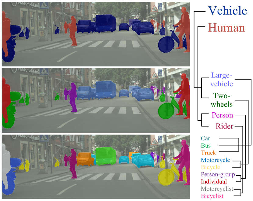
In semantic segmentation literature, surprisingly little is understood about how to accommodate pixel recognition into semantic hierarchies. [80, 83, 89, 45, 56, 43, 81] are rare exceptions that exploit class hierarchies in segmentation networks. Nevertheless, they either focus specifically on the structured organization of human body parts [80, 83, 81], or introduce hierarchy-induced architectural changes to the segmentation network [89, 45, 56, 43], both hindering generality. More essentially, these methods are more aware of making efficient information propagation over the hierarchies (e.g., graph message passing [83, 43, 109], multi-task learning [89]), without imposing tree-structured label dependencies/constraints into prediction and learning.

To mimic human hierarchical visual perception, we propose a novel approach for hierarchical semantic segmentation (HSS). In HSS, classes are not arranged in a “flat” structure, but organized as a tree-shaped hierarchy. Thus each pixel observation is associated to a root-to-leaf path of the class hierarchy (e.g., human$\rightarrow$rider$\rightarrow$bicyclist), capturing general-to-specific relations between classes. Our algorithm, called Hssn, addresses two core issues in HSS, yet untouched before. First, instead of previous structured segmentation models focusing on sophisticated network design, Hssn directly formulates HSS as a pixel-wise multi-label classification task. This allows to easily adapt existing segmentation models to the HSS setting, densely linking the fields of classic hierarchy-agnostic segmentation and HSS together. Second, Hssn makes full use of the class hierarchy in HSS network learning. To make pixel predictions coherent with the class hierarchy, Hssn explores two hierarchy constraints, i.e., i) a pixel sample belonging to a given class must also belong to all its ancestors in the hierarchy, ii) a pixel sample not belonging to a given class must also not belong to all its descendants, as optimization criterion. This leads to a pixel-wise hierarchical segmentation learning strategy, which enforces segmentation predictions to obey the hierarchy structure during training. Hssn further encodes the structured knowledge introduced by the class hierarchy into the pixel embedding space. This leads to a pixel-wise hierarchical representation learning strategy, which inspires tree-induced margin separation for embedding space reshaping. As the hierarchy characterizes the underlying relationships between classes, Hssn is able to enrich pixel embeddings by pulling semantically similar pixels (e.g., bicycle and motorcycle) closer, while pushing semantically dissimilar pixels (e.g., pedestrian and lamppost) farther away. This leads to more efficient learning by discovering and reusing common patterns [27], facilitating hierarchical segmentation eventually. This also allows our model to take different levels of mistakes into consideration. This is essential for some critical systems [7]. Take autonomous driving as an example: mistaking a bicycle for a motorcycle is less of a problem than confusing a pedestrian with a lamppost.

This work represents a solid step towards HSS. Our approach is elegant and principle; it is readily incorporated to arbitrary previous hierarchy-agnostic segmentation networks, with only marginal modification on the segmentation head. We train and test Hssn over four public benchmarks (i.e., Mapillary Vistas 2.0 [58], Cityscapes [18], LIP [44], PASCAL-Person-Part [87]), with different class hierarchies for urban street scene parsing and human semantic parsing. Extensive experimental results with different segmentation network architectures (i.e., DeepLabV3+${}_{\!}$ [13], OCRNet [98], MaskFormer${}_{\!}$ [16]) and backbones (i.e., ResNet-101${}_{\!}$ [34], HRNetV2-W48${}_{\!}$ [79], Swin-Small${}_{\!}$ [49]) verify the generalization and effectiveness of Hssn.

2 Related Work

(Hierarchy-Agnostic) Semantic Segmentation. Semantic segmentation is to partition an image into regions with different semantic categories, which can be viewed as a pixel-wise classification task. Typical solutions for semantic segmentation follow a hierarchy-agnostic setting, where each pixel is assigned to a single label from a set of disjoint semantic categories. In 2015, Long et al. proposed fully con-

volutional networks (FCNs) [50], which are advantageous in end-to-end dense representation modeling, laying the foundation for modern semantic segmentation algorithms. As FCNs suffer from limited visual context with local receptive fields, how to effectively capture cross-pixel relations became the main focus of follow-up studies. Scholars devised many promising solutions, by enlarging receptive${}_{\!}$ fields [105, 19, 93, 97, 10, 13], building image pyramids [46, 33], exploring encoder-decoder architectures [62, 13, 3], utilizing boundary clues [23, 41, 99], or incorporating${}_{\!}$ neural${}_{\!}$ attention${}_{\!}$ [32, 84, 40, 106, 73, 113, 42, 25, 35, 108]. Recently, a new family of semantic segmentation models [90, 69, 107, 16], built upon the full attention (Transformer [76]) architecture, yielded impressive performance, as it overcomes the issues in long-range cross-pixel dependency modeling.

Though impressive, existing semantic segmentation solutions rarely explore the structures between semantic concepts. We take a further step towards class relation aware semantic segmentation, which better reflects the structured nature of our visual world, and echoes the hierarchical reasoning mode of human visual perception. An appealing advantage of our hierarchical solution is that, it can adapt existing class hierarchy-agnostic segmentation architectures, no matter FCN-based or Transformer-like, to the structured setting, in a simple and cheap manner.

Scene${}_{\!}$ Parsing/Hierarchical${}_{\!}$ Semantic${}_{\!}$ Segmentation.${}_{\!}$ Our work is, at a high level, relevant to classical image parsing algorithms [74, 70, 71, 31, 96]. Image parsing has been extensively studied in the pre-deep learning era, dating back to [74]. Image parsing seeks a parse graph that explains visual observation following a “divide-and-conquer”strategy:

a football game image is first parsed into person, sports field, and spectator, which are further decomposed, e.g., person consists of face and body patterns. In the deep learning era, human parsing, as a sub-field of scene parsing, became active. Some recent human parsers explored human part relations, based on the human hierarchy [111, 80, 83, 36, 56, 110]. Only very few efforts [104, 89, 45, 43] are concerned with utilizing structured knowledge to aid the training of general-purpose semantic segmentation networks.

To accommodate the semantic structures imposed by the hierarchy, previous methods tend to greatly change the segmentation network, through the use of different graph neural networks. They hence put all emphasis on how to aggre- gate information over the structured network. Beyond their specific solutions, we propose a general framework for both HSS network design and training. This leads to an elegant view of how to adapt typical segmentation networks to the class hierarchy with only minimal architecture change, and how to involve the hierarchy for regularizing network training, which are core problems yet ignored by prior methods.

Hierarchical Classification. Considering class hierarchies when designing classifiers is a common issue across various machine learning application domains [67], such as text categorization [63], functional genomics [4], and image classification [21, 6]. Depending on whether each datapoint can be assigned a single path or multiple paths in the hierarchy, hierarchy-aware classification can be categorized into hierarchical classification [39, 55, 20, 72] and, a more general setting, hierarchical multi-label classification [8, 85, 29]. In the field of computer vision, exiting efforts for class taxonomy aware image classification can be broadly divided into three groups [7]: i) Label-embedding methods [6, 24, 2, 88] that embed class labels to vectors whose relative locations represent semantic relationships; ii) Hierarchical losses [21, 103, 78, 9, 7] which are designed to inspire the coherence between the prediction and class hierarchy; and iii) Hierarchical architectures [114, 91, 1, 112] that adapt the classifier architecture to the class hierarchy.

Drawing inspiration from these past efforts, we advocate for holistic visual scene understanding through pixel-level hierarchical reasoning. We leverage tree-structured class dependencies as supervision signal to guide hierarchy-coherent pixel prediction and structured pixel embedding.

Hierarchical Embedding. The objective of an embedding algorithm is to organize data samples (e.g., words, images) into an high-dimensional space where their distance reflects their semantic similarity [59]. As semantics are inherently structured, it is necessary to integrate different levels of concept abstraction into representation embedding. Some algorithms directly parameterize the hierarchical embedding space into hierarchical models [86, 78, 60, 57, 14, 92]. While straightforward, they are computationally intensive and have to adjust the network architecture when handling different hierarchies. Some alternatives [28, 94, 5, 38] design hierarchy-aware metric learning objectives [59, 26, 65] to directly shape the embedding space.

With a similar spirit, in this work, we adopt semantic hierarchy-induced margin separation to reinforce pixel representation learning and make prediction less ambiguous.

3 Our Approach

Our goal is to accommodate standard semantic segmentation networks to the HSS problem and then exploit structured class relations in order to generate hierarchy-coherent representations and predictions, and improve performance.${}_{\!}$ Given this goal, we develop${}_{\!}$ Hierarchical${}_{\!}$ Semantic${}_{\!}$ Segmentation${}_{\!}$ Networks${}_{\!}$ (Hssn), a general framework for HSS network design (§3.1) and training (§3.2).

3.1 Hierarchical Semantic Segmentation Networks

Rather than typical segmentation methods treating semantic classes as disjoint labels, in the HSS setting, the underlying dependencies between classes are considered and formalized in a form of a tree-structured hierarchy, $\mathcal{T}_{\!}\!=_{\!}\!(\mathcal{V},\mathcal{E})$. Each node $v_{\!}\!\in_{\!}\!\mathcal{V}_{\!}$ denotes a semantic class/concept, while each edge $(u,v)_{\!}\!\in_{\!}\!\mathcal{E}_{\!}$ encodes the decomposition relationship between two classes, $u,v\!\in\!\mathcal{V}$, i.e., parent node $v$ is a more general, superclass of child node $u$, such as $(u,v)\!=\!(\texttt{bicycle},\texttt{vehicle})$. We assume $(v,v)\!\in\!\mathcal{E}$, thus every class is both a subclass and superclass of itself. The root node of $\mathcal{T}$, i.e., $v^{r}$, denotes the most general class. The leaf nodes, i.e., $\mathcal{V}_{\chi}$, refer to the most fine-grained classes, such as $\mathcal{V}_{\chi\!}\!=\!\{\texttt{tree},\texttt{bicyclist},\cdots\}$ in urban street scene parsing, and $\mathcal{V}_{\chi\!}\!=\!\{\texttt{head},\texttt{leg},\cdots\}$ in human parsing.

For a typical hierarchy-agnostic segmentation network, an encoder $f_{\text{ENC\!}}$ is first adopted to map an image $I$ into a dense feature tensor $\bm{I}\!=\!f_{\text{ENC}}(I)\!\in\!\mathbb{R}^{H\!\times\!W\!\times\!C}$, where $\bm{i}\!\in\!\bm{I}$ is

the embedding of pixel $i_{\!}\!\in_{\!}\!I$. Then a segmentation head $f_{\text{SEG}\!}$ is used to get a score map $\bm{Y}\!=\!\texttt{softmax}(f_{\text{SEG}}(\bm{I}))\!\in\![0,1]^{H\!\times\!W\!\times\!|\mathcal{V}_{\chi\!}|}$${}_{\!}$ w.r.t. the leaf node set $\mathcal{V}_{\chi}$. Given the score vector ${\bm{y}}_{\!}\!=_{\!}\![y_{{v}_{\chi\!}}]_{{v}_{\chi\!}\in\mathcal{V}_{\chi\!\!}}\!\in_{\!}\![0,1]^{|\mathcal{V}_{\chi\!}|\!}$ and groundtruth leaf label $\hat{v}_{\chi\!}\!\in\!\!\mathcal{V}_{\chi\!}$ for pixel $i$, the categorical cross-entropy loss is optimized:​​

$$\small\mathcal{L}^{\text{CCE}}(\bm{y})\!=\!-\log(y_{\hat{v}_{\chi}}).$$ (1)

During inference, pixel $i$ is associated to a single leaf node: $v^{*}_{\chi}\!=\!\operatorname*{arg\,max}_{v_{\chi}}(y_{{v}_{\chi}})$.

To accommodate classic segmentation networks to the HSS setting with minimum change, our Hssn first formulates HSS as a pixel-wise multi-label classification task, i.e., map pixels with their corresponding classes in the hierarchy as a whole. Specifically, only the segmentation head $f_{\text{SEG}\!}$ is modified to predict an augmented score map $\bm{S}\!=\!\texttt{sigmoid}(f_{\text{SEG}}(\bm{I}))\!\in\![0,1]^{H\!\times\!W\!\times\!|\mathcal{V}|}$ w.r.t. the entire class hierarchy $\mathcal{V}$. Given the score vector ${\bm{s}}\!=\![s_{v}]_{{v}\in\mathcal{V}\!}\!\in\![0,1]^{|\mathcal{V}|\!}$ and groundtruth binary label set $\hat{\bm{l}}\!=\![\hat{l}_{v}]_{{v}\in\mathcal{V}\!}\!\in\!\{0,1\}^{|\mathcal{V}|\!}$ for pixel $i$, the binary cross-entropy loss is optimized:​​

$$\small\mathcal{L}^{\text{BCE}}({\bm{s}})=\textstyle\sum\nolimits_{v\in\mathcal{V}}\!-\hat{l}_{v}\!\log(s_{v})\!-\!(1\!-\!\hat{l}_{v})\!\log(1\!-\!s_{v}).$$ (2)

During inference, each pixel $i$ is associated with the top-scoring root-to-leaf path in the class hierarchy $\mathcal{T}$:

$$\small\{v^{*}_{1},\cdots,v^{*}_{|\mathcal{P}|}\}=\!\operatorname*{arg\,max}_{\mathcal{P}\subseteq\mathcal{T}}\textstyle\sum\nolimits_{v_{p}\in\mathcal{P}}s_{v_{p}},$$ (3)

where $\mathcal{P}\!=\!\{v_{1},\cdots,v_{|\mathcal{P}|}\}\!\subseteq\!\mathcal{T}$ denotes a feasible root-to-leaf path of $\mathcal{T}$, i.e., $v_{1\!}\!\in\!\mathcal{V}_{\chi}$, $v_{|\mathcal{P}|\!}\!=\!v^{r}$, and $\forall v_{p},v_{p+1\!}\!\in\!\mathcal{P}\!\Rightarrow\!(v_{p},v_{p+1})\!\in\!\mathcal{E}$. Although Eq. 3 ensures the coherence between pixel-wise prediction and the class hierarchy during the inference stage, there is no any class relation information used for segmentation network training, as the binary cross-entropy loss in Eq. 2 is computed over each class independently. To alleviate this issue, we propose a hierarchy-aware segmentation learning scheme (§3.2), which incorporates the semantic structures into the training of Hssn.

Figure 2: Hierarchy constraints used in our pixel-wise hierarchical segmentation learning (§3.2.1). (a) In the class hierarchy, the filled circles represent the positive classes, while empty circles indicate the negative classes. The positive and negative $\mathcal{T}$-properties are highlighted in the red and blue regions, respectively. (b) The original score vector $\bm{s}$ predicted for the class hierarchy. The predictions which violate the positive and negative $\mathcal{T}$-constraints are highlighted in the red and blue rectangles, respectively. (c) The updated score vector $\bm{p}$, which satisfies the $\mathcal{T}$-constraints. With $\mathcal{L}^{\text{TM}}$, the penalties for the wrong predictions, i.e., ‘0.6’ and ‘0.3’, are increased twice, compared with applying $\mathcal{L}^{\text{BCE}}$ on (b).

3.2 Hierarchy-Aware Segmentation Learning

Our hierarchy-aware segmentation learning scheme includes two major components: i) a pixel-wise hierarchical segmentation learning strategy (§3.2.1) which supervises the segmentation prediction $\bm{S}$ in a hierarchy-coherent manner, and ii) a pixel-wise hierarchical representation learning strategy (§3.2.2) that makes hierarchy-induced margin separation for reshaping the pixel embedding space $f_{\text{ENC}}$.

3.2.1 Pixel-Wise Hierarchical Segmentation Learning

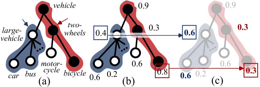
For each pixel, the assigned labels are hierarchically consistent if they satisfy the following two properties (Fig.​ 2):

Definition 3.2.1 (Positive $\mathcal{T}$-Property).

For each pixel, if a class is labeled positive, all its ancestor nodes (i.e., superclasses) in $\mathcal{T}$ should be labeled positive.

Definition 3.2.2 (Negative $\mathcal{T}$-Property).

For each pixel, if a class is labeled negative, all its child nodes (i.e., subclasses) in $\mathcal{T}$ should be labeled negative.

The first property, also known as $\mathcal{T}$-property [8], was explored in some hierarchical classification work [77, 85, 29], while the second property is ignored. Actually, these two properties are complementary and crucial for consistent hierarchical prediction. Specifically, to incorporate these two label consistency properties into the supervision of Hssn, we further derive the following two hierarchy constraints w.r.t. per-pixel prediction, i.e., ${\bm{s}}\!=\![s_{v}]_{{v}\in\mathcal{V}\!}\!\in\![0,1]^{|\mathcal{V}|}$:

Definition 3.2.3 (Positive $\mathcal{T}$-Constraint).

For each pixel, if $v$ class is labeled positive, and $u$ is an ancestor node (i.e., superclass) of $v$, it should hold that $s_{v}\!\leq\!s_{u}$.

Definition 3.2.4 (Negative $\mathcal{T}$-Constraint).

For each pixel, if $v$ class is labeled negative, and $u$ is a child node (i.e., subclass) of $v$, it should hold that $1-s_{v}\!\leq\!1-s_{u}$.

With the positive $\mathcal{T}$-constraint (cf. Def. 3.2.3), the positive $\mathcal{T}$-property (cf. Def. 3.2.1) can be always guaranteed. Similar conclusion is also hold for the negative $\mathcal{T}$-constraint (cf. Def. 3.2.4) and negative $\mathcal{T}$-property (cf. Def. 3.2.2).

Tree-Min Loss. To ensure the satisfaction of the two hierarchy constraints, we estimate a hierarchy-coherent score map $\bm{P}\!\in\![0,1]^{H\!\times\!W\!\times\!|\mathcal{V}|}$ from $\bm{S}$. For pixel $i$, the updated score vector $\bm{p}\!=\![p_{v}]_{{v}\in\mathcal{V}\!}\!\in\![0,1]^{|\mathcal{V}|}$ in $\bm{P}$ is given as:

$$\small\!\!\!\left\{\begin{aligned} p_{v}&\!=\min_{u\in\mathcal{A}_{v}}(s_{u})~{}~{}~{}~{}~{}~{}~{}~{}~{}~{}~{}~{}~{}~{}~{}~{}~{}~{}~{}~{}~{}~{}~{}~{}~{}~{}~{}~{}~{}~{}~{}~{}~{}~{}~{}\!\text{if~{}~{}}\hat{l}_{v}\!=\!1,\!\\[-2.71246pt] 1\!-\!p_{v}&\!=\!\min_{u\in\mathcal{C}_{v}}(1\!-\!s_{u})\!=\!1\!-\!\max_{u\in\mathcal{C}_{v}}(s_{u})~{}~{}~{}~{}~{}~{}\!\text{if~{}~{}}\hat{l}_{v}\!=\!0,\!\end{aligned}\right.$$ (4)

where $\mathcal{A}_{v}$ and $\mathcal{C}_{v\!}$ denote the superclass and subclass sets of $v$ in $\mathcal{T}$ respectively, and $\bm{s}\!=\![s_{v}]_{{v}\in\mathcal{V}\!}\!\in_{\!}\!\bm{S}$ refers to the original score vector of pixel $i$. Note that, according to our definition $(v,v)\in\mathcal{E}$ (cf. §3.1), we have $v\!\in\!\mathcal{A}_{v}$ and $v\!\in\!\mathcal{C}_{v}$. With Eq. 4, the pixel-wise prediction $\bm{p}$ is guaranteed to always satisfy the hierarchy constraints (cf. Defs. 3.2.3 and 3.2.4).

We thus build a hierarchical segmentation training objective, i.e., tree-min loss, to replace $\mathcal{L}^{\text{BCE}}({\bm{s}})$ in Eq. 2:

$$\!\!\!\mathcal{L}^{\text{TM}\!}(\bm{p}) =\textstyle\sum\limits_{v\in\mathcal{V}}-\hat{l}_{v}\!\log(p_{v})-(1-\hat{l}_{v})\!\log(1\!-\!p_{v}),\!\!\!$$ (5)

$$=\textstyle\sum\limits_{v\in\mathcal{V}}-\hat{l}_{v}\!\log(\min\limits_{u\in\mathcal{A}_{v}}({s}_{u}))-$$

$$~{}~{}~{}~{}~{}~{}~{}~{}~{}~{}~{}~{}~{}(1-\hat{l}_{v})\!\log(1-\max_{u\in\mathcal{C}_{v}}(s_{u})).\!\!\!$$

Compared with $\mathcal{L}^{\text{BCE}}(\bm{s})$, $\mathcal{L}^{\text{TM}}(\bm{p})$ is more favored as the structured score distribution $\bm{p}$ is constructed by strictly following the hierarchy constraints (cf. Eq. 4), and hence the violation of the hierarchy properties (i.e., any undesired prediction of $\bm{p})$ can be explicitly penalized (see Fig.​ 2(c)).

Figure 3: Effect of $\mathcal{L}^{\text{BCE}}$ in Eq. 2 (top) vs $\mathcal{L}^{\text{FTM}}$ in Eq. 6 (bottom).

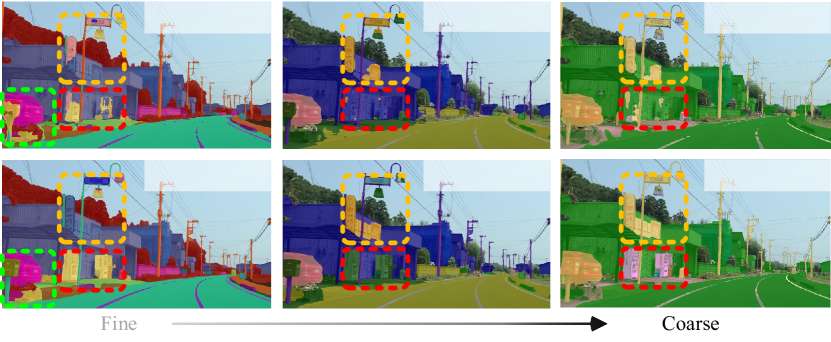
Focal Tree-Min Loss. Inspired by the focal loss [47], we add a modulating factor to the tree-min loss (cf. Eq. 5), so as to reduce the relative loss for well-classified pixel samples and focus on those difficult ones:

$$\!\!\!\!\!\!\!\!\!\mathcal{L}^{\text{FTM}\!}(\bm{p}) \!=\!\!\!\textstyle\sum\limits_{v\in\mathcal{V}}\!\!-\hat{l}_{v}(1\!-\!p_{v\!})^{\gamma\!}\log(p_{v\!})\!-\!(1\!-\!\hat{l}_{v\!})(p_{v\!})^{\gamma\!}\log(1\!-\!p_{v\!}),\!\!\!\!\!\!$$ (6)

$$\!=\!\!\!\textstyle\sum\limits_{v\in\mathcal{V}}\!\!-\hat{l}_{v}(1\!-\!\min\limits_{u\in\mathcal{A}_{v}}({s}_{u}))^{\gamma\!}\log(\min\limits_{u\in\mathcal{A}_{v}}({s}_{u}))-\!\!\!$$

$$~{}~{}~{}~{}~{}~{}~{}~{}(1\!-\!\hat{l}_{v})(\max_{u\in\mathcal{C}_{v}}(s_{u}))^{\gamma\!}\log(1\!-\!\max_{u\in\mathcal{C}_{v}}(s_{u})),\!\!\!\!\!\!$$

where $\gamma\!\geq\!0$ is a tunable focusing parameter controling the rate at which easy classes are down-weighted. When $\gamma\!=\!0$, $\mathcal{L}^{\text{FTM}}(\bm{p})$ is equivalent to $\mathcal{L}^{\text{TM}}(\bm{p})$. Fig. 3 shows representative visual effects of $\mathcal{L}^{\text{FTM}}$ against $\mathcal{L}^{\text{BCE}}$. We see that $\mathcal{L}^{\text{FTM}}$ yields more precise and coherent results. In §4.4, we provide quantitative comparison results for $\mathcal{L}^{\text{BCE}}(\bm{s})$ (cf. Eq. 2), $\mathcal{L}^{\text{TM}}(\bm{p})$ (cf. Eq. 5), and $\mathcal{L}^{\text{FTM}}(\bm{p})$ (cf. Eq. 6).

3.2.2 ${}_{\!}$Pixel-Wise Hierarchical Representation Learning${}_{\!\!\!}$

Through mapping pixels with their corresponding semantic classes in the hierarchy $\mathcal{T}$ as a whole (cf. §3.1), we exploit intrinsic properties of $\mathcal{T}$ (cf. Defs. 3.2.1-3.2.2) as constraints (cf. Defs. 3.2.3-3.2.4) to encourage hierarchy-coherent segmentation prediction $\bm{S}$ (cf. Eqs. 5-6). As the class hierarchy provides rich semantic relations among categories over different levels of concept abstraction, next we will exploit such structured knowledge to reshape the pixel embedding space $f_{\text{ENC}}$, so as to generate more efficient pixel representations and improve final segmentation performance.

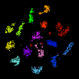
With this purpose, we put forward a margin based pixel-wise hierarchical representation learning strategy, where the learned pixel embeddings are well separated with structured margins imposed by the class hierarchy $\mathcal{T}$. Specifically, for any pair of labels $u,v\!\in\!\mathcal{V}$, let $\psi(u,v)$ denote their distance in the tree $\mathcal{T}$. That is, $\psi(u,v)$ is defined as the length (in edges) of the shortest path between $u$ and $v$ in $\mathcal{T}$. The distance function $\psi(\cdot,\cdot)$ is in fact a semantic similarity metric defined over $\mathcal{T}$ [20]; it is a non-negative and symmetric function, $\psi(v,v)\!=\!0$, $\psi(u,v)\!=\!\psi(v,u)$, and the triangle inequality always holds with equality.

In Hssn, the structured margin constraints are defined by the tree distance $\psi(\cdot,\cdot)$, leading to a tree-triplet loss. This loss is optimized on a set of pixel triplets $\{i,i^{+},i^{-\!}\}$, where $i,i^{+},i^{-\!}$ are anchor, positive and negative pixel samples, respectively. $\{i,i^{+},i^{-}\}$ are sampled from the whole training batch, such that $\psi(\hat{v}_{\chi},\hat{v}^{+}_{\chi})\!<\!\psi(\hat{v}_{\chi},\hat{v}^{-}_{\chi})$, where $\hat{v}_{\chi}$, $\hat{v}^{+}_{\chi},\hat{v}^{-\!}_{\chi\!}\!\in\!\mathcal{V}_{\chi\!}$ are the groundtruth leaf labels of $i$, $i^{+}$, and $i^{-}$, respectively. As such, in our tree-triplet loss, the positive samples are more semantically similar to the anchor pixels (i.e., closer in $\mathcal{T}$), compared with the negative pixels. Note that this is different from the classic, hierarchy-agnostic triplet loss [66], where the anchor and positive samples are from the same class, while the anchor and negative samples are from different classes, i.e., $\hat{v}_{\chi}\!=\!\hat{v}^{+}_{\chi}$, and $\hat{v}_{\chi}\!\neq\!\hat{v}^{-}_{\chi}$. With a valid training triplet $\{i,i^{+},i^{-\!}\}$, our loss is given as:

$$\mathcal{L}^{\text{TT}}(\bm{i},\bm{i}^{+},\bm{i}^{-\!})=\max\{\langle\bm{i},\bm{i}^{+}\rangle-\langle\bm{i},\bm{i}^{-}\rangle+m,0\},$$ (7)

where $\bm{i},\bm{i}^{+},\bm{i}^{-\!}\!\in\!\mathbb{R}^{C}$ are the embeddings of $i$, $i^{+}$, and $i^{-}$, respectively, obtained from the encoder $f_{\text{ENC}}$, $\langle\cdot,\cdot\rangle$ is a distance function to measure the similarity of two inputs; we use the cosine distance, i.e., $\langle\bm{x},\bm{y}\rangle\!=\!\frac{1}{2}(1\!-\!\frac{\bm{x}\cdot\bm{y}}{\|\bm{x}\|\|\bm{y}\|})\!\in\![0,1]$. The margin $m$ forces the gap of $\langle\bm{i},\bm{i}^{-}\rangle$ and $\langle\bm{i},\bm{i}^{+}\rangle$ larger than $m$. When the gap is larger than $m$, the loss value would be zero. The separation margin $m$ is determined as:

$$\small m =m_{\varepsilon}+0.5m_{\tau}$$ (8)

$$m_{\tau} =(\psi(\hat{v}_{\chi},\hat{v}^{-\!}_{\chi})-\psi(\hat{v}_{\chi},\hat{v}^{+\!}_{\chi}))/2D,$$

where $m_{\varepsilon}\!\!=\!\!0.1$ is set as a constant for the tolerance of the intra-class variance, i.e., maximum intra-class distance, $m_{\tau}\!\in\![0,1]$ is a dynamic violate margin, which is computed according to the semantic relationships among $i$, $i^{+}$, and $i^{-\!}$ over the class hierarchy $\mathcal{T}$, and $D$ refers to the height of $\mathcal{T}$.

Figure 4: Visualization of the hierarchical embedding space $f_{\text{ENC}}$ learned on Mapillary Vistas 2.0 [58] (§3.2.2). The different colors correspond to different categories. It can be seen that, with $\mathcal{L}^{\text{TT}}$, $f_{\text{ENC}}$ (middle) nicely embraces the hierarchical semantic structures (right), in comparison with the one without $\mathcal{L}^{\text{TT}}$ (left).

Eq. 7 encourages $f_{\text{ENC}}$ as a hierarchically-structured embedding space (Fig. 4): pixels with similar semantics (i.e.,${}_{\!}$ nearby in $\mathcal{T}$) are pushed closer than those with dissimilar semantics (i.e.,${}_{\!}$ faraway in $\mathcal{T}$), guided by the hierarchy-induced margin $m$. Related experiments are given in §4.4.

3.3 Implementation Detail

Network Architecture. Hssn is a general HSS framework; it is readily applied to any hierarchy-agnostic segmentation${}_{\!}$ models. i) The segmentation encoder $f_{\text{ENC}}$ (§3.1) maps each input image $I$ into a dense feature $\bm{I}\!\in\!\mathbb{R}^{H\!\times\!W\!\times\!C}$, and can be implemented as any backbone networks. In §4, we experiment with two CNN-based (i.e., ResNet-101${}_{\!}$ [34] and HRNetV2-W48${}_{\!}$ [79]) and a Transformer-based (i.e., Swin-Transformer [49]) backbones. ii) The segmentation head $f_{\text{SEG}}$ (§3.1) projects $\bm{I}$ into a structured score map $\bm{S}\!\in\!\mathbb{R}^{H\!\times\!W\!\times\!|\mathcal{V}|}$ for all the classes in $\mathcal{V}$. Segmentation heads used in recent segmentation models (i.e., DeepLabV3+${}_{\!}$ [13], OCRNet${}_{\!}$ [98], MaskFormer${}_{\!}$ [16]) are used and modified.

Training Objective. Hssn is end-to-end trained by minimizing the combinatorial loss of our focal tree-min loss ($\mathcal{L}^{\text{FTM}}$ in Eq. 6) and tree-triplet loss ($\mathcal{L}^{\text{TT}}$ in Eq. 7): $\mathcal{L}^{\text{FTM}}+\beta\mathcal{L}^{\text{TT}}$, where the coefficient $\beta\!\in\![0,0.5]$ is scheduled following a cosine annealing policy​ [51]. The focusing parameter $\gamma$ in $\mathcal{L}^{\text{FTM}\!}$ is set as 2. Furthermore, following the common practice in metric learning, a projection function $f_{\text{PROJ}}$ is used in $\mathcal{L}^{\text{TT}}$. It maps each pixel embedding $\bm{i}$ into a 256-$d$ vector. $f_{\text{PROJ}}$ consists of two $1\!\times\!1$ convolutional layers and one ReLU between them, and is discarded after training, causing no extra computational cost in deployment.

Inference.${}_{\!}$ For${}_{\!}$ each${}_{\!}$ pixel,${}_{\!}$ the${}_{\!}$ label${}_{\!}$ assignment${}_{\!}$ follows${}_{\!}$ Eq.${}_{\!}$ 3.${}_{\!\!\!}$

Figure 5: ${}_{\!}$Visual${}_{\!}$ results${}_{\!}$ (§4.3)${}_{\!}$ on${}_{\!}$ Mapillary${}_{\!}$ Vistas${}_{\!}$ $2.0$​ [58]${}_{\!}$ val${}_{\!}$ (left) and${}_{\!}$ Cityscapes​ [18]${}_{\!}$ val${}_{\!}$ (right).${}_{\!}$ Top:${}_{\!}$ MaskFormer,${}_{\!}$ Bottom:${}_{\!}$ Hssn.

4 Experiment

4.1 Experimental Setup

Datasets. We conduct experiments on two popular urban street scene parsing datasets [58, 18] and two human body parsing datasets [87, 44]. The corresponding class hierarchies are either the officially provided ones [58, 18] or generated by following the conventions [87, 44].

• Mapillary${}_{\!}$ Vistas${}_{\!}$ 2.0 [58] is an urban egocentric street-view dataset with high-resolution images. It contains $18,\!000$, $2,\!000$ and $5,\!000$ images for train, val and test, respectively. It provides annotations for $144$ semantic concepts, which are organized in a three-level hierarchy, covering $4/16/124$ concepts, respectively.

• Cityscapes [18] contains $5,\!000$ elaborately annotated urban scene images, which are split into $2,\!975/500/1,\!524$ for train/val/test. It is associated with $19$ fine-grained concepts, which are grouped into $6$ super-classes.

• PASCAL-Person-Part [87] has $1,\!716$ and $1,\!817$ images for train and test, with precise annotations for $6$ human parts. Following [80, 83], we group $20$ fine-grained parts (e.g., head, left-arm) into two superclasses upper-body and lower-body, which are further combined ito full-body.

• LIP [44] includes $50,\!462$ single-person images gathered from real-world scenarios, with $30,\!462/10,\!000/10,\!000$ for $\texttt{train}/\texttt{val}/\texttt{test}$ splits. The hierarchy is similar to the one in PASCAL-Person-Part, but the leaf layer has $19$ fine-grained semantic parts.

Training. For fair comparison, we follow [102, 80, 105, 13] to set the training hyper-parameters. Specifically, for CNN-based models, we use SGD as the optimizer with base learning rate 1e-2, momentum $0.9$ and weight decay 1e-4. For Transformer-based models, we use AdamW [52] with base learning rate 6e-5 and weight decay $0.01$. The learning rate is scheduled by the polynomial annealing policy [11]. All backbones are initialized using the weights pre-trained on ImageNet-$1$K [22], while the remaining layers are randomly initialized. During training, we use standard data augmentation techniques, i.e., horizontal flipping and random scaling with a ratio between $0.5$ and $2.0$. We train $240$K and $80$K iterations for Mapillary Vistas $2.0$ and Cityscapes, with batch size $8$ and crop size $512\!\times\!1024$. For PASCAL-Person-Part and LIP, we use batch size $16$ and crop size $480\!\times\!480$, and train models for $80$K and $160$K iterations, respectively.

Testing. The inference follows Eq.${}_{\!}$ 3. As in [35, 16, 98, 36, 83, 80], we report the segmentation scores at multiple scales ($\{0.5,0.75,1.0,1.25,1.5,1.75\}_{\!}$) with horizontal flipping.

Evaluation Metric. The mean intersection-over-union (mIoU) is adopted for evaluation. Particularly, we report the average score, i.e., mIoU^l, for classes in each hierarchy level $l$ independently. For reference, we also report the scores of each level for hierarchy-agnostic methods. The results of each non-leaf layer are obtained by merging the segmentation predictions of its subclasses together.

Method		Backbone	$\text{mIoU}^{3}$$\uparrow$	$\text{mIoU}^{2}$$\uparrow$	$\text{mIoU}^{1}$$\uparrow$
DeepLabV3+ [13]​​	​​[ECCV18]	ResNet-101	81.86	68.17	37.43
Seamless [61]​​	​​[CVPR19]	ResNet-101	-	-	38.17
OCRNet [98]​​	​​[ECCV20]	HRNet-W48	83.19	69.32	38.26
HMSANet [83]​​	​​[ArXiv19]	HRNet-W48	84.63	70.71	39.53
MaskFormer [16]​​	​​[NeurIPS21]	ResNet-101	84.56	70.82	39.60
MaskFormer [16]​​	​​[NeurIPS21]	Swin-Small	87.93	73.88	42.16
DeepLabV3+		ResNet-101	85.27	71.40	40.16
Hssn OCRNet		HRNet-W48	86.46	72.34	41.13
MaskFormer		Swin-Small	90.02	75.81	43.97

Table 1: Hierarchical semantic segmentation results${}_{\!}$ (§4.2) on the val set of Mapillary Vistas $2.0$ [58].

Method		Backbone	$\text{mIoU}^{2}$$\uparrow$	$\text{mIoU}^{1}$$\uparrow$
DeepLabV2 [10]​​	​​[CVPR17]	ResNet-101	-	70.22
PSPNet [105]​​	​​[CVPR17]	ResNet-101	-	80.91
PSANet [106]​​	​​[ECCV18]	ResNet-101	-	80.96
PAN [40]​​	​​[ArXiv18]	ResNet-101	-	81.12
DeepLabV3+ [13]​​	​​[ECCV18]	ResNet-101	92.16	82.08
DANet [25]​​	​​[CVPR19]	ResNet-101	-	81.52
Acfnet [100]​​	​​[ICCV19]	ResNet-101	-	81.60
CCNet [35]​​	​​[ICCV19]	ResNet-101	-	81.08
HANet [17]​​	​​[CVPR20]	ResNet-101	-	81.82
HRNet [79]​​	​​[TPAMI20]	HRNet-W48	92.12	81.96
OCRNet [98]​​	​​[ECCV20]	HRNet-W48	92.57	82.33
MaskFormer [16]​​	​​[NeurIPS21]	Swin-Small	92.96	82.57
DeepLabV3+		ResNet-101	93.31	83.02
Hssn OCRNet		HRNet-W48	93.92	83.37
MaskFormer		Swin-Small	94.39	83.74

Table 2: Hierarchical${}_{\!}$ semantic segmentation results${}_{\!}$ (§4.2) on the val set of Cityscapes [18].

Method		Head	Torso	U-Arm	L-Arm	U-Leg	L-Leg	U-Body	L-Body	F-Body	B.G.	$\text{mIoU}^{3}$$\uparrow$	$\text{mIoU}^{2}$$\uparrow$	$\text{mIoU}^{1}$$\uparrow$
DeepLabV3+ [13]​​​	​​​[ECCV18]​	87.02	72.02	60.37	57.36	53.54	48.52	90.07	65.88	93.02	96.07	94.55	84.01	67.84
SPGNet [15]​​​	​​​[ICCV19]​	87.67	71.41	61.69	60.35	52.62	48.80	-	-	-	95.98	-	-	68.36
PGN [30]​​​	​​​[CVPR19]​	90.89	75.12	55.83	64.61	55.42	41.57	-	-	-	95.33	-	-	68.40
CNIF [80]​​​	​​​[ICCV19]​	88.02	72.91	64.31	63.52	55.61	54.96	91.82	66.56	94.33	96.02	95.18	84.80	70.76
SemaTree [36]​​​	​​​[ECCV20]​	89.15	74.76	63.90	63.95	57.53	54.62	92.36	67.13	95.11	96.84	95.98	85.44	71.59
HHP [83]​​​	​​​[CVPR20]​	89.73	75.22	66.87	66.21	58.69	58.17	93.44	68.02	96.77	96.94	96.86	86.13	73.12
BGNet [102]​​​	​​​[ECCV20]​	90.18	77.44	68.93	67.15	60.79	59.27	-	-	-	97.12	-	-	74.42
PCNet [101]​​​	​​​[CVPR20]​	90.04	76.89	69.11	68.40	60.78	60.14	-	-	-	96.78	-	-	74.59
Hssn DeepLabV3+		90.19	78.72	70.67	69.71	61.15	60.44	95.86	71.56	98.20	97.18	97.69	88.20	75.44

Table 3: Hierarchical human parsing results (§4.2) on PASCAL-Person-Part [87] test. All models use ResNet-101 as the backbone.

Method		Backbone	$\text{mIoU}^{3}$$\uparrow$	$\text{mIoU}^{2}$$\uparrow$	$\text{mIoU}^{1}$$\uparrow$
SegNet [3]​​	​​[TPAMI17]​	ResNet-101	-	-	18.17
FCN-8s [50]​​	​​[CVPR15]​	ResNet-101	-	-	28.29
DeepLabV2 [10]​​	​​[CVPR17]​	ResNet-101	-	-	41.64
Attention [12]​​	​​[CVPR16]​	ResNet-101	-	-	42.92
MMAN [54]​​	​​[ECCV18]​	ResNet-101	-	-	46.93
DeepLabV3+​ [13]​​	​​[ECCV18]​	ResNet-101	88.13	83.97	52.28
CE2P [64]​​	​​[AAAI19]​	ResNet-101	-	-	53.10
BraidNet [48]​​	​​[ACMMM19]​	ResNet-101	-	-	54.42
SemaTree [36]​​	​​[ECCV20]​	ResNet-101	90.78	87.12	54.73
BGNet [102]​​	​​[ECCV20]​	ResNet-101	-	-	56.82
PCNet [101]​​	​​[CVPR20]​	ResNet-101	-	-	57.03
CNIF [80]​​	​​[ICCV19]​	ResNet-101	95.92	91.83	57.74
HRNet [79]​​	​​[TPAMI20]​	HRNet-W48	95.53	91.21	57.23
OCRNet [98]​​	​​[ECCV20]​	HRNet-W48	96.78	92.56	58.47
HHP [83]​​	​​[CVPR20]​	ResNet-101	97.41	93.43	59.25
Hssn DeepLabV3+		ResNet-101	98.86	94.75	60.37

Table 4: ${}_{\!}$Hierarchical${}_{\!}$ human${}_{\!}$ parsing${}_{\!}$ results (§4.2) on LIP val.${}_{\!\!\!}$

4.2 Quantitative Results

Mapillary Vistas 2.0 [58]. Table 1 presents comparisons of our Hssn against several top-leading semantic segmentation models on Mapillary Vistas $2.0$ val. With the standard ResNet-101 as the backbone, Hssn outperforms the famous DeepLabV3+ [13] by solid margins across all three levels (2.69%/3.21%/3.40%). Consistent gains are also observed for a more recent segmentation model (i.e., MaskFormer [16]), which relies on a heavy Transformer-based decoder. In addition, our Hssn further improves the performance when using more advanced CNN-based (i.e., HRNetV2-W48) or Transformer-based (i.e., Swin-Small) backbones. Concretely, it outperforms OCRNet [98] by 2.87%/3.02%/3.27% and MaskFormer [16] by 1.81%/ 1.93%/2.09% across the three levels. Hssn, with Swin-Small as the backbone, establishes a new state-of-the-art. These results clearly demonstrate the efficacy of our hierarchical semantic segmentation framework.

Figure 6: Visual results (§4.3) on LIP [44] val (left) and PASCAL-Person-Part [87] test (right). Top: DeepLabV3+, Bottom: Hssn.

Cityscapes [18]. Table 2 compares our Hssn with several competitive models on Cityscapes val. Despite that the dataset has relatively simple semantic hierarchy and has been comprehensively benchmarked, our model still leads to appealing improvements. In particular, Hssn outperforms the top-leading MaskFormer [16] by 1.17%/1.43% in terms of mIoU¹ and mIoU² when using Swin-Small as the backbone. Similar gains are obtained when applying CNN-based backbones (i.e., ResNet-101 and HRNet-W48).

PASCAL-Person-Part [87]. Table 3 lists the detailed results on PASCAL-Person-Part test. Note that all the models use ResNet-101 as the backbone. As seen, our Hssn achieves the best performance for all human parts and hierarchical levels. Remarkably, Hssn outperforms all existing hierarchical human parsers (i.e., HHP [83], SemaTree [36] and CNIF [80]) by significant margins. Results on this dataset are particularly impressive since it includes a very small number (i.e., $1,\!713$) of training samples.

LIP [44]. In Table 4, we compare Hssn with state-of-the-art human semantic parsing models on LIP val. As observed, our model provides a considerable performance gain against the leading hierarchy-aware human parser (i.e., HHP [83]) across all three levels ($\textbf{1.12\%}/\textbf{1.32\%}/\textbf{1.45\%}$). These results support our motivation of exploiting structured label constraints and structured representation learning rather than only focusing on structured feature fusion.

4.3 Qualitative Results

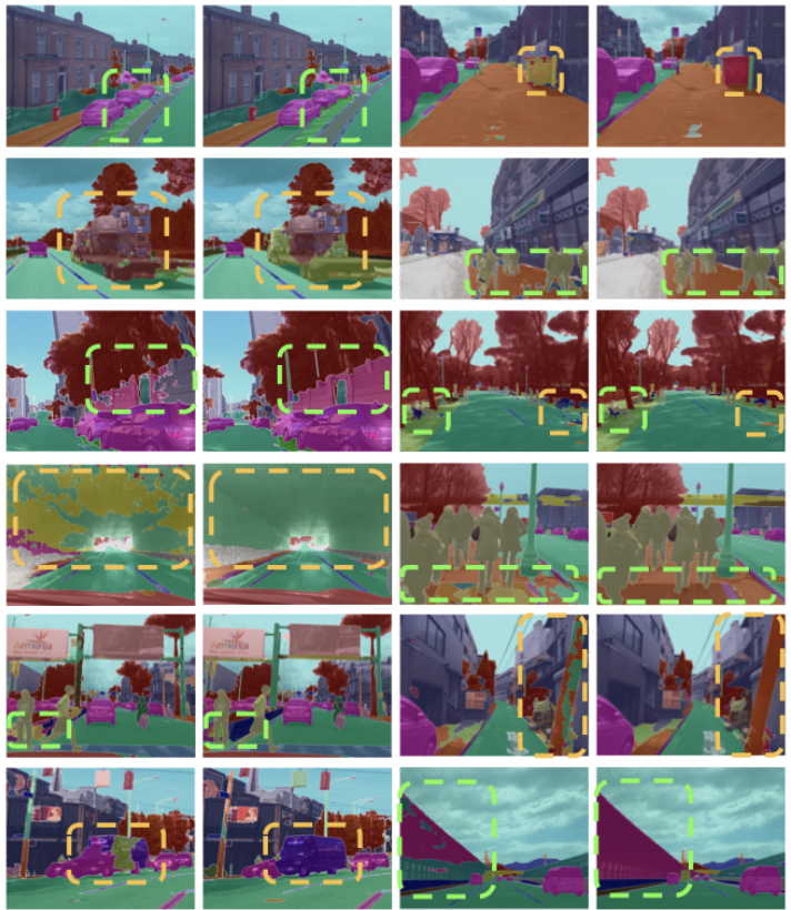
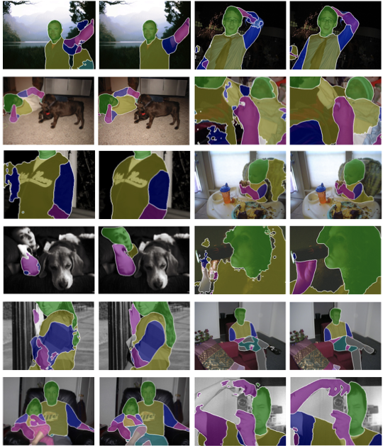
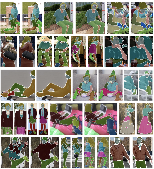
Fig. 5 and Fig. 6 depict representative visual results on four datasets. As seen, Hssn yields more precise segmentation results in comparison with some top-performing methods (i.e., MaskFormer in Fig. 5 and DeepLabV3+ in Fig. 6), and shows strong robustness to various challenging scenarios with occlusions, small objects and densely arranged targets, etc. Moreover, as shown in the last column of Fig. 5, MaskFormer makes a severe mistake that misclassifies a part of background structure as truck. In contrast, benefiting from hierarchy-aware segmentation learning, Hssn naturally address the issue of mistake severity, i.e., distinguish significantly different concepts with larger margins.

4.4 Diagnostic Experiment

To gain more insights into Hssn, we conduct a set of ablative studies on Mapillary Vistas 2.0 [58] and Pascal-Person-Part [87], with ResNet-101 as the backbone.

Key Component Analysis. First, we investigate the essential designs in Hssn, i.e., hierarchical segmentation learning (§3.2.1) with $\mathcal{L}^{\text{FTM}\!}$ (cf.${}_{\!}$ Eq. 6) and hierarchical representation learning (§3.2.2) with $\mathcal{L}^{\text{TT}\!}$ (cf.${}_{\!}$ Eq. 7). The results are summarized in Table 5. The first row refers to a hierarchy-agnostic baseline that only concerns the leaf nodes and is trained using the categorical cross-entropy loss $\mathcal{L}^{\text{CCE}}$ (cf.${}_{\!}$ Eq. 1). Three crucial conclusions can be drawn. First, our $\mathcal{L}^{\text{FTM}\!}$ leads to significant performance improvements against the baseline across all the metrics on both datasets. This evidences that our hierarchical segmentation learning strategy is able to produce hierarchy-coherent predictions. Second, we also observe compelling gains by incorporating $\mathcal{L}^{\text{TT}}$ into the baseline. This proves the importance of hierarchical representation learning. Third, our full model achieves the best performance by combining our $\mathcal{L}^{\text{FTM}}$ and $\mathcal{L}^{\text{TT}}$ together, confirming the necessity of joint hierarchical segmentation and embedding learning.

Focal Tree-Min Loss. We next examine the design of our focal tree-min loss $\mathcal{L}^{\text{FTM}}$ (cf.${}_{\!}$ Eq. 6). As shown in Table 6, we compare $\mathcal{L}^{\text{FTM}}$ with four different losses, i.e., categorical cross-entropy loss $\mathcal{L}^{\text{CCE}}$ (cf.${}_{\!}$ Eq. 1), binary cross-entropy loss $\mathcal{L}^{\text{BCE}}$ (cf.${}_{\!}$ Eq. 2), focal loss [47], and our tree-min loss $\mathcal{L}^{\text{TM}}$ (cf.${}_{\!}$ Eq. 5). We can find that our $\mathcal{L}^{\text{TM}}$ generates impressive results, and $\mathcal{L}^{\text{FTM}}$ is even better than $\mathcal{L}^{\text{TM}}$. Then, in Table 7, we analyze the impact of the focusing parameter $\gamma$ in $\mathcal{L}^{\text{FTM}}$. As seen, the performance progressively improves as $\gamma$ is increased, and the gain becomes marginal when $\gamma\!=\!2$. Hence, we choose $\gamma\!=\!2$ by default.

$\mathcal{L}^{\text{FTM}}$	$\mathcal{L}^{\text{TT}}$	Mapillary Vistas 2.0			Pascal-Person-Part
Eq. 6	Eq. 7	$\text{mIoU}^{3}$$\uparrow$	$\text{mIoU}^{2}$$\uparrow$	$\text{mIoU}^{1}$$\uparrow$	$\text{mIoU}^{3}$$\uparrow$	$\text{mIoU}^{2}$$\uparrow$	$\text{mIoU}^{1}$$\uparrow$
		81.86	68.17	37.43	93.58	83.04	67.84
✓		84.17	69.62	39.17	96.33	86.72	72.89
	✓	83.06	68.61	38.29	95.92	86.03	72.27
✓	✓	85.27	71.40	40.16	97.69	88.20	75.44

Table 5: Analysis of essential components on Mapillary Vistas $2.0$ [58] val and PASCAL-Person-Part [87] test (§4.4).

	Mapillary Vistas 2.0			Pascal-Person-Part
Loss	$\text{mIoU}^{3}$$\uparrow$	$\text{mIoU}^{2}$$\uparrow$	$\text{mIoU}^{1}$$\uparrow$	$\text{mIoU}^{3}$$\uparrow$	$\text{mIoU}^{2}$$\uparrow$	$\text{mIoU}^{1}$$\uparrow$
CCE	81.86	68.17	37.43	93.58	83.04	67.84
BCE	81.56	67.61	37.26	93.12	82.55	67.38
Focal	82.63	68.48	38.09	94.07	83.66	68.42
TM	83.48	69.13	38.69	95.32	85.99	72.17
FTM	84.17	69.62	39.17	96.33	86.72	72.89
Full	85.27	71.40	40.16	97.69	88.20	75.44

Table 6: Analysis of focal tree-min loss $\mathcal{L}^{\text{FTM}}$ on Mapillary Vistas $2.0$ [58] val and PASCAL-Person-Part [87] test (§4.4).

Tree-Triplet Loss. We further investigate the design of our tree-triplet loss $\mathcal{L}^{\text{TT}\!}$ (cf.${}_{\!}$ Eq. 7). In Table 8, “Vanilla” refers to the vanilla triplet loss with a constant margin [66]. By constructing hierarchy-aware triplet samples, our tree-triplet loss $\mathcal{L}^{\text{TT}}$ (also with a constant margin) outperforms “Vanilla”. The gains become larger when further applying the hierarchy-induced margin constraint. These results confirm the designs of our tree-triplet loss. Finally, we assess the impact of the distance measurement $\langle\cdot,\cdot\rangle$ used in $\mathcal{L}^{\text{TT}\!}$. We study Cosine and Euclidean distances. Table 9 shows that Cosine distance performs much better than Euclidean distance, corroborating relevant observations in [59, 26, 65].

$\gamma$	Mapillary Vistas 2.0			Pascal-Person-Part
Eq. 6	$\text{mIoU}^{3}$$\uparrow$	$\text{mIoU}^{2}$$\uparrow$	$\text{mIoU}^{1}$$\uparrow$	$\text{mIoU}^{3}$$\uparrow$	$\text{mIoU}^{2}$$\uparrow$	$\text{mIoU}^{1}$$\uparrow$
$0$	84.47	70.24	39.52	96.90	87.56	74.84
$0.2$	84.53	70.38	39.62	97.17	87.71	74.91
$0.5$	84.85	70.61	39.72	97.23	87.68	74.94
$1.0$	85.11	70.95	39.94	97.44	87.97	75.20
$2.0$	85.27	71.40	40.16	97.69	88.20	75.44
$5.0$	84.92	70.07	39.40	96.84	87.25	74.65

Table 7: Analysis of $\gamma$ for $\mathcal{L}^{\text{FTM}}$ (Eq. 6) on Mapillary Vistas $2.0$ [58] val and PASCAL-Person-Part [87] test (§4.4).

Triplet	Margin	Mapillary Vistas 2.0			Pascal-Person-Part
Loss	$m$	$\text{mIoU}^{3}$$\uparrow$	$\text{mIoU}^{2}$$\uparrow$	$\text{mIoU}^{1}$$\uparrow$	$\text{mIoU}^{3}$$\uparrow$	$\text{mIoU}^{2}$$\uparrow$	$\text{mIoU}^{1}$$\uparrow$
Vanilla	Constant	84.25	70.13	39.41	96.58	87.03	74.10
$\mathcal{L}^{\text{TT}}$	Constant	84.66	70.42	39.67	97.30	87.86	74.83
$\mathcal{L}^{\text{TT}}$	Hierarchy	85.27	71.40	40.16	97.69	88.20	75.44

Table 8: Analysis of different variants of $\mathcal{L}^{\text{TT}}$ on Mapillary Vistas $2.0$ [58] val and PASCAL-Person-Part [87] test (§4.4).

Distance	Mapillary Vistas 2.0			Pascal-Person-Part
Measurement	$\text{mIoU}^{3}$$\uparrow$	$\text{mIoU}^{2}$$\uparrow$	$\text{mIoU}^{1}$$\uparrow$	$\text{mIoU}^{3}$$\uparrow$	$\text{mIoU}^{2}$$\uparrow$	$\text{mIoU}^{1}$$\uparrow$
Euclidean	84.23	70.02	39.33	96.28	86.73	73.88
Cosine	85.27	71.40	40.16	97.69	88.20	75.44

Table 9: Analysis of distance measure for $\mathcal{L}^{\text{TT}}$ on Mapillary Vistas $2.0$ [58] val and PASCAL-Person-Part [87] test (§4.4).

5 Conclusion

In this paper, we presented Hssn, a structured solution for semantic segmentation. Hssn is capable of exploiting taxonomic semantic relations for structured scene parsing, by only slightly changing existing hierarchy-agnostic segmentation networks. By exploiting hierarchy properties as optimization criteria, hierarchical violation in the segmentation predictions can be explicitly penalized. Through hierarchy-induced margin separation, more effective pixel representations can be generated. We experimentally show that Hssn outperforms many existing segmentation models on four famous datasets. We wish this work to pave the way for future research on hierarchical semantic segmentation.

Appendix A Detailed Hierarchical Architecture

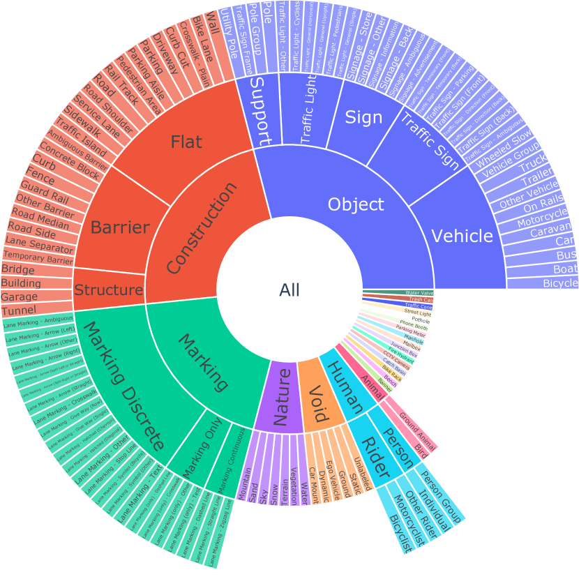
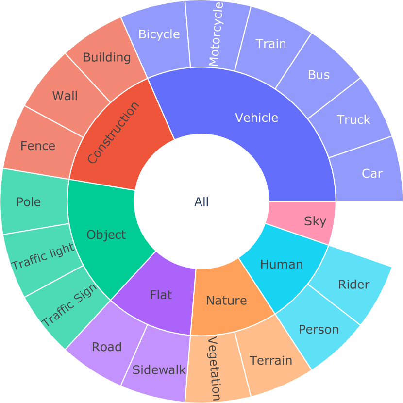
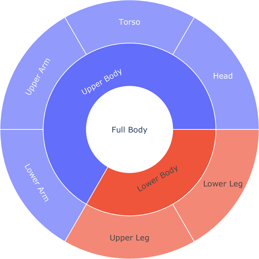
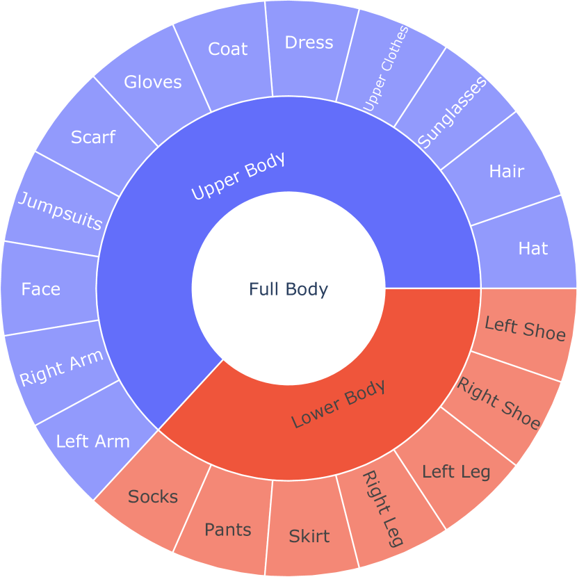
We use the official hierarchical structure provided in each dataset. Detailed semantic hierarchies are provided in Fig.${}_{\!}$ A.1 for Mapillary Vistas 2.0 [58], Fig.${}_{\!}$ A.2 for Cityscapes [18], Fig.${}_{\!}$ A.3 for PASCAL-Person-Part [87] and Fig.${}_{\!}$ A.4 for LIP [44]. For Mapillary Vistas 2.0 and Cityscapes, we add a virtual root node (i.e., All) to represent the most general concept.

$m_{\varepsilon}$ in Eq. 8	$\text{mIoU}^{2}$$\uparrow$	$\text{mIoU}^{1}$$\uparrow$
0.05	93.16 (-0.13)	82.81 (-0.18)
0.10 (default)	93.29	82.99
0.15	93.19 (-0.10)	82.86 (-0.13)

(a)

0.5 in Eq. 8	$\text{mIoU}^{2}$$\uparrow$	$\text{mIoU}^{1}$$\uparrow$
0.45	93.17 (-0.12)	82.84 (-0.15)
0.50 (default)	93.29	82.99
0.55	93.13 (-0.16)	82.80 (-0.19)

(b)

$\beta$ Schedule	Value	$\text{mIoU}^{2}$$\uparrow$	$\text{mIoU}^{1}$$\uparrow$
Cosine (default)	0 $\rightarrow$ 0.5	93.29	82.99
Constant	0.5	93.02 (-0.27)	82.68 (-0.31)

(c)

Table C.1: More ablative experiments for hyper-parameters​ (§C) on Cityscapes​ [18] val.

Appendix B Additional Qualitative Result

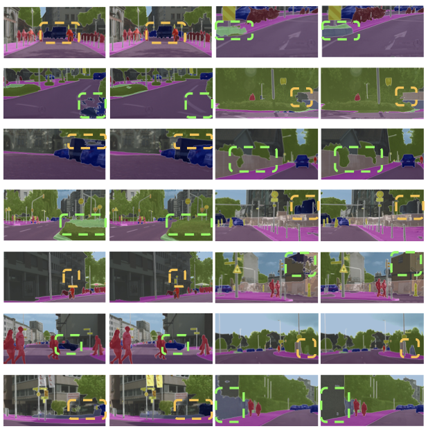
We provide additional visualization results on four datasets, including Mapillary Vistas 2.0 [58] val in Fig.${}_{\!}$ B.1, Cityscapes [18] val in Fig.${}_{\!}$ B.2, PASCAL-Person-Part [87] val in Fig.${}_{\!}$ B.3 and LIP [44] val in Fig.${}_{\!}$ B.4. The left column shows results from the baseline model while the right column is the predictions produced by Hssn. We see that Hssn yields consistently better visual effects than the baseline model.

Appendix C Additional Ablative Study

We give extra ablative studies for the hyper-parameters emerged in our approach in Table C.1. It can be seen that, for $m_{\varepsilon}$ and 0.5 in Eq. 8, there is minor impact to the perfromance. This indicates our method is robust to hyper-parameters. For the balance factor $\beta$ between $\mathcal{L}^{\text{FTM}}$ and $\mathcal{L}^{\text{TT}}$, scheduling it in a cosine annealing policy yields better performance. It is reasonable due to the poor recognition capability of the network at the initial stage of training.

Appendix D Discussion on Triplet Number

We further investigate the impact of the number of triplets in $\mathcal{L}^{\text{TT}}$ sampled druing training on performance. It can be seen in Table D.1 that the introduce of triplet loss imposes additional computation to the model and slows down the training speed. However, Hssn is able to reach very promising performance using a small number of triplets (e.g., 200) on both datasets. Further increasing the number only brings minor improvements. Based on the results in Table D.1, we set the number to 200 for all datasets. This facilitates Hssn to perform triplet sampling at negligible cost and be rewarded with impressive performance boost.

		Mapillary Vistas 2.0		PASCAL-Person-Part
#	# Triplets	mIoU$\uparrow$	Time $\downarrow$	mIoU $\uparrow$	Time $\downarrow$
1	–	39.17	0.93	72.89	0.41
2	100	39.82 (-0.34)	1.06 (-0.12)	74.76 (-0.68)	0.52 (-0.20)
3	200 (default)	40.16	1.18	75.44	0.58
4	500	40.19 (+0.03)	1.58 (+0.40)	75.53 (+0.09)	0.72 (+0.14)

Table D.1: Impact of pixel triplet number (§D) on Mapillary Vistas $2.0$ [58] val and PASCAL-Person-Part [87] test. Time indicates training time (second) for each batch.

Figure A.1: Hierarchical architecture of Mapillary Vistas 2.0​ [58].

Figure A.2: Hierarchical architecture of Cityscapes​ [18].

Figure A.3: Hierarchical architecture of PASCAL-Person-Part​ [87].

Figure A.4: Hierarchical architecture of LIP​ [44].

Figure B.1: More visualization results for semantic segmentation on Mapillary Vistas 2.0​ [58] val.

Figure B.2: More visualization results for semantic segmentation on Cityscapes​ [18] val.

Figure B.3: More visualization results for human parsing on PASCAL-Person-Part​ [87] val.

Figure B.4: More visualization results for human parsing on LIP​ [44] val.

References

- [1] Karim Ahmed, Mohammad Haris Baig, and Lorenzo Torresani. Network of experts for large-scale image categorization. In ECCV, 2016.
- [2] Zeynep Akata, Scott Reed, Daniel Walter, Honglak Lee, and Bernt Schiele. Evaluation of output embeddings for fine-grained image classification. In CVPR, 2015.
- [3] Vijay Badrinarayanan, Alex Kendall, and Roberto Cipolla. Segnet: A deep convolutional encoder-decoder architecture for image segmentation. IEEE TPAMI, 39(12):2481–2495, 2017.
- [4] Zafer Barutcuoglu, Robert E Schapire, and Olga G Troyanskaya. Hierarchical multi-label prediction of gene function. Bioinformatics, 22(7):830–836, 2006.
- [5] Björn Barz and Joachim Denzler. Hierarchy-based image embeddings for semantic image retrieval. In WACV, 2019.
- [6] Samy Bengio, Jason Weston, and David Grangier. Label embedding trees for large multi-class tasks. In NeurIPS, 2010.
- [7] Luca Bertinetto, Romain Mueller, Konstantinos Tertikas, Sina Samangooei, and Nicholas A Lord. Making better mistakes: Leveraging class hierarchies with deep networks. In CVPR, 2020.
- [8] Wei Bi and James T Kwok. Multilabel classification on tree-and dag-structured hierarchies. In ICML, 2011.
- [9] Alsallakh Bilal, Amin Jourabloo, Mao Ye, Xiaoming Liu, and Liu Ren. Do convolutional neural networks learn class hierarchy? TVCG, 2017.
- [10] Liang-Chieh Chen, George Papandreou, Iasonas Kokkinos, Kevin Murphy, and Alan L Yuille. Deeplab: Semantic image segmentation with deep convolutional nets, atrous convolution, and fully connected crfs. TPAMI, 2017.
- [11] Liang-Chieh Chen, George Papandreou, Florian Schroff, and Hartwig Adam. Rethinking atrous convolution for semantic image segmentation. arXiv preprint arXiv:1706.05587, 2017.
- [12] Liang-Chieh Chen, Yi Yang, Jiang Wang, Wei Xu, and Alan L Yuille. Attention to scale: Scale-aware semantic image segmentation. In CVPR, 2016.
- [13] Liang-Chieh Chen, Yukun Zhu, George Papandreou, Florian Schroff, and Hartwig Adam. Encoder-decoder with atrous separable convolution for semantic image segmentation. In ECCV, 2018.
- [14] Tianshui Chen, Wenxi Wu, Yuefang Gao, Le Dong, Xiaonan Luo, and Liang Lin. Fine-grained representation learning and recognition by exploiting hierarchical semantic embedding. In ACMMM, 2018.
- [15] Bowen Cheng, Liang-Chieh Chen, Yunchao Wei, Yukun Zhu, Zilong Huang, Jinjun Xiong, Thomas S Huang, Wen-Mei Hwu, and Honghui Shi. Spgnet: Semantic prediction guidance for scene parsing. In ICCV, 2019.
- [16] Bowen Cheng, Alexander G. Schwing, and Alexander Kirillov. Per-pixel classification is not all you need for semantic segmentation. In NeurIPS, 2021.
- [17] Sungha Choi, Joanne T Kim, and Jaegul Choo. Cars can’t fly up in the sky: Improving urban-scene segmentation via height-driven attention networks. In CVPR, 2020.
- [18] Marius Cordts, Mohamed Omran, Sebastian Ramos, Timo Rehfeld, Markus Enzweiler, Rodrigo Benenson, Uwe Franke, Stefan Roth, and Bernt Schiele. The cityscapes dataset for semantic urban scene understanding. In CVPR, 2016.
- [19] Jifeng Dai, Haozhi Qi, Yuwen Xiong, Yi Li, Guodong Zhang, Han Hu, and Yichen Wei. Deformable convolutional networks. In CVPR, 2017.
- [20] Ofer Dekel, Joseph Keshet, and Yoram Singer. Large margin hierarchical classification. In ICML, 2004.
- [21] Jia Deng, Alexander C Berg, Kai Li, and Li Fei-Fei. What does classifying more than 10,000 image categories tell us? In ECCV, 2010.
- [22] Jia Deng, Wei Dong, Richard Socher, Li-Jia Li, Kai Li, and Li Fei-Fei. Imagenet: A large-scale hierarchical image database. In CVPR, 2009.
- [23] Henghui Ding, Xudong Jiang, Ai Qun Liu, Nadia Magnenat Thalmann, and Gang Wang. Boundary-aware feature propagation for scene segmentation. In CVPR, 2019.
- [24] Andrea Frome, Greg S Corrado, Jonathon Shlens, Samy Bengio, Jeffrey Dean, Marc’Aurelio Ranzato, and Tomas Mikolov. Devise: a deep visual-semantic embedding model. In NeurIPS, 2013.
- [25] Jun Fu, Jing Liu, Haijie Tian, Yong Li, Yongjun Bao, Zhiwei Fang, and Hanqing Lu. Dual attention network for scene segmentation. In CVPR, 2019.
- [26] Octavian Ganea, Gary Bécigneul, and Thomas Hofmann. Hyperbolic entailment cones for learning hierarchical embeddings. In ICML, 2018.
- [27] Vivien Sainte Fare Garnot and Loic Landrieu. Leveraging class hierarchies with metric-guided prototype learning. arXiv preprint arXiv:2007.03047, 2020.
- [28] Weifeng Ge. Deep metric learning with hierarchical triplet loss. In ECCV, 2018.
- [29] Eleonora Giunchiglia and Thomas Lukasiewicz. Coherent hierarchical multi-label classification networks. NeurIPS, 2020.
- [30] Ke Gong, Yiming Gao, Xiaodan Liang, Xiaohui Shen, Meng Wang, and Liang Lin. Graphonomy: Universal human parsing via graph transfer learning. In CVPR, 2019.
- [31] Feng Han and Song-Chun Zhu. Bottom-up/top-down image parsing with attribute grammar. PAMI, 31(1):59–73, 2008.
- [32] Adam W Harley, Konstantinos G Derpanis, and Iasonas Kokkinos. Segmentation-aware convolutional networks using local attention masks. In ICCV, 2017.
- [33] Junjun He, Zhongying Deng, Lei Zhou, Yali Wang, and Yu Qiao. Adaptive pyramid context network for semantic segmentation. In CVPR, 2019.
- [34] Kaiming He, Xiangyu Zhang, Shaoqing Ren, and Jian Sun. Deep residual learning for image recognition. In CVPR, 2016.
- [35] Zilong Huang, Xinggang Wang, Lichao Huang, Chang Huang, Yunchao Wei, and Wenyu Liu. Ccnet: Criss-cross attention for semantic segmentation. In ICCV, 2019.
- [36] Ruyi Ji, Dawei Du, Libo Zhang, Longyin Wen, Yanjun Wu, Chen Zhao, Feiyue Huang, and Siwei Lyu. Learning semantic neural tree for human parsing. In ECCV, 2020.
- [37] Daniel Kaiser, Genevieve L Quek, Radoslaw M Cichy, and Marius V Peelen. Object vision in a structured world. Trends in cognitive sciences, 23(8):672–685, 2019.
- [38] Tommi Kerola, Jie Li, Atsushi Kanehira, Yasunori Kudo, Alexis Vallet, and Adrien Gaidon. Hierarchical lovász embeddings for proposal-free panoptic segmentation. In CVPR, 2021.
- [39] Daphne Koller and Mehran Sahami. Hierarchically classifying documents using very few words. In ICML, 1997.
- [40] Hanchao Li, Pengfei Xiong, Jie An, and Lingxue Wang. Pyramid attention network for semantic segmentation. arXiv preprint arXiv:1805.10180, 2018.
- [41] Xiangtai Li, Xia Li, Li Zhang, Guangliang Cheng, Jianping Shi, Zhouchen Lin, Shaohua Tan, and Yunhai Tong. Improving semantic segmentation via decoupled body and edge supervision. In ECCV, 2020.
- [42] Xia Li, Zhisheng Zhong, Jianlong Wu, Yibo Yang, Zhouchen Lin, and Hong Liu. Expectation-maximization attention networks for semantic segmentation. In ICCV, 2019.
- [43] Zhiheng Li, Wenxuan Bao, Jiayang Zheng, and Chenliang Xu. Deep grouping model for unified perceptual parsing. In CVPR, 2020.
- [44] Xiaodan Liang, Ke Gong, Xiaohui Shen, and Liang Lin. Look into person: Joint body parsing & pose estimation network and a new benchmark. TPAMI, 2018.
- [45] Xiaodan Liang, Hongfei Zhou, and Eric Xing. Dynamic-structured semantic propagation network. In CVPR, 2018.
- [46] Guosheng Lin, Anton Milan, Chunhua Shen, and Ian Reid. Refinenet: Multi-path refinement networks for high-resolution semantic segmentation. In CVPR, 2017.
- [47] Tsung-Yi Lin, Priya Goyal, Ross Girshick, Kaiming He, and Piotr Dollár. Focal loss for dense object detection. In ICCV, 2017.
- [48] Xinchen Liu, Meng Zhang, Wu Liu, Jingkuan Song, and Tao Mei. Braidnet: Braiding semantics and details for accurate human parsing. In ACM MM, 2019.
- [49] Ze Liu, Yutong Lin, Yue Cao, Han Hu, Yixuan Wei, Zheng Zhang, Stephen Lin, and Baining Guo. Swin transformer: Hierarchical vision transformer using shifted windows. ICCV, 2021.
- [50] Jonathan Long, Evan Shelhamer, and Trevor Darrell. Fully convolutional networks for semantic segmentation. In CVPR, 2015.
- [51] Ilya Loshchilov and Frank Hutter. Sgdr: Stochastic gradient descent with warm restarts. In ICLR, 2017.
- [52] Ilya Loshchilov and Frank Hutter. Decoupled weight decay regularization. ICLR, 2019.
- [53] Xiankai Lu, Wenguan Wang, Jianbing Shen, David Crandall, and Luc Van Gool. Segmenting objects from relational visual data. IEEE TPAMI, 2021.
- [54] Yawei Luo, Zhedong Zheng, Liang Zheng, Tao Guan, Junqing Yu, and Yi Yang. Macro-micro adversarial network for human parsing. In ECCV, 2018.
- [55] Andrew McCallum, Ronald Rosenfeldy, Tom Mitchelly, and Andrew Y Ngz. Improving text classification by shrinkage in a hierarchy of classes. In ICML, 1998.
- [56] Panagiotis Meletis and Gijs Dubbelman. Training of convolutional networks on multiple heterogeneous datasets for street scene semantic segmentation. In IEEE Intelligent Vehicles Symposium, 2018.
- [57] Seyedeh Fatemeh Mousavi, Mehran Safayani, Abdolreza Mirzaei, and Hoda Bahonar. Hierarchical graph embedding in vector space by graph pyramid. PR, 2017.
- [58] Gerhard Neuhold, Tobias Ollmann, Samuel Rota Bulo, and Peter Kontschieder. The mapillary vistas dataset for semantic understanding of street scenes. In ICCV, 2017.
- [59] Maximillian Nickel and Douwe Kiela. Poincaré embeddings for learning hierarchical representations. NeurIPS, 2017.
- [60] Zhenxing Niu, Mo Zhou, Le Wang, Xinbo Gao, and Gang Hua. Hierarchical multimodal lstm for dense visual-semantic embedding. In ICCV, 2017.
- [61] Lorenzo Porzi, Samuel Rota Bulo, Aleksander Colovic, and Peter Kontschieder. Seamless scene segmentation. In CVPR, 2019.
- [62] Olaf Ronneberger, Philipp Fischer, and Thomas Brox. U-net: Convolutional networks for biomedical image segmentation. In MICCAI, 2015.
- [63] Juho Rousu, Craig Saunders, Sandor Szedmak, and John Shawe-Taylor. Kernel-based learning of hierarchical multilabel classification models. Journal of Machine Learning Research, 7:1601–1626, 2006.
- [64] Tao Ruan, Ting Liu, Zilong Huang, Yunchao Wei, Shikui Wei, and Yao Zhao. Devil in the details: Towards accurate single and multiple human parsing. In AAAI, 2019.
- [65] Frederic Sala, Chris De Sa, Albert Gu, and Christopher Ré. Representation tradeoffs for hyperbolic embeddings. In ICML, 2018.
- [66] Florian Schroff, Dmitry Kalenichenko, and James Philbin. Facenet: A unified embedding for face recognition and clustering. In CVPR, 2015.
- [67] Carlos N Silla and Alex A Freitas. A survey of hierarchical classification across different application domains. Data Mining and Knowledge Discovery, 22(1):31–72, 2011.
- [68] Elizabeth S Spelke and Katherine D Kinzler. Core knowledge. Developmental science, 10(1):89–96, 2007.
- [69] Robin Strudel, Ricardo Garcia, Ivan Laptev, and Cordelia Schmid. Segmenter: Transformer for semantic segmentation. In ICCV, 2021.
- [70] Erik B Sudderth, Antonio Torralba, William T Freeman, and Alan S Willsky. Learning hierarchical models of scenes, objects, and parts. In ICCV, 2005.
- [71] Erik B Sudderth, Antonio Torralba, William T Freeman, and Alan S Willsky. Describing visual scenes using transformed objects and parts. IJCV, 77(1-3):291–330, 2008.
- [72] Aixin Sun and Ee-Peng Lim. Hierarchical text classification and evaluation. In International Conference on Data Mining, 2001.
- [73] Guolei Sun, Wenguan Wang, Jifeng Dai, and Luc Van Gool. Mining cross-image semantics for weakly supervised semantic segmentation. In ECCV, 2020.
- [74] Zhuowen Tu, Xiangrong Chen, Alan L Yuille, and Song-Chun Zhu. Image parsing: Unifying segmentation, detection, and recognition. IJCV, 63(2):113–140, 2005.
- [75] Giorgio Valentini. True path rule hierarchical ensembles for genome-wide gene function prediction. IEEE/ACM Transactions on Computational Biology and Bioinformatics, 8(3):832–847, 2010.
- [76] Ashish Vaswani, Noam Shazeer, Niki Parmar, Jakob Uszkoreit, Llion Jones, Aidan N Gomez, Lukasz Kaiser, and Illia Polosukhin. Attention is all you need. In NeurIPS, 2017.
- [77] Ivan Vendrov, Ryan Kiros, Sanja Fidler, and Raquel Urtasun. Order-embeddings of images and language. In ICLR, 2016.
- [78] Nakul Verma, Dhruv Mahajan, Sundararajan Sellamanickam, and Vinod Nair. Learning hierarchical similarity metrics. In CVPR, 2012.
- [79] Jingdong Wang, Ke Sun, Tianheng Cheng, Borui Jiang, Chaorui Deng, Yang Zhao, Dong Liu, Yadong Mu, Mingkui Tan, Xinggang Wang, et al. Deep high-resolution representation learning for visual recognition. TPAMI, 2020.
- [80] Wenguan Wang, Zhijie Zhang, Siyuan Qi, Jianbing Shen, Yanwei Pang, and Ling Shao. Learning compositional neural information fusion for human parsing. In ICCV, 2019.
- [81] Wenguan Wang, Tianfei Zhou, Siyuan Qi, Jianbing Shen, and Song-Chun Zhu. Hierarchical human semantic parsing with comprehensive part-relation modeling. IEEE TPAMI, 2021.
- [82] Wenguan Wang, Tianfei Zhou, Fisher Yu, Jifeng Dai, Ender Konukoglu, and Luc Van Gool. Exploring cross-image pixel contrast for semantic segmentation. In ICCV, 2021.
- [83] Wenguan Wang, Hailong Zhu, Jifeng Dai, Yanwei Pang, Jianbing Shen, and Ling Shao. Hierarchical human parsing with typed part-relation reasoning. In CVPR, 2020.
- [84] Xiaolong Wang, Ross Girshick, Abhinav Gupta, and Kaiming He. Non-local neural networks. In CVPR, 2018.
- [85] Jonatas Wehrmann, Ricardo Cerri, and Rodrigo Barros. Hierarchical multi-label classification networks. In ICML, 2018.
- [86] Kilian Q Weinberger and Olivier Chapelle. Large margin taxonomy embedding for document categorization. In NeurIPS, 2009.
- [87] Fangting Xia, Peng Wang, Xianjie Chen, and Alan L Yuille. Joint multi-person pose estimation and semantic part segmentation. In CVPR, 2017.
- [88] Yongqin Xian, Zeynep Akata, Gaurav Sharma, Quynh Nguyen, Matthias Hein, and Bernt Schiele. Latent embeddings for zero-shot classification. In CVPR, 2016.
- [89] Tete Xiao, Yingcheng Liu, Bolei Zhou, Yuning Jiang, and Jian Sun. Unified perceptual parsing for scene understanding. In ECCV, 2018.
- [90] Enze Xie, Wenhai Wang, Zhiding Yu, Anima Anandkumar, Jose M Alvarez, and Ping Luo. Segformer: Simple and efficient design for semantic segmentation with transformers. In NeurIPS, 2021.
- [91] Zhicheng Yan, Hao Zhang, Robinson Piramuthu, Vignesh Jagadeesh, Dennis DeCoste, Wei Di, and Yizhou Yu. Hd-cnn: hierarchical deep convolutional neural networks for large scale visual recognition. In ICCV, 2015.
- [92] Jie Yang, Jiarou Fan, Yiru Wang, Yige Wang, Weihao Gan, Lin Liu, and Wei Wu. Hierarchical feature embedding for attribute recognition. In CVPR, 2020.
- [93] Maoke Yang, Kun Yu, Chi Zhang, Zhiwei Li, and Kuiyuan Yang. Denseaspp for semantic segmentation in street scenes. In CVPR, 2018.
- [94] Shuo Yang, Wei Yu, Ying Zheng, Hongxun Yao, and Tao Mei. Adaptive semantic-visual tree for hierarchical embeddings. In ACMMM, 2019.
- [95] Yi Yang, Yueting Zhuang, and Yunhe Pan. Multiple knowledge representation for big data artificial intelligence: framework, applications, and case studies. Frontiers of Information Technology & Electronic Engineering, 22(12):1551–1558, 2021.
- [96] Jian Yao, Sanja Fidler, and Raquel Urtasun. Describing the scene as a whole: Joint object detection, scene classification and semantic segmentation. In CVPR, 2012.
- [97] Fisher Yu and Vladlen Koltun. Multi-scale context aggregation by dilated convolutions. In ICLR, 2016.
- [98] Yuhui Yuan, Xilin Chen, and Jingdong Wang. Object-contextual representations for semantic segmentation. In ECCV, 2020.
- [99] Yuhui Yuan, Jingyi Xie, Xilin Chen, and Jingdong Wang. Segfix: Model-agnostic boundary refinement for segmentation. In ECCV, 2020.
- [100] Fan Zhang, Yanqin Chen, Zhihang Li, Zhibin Hong, Jingtuo Liu, Feifei Ma, Junyu Han, and Errui Ding. Acfnet: Attentional class feature network for semantic segmentation. In ICCV, 2019.
- [101] Xiaomei Zhang, Yingying Chen, Bingke Zhu, Jinqiao Wang, and Ming Tang. Part-aware context network for human parsing. In CVPR.
- [102] Xiaomei Zhang, Yingying Chen, Bingke Zhu, Jinqiao Wang, and Ming Tang. Blended grammar network for human parsing. In ECCV, 2020.
- [103] Bin Zhao, Li Fei-Fei, and Eric P Xing. Large-scale category structure aware image categorization. In NeurIPS, 2011.
- [104] Hang Zhao, Xavier Puig, Bolei Zhou, Sanja Fidler, and Antonio Torralba. Open vocabulary scene parsing. In ICCV, 2017.
- [105] Hengshuang Zhao, Jianping Shi, Xiaojuan Qi, Xiaogang Wang, and Jiaya Jia. Pyramid scene parsing network. In CVPR, 2017.
- [106] Hengshuang Zhao, Yi Zhang, Shu Liu, Jianping Shi, Chen Change Loy, Dahua Lin, and Jiaya Jia. Psanet: Point-wise spatial attention network for scene parsing. In ECCV, 2018.
- [107] Sixiao Zheng, Jiachen Lu, Hengshuang Zhao, Xiatian Zhu, Zekun Luo, Yabiao Wang, Yanwei Fu, Jianfeng Feng, Tao Xiang, Philip HS Torr, et al. Rethinking semantic segmentation from a sequence-to-sequence perspective with transformers. In CVPR, 2021.
- [108] Tianfei Zhou, Liulei Li, Xueyi Li, Chun-Mei Feng, Jianwu Li, and Ling Shao. Group-wise learning for weakly supervised semantic segmentation. IEEE TIP, 31:799–811, 2021.
- [109] Tianfei Zhou, Siyuan Qi, Wenguan Wang, Jianbing Shen, and Song-Chun Zhu. Cascaded parsing of human-object interaction recognition. IEEE TPAMI, 2021.
- [110] Tianfei Zhou, Wenguan Wang, Si Liu, Yi Yang, and Luc Van Gool. Differentiable multi-granularity human representation learning for instance-aware human semantic parsing. In CVPR, 2021.
- [111] Bingke Zhu, Yingying Chen, Ming Tang, and Jinqiao Wang. Progressive cognitive human parsing. In AAAI, 2018.
- [112] Xinqi Zhu and Michael Bain. B-cnn: branch convolutional neural network for hierarchical classification. arXiv preprint arXiv:1709.09890, 2017.
- [113] Zhen Zhu, Mengde Xu, Song Bai, Tengteng Huang, and Xiang Bai. Asymmetric non-local neural networks for semantic segmentation. In ICCV, 2019.
- [114] Alon Zweig and Daphna Weinshall. Exploiting object hierarchy: Combining models from different category levels. In ICCV, 2007.