Safe Hierarchical Model Predictive Control and Planning for Autonomous Systems

Abstract

[Abstract]Planning and control for autonomous vehicles usually are hierarchical separated. However, increasing performance demands and operating in highly dynamic environments requires an frequent re-evaluation of the planning and tight integration of control and planning to guarantee safety. We propose an integrated hierarchical predictive control and planning approach to tackle this challenge. Planner and controller are based on the repeated solution of moving horizon optimal control problems. The planner can choose different low-layer controller modes for increased flexibility and performance instead of using a single controller with a large safety margin for collision avoidance under uncertainty. Planning is based on simplified system dynamics and safety, yet flexible operation is ensured by constraint tightening based on a mixed-integer linear programming formulation. A cyclic horizon tube-based model predictive controller guarantees constraint satisfaction for different control modes and disturbances. Examples of such modes are a slow-speed movement with high precision and fast-speed movements with large uncertainty bounds. Allowing for different control modes reduces the conservatism, while the hierarchical decomposition of the problem reduces the computational cost and enables real-time implementation. We derive conditions for recursive feasibility to ensure constraint satisfaction and obstacle avoidance to guarantee safety and ensure compatibility between the layers and modes. Simulation results illustrate the efficiency and applicability of the proposed hierarchical strategy.

1 Introduction

Autonomous vehicles, such as drones, mobile robots, or autonomous transportation systems, are by now used in a wide range of applications, spanning from geo-surveillance, agricultural application, logistics, or search and rescue operations ^{1, 2}. Often, the autonomous vehicle has to achieve a task, like to move from a start to a goal position, while avoiding obstacles in a dynamically changing environment, compare Figure 1.

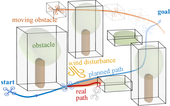
Figure 1: Planning and control for autonomous vehicles in uncertain, dynamically changing environments, e.g., moving obstacles or wind, with collision avoidance.

Safe operation, i.e., collision avoidance, under all circumstances is challenging ^{3, 4, 5}. Typically, the task is hierarchically separated into a planning task performed once or repeatedly on a slow time scale. It provides a reference or path to a lower-layer control layer that operates on a fast time scale to counteract disturbances, model uncertainty, or react to (fast) environmental changes, c.f. Figure 2 (a), see also.  ^{6, 7, 8, 9, 10, 11, 12, 13}

Many planning approaches for autonomous vehicles exist, see, e.g., ^{1, 14, 15, 16} and references their-in. They, for example, exploit deterministic or heuristic search strategies, or reformulate the problem as a mathematical optimization problem. However, most of them do not allow considering detailed vehicle dynamics, environmental conditions, or disturbances explicitly.

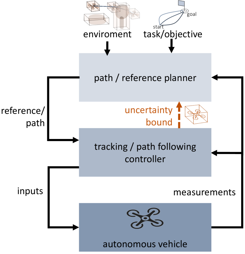
((a)) Typical decomposition of planning and control.

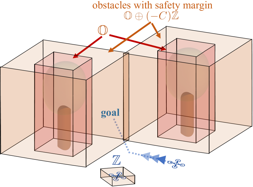
((b)) Safe planning by constraint tightening/constraint back off considering a single, fixed tracking control mode.

Figure 2: (a) Hierarchical separation of the planning and control layers; (b) Safe planning with a single tracking control mode.

Counteracting significant uncertainties, e.g., due to changing environmental conditions like wind, or operating in a dynamically evolving environment, requires frequent replanning and tightly integrating control and planning. This has attracted significant research over the past years: A multi-rate hierarchical approach consisting of three control layers operating at different sampling times is presented in ⁶. A Markov decision problem is exploited on the highest planning layer, which feeds into the planning/reference generation layer, exploiting a model predictive control formulation. At the lowest layer, a tracking controller is considered that uses a barrier function approach. In ⁷ an approach to co-design the planner and control is proposed, which allows considering vehicle dynamics and kinematic constraints. The tracking error of the controller is directly considered in the planner. A multi-layer control framework was presented in ¹⁰, where the optimization-based reference planner used a low fidelity model. At the same time, a feedback controller tracks the planned trajectory with a specific error bound. The state and input constraints are taken into account in the planning layer. The tracking control law and its error bounds are parameterized and computed offline using sum-of-squares programming. The approach allows maintaining safety by taking the tracking error bound into account to achieve maximum permissiveness of the planning layer. A two-layer model predictive control framework is presented in ¹², where the upper-layer controller determines the state trajectories over the entire mission while guaranteeing the satisfaction of the system constraint during operation. The lower-layer controller modifies the determined trajectories to improve reference tracking. In ¹³, a stable hierarchical model predictive control (MPC) is introduced using an inner loop reference model and contracting constraint sets for guaranteeing the overall stability. The inner-loop controller tracks the output of a prescribed reference model.

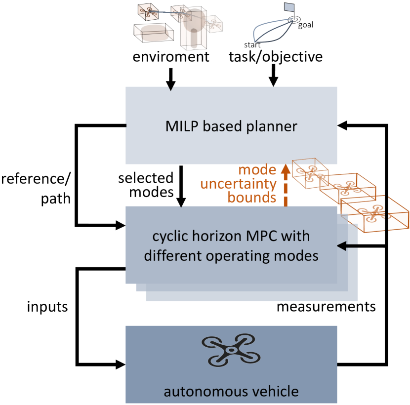
((a)) Proposed moving horizon planning and control exploiting multiple controller operation regions/modes.

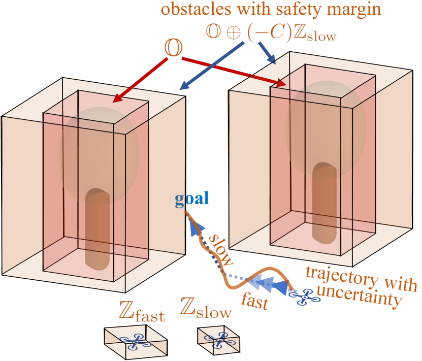
((b)) Reduced conservatism due to different tracking controller operation regions/modes.

Figure 3: Proposed planning and control scheme with multiple tracking controller operation regions/modes.

We propose a tightly integrated hierarchical planning and control approach to reduce conservatism while being computational feasible. Both planner and controller are based on the repeated solution of moving horizon optimal control problems. In particular, both layers are based on robust MPC ^{17, 18, 19, 20, 21} formulations. The planning- and the lower-layer controller agree on “contracts” (safety corridors), guaranteeing consistency and compatibility between the layers. Consequently, this ensures robust satisfaction of the constraints such as collision avoidance even in the presence of disturbances. The planner can choose different operating modes, corresponding to different accuracy’s that the lower-layer controller can achieve in the closed-loop. In comparison, existing hierarchical formulations often rely on a single yet conservative tracking controller mode, c.f., Fig 2.

A specific example of such modes is a slow-speed movement with high precision and a fast-speed movement with large uncertainty bounds, c.f., 3(b). As illustrated in Fig. 3(a) (b), the two control modes enable the planner to provide a collision-free path by switching online between different velocity ranges and corresponding controller parametrization.

We propose a moving horizon formulation for the planning layer, resulting in an efficiently solvable mixed-integer linear programming (MILP). The tracking control for the vehicle is achieved by a cyclic horizon MPC ^{20, 22}, which operates with a high sampling frequency. The tracking controller provides safety bounds for each operation mode, despite disturbances. We derive conditions for recursive feasibility to ensure constraint satisfaction and obstacle avoidance. Simulation results illustrate the efficiency and applicability of the proposed hierarchical strategy. Especially, it is shown how different modes reduce the conservatism, while the decomposition of the control problem limits the computational cost and enables real-time implementation while providing guarantees.

The presented results are based on the results presented in ²³. They are expanded with respect to less conservative conditions and formulations and the overall approach is evaluated considering a quadcopter operating in a 3D environment.

The main contributions of this work are threefold:

1. First, we outline a planning approach operating on a moving horizon, which allows us to consider different tracking controller modes. We show how this approach can be reformulated as a MILP, which can be efficiently solved in real-time.

2. Second, we design a low-layer cyclic horizon tube MPC controller, which provides safety bounds, i.e., tubes, for the different modes, e.g., velocities. This controller guarantees in combination with the planning layer constraint satisfaction and collision avoidance.

3. Finally, we demonstrate our approach, considering a quadcopter operating in a 3D environment.

The remainder of the paper is organized as follows. Section 2 presents the problem setup. Section 3 outlines the hierarchy planning and control scheme, where Section 3.1 presents the MILP moving horizon planning problem. Section 3.2 describes the low-layer cyclic horizon tube MPC and Section 3.3 outlines the switching between the operating modes. Section 4 presents the simulation example and results for an quadcopter, while Section 5 recapitulates our findings, conclusions, and outlooks.

Notation For two given sets $\mathbb{X},\mathbb{Y}\subset\mathbb{R}^{n}$, the Minkowski set sum $\oplus$ and the Minkowski set difference $\ominus$ are defined by: $\mathbb{X}\oplus\mathbb{Y}\triangleq\{x+y|x\in\mathbb{X},y\in\mathbb{Y}\}$, $\mathbb{X}\ominus\mathbb{Y}\triangleq\{x|x\oplus\mathbb{Y}\subseteq\mathbb{X}$. We use $\operatorname{rem}$ to denote the remainder function of Euclidean division, $\mathbf{1}$ denotes a column vector with $1$ in each entry, and $\|x\|_{Q}^{2}=x^{T}Qx$.

2 Problem Formulation

We consider the control of an autonomous vehicle, which should move (drive, fly, etc.) from a starting point, $x(0)$, to a goal, $x_{\text{goal}}$, while avoiding obstacles and satisfying constraints despite uncertainties and disturbances, see Fig. 1. We assume that the vehicle dynamics are subject to unknown but bounded additive disturbances and that they are governed by

$$x(k+1)=\, Ax(k)+Bu(k)+w(k),$$ (1a)

$$y(k)=\, Cx(k),$$ (1b)

$$x(k)\in\, \mathbb{X},\,\,u(k)\in\mathbb{U}.$$ (1c)

Here $x(k)\in\mathbb{R}^{n}$ is the vehicle’s state, $u(k)\in\mathbb{R}^{m}$ is the applied control input, and the output $y(k)\in\mathbb{R}^{p}$, while $w(k)$ is an unknown, but bounded disturbance. The state $x(k)$ and the input $u(k)$ need to satisfy constraints: they are restricted to the sets $\mathbb{X}$ and $\mathbb{U}$, which are both closed and convex.

Obstacle avoidance: Beside the constraints (1c) on the state $x(k)$ and input $u(k)$ of the autonomous vehicle, we want to achieve obstacle avoidance, which we formulate in terms of the output $y(k)$ (e.g. the position). We assume that there are $H$ obstacles and that each obstacle is modeled as a bounded set of the form $\mathbb{O}_{\ell}=\{y|E_{\ell}y<f_{\ell}\}$, where $E_{\ell}\in\mathbb{R}^{q_{\ell}\times p}$. So, $\mathbb{O}_{\ell}$ is the interior of a convex, compact polytope. In the most simple case (box obstacles) $E_{\ell}=[I\,\,-I]$. Consequently, to avoid that the vehicle collides or touches the obstacles we require that:

$$y(k)\notin\mathbb{O},\,\,\mathbb{O}=\{E_{\ell}y(k)<f_{\ell},\,\,l=1,\ldots,H\},$$ (2)

where $\mathbb{O}$ is the collection of all $H$ obstacles. Clearly, the set of admissible output/position $y(k)\notin\mathbb{O}$, defined in (2), is non-convex, but contains its boundaries. One can also formulate it as

$$\forall\ell\in\{1,\ldots,H\},\,\,\exists a\in\{1,...,q_{\ell}\}:\ E_{\ell,a}y(k)\geq f_{\ell,a}.$$ (3)

This formulation allows to use a MILP framework with the so-called big-M approach, which enables handling the obstacles systematically, see Section 3.3.

Disturbance bounds and operating regions/modes: The disturbance $w(k)$, and its bounds, may depend in parts also on the vehicle’s state $x(k)$ and/or the applied control input $u(k)$. This might, for example be due to model uncertainties, which are captured as disturbances. For example, if the vehicle is operated at a lower speed, then the (worst case) disturbance might be smaller then at high speed.

Specifically, we consider discrete sets of disturbance bounds for different low-layer/tracking controllers operating modes, i.e., we assume that there are $N_{w}$ low-layer controller operating modes: (Operating region/mode dependent disturbance bounds)   There are $N_{w}$ low-layer controller operating regions/modes defined by the state and input sets $U_{i}$ and $X_{i}$ such that if $x(k)\in\mathbb{X}_{i}\subseteq\mathbb{X}$ and $u(k)\in\mathbb{U}_{i}\subseteq\mathbb{U}$, the uncertainty can be bounded by $w(k)\in\mathbb{W}_{i}$, where the sets $\mathbb{X}_{i}$, $\mathbb{U}_{i}$ are convex and closed polytopes and $\mathbb{W}_{i}$ is a convex and compact polytope. Note that the sets $\mathbb{X}_{i}$ (and $\mathbb{U}_{i}$) may overlap, i.e. one can have that $\mathbb{X}_{i}\cap\mathbb{X}_{j}\neq\emptyset$ for $i\neq j$.

3 Robust Hierarchical Moving Horizon Planning and Control

We focus on a hierarchical two-layer planning and control decomposition as depicted in Fig. 3(a), to achieve safe and collision-free motion of the autonomous vehicle to the goal. Both layers utilize (robust) MPC formulations for constraint satisfaction under uncertainties.

To provide guarantees despite the hierarchical decomposition of the problem in a planning and control layer, we utilize the concept of “contracts”, inspired by ^{24, 25, 26}. Loosely speaking, a contract specifies the achievable precision in terms of a bound on the disturbance the lower-layer tracking controller can achieve for a specific operating region/mode $i$ - a particular set of states and inputs. In the proposed approach, the moving horizon planner provides a reference path and selects the operating region the controller should operate in. To calculate a safe passage - satisfy the constraints (1c) and to avoid all obstacles (3) - the planner takes the uncertainty bounds corresponding to the different operating regions directly into account.

In detail the upper-layer planner calculates the reference based on a model with simplified dynamics of the form

$$x_{p}(k_{p}+1)=A_{p}x_{p}(k_{p})+B_{p}u_{p}(k_{p}),$$ (4)

where $k_{p}$ is the planning time index. The generated reference path and measurements of the vehicle’s state are used by the lower-layer controller to calculate the control input $u(k)$, see Fig. 2. The lower-layer control loop aims to efficiently counteract the disturbances, to ensure that the vehicle follows the planned reference with a specified accuracy, to satisfy the contract, and to guarantee constraint satisfaction. As the obstacles are handled by the planner, the tracking controller does not need to consider them, which enables a fast and efficient implementation as non-convex constraints are avoided.

We consider that the planning is done slowly, all $M\ (>1)$ time steps. So we have

$$k=k_{p}\cdot M,\quad A_{p}=A^{M},\quad B_{p}=\sum_{i=0}^{M-1}A^{i}B.$$ (5)

We assume that the the real dynamics (1a) and the "planning dynamics" (4) satisfy: (Controllability of the planning and control dynamics) The pairs $(A,B)$ and $(A_{p},B_{p})$ are controllable. Note that if $(A_{p},B_{p})$ is controllable, then also $(A,B)$. In principle, $(A_{p},B_{p})$ could be uncontrollable even if $(A,B)$ is controllable, see ²⁷.

The contracts ensure the planner that the lower-layer controller can bound the tracking error by

$$x\big{(}(k_{p}+1)\cdot M\big{)}-x_{p}(k_{p}+1)\in\mathbb{Z}_{i},$$ (6)

for $i=1,\ldots,N_{w}$, where the sets $\mathbb{Z}_{i}$ are convex, compact polytopes and $N_{w}$ is the number of the operating mode.

The lower-layer controller can guarantee the constraints, if $x\in\mathbb{X}_{i}$ and $u\in\mathbb{U}_{i}$, i.e., that the state and the input are inside the operation region $i$, see Assumption 2. Additionally, constraints due to the obstacle avoidance requirements and the different sampling times need to be satisfied, which are introduced in s second step. We assume that the contracts - the operating regions/modes - are designed offline and known by both control layers. They depend on the design of of the low-layer controller and the operation mode $i$, i.e., the (partly) selectable uncertainty bound $\mathbb{W}_{i}$ on the disturbance $w$. Summarizing: Utilizing the idea of contracts - different operating modes - enables the planner to utilize and take the capability of the low-layer control loop into account for the computation of the reference. Consequently, the planner calculates and sends to the low-layer controller a reference and selects via the choice of $\mathbb{Z}_{i}$ the maximum allowed tracking discrepancy. In other words, the reference planner can switch between different operation modes, in order to improve the performance, as illustrated in Fig. 3(b).

3.1 Upper-layer: Moving Horizon Reference Planning

The reference planer should guarantee constraint satisfaction, including obstacle avoidance, despite the presence of disturbances and uncertainties in combination with a suitably designed lower-layer control loop, compare Fig. 3(a).

The key idea is to incorporate the concept of contracts - different operating modes - into mathematical programming based moving horizon planning schemes^{28, 9, 29, 30, 31}. To do so, the reference planning problem $\mathcal{P}\big{(}x(k_{p}M)\big{)}$ is formulated on a moving horizon as a optimization problem:

$$\min_{\{x_{p}\},\{u_{p}\},i}J_{p}\big{(}\{x_{p}\},\{u_{p}\}\big{)}$$ , (7a)

s.t.

$$i \in\{1,\ldots,N_{w}\}$$ (7b)

$$x(k_{p}M)-x_{p}(k_{p}|k_{p}) \in\mathbb{Z}_{i},$$ (7c)

$$\forall j \in\{0,\ldots,N-1\}: x_{p}(k_{p}+j+1|k_{p}) =A_{p}x_{p}(k_{p}+j|k_{p})+B_{p}u_{p}(k_{p}+j|k_{p}),$$ (7d)

$$\forall j \in\{0,\ldots,N-1\}: x_{p}(k_{p}+j|k_{p}) \in\mathbb{X}_{i}\ominus\mathbb{Z}_{i},$$ (7e)

$$\forall j \in\{0,\ldots,N-1\}: u_{p}(k_{p}+j|k_{p}) \in\mathbb{U}_{i}\ominus{K}\mathbb{Z}_{i},$$ (7f)

$$\forall j \in\{0,\ldots,N-1\}: Cx_{p}(k_{p}+j|k_{p}) \notin\mathbb{O}\oplus(-C)\mathbb{Z}_{i},$$ (7g)

$$\forall j \in\{0,\ldots,N-1\}: \big{(}x_{p}(k_{p}+j|k_{p}),u_{p}(k_{p}+j|k_{p})\big{)} \in\mathbb{I}_{i},$$ (7h)

$$x_{p}(k_{p}+N|k_{p}) \in\mathbb{X}_{i}^{f}.$$ (7i)

Here $N$ denotes the planning horizon, $i$ the operation mode, and $(k_{p}+j|k_{p})$ corresponds to the prediction of a value at time $k_{p}+j$ made at time $k_{p}$. The constraint (7c) represent an initial constraint at the begin of the planning time $k_{p}$. Eq. (7d) represent the vehicle dynamics used by the planning layer. While the constraints (7e,7f) are the tightened state and input constraints, where $K$ is a control gain, which is discussed later in detail. For the output constraints (7g) the constraint tightening corresponds to an enlargement of the obstacles, see Fig. 3(b).

To allow for an efficient reformulation of (7) as an MILP, c.f. Section 3.3, we consider the following cost function

$$J_{\text{p}}\big{(}\{x_{p}\},\{u_{p}\}\big{)}=\|x_{\text{\tiny goal}}-x_{p}(k_{p}+N)\|_{\infty}+\sum_{j=k_{p}}^{k_{p}+N-1}\alpha_{x}\|{x}_{p}(j)\|_{\infty}+\alpha_{u}\|{u}_{p}(j)\|_{\infty}.$$

The stage cost penalizing the state $x_{p}$ and control input $u_{p}$ with different weights $(\alpha_{x}\geq 0,\alpha_{u}\geq 0)$, respectively. The terminal cost penalizes the vehicle’s distance at the end of the planning horizon to the goal $x_{\text{goal}}$.

The inter-sample constraints (7h) and the terminal constraint (7i) depend on the operation mode $i$ and are non-convex. We make the following assumption with respect to the inter-sample constraints (7h) (Inter-sample constraints) The inter-sample constraints (7h) determined by the sets $\mathbb{I}_{i}$ are such that, if $(x_{p},u_{p})\in\mathbb{I}_{i}$, then for $\ell=1,\ldots,M-1$ it holds

$$A^{\ell}x_{p}+\sum\limits_{m=0}^{\ell-1}A^{m}Bu_{p} \in\mathbb{X}_{i}\ominus\mathbb{Z}_{i},$$ (8a)

$$C(A^{\ell}x_{p}+\sum\limits_{m=0}^{\ell-1}A^{m}Bu_{p}) \notin\mathbb{O}\oplus(-C)\mathbb{Z}_{i}.$$ (8b)

This assumption guarantees that the lower-layer/tracking control loop, operating at the faster time scale, can always satisfy the constraints. A straightforward choice is to choose $\mathbb{I}_{i}$ directly as (8), which can lead to a large number of constraints and thus might increase the computational effort. Note that depending on the actual dynamics (4) certain constraints in (7h) might be redundant and thus also the overall optimization (7) and can be removed without changing the solution of the optimization problem, e.g. using physical insight into the system dynamics or with the procedure presented in ³².

For the terminal sets $\mathbb{X}^{f}_{i}$ we assume that they are positive invariant sets for (4) satisfying all constraints: (Terminal sets and terminal control laws)  The terminal control laws $\kappa^{f}_{i}(x_{p})$ and the terminal sets $\mathbb{X}^{f}_{i}$ are such that $x_{p}\in\mathbb{X}^{f}_{i}$ implies:

$$A_{p}x_{p}+B_{p}\kappa^{f}_{i}(x_{p}) \in\mathbb{X}_{i}^{f},$$ (9a)

$$x_{p} \in\mathbb{X}_{i}\ominus\mathbb{Z}_{i},$$ (9b)

$$\kappa^{f}_{i}(x_{p}) \in\mathbb{U}_{i}\ominus K\mathbb{Z}_{i},$$ (9c)

$$\big{(}x_{p},\kappa^{f}_{i}(x_{p})\big{)} \in\mathbb{I}_{i},$$ (9d)

$$Cx_{p} \notin\mathbb{O}\oplus(-C)\mathbb{Z}_{i}.$$ (9e)

Clearly, the terminal sets $\mathbb{X}^{f}_{i}$ are non-convex due to the presence of the inter-sample constraints (9d) and the obstacle avoidance condition (9e). A possible choice are admissible, nominal steady states $x_{p}=A_{p}x_{p}+B_{p}\kappa^{f}_{i}(x_{p})$ for the terminal control sets and the corresponding inputs as terminal control laws. For autonomous vehicles, these are basically all points where the vehicle can stop its motion safely. These points can also be determined for systems with complex dynamics such as unmanned aerial vehicles. Note that the terminal control laws $\kappa^{f}_{i}(x_{p})$ are fictitious and never implemented.

The upper-layer planning algorithm solves the optimization problem $\mathcal{P}\big{(}x(k_{p}M)\big{)}$ (7). Based on the optimal solution it sends to the lower-layer controller the chosen operation mode $i^{\star}$ and an inter-sampled reference

$$x_{\text{ref}}(k_{p}M+j)=A^{j}x_{p}^{\star}(k_{p}|k_{p})+\sum\limits_{m=0}^{j}A^{m-1}Bu_{p}^{\star}(k_{p}|k_{p}),\,\,j=0,\ldots,M.$$ (10)

Clearly, $\big{(}x_{p}^{\star}(k_{p}|k_{p}),u_{p}^{\star}(k_{p}|k_{p})\big{)}\in\mathbb{I}_{i}$ implies that the reference satisfies

$$Cx_{\text{ref}}(k_{p}M+j)\notin\mathbb{O}\oplus(-C)\mathbb{Z}_{i},\,\,j=0,\ldots,M,$$ (11)

which means that the planned reference $x_{\text{ref}}$ robustly avoids obstacles, it satisfies the condition (2). Using the idea of contracts between both layers, we can guarantee the following.

Proposition 3.1.

(Recursive feasibility of the upper layer planning) Let Assumptions 2-3.1 hold and assume that the lower-layer controller guarantees the contract (6) for the reference (10). If the planning optimization problem $\mathcal{P}\big{(}x(k_{p}M)\big{)}$ (7) is feasible, then also $\mathcal{P}\big{(}x((k_{p}+1)M)\big{)}$ is feasible.

Proof 3.2.

The key idea for the proof is that the upper-layer planning MPC (in combination with the contracts) corresponds to a tube-based MPC using robust invariant sets, compare ^{17, 19, 21}.

We denote the optimal solution of $\mathcal{P}\big{(}x(k_{p}M)\big{)}$ by $x_{p}^{\star}(k_{p}|k_{p})$, …, $u_{p}^{\star}(k_{p}|k_{p})$, …, $i^{\star}$. Let us consider the following guess as solution for the optimization problem $\mathcal{P}\big{(}x((k_{p}+1)M)\big{)}$

$$i =i^{\star},$$

$$\forall j\in\{1,\ldots,N\}:x_{p}(k_{p}+j|k_{p}+1) =x^{\star}_{p}(k_{p}+j|k_{p}),$$

$$x_{p}(k_{p}+N+1|k_{p}+1) =A_{p}x^{\star}_{p}(k_{p}+N|k_{p})+B_{p}\kappa^{f}_{i}\big{(}x^{\star}_{p}(k_{p}+N|k_{p})\big{)},$$

$$\forall m\in\{1,\ldots,N-1\}:u_{p}(k_{p}+m|k_{p}+1) =u^{\star}_{p}(k_{p}+m|k_{p}),$$

$$u_{p}(k_{p}+N|k_{p}+1) =\kappa^{f}_{i}\big{(}x^{\star}_{p}(k_{p}+N|k_{p})\big{)}.$$

Note that this guess is based on the previous solution, the selected operation mode $i^{\star}$ and the terminal control law $\kappa_{i}^{f}$. We need to verify that this guess is feasible (but it might be possibly suboptimal) for the optimization problem $\mathcal{P}\big{(}x((k_{p}+1)M)\big{)}$. Using the contract (6), i.e. the guarantee on the lower-layer control loop, we have that $x\big{(}(k_{p}+1)M\big{)}-x_{p}(k_{p}+1|k_{p}+1)\in\mathbb{Z}_{i}$, i.e. (7c) holds for $\mathcal{P}\big{(}x((k_{p}+1)M)\big{)}$. The above initial guess satisfies the constraints (7d), (7e)-(7h) for $1\leq j<N-1$ for the optimization problem $\mathcal{P}\big{(}x(k_{p}M)\big{)}$, thus also the similar constraints for $\mathcal{P}\big{(}x((k_{p}+1)M)\big{)}$. Finally, using the conditions on the terminal sets and terminal control laws in Assumption 3.1 imply that also the remaining constraints of $\mathcal{P}\big{(}x((k_{p}+1)M)\big{)}$, i.e. (7d)-(7h) with $j=N-1$ and (7i) are satisfied.

Remark 3.3.

(Planning without feedback) In (7) the initial constraint (7c) provides a feedback between the planning state $x_{p}$ and the real state $x$ for all $k_{p}$. One can only enforce the constraint (7c) at the initial time ($k_{p}=0$) and replace it by the simpler equality constraint $x^{\star}_{p}(k_{p}+1|k_{p})=x_{p}(k_{p}+1|k_{p}+1)$ for $k_{p}>0$. This would remove the feedback from the plant to the upper-layer planner. This has the advantage that it avoids the need to wait for plant feedback for the planning and thus could enable computationally less restrictive planning, but it would also decrease the control performance.

The optimization problem $\mathcal{P}$ (7) is non-convex, but it can be reformulated as an MILP, which can be efficiently solved, see Section 3.3.

3.2 Lower-layer: Cyclic Horizon Robust Model Predictive Tracking Control

The lower-layer controller tracks the generated reference based on the (faster) dynamics of the real system and needs to guarantee the contracts  (6). Also at the lower-layer we use the concept of robust, tube-based MPC ^{17, 19, 20, 21}, but we rely on growing tubes ²⁰ instead of tubes based on robust positive invariance ²¹ as in the upper-layer. The proposed tube-based MPC of the lower-layer is based on a nominal prediction dynamics (nominal state $z$, nominal input $v$), which starts from the real state $x(k)$ at the current time $k$:

$$z(k+j+1|k) =Az(k+j|k)+Bv(k+j|k),$$ (12a)

$$z(k|k) =x(k).$$ (12b)

The effect of disturbances $w(k+j)$ onto the closed loop is taken into account using a fictitious, auxiliary control law of the form

$$u(k+j|k)=v(k+j|k)+K\big{(}x(k+j)-z(k+j|k)\big{)}.$$ (13)

The control gain $K$ in this affine feedback is chosen such that $A+BK$ is Schur stable. The auxiliary control law is utilized to determine sets to bound the difference $e(k+j|k)=x(k+j)-z(k+j|k)$ between the real system state $x$ and the predictions $z$ made using (12). In detail, for the $i$-th operation mode the error bounds satisfy $e(k+j|k)\in\mathbb{E}_{i}(j)$ where

$$\mathbb{E}_{i}(j+1)=(A+BK)\mathbb{E}_{i}(j)\oplus\mathbb{W}_{i}, \mathbb{E}_{i}(0)=\{0\}.$$ (14)

Note that the size of the sets $\mathbb{E}_{i}$ monotonically increases with $j$, i.e. $\mathbb{E}_{i}(j)\subseteq\mathbb{E}_{i}(j+1)$. However, for any $j\geq 0$ we have that $\mathbb{E}_{i}(j)\subseteq\mathbb{Z}_{i}$, where $\mathbb{Z}_{i}$ is the (minimum) robust positive invariant set, compare ¹⁹, satisfying:

$$\mathbb{Z}_{i}\supseteq(A+BK)\mathbb{Z}_{i}\oplus\mathbb{W}_{i}.$$ (15)

In the lower-layer MPC we predict until the next planning instant utilizing a cyclic horizon $L_{k}=M-\operatorname{rem}(k,M)$, see ²². For the case that $k$ is a multiple of $M$, we have $L_{k}=M$. Otherwise, $L_{k}$ is smaller than $M$, but $k+L_{k}$ is a multiple of $M$. Consequently, the horizon shrinks between two planning instants and is increased at the next planning instant again to length $M$.

The lower-layer MPC predicts and optimizes nominal state and input sequences

$$\mathbf{z}(k)=\{z(k|k),\ldots,z(k+L_{k}|k)\},\quad\mathbf{v}(k)=\{v(k|k),\ldots,v(k+L_{k}-1|k)\},$$ (16)

based on the nominal dynamics (12) and subject to satisfaction of the constraints

$$z(k+j|k) \in\mathbb{X}_{i}\ominus\mathbb{E}_{i}(j),$$ (17a)

$$v(k+j|k) \in\mathbb{U}_{i}\ominus K\mathbb{E}_{i}(j),$$ (17b)

$$C\left(z(k+j|k)-x_{\text{ref}}(k+j)\right) \in C\left(\mathbb{Z}_{i}\ominus\mathbb{E}_{i}(j)\right),$$ (17c)

$$z(k+L_{k}|k)-x_{\text{ref}}(k+L_{k}) \in\mathbb{Z}_{i}\ominus\mathbb{E}_{i}(L_{k}).$$ (17d)

Note that these constraints include the convex state and input constraints (1c). In contrast, the non-convex obstacle avoidance constraints are taken into account using the concept of contracts. Basically, the lower-layer controller needs to enforce the guaranteed accuracy with respect to the output (condition (17c)) or even the full state at the end of the prediction (condition (17d)). Note that, the constraints (12), (17) are convex.

The lower-layer MPC penalizes the deviation error from the reference $x_{\text{ref}}$ and utilizes the convex cost function

$$J_{\text{t}}\big{(}\mathbf{z}(k),\mathbf{v}(k)\big{)}= \sum_{j=k}^{k+L_{k}-1}\|x_{\text{ref}}(j)-z(j|k)\|_{Q}^{2}+\|v(j|k)\|_{R}^{2}+\|x_{\text{ref}}(k+L_{k})-z(k+L_{k}|k)\|_{P}^{2},$$ (18)

where the matrices $Q\in\mathbb{R}^{n\times n}$, $P\in\mathbb{R}^{n\times n}$ and $R\in\mathbb{R}^{m\times m}$ are positive definite and represent the weighting for the inter-sample states, the final state and the inputs, respectively.

The applied control input $u(k)=v^{\star}(k|k)$ is given by solving the optimization problem $\mathcal{L}\big{(}x(k),\{x_{\text{ref}}\},i,k\big{)}$

$$\min\limits_{\mathbf{z}(k),\mathbf{v}(k)}J_{\text{t}}\big{(}\mathbf{z}(k),\mathbf{v}(k)\big{)}\mbox{ s.t.~{}\eqref{LL_c_1},~{}\eqref{LL_c_2}.}$$ (19)

This optimization problem depends on the current state available at the lower-layer as well as the reference and the operation mode determined by the upper-layer planner. The resulting optimization problem is a convex quadratic program (QP) and has, in addition, a special structure, which allows its efficient solution, even on computationally limited hardware, see e.g. ^{33, 34}.

For the lower-layer, we can derive the following properties assuming that the upper-layer reference is chosen suitably.

Proposition 3.4.

(Constraint satisfaction and obstacle avoidance) Let Assumptions 2 and 3.1 hold and assume that the reference $x_{\text{ref}}$ is given by (10) and satisfies (11). If the lower-layer MPC problem $\mathcal{L}\big{(}x(k),\{x_{\text{ref}}\},i,k\big{)}$ (19) is feasible, then the constraints (1c) are satisfied: $x(k)\in\mathbb{X}_{i}\subseteq\mathbb{X}$ and $u(k)\in\mathbb{U}_{i}\subseteq\mathbb{U}$ and the obstacles are avoided, i.e. (3) holds.

Proof 3.5.

Combining  (12), (13) and (17) we have that $z^{\star}(k|k)=x(k)$, $v^{\star}(k|k)=u(k)$ and $Cz^{\star}(k|k)=y(k)$. Together with $\mathbb{E}_{i}(0)=\{0\}$ and Assumption 2 this implies that the state and input constraints (1c) are satisfied. (17c) together with (14) yield that $y(k)-Cx_{\text{ref}}(k)\in C\mathbb{Z}_{i}$. Combined with (7g) (11) this implies that the avoidance constraint $y_{k}\notin\mathbb{O}$  (3) holds.

Note that if the upper-layer planner provides the reference $x_{\text{ref}}$  (10), then also (11) holds.

Proposition 3.6.

(Recursive feasibility of the overall control scheme) Let Assumptions 2-3.1 hold. If the planning problem (7) is feasible for $x(0)$, then the optimization problems  (7), (19) remain feasible for the closed loop system consisting of the upper-layer moving horizon planner (7), (10), the lower-layer controller (19) and the uncertain plant dynamics (1).

Proof 3.7.

The proof consists of three parts: first it is shown that feasibility of the planning problem $\mathcal{P}\big{(}x(k_{p}M)\big{)}$ (7) implies feasibility of the low-layer optimization problem (19) $\mathcal{L}\big{(}x(k_{p}M),\{x_{\text{ref}}\},i^{\star},k_{p}M\big{)}$. Afterwards we verify that feasibility of $\mathcal{L}\big{(}x(k),\{x_{\text{ref}}\},i,k\big{)}$ (19) implies: if $k+1$ is not a multiple of $M$, feasibility of $\mathcal{L}\big{(}x(k+1),\{x_{\text{ref}}\},i,k+1\big{)}$ (19) (part 2) and otherwise feasibility of the planning problem $\mathcal{P}\big{(}x(k+1)\big{)}$ (7) (part 3).

1) If $\mathcal{P}\big{(}x(k_{p}M)$ (7) is feasible, then the following (suboptimal) input trajectory and state sequence for the lower-layer problem $\mathcal{L}\big{(}x(k_{p}M),\{x_{\text{ref}}\},i^{\star},k_{p}M\big{)}$

$$z(k|k)= x(k)$$

$$v(k+j|k)= u_{p}^{\star}(k_{p}|k_{p})+K(z(k+j|k)-x_{\text{ref}}(k+j|k)),\,\,j=0,\ldots,M-1,$$

$$z(k+j+1|k)= Az(k+j|k)+Bv(k+j|k),\,\,j=0,\ldots,M-1,$$

satisfies all constraints of (19) due to the inter-sample constraints $\mathbb{I}_{i}$ and the consistent constraint tightening utilized at both layers, i.e., the definition of $\mathbb{E}_{i}$ and $\mathbb{Z}_{i}$, see (14) and (15) and that $\mathbb{E}_{i}\subseteq\mathbb{Z}_{i}$.

2) In the case that $k+1$ is not a multiple of $M$, i.e. no planning takes place, the horizon $L_{k}$ shrinks. Due to the design of the set $\mathbb{E}_{i}(j)$ (14) a feasible nominal state trajectory $\mathbf{z}(k+1)$ and a nominal input trajectory $\mathbf{v}(k+1)$ for $\mathcal{L}\big{(}x(k+1),\{x_{\text{ref}}\},i,k+1\big{)}$, satisfying (12) and (17), can be obtained from the solution of $\mathcal{L}\big{(}x(k),\{x_{\text{ref}}\},i,k\big{)}$:

$$z(k+j|k+1)= z^{\star}(k+j|k)+(A+BK)^{j-1}w(k),$$

$$v(k+j|k+1)= v^{\star}(k+j|k)+K(A+BK)^{j-1}w(k).$$

3) Finally, if $k+1$ is a multiple of $M$, i.e. the planning problem is solved at $k+1$, then feasibility of $\mathcal{L}\big{(}x(k),\{x_{\text{ref}}\},i,k\big{)}$, in particular (17d) implies that $x(k+1)-x_{\text{ref}}(k+1)\in\mathbb{Z}_{i^{\star}}$. This together with Proposition 3.1 yields that the planning problem (7) is feasible at $k+1$.

Remark 3.8.

(Adaption of sets)  We assume that state and input constraints $\{\mathbb{X}_{i},\mathbb{U}_{i}\}$ and the tubes/contracts $\{\mathbb{E}_{i},\mathbb{Z}_{i}\}$ are determined offline. The proposed approach can in principle be extended to allow an adaption of these sets. This could be useful for example to consider the influence of varying weather conditions. We do not consider such an extension in this work.

Remark 3.9.

(Relaxing condition (17c)) In the optimization problem (19) the difference between the real/predicted output $y_{k}$/$z_{k}$ and its reference $Cx_{\text{ref}}(k)$ is restricted to the set $C\mathbb{Z}_{i}\ominus C\mathbb{E}_{i}$, compare (17c). This restriction is used to enable guarantees on the obstacle avoidance constraints (2). However, if the vehicle position/output (or /certain directions of it) is at time instant $k$ far way from an obstacle, then this restriction can be conservative. In principle, it is possible to relax these constraints by generating online based on the solution of the upper-layer sets $\mathbb{Y}_{k+j}$ resulting in less conservative output constraints: $Cz(k+j|k)\in\mathbb{Y}_{k+j}\ominus C\mathbb{E}_{i}$.

Remark 3.10.

(More general tube scheme)  We use a basic tube scheme with a single gain $K$ and focused on linear dynamics. One could use a more general scheme with multiple gains, see ³⁵, or a more complex tube control law, see e.g. ^{36, 37}. Also, an extension to nonlinear lower-layer dynamics is in principle possible using for example ^{38, 39}.

3.3 MILP solution of the planning problem

In the following, we discuss how the non-convex optimization problem $\mathcal{P}$ (7) can be reformulated using the big-M method ^{9, 29} into an MILP. Note that $\mathcal{P}$ (7) is non-convex due to two reasons: firstly, due to the operation mode $i$, and secondly the non-convex obstacles avoidance constraints (3) result in the non-convex constraints (7f) - (7i).

Scheduling of operation modes: In the proposed hierarchical scheme the operating modes of the vehicle given in the form of different constraint sets $\mathbb{X}_{i}$ and $\mathbb{U}_{i}$ directly influences the uncertainty bounds $w\in\mathbb{W}_{i}$, see Assumption 2. The lower-layer controller guarantees constraint satisfaction and guarantees bounds on the tracking error in form of a set $\mathbb{Z}_{i}$, which depends on the operation mode. So, the sets appearing in the initial constraint (7c) and the tightened state/input constraints (7e), (7f) are of the form

$$\mathbb{Z}_{i} \equiv\{x|F^{z}_{i}x\leq G^{z}_{i}\},\quad\forall i\in\{1,\ldots,N_{w}\},$$

$$\mathbb{X}_{i}\ominus\mathbb{Z}_{i} \equiv\{x|F^{x}_{i}x\leq G^{x}_{i}\},\quad\forall i\in\{1,\ldots,N_{w}\},$$

$$\mathbb{U}_{i}\ominus K\mathbb{Z}_{i} \equiv\{u|F^{u}_{i}u\leq G^{u}_{i}\},\quad\forall i\in\{1,\ldots,N_{w}\}.$$

As result, this contract provides the planner an extra degree of freedom to reduce the planning conservatism by switching between different operating modes of the lower-layer controller.

We use the so called big-M method to formulate the mode scheduling as:

$$F^{z}_{i}x-x_{p}\leq G^{z}_{i}+M_{\text{big}}\big{(}1-d_{i}\big{)}\mathbf{1},\quad\forall i\in\{1,\ldots,N_{w}\},$$

$$F^{x}_{i}x\leq G^{x}_{i}+M_{\text{big}}\big{(}1-d_{i}\big{)}\mathbf{1},\quad\forall i\in\{1,\ldots,N_{w}\},$$

$$F^{u}_{i}u\leq G^{u}_{i}+M_{\text{big}}\big{(}1-d_{i}\big{)}\mathbf{1},\quad\forall i\in\{1,\ldots,N_{w}\},$$

$$\sum_{i=1}^{N_{w}}d_{i}= 1.$$

Here we use a large positive number $M_{\text{big}}$ to deactivate the constraints of the $i$-th mode by relaxing its constraints using the binary decision variable $d_{i}$. The last constraint guarantees that exactly one mode is active in the planning.

Obstacle avoidance constraints: For each mode, the tracking error set $\mathbb{Z}_{i}$ is used to enlarge boundaries of the obstacles $\mathbb{O}$, compare (7). The enlarged, non-convex avoidance constraints (3) can be rewritten/over-approximated by

$$\forall j=0,\ldots,N-1,\,\forall,\ell=1\ldots,H:\exists a\in 1,\ldots,q_{j}\mbox{ s.t. }E_{\ell,a}Cx_{p}(k_{p}+j|k_{p})\geq f_{\ell,a}^{i}.$$

In this case one can enforce this constraint for the active mode $i$ by using additional binary variables $b^{i}_{\ell,a}(j)$ by requiring for $j=0,\ldots,N-1$ and $\ell=1\ldots,H$ that

$$E_{\ell,a}Cx_{p}(k_{p}+j|k_{p}) \geq f_{\ell,a}^{i}-M_{\text{big}}b^{i}_{\ell,a}(j),$$

$$\sum\limits_{a=1}^{q_{j}}b^{i}_{\ell,a}(j) \leq q^{\ell}-d_{i}.$$

Here we impose an extra constraint to ensure that at least one active constraint for mode $i$, where $q^{\ell}$ is number of faces of each obstacle. Loosely speaking the planner can choose different low-layer controller modes $i$ to adjust the obstacle boundary $f_{\ell,a}^{i}$ by changing the operation modes. This is illustrated in Fig. 6(b) considering that the operation modes corresponds to different velocities.

4 Unmanned Aerial Vehicle Example

We consider a quadcopter that should fly from a starting to a goal point without hitting obstacles, c.f. Figure 4.

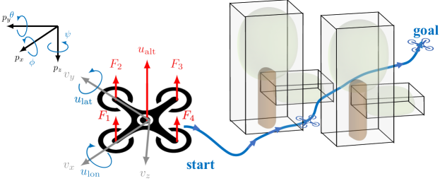
Figure 4: Illustration of the quadcopter state, forces, and moments described in the earth ($p_{x}$, $p_{y}$, $p_{z}$, $\theta$, $\varphi$, $\phi$) and body frame. The considered inputs are the lateral and longitudinal moments are provided by the four rotors resulting in the forces $F_{i}$.

A linearized model, as presented in ⁴⁰ based on a nonlinear dynamic model is used, c.f. Appendix A. The states of the quadcopter are roll and pitch angles $(\phi,\theta)$, roll and pitch rates $(w_{x},w_{y})$, 3D position $(p_{x},p_{y},p_{z})$, and 3D velocities $(v_{x},v_{y},v_{z})$. The linearized model has three inputs: $u_{\text{lon}}=\theta_{c}$, $u_{\text{lat}}=\phi_{c}$ and $u_{\text{alt}}=T_{c}$. The input and states are constrained to:

$$\left[\begin{smallmatrix}-1.5\,\text{m/s}\\ -\pi/4\,\text{rad}\\ -\pi/4\,\text{rad}\end{smallmatrix}\right]\leq\left[\begin{smallmatrix}v_{x},\,v_{y},\,v_{z}\\ \phi,\,\theta,\\ \phi_{c},\,\theta_{c}\end{smallmatrix}\right]\leq\left[\begin{smallmatrix}1.5\,\text{m/s}\\ \pi/4\,\text{rad}\\ \pi/4\,\text{rad}\end{smallmatrix}\right].$$ (20)

The model is discretized with a sampling time of $T_{p}=0.5s$ for the planning problem and $T_{t}=0.05s$, i.e. $M=10$, for the cyclic horizon MPC controller (5). YALMIP ⁴¹ is used to implement and formulate the planning and control problems, exploiting Gurobi ⁴² for the solution of the optimization problems. The required sets are calculated via the MPT toolbox ⁴³.

Figure 5 shows simulations for the case that only a single low layer control mode is used.

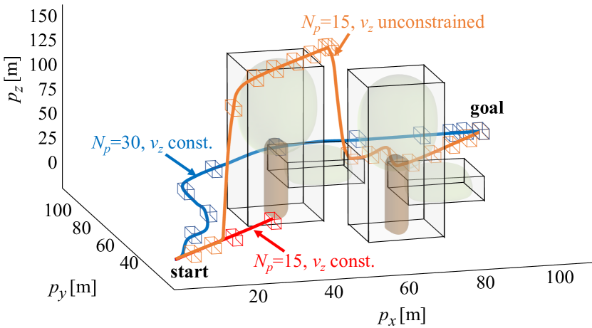
Figure 5: Disturbance free closed-loop simulation results for a single MPC controller mode.

As can be seen, for a small planning horizon of $N_{p}=15$ no path around the obstacle can be found. Only an increase of the planning horizon to $N_{p}=30$, or the removal of the vertical velocity constraint on $v_{z}$ allows the controlled vehicle to reach the goal. Note that in all cases no collisions occur. The (maximum) computation times to solve the planning problem are $\text{T}_{\text{com}}=$ 0.4 s for $N=15$, and $\text{T}_{\text{com}}=$ 60 s for $N=30$, which is well above the desired re-planning time of 0.5 s..

Figure 6 shows simulation results using two operation modes for the low-layer MPC controller. They correspond to a fast operation mode, given by $-1.5\,\text{m/s}\,\leq(v_{x},\,v_{y})\leq 1.5\,\text{m/s}$ and a slow operation mode given by $-1.0\,\text{m/s}\,\leq(v_{x},\,v_{y})\leq 1.0\,\text{m/s}$. The fast operation mode corresponds to a large uncertainty set, while slow operation mode leads to a smaller uncertainty bound $\mathbb{W}_{2}$ and thus smaller sets $\mathbb{E}_{2}$ and $\mathbb{Z}_{2}$.

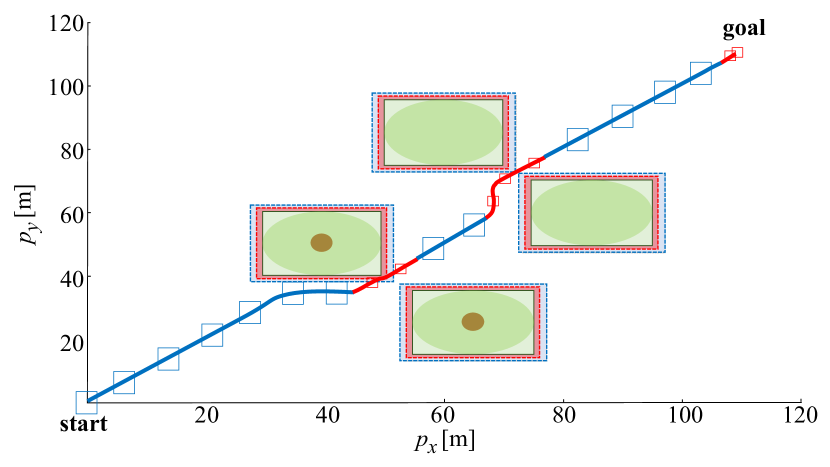
((a)) 3D and top down view.

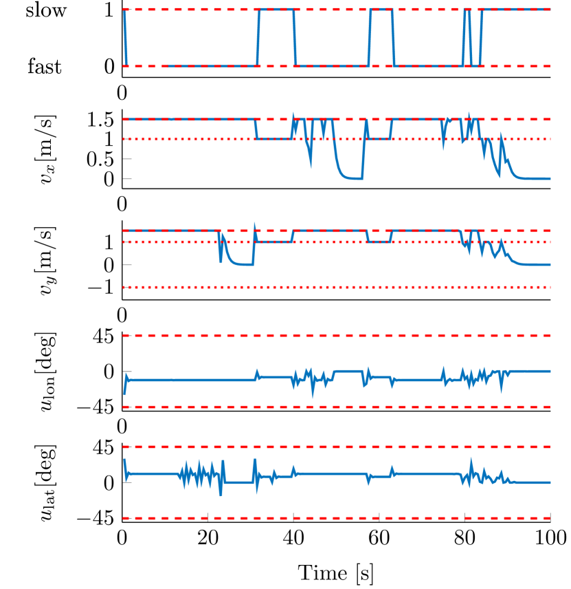
((b)) Selected operation mode, input, and speed profile

Figure 6: (a): Using two operating modes allows the quadcopter to reach the goal on a direct way. (b): The reference planner switches between the two operation modes, resulting in different velocity constraints and uncertainty bounds.

Figure 7 shows simulation results for large wind disturbances, which are not considered in the controller explicitly. As can be seen, the hierarchical control strategy is able to achieve the goal, while avoiding the obstacles and satisfying the input constraints.

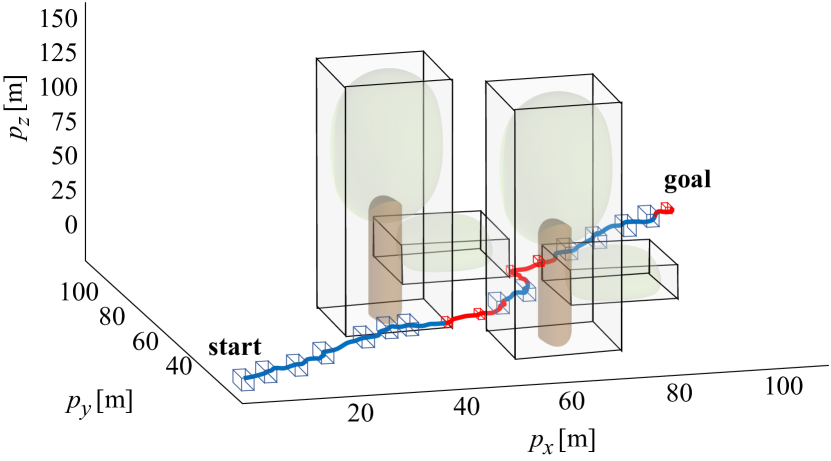
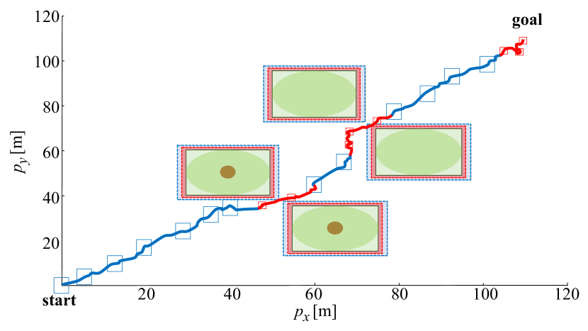
((a)) 3D and top down view.

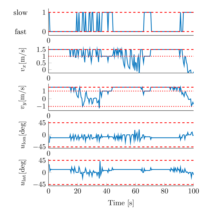
((b)) Selected operation mode, input, and speed profile

Figure 7: (a): Strong wind disturbance case: the reference planner allows to reach the goal and avoid obstacles despite strong wind disturbance. (b): The reference planner switches between the two operation modes, resulting in different velocity constraints and uncertainty bounds.

Summarizing, introducing additional control modes allows avoiding conservative behavior while satisfying constraints and being computationally feasible.

5 Conclusions and outlook

We propose a tightly integrated hierarchical predictive control and planning approach. Both planner and controller repeatedly solve moving horizon optimal control problems. The upper- and lower-layers exploit different “contracts” (guaranteed uncertainty bounds), i.e., the planner can choose other low-layer controller regions/modes instead of using a fixed safety corridor to capture the controller capabilities. For example, the planner can choose slow-speed movement with high precision or a fast speed with large uncertainty bounds.

The planning reference is determined by solving a moving horizon optimization problem considering a simplified model. It exploits constraints tightening, which represents the lower-layer tracking capabilities in the form of the precision contracts. The resulting planning algorithm can be reformulated as a MILP, allowing for efficient and reliable solutions. The low-layer tube-based MPC controller utilizes a cyclic horizon and results in a convex optimization problem. It guarantees constraint satisfaction and the desired tracking accuracy for the different modes. Moreover, it operates at a faster time scale. We derived conditions that ensure compatibility between the planning and control layers to guarantee recursive feasibility and ensure the satisfaction of constraints and obstacle avoidance.

Simulation results demonstrated the efficiency and applicability of the proposed hierarchical strategy. First, the contract option provides significant advantages, e.g.,  it leads to a less conservative solution. Moreover, the hierarchical decomposition of the challenging vehicle control/planning problem leads to a decrease in the computational cost. It allows the implementation of robust control on-board while providing guarantees.

Possible extension are the consideration of ellipsoidal tube MPC methods ^{39, 44}. In this case, the lower controller online sends the tube parameterization to the upper layer. Therefore, the planner can predict a possible uncertainty evaluation over the planning horizon.

We also aim to experimentally evaluate the approach, implementing the upper-layer planner and the lower-layer MPC controller on computationally limited systems.

Appendix A Quadcopter model

The quadcopter states and inputs are represented in two different coordinate systems, e.g., earth and body fixed frame, see Fig. 4. The resulting nonlinear dynamics are given by ⁴⁰:

$$\begin{bmatrix}m_{t}\mathbf{I}_{3\times 3}&{0}\\ {0}&\mathbf{I}\end{bmatrix}\begin{bmatrix}\dot{{V}}\\ {W}\end{bmatrix}+\begin{bmatrix}{W}\times m_{t}{V}\\ {W}\times\mathbf{I}{W}\end{bmatrix}=\begin{bmatrix}{F}\\ {T}\end{bmatrix},$$ (21)

where $m_{t}$ and ${I}$ are the mass and inertia matrix, ${V}$ and ${W}$ are the linear and angular velocities expressed in the body-fixed frame. ${F}$ and ${T}$ are the applied forces and moments. The model is linearized assuming decoupling of the translational and the attitude dynamics ⁴⁰, leading to

$$\dot{x}_{\text{3D}} =A_{\text{3D}}x_{\text{3D}}+B_{\text{3D}}u_{\text{3D}},$$ (22a)

$$y_{\text{3D}} =C_{\text{3D}}x_{\text{3D}}+D_{\text{3D}}u_{\text{3D}},$$ (22b)

with: $x_{\text{3D}}=[x^{\top}_{\text{lon}}\,x^{\top}_{\text{lat}}\,x^{\top}_{\text{alt}}]^{\top},\quad u_{\text{3D}}=[u^{\top}_{\text{lon}}\,u^{\top}_{\text{lat}}\,u^{\top}_{\text{alt}}]^{\top},$ $A_{\text{3D}}=\left[\begin{smallmatrix}A_{\text{lon}}&0&0\\ 0&A_{\text{lat}}&0\\ 0&0&A_{\text{alt}}\end{smallmatrix}\right],$ $B_{\text{3D}}=\left[\begin{smallmatrix}B_{\text{lon}}&0&0\\ 0&B_{\text{lat}}&0\\ 0&0&B_{\text{alt}}\end{smallmatrix}\right].$ The corresponding longitudinal, lateral and vertical sub-dynamics are given by:

$$\dot{x}_{\text{lon}} =A_{\text{lon}}x_{\text{lon}}+B_{\text{lon}}u_{\text{lon}},$$ (23a)

$$\dot{x}_{\text{lat}} =A_{\text{lat}}x_{\text{lat}}+B_{\text{lat}}u_{\text{lat}},$$ (23b)

$$\dot{x}_{\text{alt}} =A_{\text{alt}}x_{\text{alt}}+B_{\text{alt}}u_{\text{alt}},$$ (23c)

with the matrices $A_{\text{lon}}=\left[\begin{smallmatrix}0&1&0&0\\ 0&-\lambda_{x}&-g&0\\ 0&0&0&1\\ 0&0&-a_{w_{x},\theta}&-a_{w_{x},w_{x}}\end{smallmatrix}\right],$ $B_{\text{lon}}=\left[\begin{smallmatrix}0\\ 0\\ 0\\ b_{x}\end{smallmatrix}\right],$ where longitudinal state is $x_{\text{lon}}=[p_{x}\,v_{x}\,\theta\,w_{x}]^{\top}$, with the input $u_{\text{lon}}=\theta_{c}$. The lateral state is $x_{\text{lat}}=[p_{y}\,v_{y}\,\phi\,w_{y}]^{\top}$, with the input $u_{\text{lat}}=\phi_{c}$ and the matrices $A_{\text{lat}}=\left[\begin{smallmatrix}0&1&0&0\\ 0&-\lambda_{y}&g&0\\ 0&0&0&1\\ 0&0&-a_{w_{y},\phi}&-a_{w_{y},w_{y}}\end{smallmatrix}\right],$ $B_{\text{lat}}=\left[\begin{smallmatrix}0\\ 0\\ 0\\ b_{y}\end{smallmatrix}\right].$ Finally, the matrices for vertical (altitude) dynamics are given by $A_{\text{alt}}=\left[\begin{smallmatrix}0&1\\ 0&-\lambda_{z}\end{smallmatrix}\right],$ $B_{\text{alt}}=\left[\begin{smallmatrix}0\\ b_{z}\end{smallmatrix}\right],$with the vertical state $x_{\text{alt}}=[p_{z}\,v_{z}]^{\top}$, and the input is $u_{\text{alt}}=T_{c}$. The overall UAV states are the roll and pitch angles $(\phi,\theta)$, roll and pitch rates $(w_{x},w_{y})$, the positions $(p_{x},p_{y},p_{z})$, and the velocities $(v_{x},v_{y},v_{z})$. The parameters $\lambda_{x},\lambda_{y},\lambda_{z},a_{w_{x},\theta},a_{w_{x},w_{x}},a_{w_{y},\phi},a_{w_{y},w_{y}},b_{x},b_{y},b_{z}$ can be found in ⁴⁰.

References

- 1 Paden B, Čáp M, Yong SZ, Yershov D, Frazzoli E. A survey of motion planning and control techniques for self-driving urban vehicles. IEEE Transactions on intelligent vehicles 2016; 1(1): 33–55.
- 2 Schwarting W, Alonso-Mora J, Rus D. Planning and decision-making for autonomous vehicles. Annual Review of Control, Robotics, and Autonomous Systems 2018; 1: 187–210.
- 3 Dadkhah N, Mettler B. Survey of motion planning literature in the presence of uncertainty: Considerations for UAV guidance. Journal of Intelligent & Robotic Systems 2012; 65(1-4): 233–246.
- 4 Kingston Z, Moll M, Kavraki LE. Sampling-based methods for motion planning with constraints. Annual review of control, robotics, and autonomous systems 2018; 1: 159–185.
- 5 Ibrahim M. Real-Time Moving Horizon Planning and Control of Aerial Systems under Uncertainties. Phd thesis. Otto von Guericke University, Institute for Automation Engineering; 2020.
- 6 Rosolia U, Singletary A, Ames AD. Unified multi-rate control: from low level actuation to high level planning. arXiv preprint arXiv:2012.06558 2020.
- 7 Pant YV, Yin H, Arcak M, Seshia SA. Co-design of control and planning for multi-rotor UAVs with signal temporal logic specifications. In: Proc. American Control Conference. IEEE. ; 2021: 4209–4216.
- 8 Broderick JA, Tilbury DM, Atkins EM. Optimal coverage trajectories for a UGV with tradeoffs for energy and time. Autonomous Robots 2014: 257–271.
- 9 Ibrahim M, Matschek J, Morabito B, Findeisen R. Hierarchical model predictive control for autonomous vehicle area coverage. IFAC-PapersOnLine 2019; 52(12): 79–84.
- 10 Yin H, Bujarbaruah M, Arcak M, Packard A. Optimization based planner–tracker design for safety guarantees. In: Proc. American Control Conference. IEEE. ; 2020: 5194–5200.
- 11 Ibrahim M, Matschek J, Morabito B, Findeisen R. Improved area covering in dynamic environments by nonlinear model predictive path following control. IFAC-PapersOnLine 2019; 52(15): 418–423.
- 12 Koeln J, Alleyne A. Two-Level Hierarchical Mission-Based Model Predictive Control. In: American Control Conference. IEEE. ; 2018: 2332-2337.
- 13 Vermillion C, Menezes A, Kolmanovsky I. Stable hierarchical model predictive control using an inner loop reference model and -contractive terminal constraint sets. Automatica 2014; 50(1): 92–99.
- 14 Goerzen C, Kong Z, Mettler B. A survey of motion planning algorithms from the perspective of autonomous UAV guidance. Journal of Intelligent and Robotic Systems 2010; 57(1-4): 65.
- 15 Quan L, Han L, Zhou B, Shen S, Gao F. Survey of UAV motion planning. IET Cyber-systems and Robotics 2020; 2(1): 14–21.
- 16 Mac TT, Copot C, Tran DT, De Keyser R. Heuristic approaches in robot path planning: A survey. Robotics and Autonomous Systems 2016; 86: 13–28.
- 17 Grüne L, Pannek J. Nonlinear model predictive control. Springer . 2017.
- 18 Findeisen R, Allgöwer F. An introduction to nonlinear model predictive control. 21st Benelux Meeting on Systems and Control 2002; 11: 119–141.
- 19 Rawlings JB, Mayne DQ, Diehl M. Model predictive control: theory, computation, and design. 2. Nob Hill Publishing . 2017.
- 20 Chisci L, Rossiter JA, Zappa G. Systems with persistent disturbances: predictive control with restricted constraints. Automatica 2001; 37(7): 1019–1028.
- 21 Mayne DQ, Seron MM, Raković S. Robust model predictive control of constrained linear systems with bounded disturbances. Automatica 2005; 41(2): 219–224.
- 22 Kögel M, Findeisen R. Stability of NMPC with cyclic horizons. IFAC Proceedings Volumes 2013; 46(23): 809–814.
- 23 Ibrahim M, Kögel M, Kallies C, Findeisen R. Contract-based hierarchical model predictive control and planning for autonomous vehicle. IFAC-PapersOnLine 2020; 53(2): 15758–15764.
- 24 Bäthge T, Kögel M, Di Cairano S, Findeisen R. Contract-based Predictive Control for Modularity in Hierarchical Systems. IFAC-PapersOnLine 2018; 51(20): 499–504.
- 25 Lucia S, Kögel M, Findeisen R. Contract-based predictive control of distributed systems with plug and play capabilities. IFAC-PapersOnLine 2015; 48(23): 205–211.
- 26 Blasi S, Kögel M, Findeisen R. Distributed Model Predictive Control Using Cooperative Contract Options. IFAC-PapersOnLine 2018; 51(20): 448–454.
- 27 Ogata K. Discrete-time control systems. Prentice-Hall . 1995.
- 28 Trodden P, Richards A. Multi-vehicle cooperative search using distributed model predictive control. In: AIAA Guidance, Navigation and Control Conference and Exhibit. AIAA. ; 2008: 7138
- 29 Ibrahim M, Kallies C, Findeisen R. Learning-Supported Approximated Optimal Control for Autonomous Vehicles in the Presence of State Dependent Uncertainties. In: Proc. European Control Conf. IEEE. ; 2020: 338-343.
- 30 Pinto SC, Afonso RJ. Risk Constrained Navigation Using MILP-MPC Formulation. IFAC-PapersOnLine 2017; 50(1): 3586–3591.
- 31 Richards A, How JP. Robust variable horizon model predictive control for vehicle maneuvering. International Journal of Robust and Nonlinear Control: IFAC-Affiliated Journal 2006; 16(7): 333–351.
- 32 Kerrigan EC. Robust constraint satisfaction: Invariant sets and predictive control. Phd thesis. University of Cambridge, Cambridge, UK; 2001.
- 33 Wang Y, Boyd S. Fast model predictive control using online optimization. IEEE Transactions on Control Systems Technology 2009; 18(2): 267–278.
- 34 Zometa P, Kögel M, Findeisen R. AO-MPC: A free code generation tool for embedded real-time linear model predictive control. In: IEEE. ; 2013: 5320–5325.
- 35 Kögel M, Findeisen R. Robust MPC with reduced conservatism by blending multiples tubes. In: Proc. American Control Conference. IEEE. ; 2020.
- 36 Raković SV, Kouvaritakis B, Cannon M, Panos C, Findeisen R. Fully parameterized tube MPC. IFAC Proceedings Volumes 2011; 44(1): 197–202.
- 37 Raković SV. Invention of prediction structures and categorization of robust MPC syntheses. In: IFAC Conf. Nonlinear Model Predictive Control. IFAC. ; 2012: 245–273.
- 38 Kögel M, Findeisen R. Discrete-time robust model predictive control for continuous-time nonlinear systems. In: Proc. American Control Conf. IEEE. ; 2015: 924–930.
- 39 Villanueva ME, Li JC, Feng X, Chachuat B, Houska B. Computing ellipsoidal robust forward invariant tubes for nonlinear MPC. IFAC-PapersOnLine 2017; 50(1): 7175–7180.
- 40 Alexis K, Papachristos C, Siegwart R, Tzes A. Robust model predictive flight control of unmanned rotorcrafts. J. of Intelligent & Robotic Systems 2016; 81(3-4): 443–469.
- 41 Löfberg J. YALMIP: A toolbox for modeling and optimization in MATLAB. In: Proc. IEEE Int. Symp. on Comp. Aided Cont. Syst. Design. IEEE. ; 2004: 284–289.
- 42 Gurobi Optimization, LLC . Gurobi Optimizer Reference Manual. https://www.gurobi.com; 2022.
- 43 Kvasnica M, Grieder P, Baotić M. Multi-Parametric Toolbox (MPT).; 2004.
- 44 Hu H, Feng X, Quirynen R, Villanueva ME, Houska B. Real-time tube MPC applied to a 10-state quadrotor model. In: Proc. American Control Conf. IEEE. ; 2018: 3135–3140.