Determining the seismic age of the young open cluster $\alpha$ Per using $\delta$ Scuti stars

Abstract

In this work we aim at constraining the age of the young open cluster Melotte 20, known as $\alpha$ Per, using seismic indices. The method consists of the following steps: 1) Extract the frequency content of a sample of stars in the field of an open cluster. 2) Search for possible regularities in the frequency spectra of $\delta$ Sct stars candidates, using different techniques, such as the Fourier transform, the autocorrelation function, the histogram of frequency differences and the échelle diagram. 3) Constrain the age of the selected stars by both the physical parameters and seismic indices by comparing them with a grid of asteroseismic models representative of $\delta$ Sct stars. 4) Find possible common ages between these stars to determine the age of the cluster. We performed the pulsation analysis with MultiModes, a rapid, accurate and powerful open-source code, which is presented in this paper. The result is that the age of $\alpha$ Per could be between 96 and 100 Myr. This is an improvement over different techniques in the past. We therefore show that space astroseismology is capable of taking important steps in the dating of young open clusters.

1 Introduction

Open clusters are laboratories of stellar and galactic astrophysics. Having at our disposal a group of tens of stars of similar chemistry and ages, within a narrow field of observation, allows us to better constrain models with which we can compare our observations. We can better characterize the stars in this way, thereby determining their evolutionary stages and, by extension, the origin and evolution of the galaxy to which they belong.

There are many sources that can contribute to ambiguity when determining the age of a cluster by isochrone fitting on the Hertzsprung-Russell (HR) diagram: uncertain distance modulus, cluster membership, binarity of individual stars, reddening and extinction, metallicity, different treatments of the physics of the models used to derive the theoretical isochrones, and the uncertainties from isochrone fitting methods. Ambiguity is even greater in young clusters, with a sparse population of stars leaving the main sequence (turn off). The tip of the red giant branch is used to date globular clusters but cannot be used in young open clusters.

Pulsating stars can allow a better characterization of the cluster, because some of their seismic indices are directly related to internal characteristics of the stars that we want to date. Some types of classical pulsating stars, such as $\delta$ Sct stars, have a rich and varied frequency spectra. They correspond to A and F stars of intermediate mass, very common in the main sequence (MS) for young open clusters. Space missions such as CoRoT (Baglin et al., 2006), Kepler (Koch et al., 2010) and TESS (Ricker et al., 2014) have lowered the detection threshold for their signals. Being grouped around the MS, it is not easy to estimate the age by isochrone fitting. In addition, it has been very difficult, until recently, to find regularities in the frequency spectra of these stars, as in the case of solar-type. There are studies showing that it is possible to find regularities in the frequency pattern of $\delta$ Sct stars, even out of the asymptotic regime (see for example, García Hernández et al., 2009; Paparó et al., 2016; Barceló Forteza et al., 2017; Bedding et al., 2020, and references therein). This is the named large separation, like for solar-type stars, but in the low-order regime (from n=2 to n=8, Suárez et al., 2014). It is defined as the frequency difference between modes of the same degree and consecutive orders:

$$\Delta\nu_{\mathrm{low}}=\nu_{n,\ell}-\nu_{n,\ell-1}$$ (1)

We used here the subscript $low$ to differentiate it from that of the asymptotic regime. However, as for solar-type stars, this $\Delta\nu_{\mathrm{low}}$ is also related to the stellar mean density (Suárez et al., 2014; García Hernández et al., 2015, 2017).

Other seismic indices are the rotational splittings of modes of the same order and degree, related to the angular rotation, and the frequency at maximum power, used in solar-type stars, directly related to the effective temperature, that has also been found in $\delta$ Sct stars (Barceló Forteza et al., 2018, 2020; Bowman & Kurtz, 2018; Hasanzadeh et al., 2021, BF2018, BF2020, BK2018 and H2021 from now on).

Here we use the asteroseismic indices to study the age of the open cluster Melotte 20 (also known as $\alpha$ Per). The structure of the paper is as follows: in Sec. 2 we provide the main characteristics of the cluster and former estimates of its age. In section Sec. 3 we describe the sample of stars used in this research. In Sec. 4 we introduce the code MultiModes, a new tool for the analysis of pulsating stars. In order to show its reliability, we have compared it to one of the most reliable and most used in the field, SigSpec (Reegen, 2007). We explain the details of the code in this section, and also the comparative results obtained between them, using synthetic and real light curves, in terms of accuracy and computing time. In this section we also present the list of $\delta$ Sct stars candidates identified in our sample with the frequency analysis. In Sec. 5 we show how, in four of them, it has been possible to measure the low-order large separation. The angular rotation and the frequency at maximum power of two of these stars have been measured. In Sec. 6 we explain the details of the grid of pulsation models calculated with mesa (Paxton, 2019) and filou (Suárez & Goupil, 2008), in order to constrain the models that better fit to the seismic observations. In Sec. 7 we compare our asteroseismic age with previous works and discuss the reliability of the proposed method to date open clusters. Finally, in Sec. 8, the main conclusions are exposed.

2 $\boldsymbol{\alpha\ P{er}}$

The open cluster $\alpha$ Per is located in the constellation of Perseus, at a distance of $174.89\pm 0.16$ pc, obtained from Gaia DR2 parallaxes (Gaia Collaboration et al., 2018). In Lodieu et al. (2019) a total of 517 astrometric member candidates had been identified in the tidal radius of $\alpha$ Per, using a kinematic method combined with the statistical treatment of parallaxes and proper motions. Netopil & Paunzen (2013) estimated solar metallicity for all members of the cluster and an extinction along the line of sight of around $A_{V}=0.3$ (Prosser, 1992).

Recent age estimates by isochrone fitting range from 20 to 90 Myr. Makarov (2006) estimates the age in around 52 Myr, fitting isochrones in the $M_{V}$ vs. (B-V) diagram, with Z = 0.02, E(B-V) = 0.055, and overshooting computed from the models by Pietrinferni et al. (2004). According to Silaj & Landstreet (2014), the age of $\alpha$ Per is $60\pm 7$ Myr, determined with isochrones by Girardi et al. (2000), with Z = 0.02, fitted onto an HR diagram, considering that the uncertainties are less ambiguous than using a colour-magnitude diagram. Isochrones are most constrained around the one that passes throw the brightest main sequence star, $\psi$ Per (HD 22192), which lies close to the terminal age main sequence (TAMS). In both works, the estimated age of the cluster relies on the parameters of a single star, with a difference of around 8 Myr in their results. Such an approach must be taken with caution, since errors in the estimate of luminosities and temperatures for stars in different evolutionary stages can be quite large. These errors may come from, e.g. the type of photometry to use, bolometric corrections and the correct modulus distance, or even the lack of corrections for rotation effects (see e.g. Suárez et al., 2002, for more details).

Other works use spectroscopic observations of lithium in low-mass stars to estimate the age of young clusters (see for example Basri & Martín (1999), Stauffer et al. (1999)). The idea is that for stars near the substellar mass limit, the age is very sensitive to the lithium depletion boundary, when they start to burn lithium in their cores. As these stars are fully convective in their range of masses, the abundance of lithium is visible in their atmospheres through the 6708 Å Li I doublet. The problem with this method is that unresolved binaries makes the cluster appear younger, as claimed by Martín et al. (2001). For this reason, they used the faintest members to derive the age of the cluster, for which lithium has not been detected. Another difficulty with this method is its dependency on good models that take into account the characteristics of the stellar atmosphere. In Stauffer et al. (1999) the estimated age with this method is around $90\pm 10Myr$, noticeably older than Makarov and Silaj & Landstreet.

Lodieu et al. assumes an age of 90 Myr to compile the census of stars that are members of the cluster, because it is the most common age in the literature.

3 Our sample

Firstly, we have done a cross match between VizieR Online Data Catalogue Gaia DR1 open cluster members (Gaia Collaboration et al., 2017) and TESS Input Catalogue (TIC) (Stassun et al., 2019), searching possible targets belonging to the same open cluster, from which we could obtain light curves from the TESS mission. We have found a list of 112 stars in the field of $\alpha$ Per, with measured values for parallax, mean G magnitude, E($B-V$) reddening, bolometric corrections estimated by Andrae et al. (2018), and effective temperature. They are all contained in the census prepared by Lodieu et al., obtained from Gaia Collaboration et al. (2018). We have estimated the G magnitude with the equation:

$$M_{G}=G-5\log r+5-A_{G},$$ (2)

where the distance $r$ is taken as the inverse of the Gaia parallax. The extinction $A_{G}$ is calculated from reddening values as in Stassun et al.:

$$A_{G}=2.72\,\mathrm{E}(B-V).$$ (3)

The G magnitude is converted to luminosity using the bolometric correction BC(T_eff) with the equation:

$$-2.5\log L=M\textsubscript{G}+\mathrm{BC}\textsubscript{G}(T\textsubscript{eff})-M_{\mathrm{bol}\odot}$$ (4)

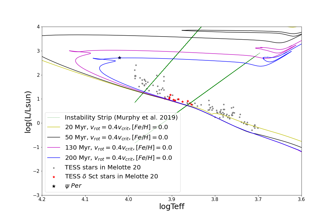
Figure 1 depicts the HR diagram of our sample, including MIST isochrones (Dotter, 2016; Choi et al., 2016; Paxton et al., 2011; Paxton et al., 2013, 2015), with solar metallicity and different ages. They all have been computed from the pre-main sequence phase (PMS) to the end of hydrogen burning. In rotating models, solid-body rotation with $\Omega/\Omega_{crit}=0.4$ is initialized at zero age mean sequence (ZAMS). Rotation makes the star hotter or cooler depending on the efficiency of rotational mixing in the envelope. If rotational mixing introduces a sufficient amount of helium into the envelope, increasing the mean molecular weight, the star becomes more compact and hotter. On the contrary, if rotational mixing is not efficient, the centrifugal effect dominates, making the star cooler and more extended. The ages of the isochrones are taken to cover the wide range of values found in the literature (see previous section). We can see that all the calculated isochrones between 20 and 200 Mrs mostly overlap in the MS zone. We also have located the position of $\psi$ Per on the HR diagram, which is compatible with an age of 200 Myr, quite far from the age estimated by Silaj & Landstreet.

This is where asteroseismology plays an important role, since it provides independent seismic indices that provide an accurate determination of global stellar parameters, including the age of the star.

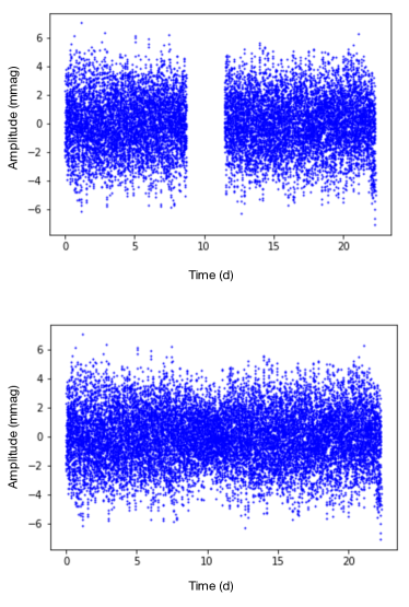
We analyzed a set of 32 stars using data from sector 18 of the TESS mission, with approximately 14700 points, a Rayleigh resolution of approximately 0.045 $d^{-1}$ and a cadence of two minutes. We used the Pre-Search Data Conditioned (PDC) light curves, corrected for instrumental effects, that are publicly available through the MAST. These light curves have a 2.5 days gap caused by the satellite downlink, when the spacecraft passed through the shadow of the Earth at the start of orbit 43 (Fig. 2). Pascual-Granado et al. (2018) showed that the analysis of light curves with gaps can produce an undesirable amount of spurious peaks. Following Pascual-Granado et al. (2015) we interpolated our data using the MIARMA code, which uses autoregressive and moving average models. This method is aimed to preserve the original frequency content of the light curve, making the frequency extraction more reliable than leaving the gaps or using other gap-filling methods.

Figure 1: HR for the sample of 112 stars from the field of $\alpha$ Per, taken from TESS Input Catalogue. Isochrones between 20 and 200 Myr with solar metallicity are taken from MIST. (bluehttp://waps.cfa.harvard.edu/MIST/). The borders of the instability strip are also drawn, calculated according to Murphy et al. (2019). The position of $\psi$ Per is also indicated, one of the most luminous stars in the cluster

Figure 2: Top: Light curve of TIC 252851046. Bottom: Interpolated light curve of TIC 25851046 with MIARMA algorithm

4 Frequency analysis

4.1 MultiModes: a new tool for analysis of pulsating stars

Many of the light curves provided by space missions are uniformly sampled, but show some gaps, due to lack of observations, instrumental issues or environmental effects. The Lomb Scargle Periodogram (from now on LS) is very powerful for analyzing non-uniformly sampled time series (Scargle, 1982). For uniform sampling, LS provides the classical periodogram. The algorithm calculates, at each frequency of interest, a time phase shift, and which in turn is used to evaluate the power spectra at that frequency. This time phase shift makes the LS to be independent of shifting all the points by any constant. In this way, the calculation of LS is equivalent to performing a least squares fit of data to a sinusoidal function for each evaluated frequency. So there is a deep connection between the Fourier Transform and least squares analysis in the LS.

Computing LS can be very slow because it requires a number of calculations of the order of $N^{2}$, $N$ being the number of points in the sample. This problem is partially solved by the implementation of the so-called Fast Lomb Scargle Evaluation (Press & Rybicki, 1989), based on extirpolation from unevenly sampled data.

The width of a peak does not depend on the number of sampled points or the signal to noise ratio (SNR), it only depends on the Rayleigh resolution, which is inversely proportional to the total sample size (VanderPlas, 2018). Two peaks within the Rayleigh resolution, in theory, could not be perfectly resolved by the periodogram. Furthermore, the stochastic nature of the series can cause numerous spurious frequencies to emerge, many of them of low amplitude but above the mean noise level. As detailed in Balona (2014), the problem of using the pre-whitening technique lies in the large number of artificial frequencies that are generated with a high SNR. When, at each step, a signal very similar to the one to be extracted is added to the analyzed light curve, if the fit has not enough accuracy, it can generate an interference pattern around the added frequency.

These spurious frequencies can be avoided, to a great extent, by making a simultaneous fit to all the extracted frequencies, through non-linear optimization. We use least squares fit to a multisine function, taking as parameters the frequencies, amplitudes and phases of each of the peaks to be extracted.

The well-known SigSpec algorithm (Reegen, 2007, SS from now on) uses pre-whitening to extract all those frequencies that are above a certain criterion of significance, defined from the False Alarm Probability (FAP) as:

$$\mathrm{sig}=-\log(\mathrm{FAP})$$ (5)

taking into account the dependency of the FAP with the phases.

Widely used in asteroseismology, it is not open source, and no longer updated.

Inspired by the SigSpec methodology, we developed MultiModes (MM from now on), which is a Python routine developed to extract the most significant peaks of a sample of classical pulsating stars. It is available in a public Github repository and it is customizable. This routine has been designed using the Astropy package to calculate the periodograms and the LMFIT package for non-linear optimization of the extracted signals.

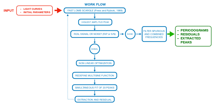
The algorithm (see Fig. 3) fits frequency, amplitude and phase through non-linear optimization, using a multisine function. This function is redefined with the new calculated parameters. It does a simultaneous fit of a number of sinusoidal components (20 are usually enough).

Then they are subtracted from the original signal and the algorithm goes back to the beginning of the loop with the residuals as input, repeating the same process, until the stop criterion is reached. After that, the code can filter suspicious spurious frequencies, those of low amplitude above the Rayleigh resolution, and possible combinations of modes.

4.2 Accuracy test with simulated spectra

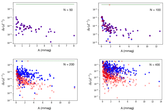
We tested the reliability of MM using synthetic light curves. Following Balona (2014), we constructed artificial light curves with 50, 100, 200 and 400 frequencies, with uniformly distributed values between 0 and 30 d^-1, amplitudes ranging between 0 and 10 mmag, exponentially distributed towards low values, phases uniformly distributed, and adding a Gaussian noise of about 0.5 mmag.

The frequency deviation of MM is similar to that of SS in the curves with 50 and 100 frequencies, around $10^{-4}\ d^{-1}$, when we used an unlimited number of components for the simultaneous fit of the simulated signal (Fig. 4). With a higher number of frequencies, 200 and 400, SS is more accurate than MM by one order of magnitude, because MM used a limited number of components for the simultaneous fit, no more than 50. Still, results with MM have a high enough accuracy for a precise frequency extraction. As the frequency density increases, the problem becomes more unstable since more spurious frequencies appear, with both MM and SS. Therefore, it makes sense to limit the number of components of the simultaneous fit of the light curve when frequency density is very high. In this sense, MM allows us to have greater control over the frequency analysis, by limiting the number of components for the fit, and working with frequency packs.

Figure 3: Workflow of the MultiModes algorithm

Figure 4: Comparative analysis of accuracy between MM and SS, using simulated light curves with different number of frequencies, 50 (upper left panel), 100 (upper right panel), 200 (bottom left panel) and 400 (bottom right panel). Each plot represents the frequency deviation of the extracted peaks with MM (blue filled circles) and SS (red crosses). The dotted green line is the level of the Rayleigh resolution.

4.3 Frequency content of the $\boldsymbol{\delta}$ Scuti sample

From the sample of 32 analysed stars analyzed with MM, we found that 11 of them are $\delta$ Sct stars, or hybrids, a type of pulsating stars with intermediate mass that show low-order acoustic oscillations (p-modes) and also high order gravity modes (g-modes), more typical of $\gamma$ Dor stars (Grigahcène et al., 2010; Uytterhoeven et al., 2011). Except for TIC 252829836 and TIC 347570557, 9 stars in our sample had not been identified as $\delta$ Sct stars so far.

We have analysed the frequency content of these 11 stars using MM and SS, for greater reliability. The frequency comparison assumes that both codes identify the same frequency when their difference is smaller than the Rayleigh resolution. We established the degree or percentage of coincidence based on whether each frequency extracted by MM is among those extracted by SS or not. The degree of coincidence between MM and SS in the values of the extracted frequencies, extracting the most significant frequencies, is above $90\%$ in all the cases (Tab. 1). We have also done a comparative analysis on the computing speed between MM and SS with our sample of 11 $\delta$ Sct stars stars (see Ap. A).

Table 1: Comparative analysis between SS and MM extracted peaks, using ARMA-interpolated light curves with MIARMA code, for the 11 $\delta$ Sct stars sample from $\alpha$ Per. $N$_SSar and $N$_MMar are, respectively, the number of extracted frequencies by SigSpec and MultiModes. SSarMMar is the degree of coincidence between SigSpec and MultiModes

TIC	$N$SSar	$N$MMar	SSarMMar
104319359	249	238	97.9
116011834	233	222	97.7
252829836	82	76	97.4
252851046	213	222	93.7
285935852	45	40	97.5
347570557	189	188	94.7
354638295	97	89	98.9
354792288	55	47	100.0
401079326	39	35	100.0
410732825	69	55	100.0
428320122	71	64	100.0

5 Seismic indices of $\boldsymbol{\delta\ S{cuti}}$ stars

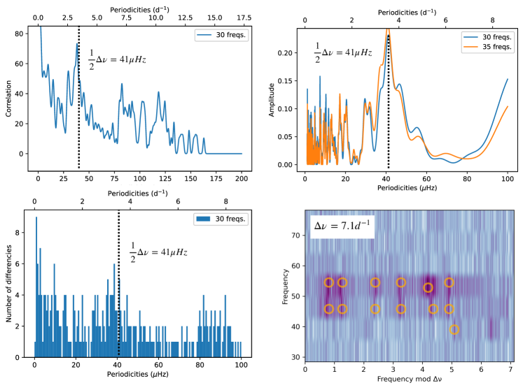
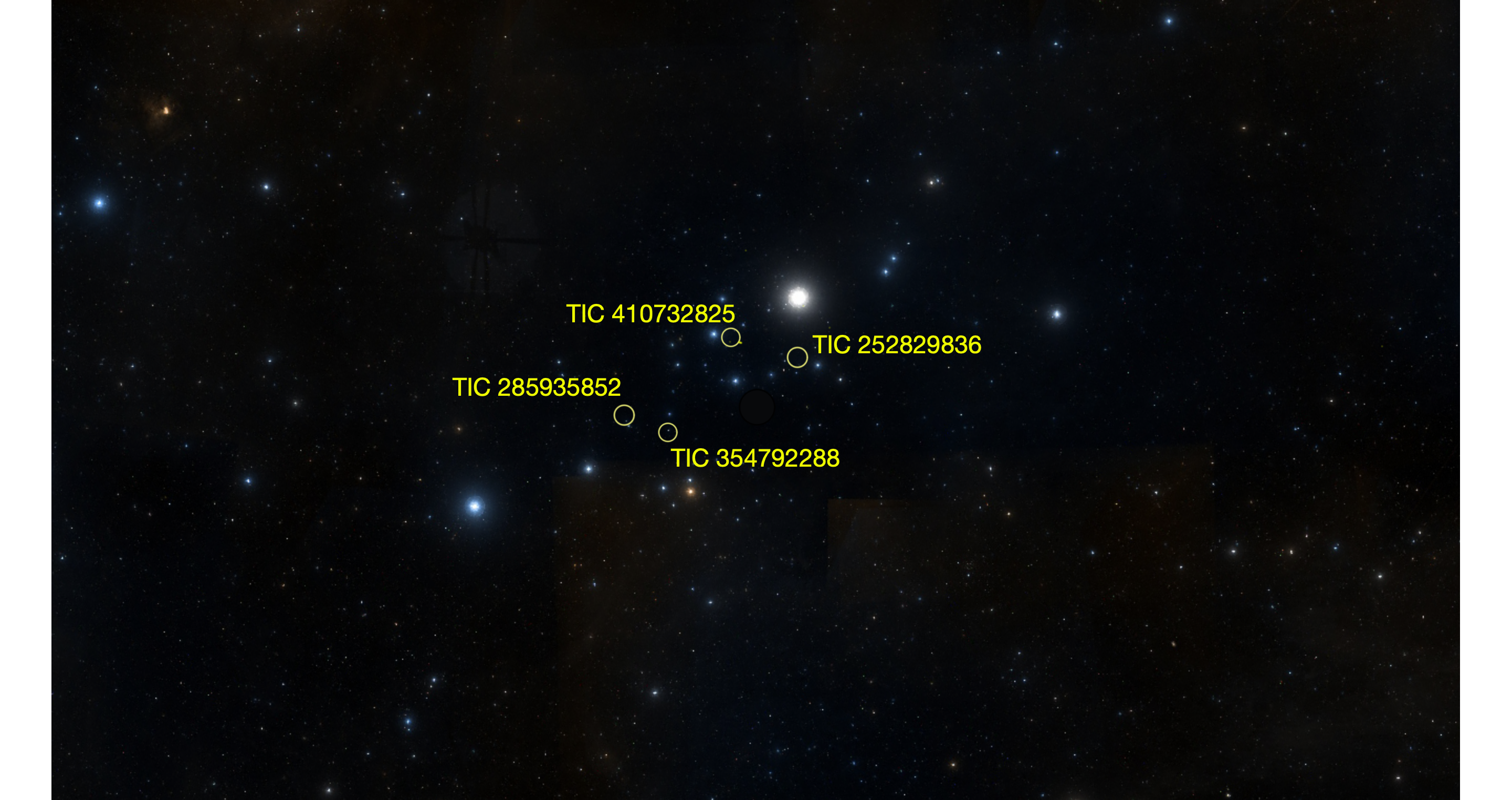
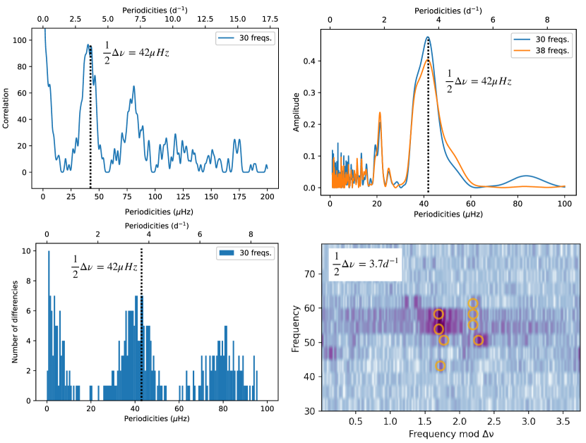
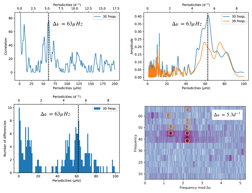
Among our sample of 11 $\delta$ Sct stars, in four of them, TIC 410732825, TIC 354792288, TIC 285935852 and TIC 252829836 (Fig. 5), we found a pattern that we identify as a low-order large separation ($\Delta\nu_{\mathrm{low}}$), following the techniques from García Hernández et al. (2009) and Ramón-Ballesta et al. (2021). The autocorrelation function (AC), the Fourier transform (FT), the histogram of frequency differences (HFD), and the échelle diagram (ED) were applied to the 30 frequencies with highest amplitudes and above 5 $\mbox{d}^{-1}$ to avoid g modes. These frequencies are selected by amplitude but they are given equal amplitudes when computing the transformations.

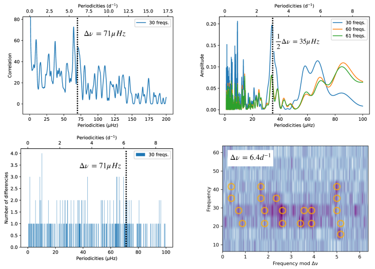
Fig. 3 and Fig. 7 show, respectively, the cases of TIC 354792288 and TIC 410732825 (see the other two stars in Ap. B). For TIC 354792288, the FT, AC and HFD show a peak around $42\ \mu\mathrm{Hz}$. It may be half the value of the low-order large separation. The AC and HFD also show a peak around $84\ \mu\mathrm{Hz}$. The ED shows the alignment of several frequencies when 86 $\mu\mbox{Hz}$ is chosen as the low-order large separation. Thus, we took 84 $\mu\mbox{Hz}$ as $\Delta\nu_{\mathrm{low}}$, being the most common value obtained by the different diagnostic techniques.

We also searched for a pattern connected to the rotational splitting in the p-mode regime. At first order in the perturbative theory, rotation splits the oscillation modes of the same order and spherical degree in the form:

$$\omega_{nlm}=\omega_{nl}+m\Omega(1-C_{L}),$$ (6)

where $\omega$ is the angular frequency, $\Omega$ is the angular rotation frequency and $C_{L}$ is the Ledoux constant, to take into account the effects of the Coriolis force (Aerts et al., 2010). According to Eq. 6, this would allow us to find a pattern corresponding to the rotation frequency in the periodogram, i.e., a regular structure related to $\Omega$. However, this simple distribution of frequencies is only valid for slow rotators. Even at moderate rotations (around 50 $\mathrm{km}~{}\mathrm{s}^{-1}$) the picture changes: rotational splittings are not symmetric anymore and even the m = 0 mode can be displaced (see e.g. Suárez et al., 2006, for more details). These effects may hamper the identification of a rotational splitting.

Nonetheless, some theoretical works computing 2D non-pertubative models and rapid rotation (Reese et al., 2017) combined the AC and the FT (following García Hernández et al., 2009) to search for the patterns of the low-order large frequency separation and the rotational splitting. They pointed out that $\Delta\nu_{\mathrm{low}}$ or its half value comes up usually clearer in the FT, whereas twice the rotational splitting can be better found with AC diagnostic.

From the observational side, Paparó et al. (2016) searched for regularities in the frequency spectra of $\delta$ Sct stars observed by CoRoT using a visual inspection and by means of a semi-automatic algorithm that looks for repeated spacings between frequencies. They claimed that some of these spacings might be not only the large separation but also the rotational splitting or a linear combination of both. The work of Barceló Forteza et al. (2017) used the AC, HFD, ED and DFT of the power spectrum, following the techniques from Régulo & Roca Cortés (2002), to find rotational splittings in a sample of four $\delta$ Sct stars. The main idea was that structural characteristics of the star, such as rotation, alter the power spectra, particularly in the flat plateau, where the density of low amplitude frequencies increases with the rotation rate. Ramón-Ballesta et al. (2021) related regularities found in the frequency spectra of binary $\delta$ Sct stars to their rotational splitting. In their work, they used the FT, the AC and the HFD as in the present research.

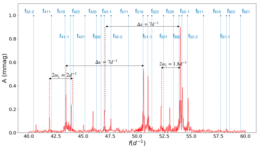
The HFD for two of our stars, TIC 410732825 (Fig. 7) and TIC 285935852 (Fig. A.2) shows a prominent peak around 9-11 $\mu\mbox{Hz}$ that could be the identified as the angular rotation. In fact, Fig. 7 also shows significant peaks at both sides of the one identified as $\Delta\nu_{\mathrm{low}}$, implying the presence of spacings corresponding to the large separation plus and minus the rotational splitting.

In the case of TIC 285935852, Fig. 8 displays the periodogram with the most visible modes, between 40 and 60 $\mu Hz$. It is indicated the low-order large separation, with a value of around $\Delta\nu_{\mathrm{low}}=7d^{-1}$. Some other periodicity can also be noticed that might correspond to twice the rotational splitting of around 0.9-1.0 $d^{-1}$, or equivalently, 9-11 $\mu\mbox{Hz}$. This is consistent with the results by Reese et al. (2017). The $m\neq 0$ modes are not symmetric with respect to the $m=0$ mode, that it is displaced but a spacing corresponding to double the rotational splitting still remains. To check this behaviour, the mode distribution is compared to a compatible model and set of pulsation frequencies computed with the mesa and filou codes (see Sec. 6), taking rotation into account up to second order in the pertubative theory for the adiabatic oscillation computation (including near-degeneracy effects and stellar structure deformation). The mode distribution is similar in both the model and the observation although the limitations of our calculations are clear. Some theoretical modes lie close to the observed ones but others do not. There are missing or completely off modes from the model. Fortunately, the spacings remain although our mode identification might mismatch if we use non-rotating models. We emphasise the importance of taking rotation into account when modelling $\delta$ Sct stars, as also pointed out by Murphy et al. (2021), although they used non-rotating models to carry out a mode identification.

Another seismic index, recently discovered for $\delta$ Sct stars, is the frequency at maximum power, related to the effective temperature of the star, as shown in the works of BF2018, BF2020, BK2018 and H2021. There are different ways of defining the frequency at maximum power. BK2018 defines it with the peak of maximum amplitude in the spectrum, $\nu$_max,0. BF2018 and BF2020 do it in two different ways, one of them with $\nu$_max,0 and the other through the mean of the most significant extracted peaks weighted by their amplitudes, $\nu$_max,w. H2021 do it through the maximum of the autocorrelation of the power spectra, $\nu$_max,2D. As is explained in Hasanzadeh et al. (2021), and with more detail in Viani et al. (2019), the AC method is applied on several windows of the SNR periodogram, to obtain the range of frequencies for the modes’ envelope. Then, a Gaussian curve is fitted to the mean collapsed correlation with each window. The peak of this curve is $\nu$_max,2D.

This relation is very dependent on the evolutionary stage of the star through log g, and it is affected by gravity darkening, as a result of the rapid rotation. This quite large dispersion is probably intrinsic to the relationship itself, and also due to observational errors. The relation probably does not have the same origin as for solar-like stars since the excitation mechanism of the modes is very different in these two types of pulsators.

Tab. 2 shows the values of all these seismic indices that will serve to constrain the models to try to date these four stars accurately, and therefore, the cluster. The uncertainty of $\nu$_max,0 is the error of the single frequency extracted with MM. The uncertainty in the location of $\nu$_max,w has been calculated from the standard deviation of the amplitude weighted data. For $\nu$_max,2D, we have taken the standard deviation of the Gaussian fit as its corresponding error.

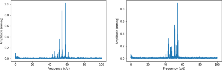
TIC 354792288 and TIC 285935852 show a set of very grouped frequencies between 40 and 60 $\mu\mbox{Hz}$ (Fig. 9), and don’t show significant modes below $5d^{-1}$, which indicates that they can probably be pure $\delta$ Sct stars, as it is defined in Grigahcène et al. (2010); Uytterhoeven et al. (2011). With both stars, we have used $\nu$_max,0 for BF2018’s and BK2018’s relations, $\nu$_max,w for BF2020’s, and $\nu$_max,2D for H2021’s, in order to determine a mean effective temperature, $\widetilde{T}$_eff, (see Tab. 3), considering that the gravity darkening effect due to rotation makes the star hotter on the poles and cooler on the equator. Regarding the uncertainties of the effective temperature, we have calculated them using the error propagation method, from the corresponding errors of $\nu$_max,0, $\nu$_max,w and $\nu$_max,2D and the coefficients of their respective relations.

Figure 5: The four selected targets in the field of $\alpha$ Per  for which we have obtained regularities in the frequency spectra

Figure 6: Measured regularities in the frequency spectra of TIC 354792288. The top left panel represents the autocorrelation diagram (AC) of periodicities calculated with the first 30 frequencies extracted by MM, showing peaks around 42 $\mu$Hz (black dotted line) and 84 $\mu$Hz. Top right, the Fourier transform (FT) for the periodicities of those first 30 frequencies, showing a peak around 42 $\mu$Hz (black dotted line). Bottom left, the histogram of frequency differences (HFD) with the first 30 frequencies, showing peaks around 42 $\mu$Hz (black dotted line) and 84 $\mu$Hz. Bottom right, the echelle diagram (ED) showing two vertical ridges (orange circles) when 1/2$\Delta\nu_{\mathrm{low}}$ is chosen around 3.7 $d^{-1}$, equivalent to 43 $\mu$Hz. ED is done with Python package Echelle 1.5.1, developed by Hey & Ball 2020

Figure 7: Measured regularities in the frequency spectra of TIC 410732825. The autocorrelation diagram (AC) (top left), the Fourier transform (FT) (top right), and the histogram of frequency differences (HFD) (bottom left), calculated with the first 30 frequencies extracted by MM, show a prominent peak around 63 $\mu$Hz (black dotted line). And also, the echelle diagram (ED) (bottom right) show a very clear vertical ridge (orange circles) when $\Delta\nu_{\mathrm{low}}$ is around 5.3 $d^{-1}$, equivalent to 61 $\mu$Hz

Figure 8: Periodogram of TIC 285935852, showing a measured low-order large separation of around $\Delta\nu_{\mathrm{low}}=7d^{-1}$, and a rotational splitting of around red2$\omega_{r}=1.9d^{-1}$. The modes distribution is compared to a suitable model calculated with mesa-filou(see Sec. 6). The blue dotted lines show the positions of some of the theoretical modes, denoted as $f_{nlm}$, where n is the corresponding radial order, l is the spherical degree and m the azimutal order

. Some modes seem to follow the frequency distribution of the model. Others, related to rotation, where the frequency splitting is visible, don’t do it. Even the centroids are displaced from the model

Figure 9: Periodograms for TIC 354792288 and TIC 285935852, showing very grouped frequencies between 40 and 60 $\mu Hz$

Table 2: Seismic indices of the selected targets from $\alpha$ Per to constrain the models, in order to determine its ages

TIC	$\Delta\nu_{\mathrm{low}}(\mu Hz)$	$\omega_{r}(\mu Hz)$	$\nu_{\text{max,0}}(\mu Hz)$	$\nu_{\text{max,w}}(\mu Hz)$	$\nu_{\text{max,2D}}(\mu Hz)$
410732825	$63\pm 1$	$10\pm 1$	-	-	-
354792288	$83\pm 1$	-	$670.587\pm 0.001$	$624\pm 15$	$620\pm 70$
285935852	$82\pm 1$	$10\pm 1$	$625.026\pm 0.001$	$602\pm 40$	$605\pm 70$
252829836	$71\pm 1$	-	-	-	-

Table 3: The different relations between the frequency at maximum power and the mean effective temperature for TIC 354792288 and TIC 285935852. References: ¹Barceló Forteza et al. 2018, ²Bowman & Kurtz 2018, ³Barceló Forteza et al. 2020, ⁴Hasanzadeh et al. 2021

Relation $\nu_{\mathrm{max}}-\widetilde{T}_{\mathrm{eff}}$	$\sigma(\%)$	TIC 354792288 $\widetilde{T}_{\mathrm{eff}}$ (K)	TIC 285935852 $\widetilde{T}_{\mathrm{eff}}$ (K)
${}^{1}(2.39\pm 0.20)\nu_{\mathrm{max,0}}$ ($\mu\mbox{Hz}$) + $(7110\pm 50)$	5.87	[8530:8898]	[8429:8779]
${}^{2}(22.7\pm 4.0)\nu_{\mathrm{max,0}}(d^{-1})$ + $(6819\pm 21)$	-	[7881:8387]	[7808:8282]
${}^{3}(3.5\pm 0.1)\nu_{\mathrm{max,w}}$ ($\mu\mbox{Hz}$) + $(6460\pm 40)$	3.36	[8477:8773]	[8327:8807]
${}^{4}(1.14\pm 0.07)\nu_{\mathrm{max,2D}}+(1.22\pm 0.01)$ (solar units)	-	[8107:8697]	[8076:8662]

6 The grid of models

We have built a grid of 1D stellar models using the code mesa for the evolution, and filou for calculating the oscillation modes, because it takes into account the stellar distortion due to the centrifugal force in the oscillation frequency computation, and rotation up to second order in the perturbation approximation, including near-degeneracy effects. We have taken orders $2\leq n\leq 8$ and degrees $0\leq l\leq 2$, for calculating the low-order large separation of the models (Suárez et al., 2014; Rodríguez-Martín et al., 2020).

Regarding the evolutionary models, we built a grid using the parameters of Tab. 4, delimiting ages between 20 and 200 Myrs. According to Z_base values, we selected the Type2 tables for opacities. For the mixing length parameter we considered $\alpha=2.0$, and a diffusion coefficient for mixing of elements of $D\_mix=1/30$ (Heger et al., 2000). Overshooting was not considered. In total, 24965 models were calculated.

Table 4: Selected values for the parameters of the grid of models built with MESA

Parameter	Range	Step
Age	[20, 200] Myr	1 Myr
M $(M_{\odot})$	[1.6, 2.7]	0.1 $M_{\odot}$
$Z_{0}$	[0.014, 0.020]	0.002
$\Omega/\Omega_{c}$	[0.15, 0.25]	0.05
$\alpha$	2.0	Fixed

7 Seismic determination of the age of $\boldsymbol{\alpha\ P{er}}$

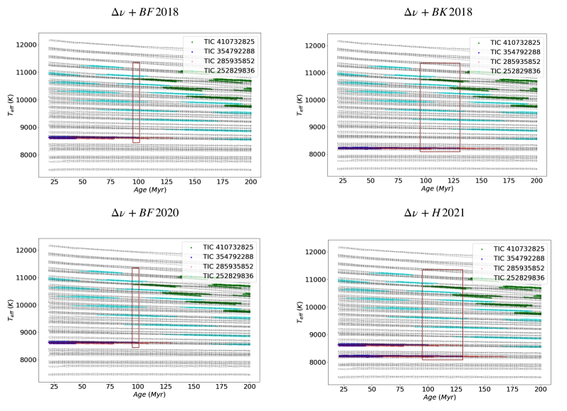
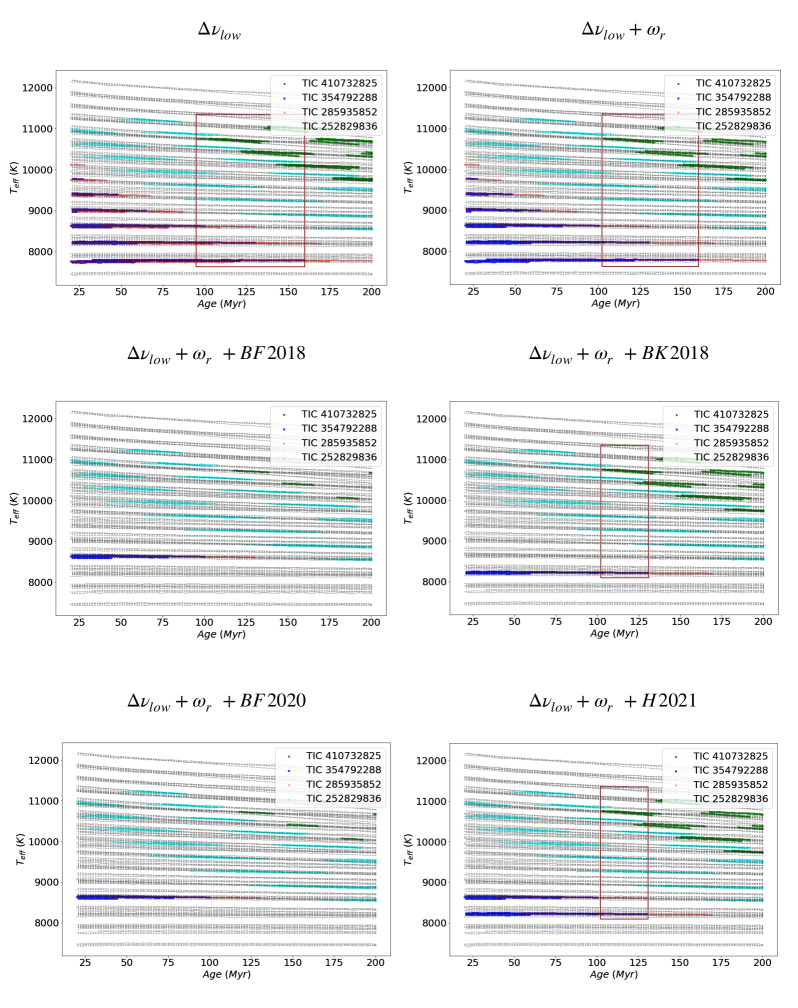
Fig. 10 shows the effective temperature vs age plots for all the calculated models, using the different relations between the frequency at maximum power and the effective temperature presented in Sec. 5. The constrained models for TIC 410732825 are represented in green, for TIC 354792288 in blue, for TIC 285935852 in red and for TIC 252829836 in cyan.

We have compared the observed $\Delta\nu_{\mathrm{low}}$ value with the one calculated directly from the models. If we use the $\nu$_max,0-T_eff relation from BK2018 (top left panel) or $\nu$_max,2D-T_eff from H2021 (bottom left panel), then the constrained models for our four stars show common ages between 96 and 130 Myr. If we use the $\nu$_max,0-T_eff relation from BF2018 (top left panel) or the $\nu$_max,w-T_eff relation from BF2020 (bottom left panel), the result is that the age of the cluster would be between 96 and 100 Myr, not too far from the most common age in the literature, around 90 Myr.

If we add as a constraint the rotation frequency obtained from the splittings in TIC 410732825 and TIC 285935852, then the scenario changes. In Fig. 11 we have plotted effective temperature vs age when using just the low-order large separation (top left panel), when the rotation frequency of both stars are added to constrain the models (top right panel), and also when using the different relations between the frequency at maximum power and the effective temperature (middle and bottom panels). When we have used BK2018 (middle right panel) and H2021 (bottom right panel), two independent works, we obtained the same common ages, between 96 and 130 Myr. However, in the cases of BF2018 and BF2020, the result is that they don’t show common ages.

Tab. 5 shows the observed values of the main parameters of these four stars, and Tab. 6 the values corresponding to the models when using as constraints the low-order large separation and the relation BF2020 (see Fig. 10, bottom left panel). The agreement between the different relationships is greater when we do not constrain the models in rotation. Here we highlight the need to use tighter parameters in models with rotation, such as overshooting or the mixing length parameter, in order to improve the accuracy of the method. We have chosen BF2020 as reference because it was obtained with a quite large sample of pure $\delta$ Sct stars, as can be the case of the two stars with which we have used the relation. BK2018 and H2021 also used hybrid stars, which can impair the accuracy of the method.

Regarding TIC 410732825, the models tell us that it has a larger radius and a lower density than the ones calculated from the observed parameters. The density obtained from the large separation using the García Hernández et al. (2017) relationship seems to corroborate this. The values of the projected rotation of Kounkel et al. (2019) and the seismic rotation are very similar, so the star seems to be equator on. This would explain why the possible values of the observed luminosity are below those of the models. If the observed parameters for TIC 252829836 were correct, then the star would have an age of hundreds of millions of years in order to be compatible with the measured large separation. This solution was therefore discarded, and points toward a wrong estimate of its physical parameters.

Our four stars, which seem to be members of the cluster according to Lodieu et al. (2019), and do not seem to be binary systems, according to Kounkel et al. (2019), point to an age for the cluster of at least 96 Myr.

Table 5: Parameters of the selected targets. References: ¹Stassun et al. 2019, ²Kounkel et al. 2019, ³García Hernández et al. 2017

TIC	$M(M_{\odot})^{1}$	$R(R_{\odot})^{1}$	$\bar{\rho}(\bar{\rho}_{\odot})$	$logg^{1}$	Teff$(K)^{1}$	$log(L/L_{\odot})^{1}$	$vsini(kms^{-1})^{2}$	$\Delta\nu_{\mathrm{low}}(cd^{-1})$	$\bar{\rho}_{\Delta\nu_{\mathrm{low}}}(\bar{\rho}_{\odot})^{3}$
410732825	[1.983:2.651]	[1.592:1.686]	[0.41:0.66]	[4.30:4.45]	[8851:9453]	[1.18:1.28]	[71:107]	[62:64]	[0.31:0.33]
354792288	[1.666:2.370]	[1.518:1.624]	[0.39:0.68]	[4.27:4.44]	[7849:8605]	[0.93:1.08]	[107:119]	[82:84]	[0.54:0.57]
285935852	[1.465:2.063]	[1.545:1.645]	[0.33:0.56]	[4.20:4.36]	[7363:7815]	[0.84:0.92]	[68:73]	[81:83]	[0.53:0.56]
252829836	[1.313:1.863]	[1.617:1.747]	[0.25:0.44]	[4.10:4.27]	[6994:7272]	[0.80:0.84]	[37:39]	[70:72]	[0.39:0.42]

Table 6: Constrained parameters of the models corresponding to our selected targets, using the relation BF2020

TIC	$M(M_{\odot})$	$R(R_{\odot})$	$\bar{\rho}(\bar{\rho}_{\odot})$	log g	Teff(K)	$log(L/L_{\odot})$	$Z_{0}$	$v(kms^{-1})$	$\Delta\nu_{\mathrm{low}}(cd^{-1})$	Age (Myr)
410732825	[2.3:2.6]	[1.94:2.10]	[0.28:0.32]	[4.20:4.24]	[9731:11055]	[1.49:1.75]	[0.016:0.020]	[72:125]	[62:64]	[96:200]
354792288	[1.75:1.85]	[1.51:1.54]	[0.49:0.52]	[4.32:4.34]	[8592:8666]	[1.05:1.06]	[0.016:0.020]	[71:116]	[82:84]	[20:100]
285935852	[1.75:1.85]	[1.51:1.55]	[0.48:0.52]	[4.31:4.33]	[8579:8660]	[1.05:1.07]	[0.016:0.020]	[71:116]	[81:83]	[20:130]
252829836	[1.9:2.6]	[1.68:1.94]	[0.36:0.40]	[4.24:4.30]	[8541:11248]	[1.13:1.71]	[0.016:0.020]	[69:126]	[70:72]	[20:200]

Figure 10: Constrained models for dating ages of the four stars, just using the low regime large separation ($\Delta\nu$), and also adding the different relationships between the frequency at maximum power and the effective temperature: $\Delta\nu+BF2018$, $\Delta\nu+BK2018$, $\Delta\nu+BF2020$ and $\Delta\nu+H2021$

Figure 11: Constrained models for dating ages of the four stars, just using the low regime large separation ($\Delta\nu$), adding the angular rotation for TIC 410732825 and TIC 285935852 ($\Delta\nu+\omega_{r}$) and also adding the different relationships between the frequency at maximum power and the effective temperature: $\Delta\nu+\omega_{r}+BF2018$, $\Delta\nu+\omega_{r}+BK2018$, $\Delta\nu+\omega_{r}+BF2020$ and $\Delta\nu+\omega_{r}+H2021$

8 Conclusions

We have tested an asteroseismic method in order to determine the age of the young open cluster $\alpha$ Per. The technique is based on finding seismic indices, such as the low-order large separation, the frequency at maximum power and the rotation frequency in a sample of 11 $\delta$ Sct stars stars belonging to the field of the cluster. With them we have used the FT, the AC, the HFD and the ED. In four of them, TIC 410732825, TIC 354792288, TIC 285935852 and TIC 252829836 we have measured the low-order regime large separation. With TIC 410732825 and TIC 285935852 we have found evidences of the angular rotation frequency. With the necessary caution, considering that they are near the ZAMS, we have used the relations between the frequency at maximum power and the effective temperature to constrain the age of $\alpha$ Per between 96 and 100 Myr.

The grid we have used can be extended to take into account the variability of parameters such as overshooting, the mixing length parameter or the diffusion of angular momentum.

The estimated age for $\alpha$ Per must be considered with caution until new studies with more $\delta$ Sct stars stars and/or a more detailed modeling allow us to confirm it. In any case, the method based on seismic indices looks like a promising tool for dating young stellar clusters. For the frequency analysis, we have developed a new code, MultiModes, (blueMultiModes), that we present in this paper. The code shows a good reliability after testing it with synthetic light curves, and after being compared with one of the most reliable codes in the field, SigSpec. Moreover, MultiModes is more versatile in terms of frequency analysis control. It has allowed us to find nine previously unknown $\delta$ Sct stars from the original sample of 32 analysed stars.

Data Availability

Tables of the most significant peaks, corresponding to each of the 11 $\delta$ Sct stars of our sample, extracted with MM, are available in blueVizieR DataBase. In them we can find the values of the frequencies, amplitudes, phases, corresponding errors and S/N of the extracted peaks.

List of acronyms

• AC: Autocorrelation Function

• BF2018: Barceló Forteza et al. (2018)

• BF2020: Barceló Forteza et al. (2020)

• BK2018: Bowman & Kurtz (2018)

• DFT: Discrete Fourier Transform

• ED: Èchelle Diagram

• HFD: Histogram of frequency differences

• FT: Fourier Transform

• H2021: Hasanzadeh et al. (2021)

• MM: MultiModes code

• SS: SigSpec code

Appendix A Comparative analysis of efficiency between MM and SS

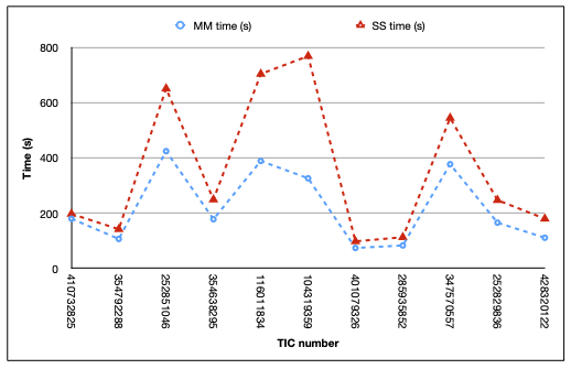
Fig. A.1 represents the executing time of both codes using the light curves of 11 $\delta$ Sct stars stars from our sample. MM is a factor two faster than SS in the cases where the number of extracted peaks is above 200 approximately.

Figure A.1: Comparative analysis of efficiency between MM and SS, in terms of computing time, done with the sample of 11 $\delta$ Sct stars stars

Appendix B Diagrams of regularities of TIC 285935852 and TIC 252829836

We include here the AC, FT, HFD and ED of TIC 285935852 (Fig. A.2) and TIC 252829836 (Fig. A.3), which together with TIC 410732825 (Fig. 7) and TIC 354792288 (Fig. 3), complete the four stars analyzed for which regularities have been found in their corresponding frequency spectra.

Figure A.2: Measured regularities for TIC 285935852

Figure A.3: Measured regularities for TIC 252829836

References

- Aerts et al. (2010) Aerts C., Christensen-Dalsgaard J., Kurtz D. W., 2010, Asteroseismology. Astronomy and Astrophysics Library. ISBN 978-1-4020-5178-4. Springer Science+Business Media B.V., 2010, p.
- Andrae et al. (2018) Andrae R., et al., 2018, A&A, 616, A8
- Baglin et al. (2006) Baglin A., Michel E., Auvergne M., COROT Team 2006, in Proceedings of SOHO 18/GONG 2006/HELAS I, Beyond the spherical Sun. p. 34
- Balona (2014) Balona L. A., 2014, MNRAS, 439, 3453
- Barceló Forteza et al. (2017) Barceló Forteza S., Roca Cortés T., García Hernández A., García R. A., 2017, A&A, 601, A57
- Barceló Forteza et al. (2018) Barceló Forteza S., Roca Cortés T., García R. A., 2018, A&A, 614, A46
- Barceló Forteza et al. (2020) Barceló Forteza S., Moya A., Barrado D., Solano E., Martín-Ruiz S., Suárez J. C., García Hernández A., 2020, A&A, 638, A59
- Basri & Martín (1999) Basri G., Martín E. L., 1999, ApJ, 510, 266
- Bedding et al. (2020) Bedding T. R., et al., 2020, Nature, 581, 147
- Bowman & Kurtz (2018) Bowman D. M., Kurtz D. W., 2018, MNRAS, 476, 3169
- Choi et al. (2016) Choi J., Dotter A., Conroy C., Cantiello M., Paxton B., Johnson B. D., 2016, ApJ, 823, 102
- Dotter (2016) Dotter A., 2016, ApJS, 222, 8
- Gaia Collaboration et al. (2017) Gaia Collaboration et al., 2017, VizieR Online Data Catalog, pp J/A+A/601/A19
- Gaia Collaboration et al. (2018) Gaia Collaboration et al., 2018, A&A, 616, A10
- García Hernández et al. (2009) García Hernández A., et al., 2009, A&A, 506, 79
- García Hernández et al. (2015) García Hernández A., Martín-Ruiz S., Monteiro M. J. P. F. G., Suárez J. C., Reese D. R., Pascual-Granado J., Garrido R., 2015, ApJ, 811, L29
- García Hernández et al. (2017) García Hernández A., et al., 2017, MNRAS, 471, L140
- Girardi et al. (2000) Girardi L., Bressan A., Bertelli G., Chiosi C., 2000, A&AS, 141, 371
- Grigahcène et al. (2010) Grigahcène A., et al., 2010, ApJ, 713, L192
- Hasanzadeh et al. (2021) Hasanzadeh A., Safari H., Ghasemi H., 2021, MNRAS, 505, 1476
- Heger et al. (2000) Heger A., Woosley S. E., Langer N., 2000, New Astron. Rev., 44, 297
- Hey & Ball (2020) Hey D., Ball W., 2020, Echelle: Dynamic echelle diagrams for asteroseismology, doi:10.5281/zenodo.3629933
- Koch et al. (2010) Koch D. G., et al., 2010, ApJ, 713, L79
- Kounkel et al. (2019) Kounkel M., et al., 2019, The Astronomical Journal, 157, 196
- Lodieu et al. (2019) Lodieu N., Pérez-Garrido A., Smart R. L., Silvotti R., 2019, A&A, 628, A66
- Makarov (2006) Makarov V. V., 2006, AJ, 131, 2967
- Martín et al. (2001) Martín E. L., Dahm S., Pavlenko Y., 2001, in von Hippel T., Simpson C., Manset N., eds, Astronomical Society of the Pacific Conference Series Vol. 245, Astrophysical Ages and Times Scales. p. 349
- Murphy et al. (2019) Murphy S. J., Hey D., Van Reeth T., Bedding T. R., 2019, Monthly Notices of the Royal Astronomical Society, 485, 2380
- Murphy et al. (2021) Murphy S. J., Bedding T. R., White T. R., Li Y., Hey D., Reese D., Joyce M., 2021, arXiv e-prints, p. arXiv:2111.04203
- Netopil & Paunzen (2013) Netopil M., Paunzen E., 2013, A&A, 557, A10
- Paparó et al. (2016) Paparó M., Benkő J. M., Hareter M., Guzik J. A., 2016, ApJ, 822, 100
- Pascual-Granado et al. (2015) Pascual-Granado J., Garrido R., Suárez J. C., 2015, A&A, 575, A78
- Pascual-Granado et al. (2018) Pascual-Granado J., Suárez J. C., Garrido R., Moya A., Hernández A. G., Rodón J. R., Lares-Martiz M., 2018, Astronomy and Astrophysics, 614, 1
- Paxton (2019) Paxton B., 2019, Modules for Experiments in Stellar Astrophysics (MESA), doi:10.5281/zenodo.3473377
- Paxton et al. (2011) Paxton B., Bildsten L., Dotter A., Herwig F., Lesaffre P., Timmes F., 2011, ApJS, 192, 3
- Paxton et al. (2013) Paxton B., et al., 2013, ApJS, 208, 4
- Paxton et al. (2015) Paxton B., et al., 2015, ApJS, 220, 15
- Pietrinferni et al. (2004) Pietrinferni A., Cassisi S., Salaris M., Castelli F., 2004, ApJ, 612, 168
- Press & Rybicki (1989) Press W. H., Rybicki G. B., 1989, ApJ, 338, 277
- Prosser (1992) Prosser C. F., 1992, AJ, 103, 488
- Ramón-Ballesta et al. (2021) Ramón-Ballesta A., García Hernández A., Suárez J. C., Rodón J. R., Pascual-Granado J., Garrido R., 2021, MNRAS, 505, 6217
- Reegen (2007) Reegen P., 2007, Astronomy & Astrophysics, 467, 1353
- Reese et al. (2017) Reese D. R., Lignières F., Ballot J., Dupret M.-A., Barban C., van ’t Veer-Menneret C., MacGregor K. B., 2017, Astronomy & Astrophysics, 601, A130
- Régulo & Roca Cortés (2002) Régulo C., Roca Cortés T., 2002, A&A, 396, 745
- Ricker et al. (2014) Ricker G. R., et al., 2014, in Proc. SPIE. p. 914320 (arXiv:1406.0151), doi:10.1117/12.2063489
- Rodríguez-Martín et al. (2020) Rodríguez-Martín J. E., García Hernández A., Suárez J. C., Rodón J. R., 2020, MNRAS, 498, 1700
- Scargle (1982) Scargle J. D., 1982, ApJ, 263, 835
- Silaj & Landstreet (2014) Silaj J., Landstreet J. D., 2014, A&A, 566, A132
- Stassun et al. (2019) Stassun K. G., et al., 2019, The Astronomical Journal, 158, 138
- Stauffer et al. (1999) Stauffer J. R., et al., 1999, ApJ, 527, 219
- Suárez & Goupil (2008) Suárez J. C., Goupil M. J., 2008, Ap&SS, 316, 155
- Suárez et al. (2002) Suárez J. C., Michel E., Pérez Hernández F., Lebreton Y., Li Z. P., Fox Machado L., 2002, A&A, 390, 523
- Suárez et al. (2006) Suárez J. C., Goupil M. J., Morel P., 2006, Astronomy & Astrophysics, 449, 673
- Suárez et al. (2014) Suárez J. C., García Hernández A., Moya A., Rodrigo C., Solano E., Garrido R., Rodón J. R., 2014, A&A, 563, A7
- Uytterhoeven et al. (2011) Uytterhoeven K., et al., 2011, A&A, 534, A125
- VanderPlas (2018) VanderPlas J. T., 2018, ApJS, 236, 16
- Viani et al. (2019) Viani L. S., Basu S., Corsaro E., Ball W. H., Chaplin W. J., 2019, ApJ, 879, 33