Invariance principle and CLT for the spiked eigenvalues of large-dimensional Fisher matrices and applications

Abstract

This paper aims to derive asymptotical distributions of the spiked eigenvalues of the large-dimensional spiked Fisher matrices without Gaussian assumption and the restrictive assumptions on covariance matrices. We first establish invariance principle for the spiked eigenvalues of the Fisher matrix. That is, we show that the limiting distributions of the spiked eigenvalues are invariant over a large class of population distributions satisfying certain conditions. Using the invariance principle, we further established a central limit theorem (CLT) for the spiked eigenvalues. As some interesting applications, we use the CLT to derive the power functions of Roy Maximum root test for linear hypothesis in linear models and the test in signal detection. We conduct some Monte Carlo simulation to compare the proposed test with existing ones.

, , and

t1Corresponding author: Runze Li.

1 Introduction

Motivated by several applications of hypothesis on two-sample covariance matrices and linear hypothesis on regression coefficient matrix in linear models, we consider the following spiked model. Let ${\boldsymbol{\Sigma}}_{1}$ and ${\boldsymbol{\Sigma}}_{2}$ be the covariance matrices from two $p$-dimensional populations, and ${\mathbf{S}}_{1},{\mathbf{S}}_{2}$ be the corresponding sample covariance matrices with sample sizes $n_{1}$ and $n_{2}$. The two-sample spiked model assumes that ${\boldsymbol{\Sigma}}_{2}={\boldsymbol{\Sigma}}_{1}+{\boldsymbol{\Delta}}$, where ${\boldsymbol{\Delta}}$ is a $p\times p$ matrix of finite rank $M$. It is of great interest to study statistical inference on the spikes, including but not limited to, testing the presence of the spikes, testing the number of the spikes, and calculating the power under the alternative hypothesis in two-sample testing problems. Thus, it is critical to establish the asymptotic properties of the spiked eigenvalues of a Fisher matrix ${\mathbf{F}}={\mathbf{S}}_{1}{\mathbf{S}}_{2}^{-1}$. It is of particular interest to derive the asymptotical distribution of $\lambda_{\max}(\mathbf{F})$, the largest eigenvalue of $\mathbf{F}$. In this paper, we first establish an invariance principle for the spiked eigenvalues of the Fisher matrix, and the invariance principle can be used as a universal probability tool to derive the asymptotical distribution of local spectral statistics of $\mathbf{F}$.

The one-sample spiked model ${\boldsymbol{\Sigma}}={\mathbf{I}}_{p}+{\boldsymbol{\Delta}}$ has received a lot of attentions in the literatures, where $\mathbf{I}_{p}$ is the identity matrix, and $\mathbf{\Delta}$ is a low-rank $p\times p$ matrix. Since the seminal work [21], a pioneer work on one-sample spiked model under the setting of the dimension $p$ is of the same order of the sample size $n$, many works have been published and focus on the research of the asymptotic law for the spiked eigenvalues of large-dimensional covariance matrix [6, 2, 7, 26, 11, 24, 25]. Also see [12, 15, 14, 18] for a more general one-sample spiked model. These works establish the limiting distribution for the spiked eigenvalues of the sample covariance matrices under different settings.

Compared with the one-sample spiked model, there are relatively few studies on two-sample spiked model. [35] derived the limiting distribution of the eigenvalues of a Fisher matrix and establish a CLT for a wide class of functionals of all the eigenvalues as a whole. According to [17], the largest eigenvalue of the Fisher matrix follows the Tracy-Widom law under some conditions. Therefore, the results in [35] are not applicable for the local spectral statistics, especially for those made of spiked eigenvalues. For a simplified two-sample spiked models assuming that ${\boldsymbol{\Sigma}}_{1}{\boldsymbol{\Sigma}}_{2}^{-1}$ is a rank $M$ perturbation of identity matrix with diagonal independence and bounded population fourth moment, [33] established CLT for the extreme eigenvalues of large-dimensional spiked Fisher matrices. [23] proposed the rank-one two-sample spiked models that represent the James’ classes in [20], and further derived the asymptotic behavior of the likelihood ratios in large-dimensional setting. The aforementioned works impose some restrictive or unrealistic conditions such as only one threshold, diagonal assumption, rank-one perturbation, etc. The first two conditions (i.e., only one threshold and diagonal assumption) imply that the spiked eigenvalues and non-spiked eigenvalues are generated by independent variables. The assumption of rank-one perturbation means that there is only one spike.

In this paper, we study the asymptotical properties of Fisher matrix of a two-sample spiked model under a new setting, which allows that (a) two populations may have very different covariance matrices, (b) the spiked eigenvalues of the Fisher matrix may be scattered into the spaces of a few bulks, and (c) the largest eigenvalue may tend to infinity. Under this new setting, the fourth moments of population are not required to be bounded. For ease of presentation, we refer to a Fisher matrix with this new setting as a generalized spiked Fisher matrix. Under a general setting, we establish an invariance principle for the generalized spiked Fisher matrix by using a similar but more complicated technique in [18]. With the invariance principle of generalized spiked Fisher matrix, we establish a CLT for the local spiked eigenvalues of a generalized spiked Fisher matrix. As applications, we use the CLT to derive the power functions of Roy maximum root test on linear hypothesis in large-dimensional linear models and the signal detection test.

Compared with existing works on spiked Fisher matrices, this work relaxes the bounded fourth-moment condition on population to a tail probability condition, which is a regular and necessary condition in the weak convergence of the largest eigenvalue. Under the new setting, we establish an invariance principle theorem for the generalized spiked Fisher matrix. With the aid of the invariance principle theorem, we further establish the CLT for the local spiked eigenvalues of large-dimensional generalized spiked Fisher matrices under mild assumptions on the population distribution. As a by-product, our results naturally extend the result of [33] to a general case under which we can successfully remove the diagonal or block-wise diagonal assumption on the matrix ${\boldsymbol{\Sigma}}_{1}{\boldsymbol{\Sigma}}_{2}^{-1}$. Our setting allows that the spiked eigenvalues may be generated from the variables partially dependent on the ones corresponding to the non-spiked eigenvalues. Our setting also allows a few pairs of thresholds for bulks of spiked eigenvalues. In summary, our setting is more realistic than the ones in the existing works.

The rest of this paper is organized as follows. We establish the invariance principle and the CLT of generalized spiked Fisher matrix in Sections 2 and 3, respectively. We use the CLT to derive the local power functions of Roy maximum root test for linear hypothesis in large-dimensional linear models and the test in signal detection in Section 4. We present some numerical study in Section 5. Some technical proofs are given in Section 6. Additional technical proofs are presented in the supplementary material.

2 Invariance principle for spiked generalized Fisher matrix

2.1 Phase transition for the spiked eigenvalues

Suppose that $\check{\mathbf{x}}_{j}$, $j=1,\ldots,n_{1}$ and $\check{\mathbf{y}}_{l}$, $l=1,\ldots,n_{2}$ are random samples from $p$-dimensional populations $\check{\mathbf{x}}$ and $\check{\mathbf{y}}$ with ${\rm E}(\check{\mathbf{x}})={\rm E}(\check{\mathbf{y}})=\mathbf{0}$ and ${\rm Cov}(\check{\mathbf{x}})=\boldsymbol{\Sigma}_{1}$ and ${\rm Cov}(\check{\mathbf{y}})=\boldsymbol{\Sigma}_{2}$, respectively. Define $\mathbf{x}_{j}=\boldsymbol{\Sigma}_{1}^{-1/2}\check{\mathbf{x}}_{j}$ and $\mathbf{y}_{l}=\boldsymbol{\Sigma}_{2}^{-1/2}\check{\mathbf{y}}_{l}$, for $j=1,\cdots,n_{1}$ and $l=1,\cdots,n_{2}$. For ease of presentation, we represent the samples as $\boldsymbol{\Sigma}_{1}^{1/2}\mathbf{X}$ and $\boldsymbol{\Sigma}_{2}^{1/2}\mathbf{Y}$, where $\mathbf{X}=(\mathbf{x}_{1},\cdots,\mathbf{x}_{n_{1}})=(x_{ij})$ and $\mathbf{Y}=(\mathbf{y}_{1},\cdots,\mathbf{y}_{n_{2}})=(y_{il})$ are two independent $p$-dimensional arrays with components having zero mean and identity covariance matrix. To broaden the application of new theory developed in this paper, we allow both $\mathbf{X}$ and $\mathbf{Y}$ to be complex matrix, and denote $\mathbf{A}^{*}$ to be the conjugate transpose of a complex matrix $\mathbf{A}$. Define $\mathbf{T}_{p}=\boldsymbol{\Sigma}_{1}^{1/2}\boldsymbol{\Sigma}_{2}^{-{1/2}}$ and assume that the spectrum of $\mathbf{T}_{p}^{*}\mathbf{T}_{p}$ is formed as

$$\beta_{p,1},\cdots,\beta_{p,j},\cdots,\beta_{p,p}$$ (1)

in descending order. Denote the spikes as $\alpha_{k}:=\beta_{p,j_{k}+1}=\cdots=\beta_{p,j_{k}+m_{k}}$ with $j_{k}$’s being arbitrary ranks in the array (1). All the spikes, $\alpha_{1},\cdots,\alpha_{K}$, with multiplicity $m_{k},k=1,\cdots,K$ are lined arbitrarily in groups among all the eigenvalues, satisfying $m_{1}+\cdots+m_{K}=M$, a fixed integer. Additionally, the spiked eigenvalues are allowed to be extremely larger or smaller than the non-spiked ones, which is useful when considering system fluctuations. Such settings have not been considered in other existing literatures. The corresponding sample covariance matrices of the two observations are

$${\mathbf{S}}_{1}=\frac{1}{n_{1}}\boldsymbol{\Sigma}_{1}^{1\over 2}\mathbf{X}\mathbf{X}^{*}\boldsymbol{\Sigma}_{1}^{1\over 2},\quad{\mathbf{S}}_{2}=\frac{1}{n_{2}}\boldsymbol{\Sigma}_{2}^{1\over 2}\mathbf{Y}\mathbf{Y}^{*}\boldsymbol{\Sigma}_{2}^{1\over 2},$$ (2)

respectively. We will investigate the eigenvalues of the generalized spiked Fisher matrix $\mathbf{F}=\mathbf{S}_{1}\mathbf{S}_{2}^{-1}=\boldsymbol{\Sigma}_{1}^{1/2}\tilde{\mathbf{S}}_{1}\boldsymbol{\Sigma}_{1}^{1/2}\boldsymbol{\Sigma}_{2}^{-{1/2}}\tilde{\mathbf{S}}_{2}^{-1}\boldsymbol{\Sigma}_{2}^{-{1/2}}$, where ${\tilde{\mathbf{S}}}_{1}=(1/n_{1})\mathbf{X}\mathbf{X}^{*}$ and ${\tilde{\mathbf{S}}}_{2}=({1}/{n_{2}})\mathbf{Y}\mathbf{Y}^{*}$ are the standardized sample covariance matrices, respectively. It is well known that the eigenvalues of $\mathbf{F}$ are the same of the matrix with the form (Still use $\mathbf{F}$ for brevity, if no confusion):

$$\mathbf{F}=\mathbf{T}_{p}^{*}{\tilde{\mathbf{S}}}_{1}\mathbf{T}_{p}{\tilde{\mathbf{S}}}_{2}^{-1}.$$ (3)

Define the singular value decomposition of ${\mathbf{T}}_{p}$ as

$$\mathbf{T}_{p}=\mathbf{U}\left(\begin{array}[]{cc}{\mathbf{D}}_{1}^{1\over 2}&{\bf 0}\\ {\bf 0}&{\mathbf{D}}_{2}^{1\over 2}\end{array}\right){\mathbf{V}}^{*},$$ (4)

where $\mathbf{U},\mathbf{V}$ are unitary matrices (orthogonal matrices for real case), ${\mathbf{D}}_{1}$ is a diagonal matrix of the $M$ spiked eigenvalues of the generalized spiked Fisher matrix $\mathbf{F}$, and ${\mathbf{D}}_{2}$ is the diagonal matrix of the non-spiked ones with bounded components.

Let $\mathcal{J}_{k}=\{j_{k}+1,\cdots,j_{k}+m_{k}\}$ be the set of ranks of $\alpha_{k}$ with multiplicity $m_{k}$ among all the eigenvalues of $\mathbf{T}_{p}^{*}\mathbf{T}_{p}$. Set the sample eigenvalues of the generalized spiked Fisher matrix $\mathbf{F}$ in the descending order as $l_{p,1}(\mathbf{F}),\cdots,l_{p,j}(\mathbf{F}),\cdots,l_{p,p}(\mathbf{F})$. To derive the limiting law for the spiked eigenvalues of $\mathbf{F}$, we impose some conditions as follow.

Assumption 1 The two double arrays $\{x_{ij},i,j=1,2,...\}$ and $\{y_{ij},i,j=1,2,...\}$ consist of independent and identically distributed (i.i.d.) random variables with mean 0 and variance 1. Furthermore, ${\rm E}x_{ij}^{2}=0$ and ${\rm E}y_{ij}^{2}=0$ hold for the complex case if the variables and ${\bf T}_{p}$ are complex.

Assumption 2. Assuming that $c_{n_{1}}\!=\!p/n_{1}\in(0,\infty)$, $c_{n_{2}}\!=\!p/n_{2}\in(0,1)$ is considered throughout the paper when $\min(p,n_{1},n_{2})\rightarrow\infty$. The matrix $\mathbf{T}_{p}=\boldsymbol{\Sigma}_{1}^{1/2}\boldsymbol{\Sigma}_{2}^{-{1/2}}$ is non-random and the empirical spectral distribution of $\{\mathbf{T}_{p}^{*}\mathbf{T}_{p}\}$ excluding the spikes, $H_{n}(t)$, tends to proper probability measure $H(t)$ if $\min(p,n_{1},n_{2})\rightarrow\infty$. (Dandan: why $c_{2}$ has to be in (0,1))

Assumption 3. Assume $\lim\limits_{\tau\rightarrow\infty}\tau^{4}{\rm P}\left(|x_{11}|>\tau\right)=0$ and $\lim\limits_{\tau\rightarrow\infty}\tau^{4}{\rm P}\left(|y_{11}|>\tau\right)$ $=0$ for the i.i.d. samples, where both of the fourth-moments are not necessarily required to exist.

Assumption 4 Suppose that

$$\max\limits_{t,s}|u_{ts}|^{2}\big{[}{\rm E}\{|x_{11}|^{4}{\delta}(|x_{11}|<\eta_{n_{1}}\sqrt{n_{1}})\}-{\mu_{1}}\big{]}\rightarrow 0,$$

$$\max\limits_{t,s}|v_{ts}|^{2}\big{[}{\rm E}\{|y_{11}|^{4}\delta(|y_{11}|<\eta_{n_{2}}\sqrt{n_{2}})\}-{\mu_{2}}\big{]}\rightarrow 0,$$

where for some constants $\mu_{1}$ and $\mu_{2}$, $\delta(\cdot)$ is the indicator function and $\mathbf{U}_{1}=(u_{ts})$, $\mathbf{V}_{1}=(v_{ts})$ are the first $M$ columns of matrix $\mathbf{U}$ and $\mathbf{V}$ defined in (4), respectively.

Assumption 5 The spiked eigenvalues of the matrix $\mathbf{F}$, $\alpha_{1},\cdots,\alpha_{K}$, with multiplicities $m_{1},\cdots,$ $m_{K}$ laying outside the support of $H(t)$, satisfy $\psi^{\prime}(\alpha_{k})>0,$ for $1\leq k\leq K$, where

$$\psi_{k}:=\psi(\alpha_{k})=\frac{\alpha_{k}\left\{1-c_{1}\int t/(t-\alpha_{k})\mbox{d}H(t)\right\}}{1+c_{2}\int\alpha_{k}/(t-\alpha_{k})\mbox{d}H(t)}$$ (5)

is the limit of the distant sample spiked eigenvalues of a generalized spiked Fisher matrix.

The limit in (5) is derived by [19] when $x_{ij}$ and $y_{ij}$ have bounded fourth moments, and is detailed in the following proposition.

Proposition 2.1.

For any spiked eigenvalue $\alpha_{k}$ with multiplicity $m_{k},k=1,\cdots,K$ of $\mathbf{F}$ defined in (3), let

$$\rho_{k}=\left\{\begin{array}[]{cl}\psi(\alpha_{k}),&\mbox{ if }\psi^{\prime}(\alpha_{k})>0;\\ \psi(\underline{\alpha}_{k}),&\mbox{ if there exists }\underline{\alpha}_{k}\mbox{ such that }\psi^{\prime}(\underline{\alpha}_{k})=0,\mbox{ and }\psi^{\prime}(t)<0,\mbox{ for all }\alpha_{k}\leq t<\underline{\alpha}_{k};\\ \psi(\overline{\alpha}_{k}),&\mbox{ if there exists }\overline{\alpha}_{k}\mbox{ such that }\psi^{\prime}(\underline{\alpha}_{k})=0,\mbox{ and }\psi^{\prime}(s)<0,\mbox{ for all }\overline{\alpha}_{k}<s\leq\alpha_{k},\end{array}\right.$$

where $\psi(\alpha_{k})$ is defined in (5). Then under the Assumptions 1-2, and the bounded fourth-moment assumption, it holds that for all $j\in\mathcal{J}_{k}$, $\{l_{p,j}\}$ almost surely that $\{l_{p,j}/\rho_{k}-1\}$ converges to 0.

Since the convergence of $c_{n_{1}}\to c_{1}$, $c_{n_{2}}\to c_{2}$ and $H_{n}(t)\to H(t)$ may be very slow, the difference $\sqrt{n}(l_{p,j}-\psi_{k})$ may not have a limiting distribution. Thus, we use

$$\psi_{n,k}:=\psi_{n}(\alpha_{k})=\frac{\alpha_{k}\left\{1-c_{n_{1}}\int t/(t-\alpha_{k})\mbox{d}H_{n}(t)\right\}}{1+c_{n_{2}}\int\alpha_{k}/(t-\alpha_{k})\mbox{d}H_{n}(t)},$$

instead of $\psi_{k}$ in $\rho_{k}$, and $n$ denotes $(n_{1},n_{2})$, especially the case of CLT. Then, we only require $c_{n_{1}}=p/n_{1};c_{n_{2}}=p/n_{2}$, and both the dimensionality $p$ and the sample sizes $n_{1},n_{2}$ grow to infinity simultaneously, but not necessarily in proportion.

Note that the Proposition 2.1 holds under the bounded fourth-moment assumption. To relax the bounded fourth-moment assumption to Assumption 3 on the tail probability, we introduce the following truncation procedures.

Let $\delta(A)$ be the indication of set $A$. Let $\hat{x}_{ij}=x_{ij}\delta(|x_{ij}|<\eta_{n_{1}}\sqrt{n_{1}})$, $\tilde{x}_{ij}=(\hat{x}_{ij}-{\rm E}\hat{x}_{ij})/\sigma_{n_{1}}$ and $\hat{y}_{ij}=y_{ij}\delta(|y_{ij}|<\eta_{n_{2}}\sqrt{n_{2}})$, $\tilde{y}_{ij}=(\hat{y}_{ij}-{\rm E}\hat{y}_{ij})/\sigma_{n_{2}}$, where $\sigma_{n_{1}}^{2}=$ ${\rm E}\left|\hat{x}_{ij}-{\rm E}\hat{x}_{ij}\right|^{2}$ and $\sigma_{n_{2}}^{2}=$ ${\rm E}\left|\hat{y}_{ij}-{\rm E}\hat{y}_{ij}\right|^{2}$. By the related techniques of the proofs in Supplement B of [18], we can show that it is equivalent to replace the entries of $x_{ij},y_{ij}$ with their corresponding truncated and centralized variables by Assumption 3. In addition, the convergence rates of arbitrary moments of $\tilde{x}_{ij}$ and $\tilde{y}_{ij}$ are the same as the ones depicted in Lemma C.1 in [18]. Therefore, it is reasonable to consider the generalized spiked Fisher matrix $\mathbf{F}=\mathbf{S}_{1}\mathbf{S}_{2}^{-1}$, which is generated from the entries truncated at $\eta_{n_{1}}\sqrt{n_{1}}$ for $x_{ij}$ and $\eta_{n_{2}}\sqrt{n_{2}}$ for $y_{ij}$, centralized and renormalized. For simplicity, we assume that $|x_{ij}|<\eta_{n_{1}}\sqrt{n_{1}},|y_{ij}|<\eta_{n_{2}}\sqrt{n_{2}}$, ${\rm E}x_{ij}={\rm E}y_{ij}=0,{\rm E}|x_{ij}|^{2}={\rm E}|y_{ij}|^{2}=1$ for the real case and Assumption 3 is satisfied. But for the complex case, the truncation and renormalization cannot reserve the requirement of ${\rm E}x_{ij}^{2}={\rm E}y_{ij}^{2}=0$. However, one may prove that ${\rm E}x_{ij}^{2}=o(n_{1}^{-1})$ and ${\rm E}y_{ij}^{2}=o(n_{2}^{-1})$. By the truncation procedures, the Proposition 2.1 still holds in probability without the bounded fourth-moment assumption if the Assumption 3 is satisfied.

2.2 Invariance principle theorem

For the generalized spiked Fisher matrix $\mathbf{F}=\mathbf{T}_{p}^{*}{\tilde{\mathbf{S}}}_{1}\mathbf{T}_{p}{\tilde{\mathbf{S}}}_{2}^{-1}$ defined in (3), we consider the arbitrary sample spiked eigenvalue of $\mathbf{F}$, $l_{p,j},j\in\mathcal{J}_{k},k=1,\ldots,K$. By the singular value decomposition of $\mathbf{T}_{p}$ in (4) and the eigen-equation for $\mathbf{F}$, we have

$$0=|l_{p,j}\mathbf{I}-\mathbf{F}|=\left|l_{p,j}\mathbf{I}-\mathbf{V}\left(\begin{array}[]{cc}\mathbf{D}^{1\over 2}_{1}&{\bf 0}\\ {\bf 0}&\mathbf{D}^{1\over 2}_{2}\end{array}\right)\mathbf{U}^{*}{\tilde{\mathbf{S}}}_{1}\mathbf{U}\left(\begin{array}[]{cc}\mathbf{D}^{1\over 2}_{1}&{\bf 0}\\ {\bf 0}&\mathbf{D}^{1\over 2}_{2}\end{array}\right)\mathbf{V}^{*}{\tilde{\mathbf{S}}}^{-1}\right|.$$

It is equivalent to

$$0 = |l_{p,j}{\mathbf{V}}^{*}{\mathbf{V}}-{\rm diag}({\mathbf{D}}_{1}^{1\over 2},{\mathbf{D}}_{2}^{1\over 2}){\mathbf{U}}^{*}{\tilde{\mathbf{S}}}_{1}{\mathbf{U}}{\rm diag}({\mathbf{D}}_{1}^{1\over 2},{\mathbf{D}}_{2}^{1\over 2})|$$

$$= \Bigg{|}\begin{pmatrix}l_{p,j}{\mathbf{V}}_{1}^{*}{\tilde{\mathbf{S}}}_{2}{\mathbf{U}}_{1},&l_{p,j}{\mathbf{V}}_{1}^{*}{\tilde{\mathbf{S}}}_{2}{\mathbf{V}}_{2}\\ l_{p,j}{\bf V}_{2}^{*}{\tilde{\mathbf{S}}}_{2}{\mathbf{V}}_{1},&l_{p,j}{\mathbf{V}}_{2}^{*}{\tilde{\mathbf{S}}}_{2}{\bf V}_{2}\end{pmatrix}-\begin{pmatrix}{\mathbf{D}}_{1}^{1\over 2}{\mathbf{U}}_{1}^{*}{\tilde{\mathbf{S}}}_{1}{\mathbf{U}}_{1}\mathbf{D}_{1}^{1\over 2},&{\mathbf{D}}_{1}^{1\over 2}{\mathbf{U}}_{1}^{*}{\tilde{\mathbf{S}}}_{1}\mathbf{D}_{2}^{1\over 2}\\ \mathbf{D}_{2}^{1\over 2}\mathbf{U}_{2}^{*}{\tilde{\mathbf{S}}}_{1}\mathbf{U}_{1}\mathbf{D}_{1}^{1\over 2},&\mathbf{D}_{2}^{1\over 2}\mathbf{U}_{2}^{*}{\tilde{\mathbf{S}}}_{1}\mathbf{D}_{2}^{1\over 2}\end{pmatrix}\Bigg{|}.$$

If we consider $l_{p,j}$ as an sample spiked eigenvalue of $\mathbf{F}$, but not of $\mathbf{D}_{2}^{1/2}\mathbf{U}_{2}^{*}{\tilde{\mathbf{S}}}_{1}\mathbf{U}_{2}\mathbf{D}_{2}^{1/2}$ $\cdot(\mathbf{V}_{2}^{*}\tilde{{\bf S}_{2}}\mathbf{V}_{2}\!)\!^{-1}$, then the following equation holds for every sample spiked eigenvalue, $l_{p,j},j\in\mathcal{J}_{k},k=1,\cdots,K$

$$0= \Big{|}l_{p,j}\mathbf{V}_{1}^{*}{\tilde{\mathbf{S}}}_{2}\mathbf{V}_{1}-\mathbf{D}_{1}^{1\over 2}\mathbf{U}_{1}^{*}{\tilde{\mathbf{S}}}_{1}\mathbf{U}_{1}\mathbf{D}_{1}^{1\over 2}-(l_{p,j}\mathbf{V}_{1}^{*}{\tilde{\mathbf{S}}}_{2}\mathbf{V}_{2}-\mathbf{D}_{1}^{1\over 2}\mathbf{U}_{1}^{*}{\tilde{\mathbf{S}}}_{1}\mathbf{U}_{2}\mathbf{D}_{2}^{1\over 2})\mathbf{Q}^{-{1\over 2}}$$ (6)

$$\!\cdot\!(l_{p,j}\mathbf{I}\!-\!\mathbf{Q}^{-{1\over 2}}\mathbf{D}_{2}^{1\over 2}\!\mathbf{U}_{2}^{*}{\tilde{\mathbf{S}}}_{1}\mathbf{U}_{2}\mathbf{D}_{2}^{1\over 2}\mathbf{Q}^{-{1\over 2}})^{-1}\mathbf{Q}^{-{1\over 2}}(l_{p,j}\mathbf{V}_{2}^{*}{\tilde{\mathbf{S}}}_{2}\mathbf{V}_{1}\!-\!\mathbf{D}_{2}^{1\over 2}\mathbf{U}_{2}^{*}{\tilde{\mathbf{S}}}_{1}\mathbf{U}_{1}\mathbf{D}_{1}^{1\over 2})\Big{|},$$

$$= \bigg{|}\frac{l_{p,j}}{n_{2}}\mathbf{V}_{1}^{*}\mathbf{Y}\mathbf{Y}^{*}\mathbf{V}_{1}-\frac{l_{p,j}^{2}}{n_{2}^{2}}\mathbf{V}_{1}^{*}\mathbf{Y}\mathbf{Y}^{*}\mathbf{V}_{2}\mathbf{Q}^{-{1\over 2}}(l_{p,j}\mathbf{I}-\tilde{\mathbf{F}}\big{)}^{-1}\mathbf{Q}^{-{1\over 2}}\mathbf{V}_{2}^{*}\mathbf{Y}\mathbf{Y}^{*}\mathbf{V}_{1}$$

$$-\frac{l_{p,j}}{n_{1}}\mathbf{D}_{1}^{1\over 2}\mathbf{U}_{1}^{*}\mathbf{X}\big{(}l_{p,j}\mathbf{I}-\underline{\tilde{\mathbf{F}}}\big{)}^{-1}\mathbf{X}^{*}\mathbf{U}_{1}\mathbf{D}_{1}^{1\over 2}$$

$$+\frac{l_{p,j}}{n_{2}}\mathbf{V}_{1}^{*}\mathbf{Y}\mathbf{Y}^{*}\mathbf{V}_{2}\mathbf{Q}^{-{1\over 2}}\big{(}l_{p,j}\mathbf{I}-\tilde{\mathbf{F}}\big{)}^{-1}\mathbf{Q}^{-{1\over 2}}\frac{1}{n_{1}}\mathbf{D}_{2}^{1\over 2}\mathbf{U}_{2}^{*}\mathbf{X}\mathbf{X}^{*}\mathbf{U}_{1}\mathbf{D}_{1}^{1\over 2}$$

$$+\frac{l_{p,j}}{n_{1}}\mathbf{D}_{1}^{1\over 2}\mathbf{U}_{1}^{*}\mathbf{X}\mathbf{X}^{*}\mathbf{U}_{2}\mathbf{D}_{2}^{1\over 2}\mathbf{Q}^{-{1\over 2}}(l_{p,j}\mathbf{I}-\tilde{\mathbf{F}})^{-1}\mathbf{Q}^{-{1\over 2}}\frac{1}{n_{2}}\mathbf{V}_{2}^{*}\mathbf{Y}\mathbf{Y}^{*}\mathbf{V}_{1}\bigg{|},$$

$$= \bigg{|}\{\psi_{n,k}+c_{2}\psi^{2}_{n,k}m(\psi_{n,k})\}\mathbf{I}_{M}+\psi_{n,k}\underline{m}(\psi_{n,k})\mathbf{D}_{1}+\frac{1}{\sqrt{p}}\gamma_{kj}\psi_{n,k}\mathbf{I}_{M}$$

$$\quad+\mathbf{B}_{1}(l_{p,j})+\mathbf{B}_{2}(l_{p,j})+\frac{\psi_{n,k}}{\sqrt{p}}\boldsymbol{\Omega}_{M}(\psi_{n,k},\mathbf{X},\mathbf{Y})+o(\frac{\psi_{n,k}}{\sqrt{p}})\bigg{|},$$ (7)

where $\mathbf{Q}=\mathbf{V}_{2}^{*}{\tilde{\mathbf{S}}}_{2}\mathbf{V}_{2}$, and $\tilde{\mathbf{F}}$ and $\underline{\tilde{\mathbf{F}}}$ are defined as

$$\tilde{\mathbf{F}}=\displaystyle\frac{1}{n_{1}}\mathbf{Q}^{-{1\over 2}}\mathbf{D}_{2}^{1\over 2}{\bf U}_{2}^{*}\mathbf{X}\mathbf{X}^{*}\mathbf{U}_{2}\mathbf{D}_{2}^{1\over 2}\mathbf{Q}^{-{1\over 2}},\quad\underline{{\tilde{\mathbf{F}}}}=\displaystyle\frac{1}{n_{1}}\mathbf{X}^{*}\mathbf{U}_{2}\mathbf{D}_{2}^{1\over 2}\mathbf{Q}^{-1}\mathbf{D}_{2}^{1\over 2}\mathbf{U}_{2}^{*}\mathbf{X};$$ (8)

$\psi_{n,k}$ is used instead of $\psi_{k}$ to avoid the slow convergence as mentioned in Section 2.1, $\gamma_{kj}=\sqrt{p}\big{(}{l_{p,j}}/\psi_{n,k}-1\big{)},~{}j\in\mathcal{J}_{k}$ and

$$\mathbf{B}_{1}(l_{p,j}) =\frac{\psi^{2}_{n,k}}{n_{2}^{2}}\mathbf{V}_{1}^{*}\mathbf{Y}\mathbf{Y}^{*}\mathbf{V}_{2}\mathbf{Q}^{-\frac{1}{2}}(\psi_{n,k}\mathbf{I}-\tilde{\mathbf{F}})^{-1}\mathbf{Q}^{-\frac{1}{2}}\mathbf{V}_{2}^{*}\mathbf{Y}\mathbf{Y}^{*}\mathbf{V}_{1}$$

$$\quad-\frac{l^{2}_{p,j}}{n_{2}^{2}}\mathbf{V}_{1}^{*}\mathbf{Y}\mathbf{Y}^{*}\mathbf{V}_{2}\mathbf{Q}^{-\frac{1}{2}}(l_{p,j}\mathbf{I}-\tilde{\mathbf{F}})^{-1}\mathbf{Q}^{-\frac{1}{2}}\mathbf{V}_{2}^{*}\mathbf{Y}\mathbf{Y}^{*}\mathbf{V}_{1};$$

$$\mathbf{B}_{2}(l_{p,j}) =\!\frac{\psi_{n,k}}{n_{1}}\!\mathbf{D}_{1}^{1\over 2}\!\mathbf{U}_{1}^{*}\mathbf{X}\big{(}\psi_{n,k}\mathbf{I}\!-\!\underline{\tilde{\mathbf{F}}}\big{)}^{-1}\!\mathbf{X}^{*}\mathbf{U}_{1}\mathbf{D}_{1}^{1\over 2}\!-\!\frac{l_{p,j}}{n_{1}}\!\mathbf{D}_{1}^{1\over 2}\!\mathbf{U}_{1}^{*}\mathbf{X}\big{(}l_{p,j}\mathbf{I}\!-\!\underline{\tilde{\mathbf{F}}}\big{)}^{-1}{\mathbf{X}}^{*}{\mathbf{U}}_{1}\mathbf{D}_{1}^{1\over 2}.$$

Moreover, the $\boldsymbol{\Omega}_{M}(\lambda,\mathbf{X},\mathbf{Y})$ is defined as

$$\boldsymbol{\Omega}_{M}(\lambda,\mathbf{X},\mathbf{Y}) =\sum\limits_{j=1}^{5}\boldsymbol{\Omega}_{M,j}(\lambda,\mathbf{X},\mathbf{Y}),$$ (9)

where

$$\boldsymbol{\Omega}_{M,1}(\lambda,\!\mathbf{X},\!\mathbf{Y}) \!=\!\sqrt{p}\mathbf{V}_{1}^{*}({\tilde{\mathbf{S}}}_{2}-\mathbf{I}_{p})\mathbf{V}_{1}$$

$$\boldsymbol{\Omega}_{M,2}(\lambda,\!\mathbf{X},\!\mathbf{Y}) \!=\!\frac{\sqrt{p}\lambda}{n_{2}}\!\Big{\{}\!{\rm tr}\!(\lambda\mathbf{I}\!-\!\tilde{\mathbf{F}})^{-1}\mathbf{I}\!-\!\frac{1}{n_{2}}\!\mathbf{V}_{1}^{*}\mathbf{Y}\mathbf{Y}^{*}\mathbf{V}_{2}\mathbf{Q}^{-\frac{1}{2}}\!(\lambda\mathbf{I}\!-\!\tilde{\mathbf{F}})^{-1}\!\mathbf{Q}^{-\frac{1}{2}}\!\mathbf{V}_{2}^{*}\mathbf{Y}\mathbf{Y}^{*}\mathbf{V}_{1}\!\Big{\}}$$

$$\boldsymbol{\Omega}_{M,3}(\lambda,\!\mathbf{X},\!\mathbf{Y}) \!=\!\frac{\sqrt{p}}{\sqrt{n_{1}}\lambda}\mathbf{D}_{1}^{1\over 2}\!\Big{[}\!\frac{\lambda}{\sqrt{n_{1}}}\big{\{}{\rm tr}\!(\lambda\mathbf{I}\!-\!\underline{\tilde{\mathbf{F}}})^{-1}\mathbf{I}\!-\!\mathbf{U}_{1}^{*}{\bf X}\big{(}\lambda\mathbf{I}\!-\!\underline{\tilde{\mathbf{F}}}\big{)}^{-1}\!\mathbf{X}^{*}\mathbf{U}_{1}\!\big{\}}\Big{]}\!\mathbf{D}_{1}^{1\over 2}$$

$$\boldsymbol{\Omega}_{M,4}(\lambda,\!\mathbf{X},\!\mathbf{Y}) \!=\!\frac{\sqrt{p}}{n_{1}n_{2}}\mathbf{V}_{1}^{*}\mathbf{Y}\mathbf{Y}^{*}\mathbf{V}_{2}\mathbf{Q}^{-{1\over 2}}\big{(}\lambda\mathbf{I}\!-\!\tilde{\mathbf{F}}\big{)}^{-1}\mathbf{Q}^{-{1\over 2}}\mathbf{D}_{2}^{1\over 2}\mathbf{U}_{2}^{*}\mathbf{X}\mathbf{X}^{*}\mathbf{U}_{1}\mathbf{D}_{1}^{1\over 2}$$

$$\boldsymbol{\Omega}_{M,5}(\lambda,\!\mathbf{X},\!\mathbf{Y}) \!=\!\frac{\sqrt{p}}{n_{1}n_{2}}\mathbf{D}_{1}^{1\over 2}\mathbf{U}_{1}^{*}\mathbf{X}\mathbf{X}^{*}\mathbf{U}_{2}\mathbf{D}_{2}^{1\over 2}\mathbf{Q}^{-{1\over 2}}\big{(}\lambda\mathbf{I}-\tilde{\mathbf{F}}\big{)}^{-1}\mathbf{Q}^{-{1\over 2}}\mathbf{V}_{2}^{*}\mathbf{Y}\mathbf{Y}^{*}\mathbf{V}_{1}.$$

Note that the covariance matrix between $\mathbf{U}_{1}^{*}\mathbf{X}$ and $\mathbf{V}_{1}^{*}\mathbf{Y}$ is a zero matrix ${\bf 0}_{M\times M}$, then according to Lemma 2.7 in [8] and equation (9) in [19]), we also obtain that $\psi_{k}$ satisfies the following equation

$$\psi_{k}+c_{2}\psi^{2}_{k}m(\psi_{k})+\psi_{k}\underline{m}(\psi_{k})\alpha_{k}=0,$$ (10)

where $m(\lambda),\underline{m}(\lambda)$ are the Stieltjes transforms of the limiting spectral distributions of $\tilde{\mathbf{F}}$ and $\underline{\tilde{\mathbf{F}}}$ defined in (8), respectively.

We establish the invariance principle of the generalized spiked Fisher matrix in the following theorem. The invariance principle implies that the limiting distribution of the spiked eigenvalues of a generalized spiked Fisher matrix remain the same provided that the population distributions satisfy the Assumptions 1–5.

Theorem 2.1.

(Invariance Principle Theorem) Assuming that $(\mathbf{X},\mathbf{Y})$ and $(\mathbf{W},\mathbf{Z})$ are two pairs of double arrays, each of which satisfies Assumptions 1–5, $(\mathbf{X},\mathbf{Y})$ and $(\mathbf{W},\mathbf{Z})$ have the same $\mu_{1},\mu_{2}$ in Assumption 4, then $\boldsymbol{\Omega}_{M}(\lambda,\mathbf{X},\mathbf{Y})$ and $\boldsymbol{\Omega}_{M}(\lambda,\mathbf{W},\mathbf{Z})$ have the same limiting distribution, provided that one of them has a limiting distribution.

The proof of Theorem 2.1 is given in Section 6. According to Theorem 2.1, we may assume that $\mathbf{X}$ and $\mathbf{Y}$ are consist of entries with i.i.d. standard normal variables in deriving the limiting distributions of $\mathbf{B}_{1}(l_{p,j})$, $\mathbf{B}_{2}(l_{p,j})$ and $\boldsymbol{\Omega}_{M}(\psi_{n,k},\mathbf{X},\mathbf{Y})$. Firstly, define $m_{2}(\lambda)=\int{1}/{(\lambda-x)^{2}}\mbox{d}\tilde{F}(x)$, $\underline{m}_{2}(\lambda)=\int{1}/{(\lambda-x)^{2}}\mbox{d}\underline{\tilde{F}}(x)$, where $\tilde{F}(x)$ and $\underline{\tilde{F}}(x)$ are the limiting spectral distributions of the matrices $\tilde{\mathbf{F}}$ and $\underline{\tilde{\mathbf{F}}}$, respectively. Then, by the formula $\mathbf{A}^{-1}-\mathbf{B}^{-1}=\mathbf{A}^{-1}(\mathbf{B}-\mathbf{A})\mathbf{B}^{-1}$ for any two invertible square matrices $\mathbf{A}$ and $\mathbf{B}$, we obtain that

$$\mathbf{B}_{1}(l_{p,j}) =\!\frac{1}{\sqrt{p}}\!\gamma_{kj}\Big{\{}c_{2}\psi^{3}_{n,k}m_{2}(\psi_{n,k})+2c_{2}\psi^{2}_{n,k}m(\psi_{n,k})\Big{\}}\mathbf{I}_{M}+o(\frac{\psi_{n,k}}{\sqrt{p}});$$

$$\mathbf{B}_{2}(l_{p,j}) =\!\frac{1}{\sqrt{p}}\!\gamma_{kj}\Big{\{}\psi^{2}_{n,k}\underline{m}_{2}(\psi_{n,k})+\psi_{n,k}\underline{m}(\psi_{n,k})\Big{\}}\mathbf{D}_{1}+o(\frac{\psi_{n,k}}{\sqrt{p}})$$

Thus, it follows from the equation (7)

$$0 =\bigg{|}\{\psi_{n,k}+c_{2}\psi^{2}_{n,k}m(\psi_{n,k})\}{\bf I}_{M}+\psi_{n,k}\underline{m}(\psi_{n,k})\mathbf{D}_{1}$$

$$+\frac{1}{\sqrt{p}}\gamma_{kj}\bigg{[}\big{\{}\psi_{n,k}+c_{2}\psi^{3}_{n,k}m_{2}(\psi_{n,k})+2c_{2}\psi^{2}_{n,k}m(\psi_{n,k})\big{\}}\mathbf{I}_{M}$$

$$+\big{\{}\psi^{2}_{n,k}\underline{m}_{2}(\psi_{n,k})+\psi_{n,k}\underline{m}(\psi_{n,k})\big{\}}\mathbf{D}_{1}\bigg{]}+\frac{\psi_{n,k}}{\sqrt{p}}\boldsymbol{\Omega}_{M}(\psi_{n,k},\mathbf{X},\mathbf{Y})+o(\frac{\psi_{n,k}}{\sqrt{p}})\bigg{|}.$$ (11)

Furthermore, the limiting distribution of $\boldsymbol{\Omega}_{M}(\psi_{n,k},\mathbf{X},\mathbf{Y})$ is derived in the following corollary by replacing the entries in $\mathbf{X}$ and $\mathbf{Y}$ with the i.i.d. standard normal variables. The detailed proof is in Section LABEL:SOmega.

Corollary 2.1.

Suppose that both $\mathbf{X}$ and $\mathbf{Y}$ satisfy the Assumptions 1-5, and let

$$\theta_{k}\!=\!c_{2}\!+\!c_{2}^{2}\psi_{k}^{2}m_{2}(\psi_{k})\!+\!2c_{2}^{2}\psi_{k}m(\psi_{k})\!+\!c_{1}\alpha_{k}^{2}\underline{m}_{2}(\psi_{k})\!+\!2c_{1}c_{2}\alpha_{k}m_{3}(\psi_{k}),$$ (12)

where $m_{3}(\lambda)=\int x/{(\lambda-x)^{2}}\mbox{d}\tilde{F}(x)$. Then, it holds that $\boldsymbol{\Omega}_{M}(\psi_{n,k},\mathbf{X},\mathbf{Y})$ tends to a limiting distribution of an $M\times M$ Hermitian matrix $\boldsymbol{\Omega}_{\psi_{k}}$, where ${\theta_{k}}^{-1/2}\left[\boldsymbol{\Omega}_{\psi_{k}}\right]_{kk}$ is Gaussian Orthogonal Ensemble (GOE) for the real case, with the entries above the diagonal being ${\rm i.i.d.}\mathcal{N}(0,1)$ and the entries on the diagonal being ${\rm i.i.d.}\mathcal{N}(0,2)$. For the complex case, the ${\theta_{k}}^{-1/2}\left[\boldsymbol{\Omega}_{\psi_{k}}\right]_{kk}$ is Gaussian Unitary Ensemble (GUE), whose diagonal entries are i.i.d. real $\mathcal{N}(0,1)$, and the off diagonal entries are i.i.d. complex $\mathcal{CN}(0,1)$.

Remark 2.1.

If the Assumption 4 is weaken to the following Assumption 4’,

$$\beta_{x,i_{1}j_{1}i_{2}j_{2}} \!\!=\!\! \lim\sum_{t=1}^{p}\!\bar{u}_{ti_{1}}\!u_{tj_{1}}\!u_{ti_{2}}\!\bar{u}_{tj_{2}}\!\big{[}{\rm E}\{|x_{11}|^{4}\!\delta(|x_{11}|\!\leq\!\sqrt{n_{1}})\}\!-\!2\!-\!q\big{]}\!<\!\infty,$$

$$\beta_{y,i_{1}j_{1}i_{2}j_{2}} \!\!=\!\! \lim\sum_{t=1}^{p}\!\bar{v}_{ti_{1}}\!v_{tj_{1}}\!v_{ti_{2}}\!\bar{v}_{tj_{2}}\!\big{[}{\rm E}\{|y_{11}|^{4}\delta(|y_{11}|\!\leq\!\sqrt{n_{2}})\}\!-\!2\!-\!q\big{]}\!<\!\infty,$$

where $q=1$ for real case and 0 for complex, ${\mathbf{u}}_{i}=(u_{1i},\ldots,u_{pi})^{\prime}$ is the $i$th column of the matrix $\mathbf{U}_{1}$ and ${\mathbf{v}}_{j}=(v_{1j},\ldots,v_{pj})^{\prime}$ is the $j$th column of the matrix $\mathbf{V}_{1}$, then all the conclusions of Corollary 2.1 still holds, but the limiting distribution of $\boldsymbol{\Omega}_{M}(\psi_{n,k},\mathbf{X},\mathbf{Y})$ turns to an $M\times M$ Hermitian matrix $\boldsymbol{\Omega}_{\psi_{k}}=(\omega_{ij})$, which has the independent Gaussian entries of mean 0 and variance

$${\rm Cov}(\omega_{i_{1},j_{1}},\omega_{i_{2},j_{2}})=\left\{\begin{array}[]{ll}(q+1)\theta_{k}+{\beta_{x,iiii}}\nu_{1}+{\beta_{y,iiii}}\nu_{2},&i_{1}=j_{1}=i_{2}=j_{2}=i;\\ \theta_{k}+{\beta_{x,ijij}}\nu_{1}+{\beta_{y,ijij}}\nu_{2},&i_{1}=i_{2}=i\neq j_{1}=j_{2}=j;\\ {\beta_{x,i_{1}j_{1}i_{2}j_{2}}}\nu_{1}+{\beta_{y,i_{1}j_{1}i_{2}j_{2}}}\nu_{2},&\mbox{other cases}.\end{array}\right.$$

Here $\theta_{k}$ is defined in (12), $\nu_{1}=c_{1}\alpha_{k}^{2}\underline{m}^{2}(\psi_{k})$ and $\nu_{2}=c_{2}\big{\{}1+c_{2}\psi_{k}m(\psi_{k})\big{\}}^{2}$.

The proof of this remark is given in Section LABEL:SOmega2. In the case of Assumption 4’, a partial invariance principle theorem may be required in the calculation of Remark 2.1, which only replaces $\mathbf{U}_{2}^{*}\mathbf{X},\mathbf{V}_{2}^{*}\mathbf{Y}$ by $\mathbf{U}_{2}^{*}\mathbf{W}$ and $\mathbf{V}_{2}^{*}\mathbf{Z}$ as column to column, respectively, but keeps $\mathbf{U}_{1}^{*}\mathbf{X},\mathbf{V}_{1}^{*}\mathbf{Y}$ unchanged. Due to space constraints, we opt to omit the details of the partial invariance principle theorem here, and these can be further refined in future work. This remark is used in the simulations of Case I under non-Gaussian assumptions.

3 CLT for generalized spiked Fisher matrices

We employ the invariance principle to show the CLT for the spiked eigenvalues of a generalized spiked Fisher matrix $\mathbf{F}$. As mentioned in Proposition 2.1, a packet of $m_{k}$ consecutive sample eigenvalues $\{l_{p,j}(\mathbf{F}),j\in\mathcal{J}_{k}\}$ converge to a limit $\rho_{k}$ laying outside the support of the limiting spectral distribution (LSD) of $\mathbf{F}$. To improve the CLT in [33], we consider a more general spiked Fisher matrix, $\bf F$, in (3) and the renormalized random vector.

$$\gamma_{k}=(\gamma_{kj},{j\in\mathcal{J}_{k}}):=~{}\left(\sqrt{p}\big{\{}\frac{l_{p,j}(\mathbf{F})}{\psi_{n}(\alpha_{k})}-1\big{\}},j\in\mathcal{J}_{k}\right).$$ (13)

Then, the CLT for the renormalized random vector $\gamma_{k}$ is provided in the following theorem.

Theorem 3.1.

Suppose that Assumptions 1–5 hold. For each distinct spiked eigenvalue $\alpha_{k}$ (i.e, $\psi^{\prime}(\alpha_{k})>0$, [19]) with multiplicity $m_{k}$, the $m_{k}$-dimensional real vector $\gamma_{k}$ defined in (13) converges weakly to the joint distribution of the $m_{k}$ eigenvalues of Gaussian random matrix $-\left[\boldsymbol{\Omega}_{\psi_{k}}\right]_{kk}/{\phi_{k}}$, where $\phi_{k}=1+c_{2}\psi^{2}_{k}m_{2}(\psi_{k})+2c_{2}\psi_{k}m(\psi_{k})+\alpha_{k}\psi_{k}\underline{m}_{2}(\psi_{k})+\alpha_{k}\underline{m}(\psi_{k})$ and $\psi_{k}^{2}m_{2}(\psi_{k})$ is the limit of $\psi_{n,k}^{2}m_{2}(\psi_{n,k})$ even if $\alpha_{k}\to\infty$. Furthermore, $\boldsymbol{\Omega}_{\psi_{k}}$ is defined in Corollary 2.1 and $\left[\boldsymbol{\Omega}_{\psi_{k}}\right]_{kk}$ is the $k$th diagonal block of $\boldsymbol{\Omega}_{\psi_{k}}$ corresponding to the indices $\{i,j\in\mathcal{J}_{k}\}$.

Proof.

As shown in Section 2, every sample spiked eigenvalue of $\mathbf{F}$, $l_{p,j},j\in\mathcal{J}_{k},k=1,\cdots,K$, satisfies the equation (11). Furthermore, since $\psi_{n,k}$ satisfies the equation (10), it means that the population spiked eigenvalues $\alpha_{u}$ in the $u$th diagonal block of $\mathbf{D}_{1}$ makes $\psi_{n,k}+c_{2}\psi^{2}_{n,k}m(\psi_{n,k})+\psi_{n,k}\underline{m}(\psi_{n,k})\alpha_{u}$ keep away from 0, if $u\neq k$; and satisfies $\psi_{n,k}+c_{2}\psi^{2}_{n,k}m(\psi_{n,k})+\psi_{n,k}\underline{m}(\psi_{n,k})\alpha_{k}=0$. For non-zero limit of spiked eigenvalue, $\psi_{n,k}$, each $k$th diagonal block of the equation (11) is multiplied $p^{{1}/{4}}$ by rows and columns, respectively. Then, by Lemma 4.1 in [5], it follows from equation (11) that

$$\bigg{|}\gamma_{kj}\psi_{n,k}\!\big{\{}\!1\!\!+\!\!c_{2}\psi^{2}_{n,k}m_{2}(\psi_{n,k})\!\!+\!\!2c_{2}\psi_{n,k}m(\psi_{n,k})\!\!+\!\!\alpha_{k}\psi_{n,k}\underline{m}_{2}(\psi_{n,k})\!\!+\!\!\alpha_{k}\underline{m}(\psi_{n,k})\!\big{\}}\!\mathbf{I}_{m_{k}}$$ (14)

$$\!+\!\psi_{n,k}\big{[}\boldsymbol{\Omega}_{M}(\psi_{n,k},\mathbf{X},\mathbf{Y})\big{]}_{kk}+o(\psi_{n,k})\bigg{|}=0,$$

where $\left[~{}\cdot~{}\right]_{kk}$ is the $k$th diagonal block of a matrix corresponding to the indices $\{i,j\in\mathcal{J}_{k}\}$. According to the Skorokhod strong representation in [31, 16], it follows that the convergence of $\boldsymbol{\Omega}_{M}(\psi_{n,k},\mathbf{X},\mathbf{Y})$ and (11) can be achieved simultaneously in probability 1 by choosing an appropriate probability space.

Let $\phi_{k}=1+c_{2}\psi^{2}_{n,k}m_{2}(\psi_{n,k})+2c_{2}\psi_{n,k}m(\psi_{n,k})+\alpha_{k}\psi_{n,k}\underline{m}_{2}(\psi_{n,k})+\alpha_{k}\underline{m}(\psi_{n,k}).$ The equation (14) arrives at $\Big{|}\gamma_{kj}\phi_{k}\mathbf{I}_{m_{k}}+\big{[}\boldsymbol{\Omega}_{\psi_{k}}\big{]}_{kk}+o(1)\Big{|}=0.$ Thus, it is obvious that, $\gamma_{kj}$ asymptotically satisfies the following equation

$$\Big{|}\gamma_{kj}\cdot\phi_{k}\mathbf{I}_{m_{k}}+\big{[}\boldsymbol{\Omega}_{\psi_{k}}\big{]}_{kk}\Big{|}=0,$$ (15)

where $\boldsymbol{\Omega}_{\psi_{k}}$ is an $M\times M$ Hermitian matrix, being the limiting distribution of $\boldsymbol{\Omega}_{M}(\psi_{n,k},\mathbf{X},\mathbf{Y})$.

Therefore, by the equation (15), the $m_{k}$-dimensional real vector $\{\gamma_{kj},j\in\mathcal{J}_{k}\}$ converges weakly to the distribution of the $m_{k}$ eigenvalues of the Gaussian random matrix $-\left[\boldsymbol{\Omega}_{\psi_{k}}\right]_{kk}\big{/}{\phi_{k}}$ for each distinct spiked eigenvalue. The distribution of $\boldsymbol{\Omega}_{\psi_{k}}$ is detailed in Corollary 2.1. Then, the CLT for each distinct spiked eigenvalue of a generalized spiked Fisher matrix is established. ∎

Remark 3.1.

Suppose that $\mathbf{X},\mathbf{Y}$ satisfy Assumptions 1,2,3 and 5, but Assumption 4 is weakened to Assumption 4’ in Remark 2.1. Then all the conclusions of Theorem 3.1 still hold, but the limiting distribution of $\boldsymbol{\Omega}_{M}(\psi_{n,k},\mathbf{X},\mathbf{Y})$ tends to an $M\times M$ Hermitian Gaussian matrix $\boldsymbol{\Omega}_{\phi_{k}}=(\omega_{st})$ whose variances and covariances are defined in Remark 2.1.

4 Applications

In this section, we present two applications of Theorem 3.1 in the linear regression model and statistical signal processing. First one is to derive the theoretical power of Roy Maximum Root test in linear regression model, the other is applied to the signal detection in wireless communication.

4.1 Linear regression model

Consider a $p$-dimensional linear regression model

$$\mathbf{w}_{i}=\mathbf{B}\mathbf{z}_{i}+{\boldsymbol{\varepsilon}}_{i},i=1,\ldots,n,$$ (16)

where ${\boldsymbol{\varepsilon}}_{i},$ $i=1,\cdots,n$ is a sequence of independent and identically distributed normal error vector $\mathcal{N}_{p}(0,\boldsymbol{\Sigma})$, $\mathbf{B}$ is a $p\times q_{0}$ regression matrix, and $({\bf z}_{i})_{i,\cdots,n}$ a sequence of known regression variables of dimension $q_{0}$. In this section, assume that $n\geq p+q_{0}$ and the rank of $\mathbf{Z}=(\mathbf{z}_{1},\cdots,\mathbf{z}_{n})$ is $q_{0}$.

Define a block decomposition $\mathbf{B}=(\mathbf{B}_{1},\mathbf{B}_{2})$ with $q_{1}$ and $q_{2}$ columns, respectively ($q_{0}=q_{1}+q_{2}$). Partition the regression variables $\{\mathbf{z}_{i}\}$ accordingly as in $\mathbf{z}_{i}=\left(\mathbf{z}_{i1}^{\prime},\mathbf{z}_{i2}^{\prime}\right)^{\prime}$.

Consider to test hypothesis that

$$\mathcal{H}_{0}:~{}\mathbf{B}_{1}=\mathbf{B}_{1}^{0}\quad{\rm v.s.}\quad\mathcal{H}_{1}:~{}\mathbf{B}_{1}\neq\mathbf{B}_{1}^{0}~{},$$ (17)

where $\mathbf{B}_{1}^{0}$ is a known matrix. Roy in [30] proposed $\lambda_{1}$, the maximum eigenvalue of $\mathbf{H}\mathbf{G}^{-1}$, to test on linear regression hypothesis (17), where

$$\mathbf{G}=n\hat{\boldsymbol{\Sigma}}=\sum\limits_{i=1}^{n}(\mathbf{w}_{i}-\widehat{\mathbf{B}}\mathbf{z}_{i})(\mathbf{w}_{i}-\widehat{\mathbf{B}}\mathbf{z}_{i})^{\prime};\quad\mathbf{H}=(\widehat{\mathbf{B}}_{1}-\mathbf{B}_{1}^{0})\mathbf{A}_{11:2}(\widehat{\mathbf{B}}_{1}-\mathbf{B}_{1}^{0})^{\prime},$$

$\widehat{\mathbf{B}}$ is the maximum likelihood estimators of $\mathbf{B}$, $\widehat{\mathbf{B}}_{1}$ denotes as the former $q_{1}$ columns of $\widehat{\mathbf{B}}$, and $\mathbf{A}_{11:2}=\sum_{i=1}^{n}\mathbf{z}_{i1}\mathbf{z}_{i1}^{\prime}-\sum_{i=1}^{n}\mathbf{z}_{i1}\mathbf{z}_{i2}^{\prime}\big{(}\sum_{i=1}^{n}\mathbf{z}_{i2}\mathbf{z}_{i2}^{\prime}\big{)}^{-1}\sum_{i=1}^{n}\mathbf{z}_{i2}\mathbf{z}_{i1}^{\prime}$. The distribution of $\lambda_{1}$ can be obtained from the joint density by the integration over the supporting set of all eigenvalues. Roy in [29] developed a method of integration and gave the distribution of $\lambda_{1}/(1+\lambda_{1})$ when $p=2$. However, the integration is more difficult than that for the density of the roots of $\mathbf{H}\mathbf{G}^{-1}$ with the increasing the dimensionality. By Lemmas 8.4.1 and 8.4.2 in [1], it is known that $\mathbf{G}\sim W_{p}(\boldsymbol{\Sigma},n-q_{0}),~{}\mathbf{H}\sim W_{p}(\boldsymbol{\Sigma},q_{1}),$ and they are independent on each other under the Gaussian assumption. So $(n-q_{0})q_{1}^{-1}\mathbf{H}\mathbf{G}^{-1}$ can be viewed as a generalized spiked Fisher matrix. Consider the large-dimensional setting

$$\tilde{c}_{n_{1}}=p/q_{1}\rightarrow\tilde{c}_{1}\in(0,\infty),~{}\tilde{c}_{n_{2}}=p/(n-q_{0})\rightarrow\tilde{c}_{2}\in(0,1).$$ (18)

As shown in [17], the largest root of $(n-q_{0})q_{1}^{-1}\mathbf{H}\mathbf{G}^{-1}$, $l_{p,1}=(n-q_{0})q_{1}^{-1}\lambda_{1}$, follows the Tracy-Widom law under the null hypothesis. Its rejection region at the 0.05 significance level is

$$\{l_{p,1}>\psi_{0}+\sigma_{\!tw}C_{0.95}\},$$ (19)

where $h^{2}=\tilde{c}_{1}+\tilde{c}_{2}-\tilde{c}_{1}\tilde{c}_{2}$, $\psi_{0}=(1+h)^{2}(1-\tilde{c}_{2})^{-2}$ is the limit of the largest root under the null hypothesis and $C_{0.95}$ is the 95th percentile of the Tracy-Widom distribution.

The value of $\sigma_{\!tw}$ is given by several trigonometric equations in [17]. In order to give a simpler expression, [33] provided a result according to [17]. Their result is only related to one of sample sizes and the dimensionality. Thus, we compared the results of the two and found that they were not the same. Therefore, we recompute the value of $\sigma_{\!tw}$ according to [17] and provide a simpler expression as follows, which is identical with the one in [17], i.e.

$$\sigma_{\!tw}^{3}=\frac{\tilde{c}_{1}^{2}(\tilde{c}_{1}+h)^{4}(\tilde{c}_{1}+\tilde{c}_{2})^{6}}{(n-q_{0}+q_{1})^{2}h\tilde{c}_{2}^{2}\big{\{}(\tilde{c}_{1}+\tilde{c}_{2})^{2}-\tilde{c}_{2}(\tilde{c}_{1}+h)^{2}\big{\}}^{4}}.$$

Based on the rejection region (19), Theorem 3.1 is applied to derive the asymptotic distribution of $l_{p,1}$ and provide the power function under the alternative hypothesis, which is detailed as below.

Theorem 4.1.

For testing hypothesis (17), if the large-dimensional limiting scheme (18) holds, then the asymptotic distribution of the largest sample eigenvalue of $(n-q_{0})q_{1}^{-1}{\bf H}{\bf G}^{-1}$, $l_{p,1}$, is

$$\Lambda_{1}=\sqrt{p}\Big{(}\frac{l_{p,1}}{\psi_{n,1}}-1\Big{)}\Big{/}\sigma_{1}\Rightarrow\mathcal{N}(0,1),~{}~{}\text{under~{}}\mathcal{H}_{1},$$ (20)

where $\sigma_{1}^{2}=2\theta_{1}/\phi_{k}^{2}$ for the general real case with Assumption 4 and $\sigma_{1}^{2}=(2\theta_{1}+\beta_{x,iiii}\nu_{1}+\beta_{y,iiii}\nu_{2})/\phi_{k}^{2}$ for the real case with Assumption 4’ instead. Then, the power of Roy Maximum Root test on linear regression hypothesis is calculated by

$$power=\Phi\bigg{(}-\frac{\sqrt{p}\big{\{}\psi_{0}+\sigma_{\!tw}C_{0.95}-\psi_{n,1}\big{\}}}{\psi_{n,1}\sigma_{1}}\bigg{)},$$ (21)

where $C_{0.95}$ is 95% quantile of Tracy-Widom distribution and $\Phi$ is standard Gaussian distribution.

In practice, $\psi_{n,1},\sigma_{1}$ in the asymptotic distribution (20) is involved with the unknown population largest spike $\alpha_{1}$ and the LSD of $(n-q_{0})q_{1}^{-1}{\bf H}{\bf G}^{-1}$, so we provide some estimations to calculate the estimated test statistic $\hat{\Lambda}_{1}$ instead of $\Lambda_{1}$ in (20) as follows.

First, for the population spike $\alpha_{1}$, it follows by the first equation in (10) that the equation

$$1+\tilde{c}_{2}l_{p,1}m(l_{p,1})+\underline{m}(l_{p,1})\alpha_{1}=0$$

holds approximately. So we get the estimation of $\alpha_{1}$,

$$\hat{\alpha}_{1}=-\displaystyle\frac{1+\tilde{c}_{2}l_{p,1}m(l_{p,1})}{\underline{m}(l_{p,1})},$$

where $m(l_{p,1})$ and $\underline{m}(l_{p,1})$ can be estimated by

$$\hat{m}(l_{p,1})=\frac{1}{p-|\mathcal{J}_{1}|}\sum\limits_{i\notin\mathcal{J}_{1}}(l_{p,i}-l_{p,1})^{-1}\quad\text{and}\quad\hat{}\underline{m}(l_{p,1})=-\displaystyle\frac{1-\tilde{c}_{1}}{l_{p,1}}+\tilde{c}_{1}\hat{m}(l_{p,1}),$$

respectively, with $r_{i}$ and $\mathcal{J}_{1}$ defined as $r_{i}=|l_{p,i}-l_{p,1}|/|l_{p,1}|$ and $\mathcal{J}_{1}=\{i\in(1,\cdots,p):r_{i}\leq 0.2\}$. The set $\mathcal{J}_{1}$ is selected to avoid the effect of multiple roots and make the estimator more accurate. The constant 0.2 is a more suitable threshold value according to our simulated results. Moreover, the following estimators may be used to calculate $\psi_{n,1}$ and $\sigma_{1}$.

$$\hat{\psi}_{n,1}=\psi(\hat{\alpha}_{1});$$

$$\hat{m}(\psi_{n,1})=\frac{1}{p}\sum\limits_{i\in\mathcal{J}_{1}}(l_{p,i}-\hat{\psi}_{n,1})^{-1};~{}\hat{}\underline{m}(\psi_{n,1})=-\displaystyle\frac{1-\tilde{c}_{1}}{\hat{\psi}_{n,1}}+\tilde{c}_{1}\hat{m}(\hat{\psi}_{n,1});$$

$$\hat{m}_{2}(\psi_{n,1})=\frac{1}{p}\sum\limits_{i\in\mathcal{J}_{1}}(l_{p,i}-\hat{\psi}_{n,1})^{-2};~{}\hat{}\underline{m}_{2}(\psi_{n,1})=\displaystyle\frac{1-\tilde{c}_{1}}{(\hat{\psi}_{n,1})^{2}}+\tilde{c}_{1}\hat{m}_{2}(\hat{\psi}_{n,1});$$

$$\hat{m}_{3}(\psi_{n,1})=\frac{1}{p}\sum\limits_{i\in\mathcal{J}_{1}}l_{p,i}(l_{p,i}-\hat{\psi}_{n,1})^{-2};$$

where the integral over the $H(t)$ in (5) can be estimated by the empirical spectral distribution. Thus, the $\Lambda_{1}$ in (20) can be estimated by the above estimators.

4.2 Signal detection

The literature [17] established the Tracy-Widom law for the largest eigenvalue of the Fisher matrix and applied the results to the signal detection problem. In signal detection or cognitive, the model generally has the following form:

$${\mathbf{y}}_{t}={\mathbf{A}}{\mathbf{x}}_{t}+{\mathbf{\Sigma}}^{1/2}{\boldsymbol{e}}_{t},\quad t=1,2,\cdots,m,$$ (22)

where ${\mathbf{y}}_{t}$ is a $p$-dimensional observations, ${\mathbf{A}}$ is a $p\times k$ mixing matrix, ${\mathbf{x}}_{t}$ is a $k\times 1$ low-dimensional signal with covariance matrix ${{\bf I}}_{k}$ while ${\boldsymbol{e}}_{t}$ is an i.i.d noise with covariance matrix ${{\bf I}}_{p}$. The signal ${\mathbf{x}}_{t}$ is independent with the noise ${\boldsymbol{e}}_{t}$. For more details, see [34, 27, 28]. A fundamental task in signal processing is to test

$$\mathcal{H}_{0}:~{}\bf A=\bf 0\quad{\rm v.s.}\quad\mathcal{H}_{1}:~{}{\bf A}\neq\bf 0.$$ (23)

In engineering, one can have additional independent noise-only observations ${\mathbf{z}}_{t}={\mathbf{\Sigma}}^{1/2}{\mathbf{r}}_{t},t=1,\cdots,T$. Let

$${\mathbf{Y}}=({\mathbf{y}}_{1},{\mathbf{y}}_{2},\cdots,{\mathbf{y}}_{m}),\quad{\mathbf{Z}}=({\mathbf{z}}_{1},{\mathbf{z}}_{2},\cdots,{\mathbf{z}}_{T}).$$ (24)

We define the Fisher matrix

$${\mathbf{F}}=\frac{T}{m}({\mathbf{Z}}{\mathbf{Z}}^{*})^{-1}({\mathbf{Y}}{\mathbf{Y}}^{*}),$$ (25)

and use the symbols $l_{1}$ and $\beta_{1}$ to denote the largest eigenvalue of ${\mathbf{F}}$ and ${\mathbf{\Sigma}}^{-1}({\mathbf{A}}{\mathbf{A}}^{*}+{\mathbf{\Sigma}})$, respectively. We use the statistic $l_{1}$ to test the hypothesis (23). According to [17], $l_{1}$ after scaling tends to Tracy-Widom law under the null hypothesis $\bf A=\bf 0$. By (20), we conclude the theoretical power for correlated noise detection as

$$P_{R}(\beta_{1})=\Phi\bigg{(}-\frac{\sqrt{p}\big{\{}\psi_{0}+\sigma_{\!tw}C_{0.95}-\psi_{n,1}(\beta_{1})\big{\}}}{\psi_{n,1}(\beta_{1})\sigma_{1}}\bigg{)},$$ (26)

where the notations defined similar to Theorem 4.1. It is worth pointing out that Theorem 7.1 in [33] is a special case of (26).

5 Simulation Study

We first conduct simulation to compare the performance of the limiting distribution for the two-sample spiked model with the one derived in [33].

5.1 Simulations for Section 3

We consider two scenarios:

Case I:

The matrix ${\bf T}_{p}^{*}{\bf T}_{p}$ is taken to be a finite-rank perturbation of an identity matrix ${\bf I}_{p}$, where $\boldsymbol{\Sigma}_{2}={\bf I}_{p}$ and $\boldsymbol{\Sigma}_{1}$ is an identity matrix with the spikes $(20,0.2,0.1)$ of the multiplicity $(1,2,1)$ in the descending order and thus $K=3$ and $M=4$ as proposed in [33].

Case II:

The matrix ${\bf T}_{p}^{*}{\bf T}_{p}$ is a general positive definite matrix, but not necessary with diagonal blocks independence assumption. It is designed as below: $\boldsymbol{\Sigma}_{2}={\bf I}_{p}$ and $\boldsymbol{\Sigma}_{1}={\bf U}_{0}\boldsymbol{\Lambda}{\bf U}_{0}^{*}$, where $\boldsymbol{\Lambda}$ is a diagonal matrix consisting of the spikes $(20,0.2,0.1)$ with multiplicity $(1,2,1)$ and the other eigenvalues being 1 in the descending order. Let ${\bf U}_{0}$ be equal to the matrix composed of eigenvectors of the $p\times p$ matrix $(\rho^{|i-j|})_{i,j=1,\ldots,p}$ with $\rho=0.5$.

For each scenario, we first consider two populations as following: In the first population, $x_{ij}$ and $y_{ij}$ are both i.i.d. samples from $N(0,1)$. In the second population, $x_{ij}$ and $y_{ij}$ are i.i.d. samples from $P\{x_{ij}=\pm 1\}=P\{y_{ij}=\pm 1\}=1/2$. Thus, ${\rm E}|x_{ij}|^{4}={\rm E}|y_{ij}|^{4}=1$. This aims to illustrate the invariance principle of large-dimensional spiked Fisher matrices.

To further demonstrate the CLT derived in Section 3 is valid for a distribution with infinite fourth moments under Assumption 4, we generate i.i.d. samples $x_{ij}$ and $y_{ij}$ from $2^{-1/2}t(4)$ population distribution under the setting of Case II, hence, ${\rm E}x_{ij}={\rm E}y_{ij}=0$, ${\rm E}x_{ij}^{2}={\rm E}y_{ij}^{2}=1$, while the fourth moments of $x_{ij},y_{ij}$ are infinite. Since Assumptions 4’ for the CLT derived in Section 3 is not met in the distribution $t(4)$ under the setting of Case I, then the new CLT does not hold for $t(4)$ with Case I. Furthermore, the limiting distribution for the two-sample spiked model derived in [33] is not applicable for $t(4)$ either. Thus, we examine the performance of the newly derived limiting distribution only. In this simulation, we set $p=200$, $n_{1}=1000$ and $n_{2}=400$, and we conduct 1000 replications for each case.

Table 1: KS Statistic and Percentiles of asymptotical distributions of the standardized $\hat{\gamma}_{1}$, $\hat{\gamma}_{2}^{*}=(\hat{\gamma}_{21}+\hat{\gamma}_{22})/2$, and $\hat{\gamma}_{3}$ derived by our new method and Wang and Yao [33]

E.V.	Case	Method	1%	5%	10%	25%	50%	75%	90%	95%	99%	KS
	Limiting $N(0,1)$		-2.326	-1.645	-1.282	-0.674	0	0.674	1.282	1.645	2.326	$-$
		$x_{ij}\sim N(0,1)$ and $y_{ij}\sim N(0,1)$
$\gamma_{1}$	I	New	-2.005	-1.455	-1.175	-0.650	-0.043	0.680	1.400	1.791	2.606	0.025
		WY	-2.047	-1.487	-1.200	-0.665	-0.045	0.694	1.429	1.828	2.661	0.028
$\gamma_{1}$	II	New	-1.996	-1.540	-1.191	-0.658	-0.009	0.671	1.378	1.775	2.660	0.031
		WY	-1.975	-1.524	-1.178	-0.652	-0.009	0.663	1.362	1.755	2.630	0.030
$\gamma^{*}_{2}$	I	New	-1.493	-1.017	-0.779	-0.257	0.265	0.814	1.330	1.631	2.233	0.150
		WY	-1.500	-1.005	-0.762	-0.226	0.313	0.880	1.412	1.718	2.351	0.162
$\gamma^{*}_{2}$	II	New	-1.574	-1.065	-0.761	-0.301	0.307	0.857	1.301	1.682	2.386	0.137
		WY	-1.456	-0.925	-0.624	-0.160	0.452	1.007	1.459	1.838	2.555	0.194
$\gamma_{3}$	I	New	-1.930	-1.502	-1.183	-0.609	-0.016	0.686	1.302	1.685	2.769	0.022
		WY	-1.802	-1.36	-1.038	-0.455	0.147	0.862	1.487	1.878	2.979	0.075
$\gamma_{3}$	II	New	-1.954	-1.554	-1.253	-0.703	-0.052	0.562	1.167	1.609	2.398	0.050
		WY	-1.963	-1.562	-1.259	-0.708	-0.055	0.561	1.167	1.611	2.405	0.051
		$P(x_{ij}=\pm 1)=1/2$ and $P(y_{ij}=\pm 1)=1/2$
$\gamma_{1}$	I	New	-1.957	-1.518	-1.240	-0.646	-0.026	0.681	1.363	1.753	2.694	0.025
		WY	-1.968	-1.516	-1.152	-0.640	-0.028	0.694	1.391	1.788	2.749	0.026
$\gamma_{1}$	II	New	-2.019	-1.484	-1.187	-0.648	-0.007	0.637	1.410	1.823	2.503	0.023
		WY	-2.883	-2.119	-1.694	-0.925	-0.011	0.909	2.011	2.599	3.572	0.093
$\gamma^{*}_{2}$	I	New	-1.229	-0.812	-0.554	-0.029	-0.509	1.096	1.619	1.925	2.506	0.250
		WY	-0.378	-0.021	0.169	0.556	0.952	1.384	1.768	1.995	2.430	0.491
$\gamma^{*}_{2}$	II	New	-1.493	-0.956	-0.680	-0.178	0.403	0.918	1.476	1.798	2.438	0.185
		WY	-1.876	-1.132	-0.757	-0.072	0.721	1.417	2.180	2.629	3.496	0.267
$\gamma_{3}$	I	New	-2.381	-1.646	-1.296	-0.695	-0.013	0.578	1.114	1.520	2.217	0.047
		WY	-2.048	-1.272	-0.899	-0.268	-0.450	1.073	1.639	2.069	2.802	0.175
$\gamma_{3}$	II	New	-2.108	-1.527	-1.215	-0.666	0.017	0.711	1.357	1.733	2.615	0.026
		WY	-5.907	-4.283	-3.407	-1.870	0.056	1.982	3.789	4.842	7.308	0.236
		$x_{ij}\sim 2^{-1/2}t(4)$ and $y_{ij}\sim 2^{-1/2}t(4)$
$\gamma_{1}$	II	New	-1.673	-1.312	-0.969	-0.418	0.253	0.939	1.703	2.199	3.324	0.112
$\gamma^{*}_{2}$	II	New	-3.936	-1.894	-1.343	-0.703	-0.029	0.517	1.004	1.324	1.811	0.068
$\gamma_{3}$	II	New	-2.873	-1.959	-1.512	-0.981	-0.274	0.444	1.112	1.510	2.249	0.118

Case I

Case II

Figure 1: Histograms of standardized estimated eigenvalues over 1000 simulations when $x_{ij}\sim N(0,1)$ and $y_{ij}\sim N(0,1)$. The solid lines are the kernel density estimate, and the dashed lines are the probability density function of $N(0,1)$

Case I

Case II

Figure 2: Histograms of standardized estimated eigenvalues over 1000 simulation when $P(x_{ij}=\pm 1)=P(y_{ij}=\pm 1)=1/2$. Caption is the same as that in Figure 1.

Figure 3: Histograms of standardized estimated eigenvalues over 1000 simulations under Case II when $x_{ij}$ and $y_{ij}$ follow the $2^{-1/2}t(4)$. Caption is the same as that in Figure 1.

For Case I, Remark 3.1 may be applied. For the largest and least single population spikes $\alpha_{1}=20$ and $\alpha_{3}=0.1$, the following CLTs are obtained,

$$\gamma_{k}=\sqrt{p-4}\Big{(}\frac{l_{p,j}(\mathbf{F})}{\psi_{n,k}}-1\Big{)}\rightarrow N(0,\sigma_{k}^{2}),$$

where $j=1$ for $k=1$ and $j=p$ for $k=3$, $\psi_{n,1}=42.667,\sigma_{1}^{2}=2.383$ and $\psi_{n,3}=0.0737,\sigma_{3}^{2}=1.343$ under the Gaussian Assumption; meanwhile, $\sigma_{1}^{2}=1.116$ and $\sigma_{3}^{2}=0.180$ for the distribution with binary outcome. To make it more accurate, we use $p-M$ instead of $p$ in the calculation.

For the spikes $\alpha_{2}=0.2$ with multiplicity 2, we consider the sample eigenvalue $l_{1,p-1}$, $l_{1,p-2}$, and obtain that the two-dimensional random vector

$$\gamma_{2}=\left(\gamma_{21},\gamma_{22}\right)^{\prime}=\left(\sqrt{p-4}\Big{(}\frac{l_{p,p-2}(\mathbf{F})}{\psi_{n,2}}-1\Big{)},\sqrt{p-4}\Big{(}\frac{l_{p,p-1}(\mathbf{F})}{\psi_{n,2}}-1\Big{)}\right)^{\prime}$$

converges to the eigenvalues of random matrix $-\left[\boldsymbol{\Omega}_{\psi_{2}}\right]_{22}/{\phi_{k}}$, where $\psi_{n,2}=0.133$, $\phi_{k}=1.439$ for the spike $\alpha_{2}=0.2$. Furthermore, the matrix $\left[\boldsymbol{\Omega}_{\psi_{2}}\right]_{22}$ is a $2\times 2$ symmetric matrix with the independent Gaussian entries, of which the $(s,t)$ element has mean zero and the variance given by $var(w_{st})=1.163$ if $s\neq t$ and $var(w_{st})=2.326$ if $s=t$ under the Gaussian Assumption. All the results are the same except $var(w_{st})=0.502$ if $s=t$ under the second population (i.e. binary outcomes). Under Case II, it follows by Theorem 3.1 that the asymptotical means and covariances for all the three distributions considered in this simulation are the same as the ones of Case I under Gaussian assumption, even if the population fourth moments are infinite, such as $t(4)$.

Let $F(u)$ be the cumulative distribution function (cdf) of a random variance $U$, and $F_{n}(u)$ be its empirical cdf based on a sample $u_{1},\cdots,u_{n}$. Define Kolmogorov-Smirnov (KS) statistic as follows:

$$KS=\sum_{u}|F_{n}(u)-F(u)|$$

In our simulation, we set $F(u)$ to be the cdf of $N(0,1)$, and $U$ be the standardized estimated eigenvalues of the generalized spiked Fisher matrix. We evaluate $F_{n}(u)$ based on 1000 simulations.

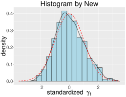
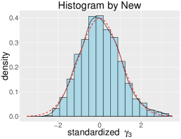
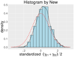
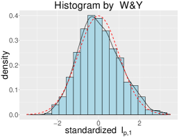
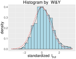
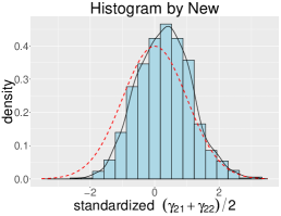
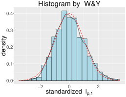
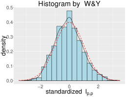
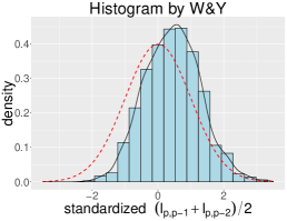
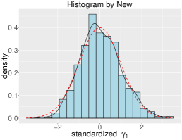
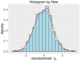
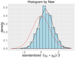
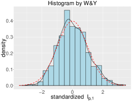
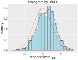
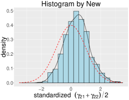
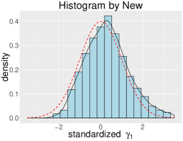
Table 1 depicts the nine typical percentiles of the empirical distributions of the standardized estimated eigenvalues, in which the $\psi_{n,k}$ and $\sigma_{k}^{2}$ were calculated by two methods: one is derived in Theorem 3.1, and the other one is derived in [33], to compare the finite sample properties of our method and Wang and Yao’s method [33]. The corresponding KS statistics of the two methods are also reported in Table 1. To see the overall pattern of the empirical distributions of the estimated spiked eigenvalues, we present their histograms based on 1000 simulations along with the kernel density estimate and asymptotic limiting distributions in Figures 1–3.

Figure 1 depicts the histograms and kernel density estimate of estimated eigenvalues when $x_{ij}$ and $y_{ij}$ follow $N(0,1)$. From Figure 1, we can see that under Gaussian population, both the empirical distributions of our method and Wang and Yao’s method are close to the asymptotical ones. This is further confirmed by the top panel of Table 1. The KS statistics of $\hat{\gamma}_{1}$ for Cases I and II and $\hat{\gamma}_{3}$ for Case II are very close for the two methods. Our newly proposed method has smaller KS statistics for $\hat{\gamma}_{2}^{*}$ for Cases I and II and $\hat{\gamma}_{3}$ for Case I than Wang and Yao’s method.

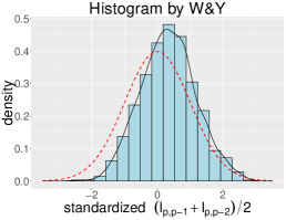
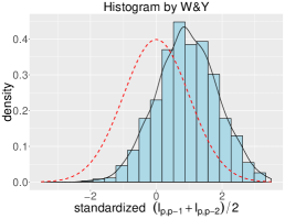
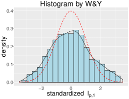
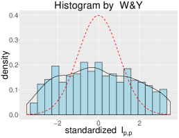
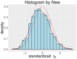
Figure 2 depicts the histograms and kernel density estimate of estimated eigenvalues when $P(x_{ij}=\pm 1)=P(y_{ij}\pm 1)=1/2$. Figure 2 clearly indicates that our method works well for both Case I and II, while Wang and Yao’s method works well for Case I, but not for Case II. The middle panel of Table 1 also delivers the same message. Except for $\hat{\gamma}_{1}$ in Case I, our method has much smaller KS statistics than Wang and Yao’s method. For the percentiles, it seems that Wang and Yao’s method has more spreading-out percentile. This implies it has larger variance.

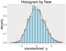
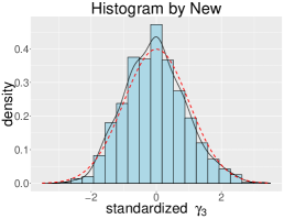
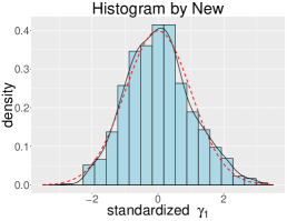
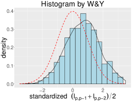
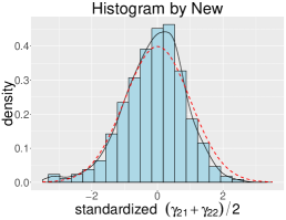
Figure 3 depicts the histograms and kernel density estimate of estimated eigenvalues when $x_{ij}$ and $y_{ij}$ follow $2^{-1/2}t(4)$. Figure 3 looks similar to the histograms for Case II in Figure 1. This implies that our method works well when the fourth moment of population distribution is unbounded. This can be further confirmed by comparing the bottom panel of Table 1 and the corresponding ones in the top panel of Table 1.

Table 2: Empirical sizes and powers

		$q_{1}/q_{0}=0.2$				$q_{1}/q_{0}=0.8$
		Size		Power		Size		Power
	$p$	New	CLRT	New	CLRT	New	CLRT	New	CLRT
$\tilde{c}_{1}=5,\tilde{c}_{2}=0.8$;	50	0.053	0.058	0.815	0.632	0.054	0.069	0.985	0.794
	100	0.043	0.053	1	0.935	0.051	0.046	1	0.899
	200	0.048	N.A.	1	N.A.	0.051	N.A.	1	N.A.
$\tilde{c}_{1}=5,\tilde{c}_{2}=0.5$;	50	0.043	0.057	1	0.998	0.051	0.049	1	1
	100	0.047	0.058	1	1	0.040	0.059	1	1
	200	0.039	N.A.	1	N.A.	0.044	N.A.	1	N.A.
$\tilde{c}_{1}=5,\tilde{c}_{2}=0.2$;	50	0.034	0.044	1	1	0.030	0.055	1	1
	100	0.038	0.049	1	1	0.043	0.052	1	1
	200	0.030	N.A.	1	N.A.	0.042	N.A.	1	N.A.
$\tilde{c}_{1}=2,\tilde{c}_{2}=0.8$;	50	0.042	0.056	0.547	0.467	0.051	0.058	0.838	0.598
	100	0.041	0.043	0.998	0.680	0.052	0.058	1	0.752
	200	0.057	N.A.	1	N.A.	0.055	N.A.	1	N.A.
$\tilde{c}_{1}=2,\tilde{c}_{2}=0.5$;	50	0.035	0.053	0.996	0.803	0.042	0.048	1	0.988
	100	0.052	0.056	1	0.995	0.041	0.052	1	1
	200	0.050	N.A.	1	N.A.	0.031	N.A.	1	N.A.
$\tilde{c}_{1}=2,\tilde{c}_{2}=0.2$;	50	0.041	0.062	1	1	0.041	0.046	1	1
	100	0.038	0.068	1	1	0.043	0.038	1	1
	200	0.047	N.A.	1	N.A.	0.038	N.A.	1	N.A.
$\tilde{c}_{1}=0.5,\tilde{c}_{2}=0.8$;	50	0.046	0.047	0.278	0.386	0.045	0.049	0.295	0.371
	100	0.055	0.049	1	0.658	0.058	0.054	0.957	0.574
	200	0.048	N.A.	1	N.A.	0.043	N.A.	1	N.A.
$\tilde{c}_{1}=0.5,\tilde{c}_{2}=0.5$;	50	0.047	0.048	1	0.699	0.045	0.043	1	0.785
	100	0.031	0.036	1	0.940	0.044	0.055	1	0.927
	200	0.051	N.A.	1	N.A.	0.048	N.A.	1	N.A.
$\tilde{c}_{1}=0.5,\tilde{c}_{2}=0.2$;	50	0.039	0.049	1	1	0.045	0.044	1	1
	100	0.037	0.047	1	1	0.044	0.053	1	1
	200	0.040	N.A.	1	N.A.	0.043	N.A.	1	N.A.

5.2 Numerical for Section 4

In this section, we conduct numerical study to compare the newly proposed test procedure for (17) in Section 4 with the corrected likelihood ratio test (CLRT) proposed by [4]. The simulation results for signal detections in Section 4.2 are similar to those for (17), we opt to omit them here to save space.

For testing hypothesis (17), we generate the elements of ${\bf B}_{2}$ be from $\mathcal{N}(1,1)$ for each simulation. Under the null hypothesis, we set ${\bf B}_{1}={\bf 0}$, while under the alternative hypothesis, half of the entries in the first column of ${\bf B}_{1}$ were generated from $\mathcal{N}(0.5,1)$ and the rest are zeros. Assume that the errors ${\boldsymbol{\varepsilon}}_{i}$ in (16) follows $\mathcal{N}_{p}(0,{\bf I}_{p})$. All elements of ${\bf z}_{i}$ in the model are independent and identically distributed and are sampled from $\mathcal{N}(1,0.5)$.

We consider two cases: $q_{1}/q_{0}=0.8$ and $q_{1}/q_{0}=0.2$. For each case, set $p=50,100,200$, $\tilde{c}_{1}=0.5,2,5$ and $\tilde{c}_{2}=0.2,0.5,0.8$. The limiting null distribution of Roy’s test $\lambda_{1}({\bf H}{\bf G}^{-1})$ follows the Tracy-Widom law for $\tilde{c}_{1}/\tilde{c}_{2}\lambda_{1}$ proposed by [17]. In order to avoid the calculation of the complex integral in the Tracy-Widom law, we derive the explicit expressions of the Tracy Widom law for $\tilde{c}_{1}/\tilde{c}_{2}\lambda_{1}$ by Theorem 1.12 in [3] based on the functional relationship of canonical correlation matrix and Fisher matrix. Then we report both empirical sizes and powers with 1000 replications at a significance level $\alpha=0.05$. The simulation results are summarized in the Tables 2.

The simulation illustrates that the limiting distribution of the Roy test in the linear regression model provides good sizes and powers in our simulation settings. Table 2 shows that the Roy’s test in this simulation setting seems to be more powerful than the CLRT. As seen from Table 2, the powers of the Roy test rapidly increases to 1 as the sample size increase. For instance, for the case of $q_{1}/q_{0}=0.2,p=50,\tilde{c}_{1}=2,\tilde{c}_{2}=0.8$ (i.e., $p=50,n=187,q_{0}=125,q_{1}=25$), the power is 0.547 and increases to 0.996 for the case of $q_{1}/q_{0}=0.2,p=50,\tilde{c}_{1}=2,\tilde{c}_{2}=0.5$ (i.e., $p=50,n=225,q_{0}=125,q_{1}=25$). In general, both the Roy’s test and the CLRT are expected to have good sizes, but our approach has higher powers in most cases. It is worth to noting that the CLRT cannot obtain the sizes and powers in the large-dimensional setting, since the log-likelihood ratio involved in the test statistic is approaching infinity for such cases. The limiting distribution derived in Section 4 can still be used to calculate the empirical powers even with the increasing dimension, while the CLRT fails when $p=200$.

The first author was supported by NSFC Grant 11971371 and Natural Science Foundation of Shaanxi Province 2020JM-049.

References

- Anderson [2003] Anderson,T. W. (2003). An introduction to Multivariate Statistical Analysis. 3rd ed. Wiley New York.
- Baik et al. [2005] Baik, J., Arous, G. B. & Pch, S. (2005). Phase transition of the largest eigenvalue for nonnull complex sample covariance matrices. The Annals of Probability, 33, 1643–1697.
- Bao et al. [2018] Bao, Z. G., Hu, J., Pan, G. M. & Zhou,W. (2018). Canonical correlation coefficients of high-dimensional Gaussian vectors: Finite rank case. The Annals of Statistics, 47, 612–640.
- Bai et al. [2013] Bai, Z. D., Jiang, D.D., Yao, J. F. & Zheng, S.R. (2013). Testing linear hypotheses in high-dimensional regressions. Statistics: A Journal of Theoretical and Applied Statistics, 47(6), 1207–1223.
- Bai, et al. [1991] Bai, Z.D., Miao, B.Q. and Rao, C. Radbakrisbna. (1991). Estimation of directions of arrival of signals: Asymptotic results. Advances in Spectrum Analysis and Array Processing, I, 327-347.
- Bai and Ng [2002] Bai, J. and Ng, S. (2002). Determining the number of factors in approximate factor models. Econometrica, 70, 191–221.
- Baik and Silverstein [2006] Baik, J. and Silverstein, J. W. (2006). Eigenvalues of large sample covariance matrices of spiked population models. Journal of Multivariate Analysis, 97, 1382–1408.
- Bai and Silverstein [1998] Bai, Z. D. and Silverstein, J.W. (1998). No eigenvalues outside the support of the limiting spectral distribution of large-dimensional sample covariance matrices. The Annals of Probability, 26, 316–345.
- Bai and Silverstein [2004] Bai, Z. D. and Silverstein, J.W. (2004). CLT for linear spectral statistics of large-dimensional sample covariance matrices. The Annals of Probability, 32, 553–605.
- Bai and Silverstein [2010] Bai, Z. D. and Silverstein, J.W. (2010). Spectral Analysis of Large Dimensional Random Matrices. Springer Series in Statistics, Springer-Verlag, New York, ISSN: 0172–7397.
- Bai and Yao [2008] Bai, Z. D. and Yao, J. F. (2008). Central limit theorems for eigenvalues in a spiked population model. Annales de l’Institut Henri Poincar - Probabilits et Statistiques, 44, (3), 447–474.
- Bai and Yao [2012] Bai, Z. D. and Yao, J. F. (2012). On sample eigenvalues in a generalized spiked population model. Journal of Multivariate Analysis, 106, 167–177.
- Bai and Zhou [2008] Bai, Z. D. and Zhou, W. (2008). Large sample covariance matrices without independence structures in columns. Statist. Sinica, 18, 425–442. MR2411613.
- Cai et al. [2020] Cai, T. T., Han, X. & Pan, G. M. (2020). Limiting Laws for Divergent Spiked Eigenvalues and Largest Non-spiked Eigenvalue of Sample Covariance Matrices. The Annals of Statistics, 48(3), 1255–1280.
- Fan and Wang [2017] Fan, J. and Wang, W. (2017). Asymptotics of Empirical Eigen-structure for Ultra-high Dimensional Spiked Covariance Model. The Annals of Statistics, 45(3), 1342–1374.
- Hu and Bai [2014] Hu, J. and Bai, Z.D. (2014). Estimation of directions of arrival of signals: Asymptotic results. Science China Mathematics, 57(11), DOI: 10.1007/s11425-014-4855-6.
- Han et al. [2016] Han, X., Pan, G.M. & Zhang, B. (2016). The Tracy-Widom Law for the largest eigenvalue of the Type matrices. The Annals of Statistics, 44(4), 1564–1592.
- Jiang and Bai [2021] Jiang, D. and Bai, Z.D. (2021). Generalized Four Moment Theorem and an Application to CLT for Spiked Eigenvalues of Large-dimensional Covariance Matrices. Bernoulli, 27(1), 274–294.
- Jiang et al. [2019] Jiang, D., Hu, J. & Hou, Z. Q. (2019). The limits of the sample spiked eigenvalues for a high-dimensional generalized Fisher matrix and its applications. arXiv:1912.02819v1.
- James [1964] James, A. T. (1964). Distributions of matrix variates and latent roots derived from normal samples. Annals of Mathematical Statistics, 35, 475–501.
- Johnstone [2001] Johnstone, I. (2001). On the distribution of the largest eigenvalue in principal components analysis. The Annals of Statistics, 29, 295–327.
- Johnstone and Nadler [2017] Johnstone, I. M.& B. Nadler, B. (2017). Roy’s largest root test under rank-one alternatives. Biometrika. 104(1), 181-193.
- Johnstone and Onatski [2020] Johnstone, I. M. and Onatski, A. (2020). Testing in High-dimensional Spiked Models. The Annals of Statistics, 48(3), 1231–1254.
- Onatski [2009] Onatski, A. (2009). Testing hypotheses about the number of factors in large factor models. Econometrica, 77, 1447–1479.
- Onatski [2012] Onatski, A. (2012). Asymptotics of the principal components estimator of large factor models with weakly influential factors. Journal of Econometrics, 168, 244–258.
- Paul [2007] Paul, D. (2007). Asymptotics of sample eigenstructure for a large dimensional spiked covariance model. Statistica Sinica, 17, 1617–1642.
- Levanon [1988] Levanon, N. (1988). Radar Principles. Wiley, New York.
- NS [2010] Nadakuditi, R. R. & Silverstein, J. W. Fundamental limit of sample generalized eigenvalue based detection of signals in noise using relatively few signal-bearing and noise only samples. IEEE J. Sel. Top. Signal Process, 4 468-480.
- Roy [1945] Roy, S. N. (1945). The individual sampling distribution of the maximum, the minimum and any intermediate of the -statistics on the null-hypothesis. Sankhy, 7, 133-158.
- Roy [1953] Roy, S. N. (1953). On a heuristic method of test construction and its use in multivariate analysis. Annals of Mathematical Statistics, 24, 220-238.
- Skorokhod [1956] Skorokhod, A. V. (1956). Limit theorems for stochastic processes. Theory Probab Appl., 1, 261-290.
- Wilks [1935] Wilks, S. S. (1935). On the independence of sets of normally distributed statistical variates. Econometrica, 3, 309–326.
- Wang and Yao [2017] Wang, Q. & Yao, J. F. (2017). Extreme eigenvalues of large-dimensional spiked fisher matrices with application. Annals of Statistics, 45(1), 415–445.
- Zeng and Liang [2009] Zeng, Y. H. & Liang, Y. C. (2009). Eigenvalue-based spectrum sensing algorithms for cognitive radio. IEEE Transactions Communications 57 1784-1793.
- Zheng et al. [2017] Zheng, S.R., Bai, Z.D. & Yao, J. F. (2017). CLT for eigenvalue statistics of large dimensional general Fisher matrices with applications. Bernoulli, 23(2), 1130–1178.