Markov partitions for the geodesic flow on compact Riemann surfaces of constant negative curvature

Abstract

It is well-known that hyperbolic flows admit Markov partitions of arbitrarily small size. However, the constructions of Markov partitions for general hyperbolic flows are very abstract and not easy to understand. To establish a more detailed understanding of Markov partitions, in this paper we consider the geodesic flow on Riemann surfaces of constant negative curvature. We provide a rigorous construction of Markov partitions for this hyperbolic flow with explicit forms of rectangles and local cross sections. The local product structure is also calculated in detail.

Keywords: Markov partitions; Symbolic dynamics; Geodesic flows; Constant negative curvatures

2020 MSC: 37B10, 37D40, 37D20, 57K32

1 Introduction

Symbolic dynamics has had a great history development and is a very useful method to study general dynamical systems. Instead of working on general dynamical systems, one can consider respective symbolic systems via symbolic dynamics. The symbolic dynamics of a dynamical system is constructed from Markov partitions, which have been attracting a lot of mathematicians. In 1967, a Markov partition for hyperbolic diffeomorphisms on 2-torus was constructed by Adler and Weiss in [1]. Then Sinai [24, 25] used successive approximations to construct a Markov partition for arbitrary $C$-diffeomorphisms. Bowen [4] used Sinai’s method to give a construction of Markov partitions for Smale’s Axiom A diffeomorphisms with the help of Smale’s Spectral Decomposition Theorem in [26]. In the case of $C$-flows on three-dimensional manifolds, a construction of Markov partitions was given by Ratner [21]. The author also introduced a Markov partition for transitive Anosov flows (so-called $C$-flows) on $n$-dimensional manifolds [22]. In 1973, Bowen modified and generalized the construction in [4] to have a Markov partition for $C^{1}$-hyperbolic flows in [6], which has become a classic reference. Pollicott [14] then constructed symbolic dynamics for Smale flows, which is a class of continuous flows on metric spaces provided a local product structure. The result generalizes Bowen’s construction of symbolic dynamics for $C^{1}$-hyperbolic flows in [6]. The problem is that all the constructions of Markov partitions mentioned above are very abstract and not easy to understand.

Pollicott and Sharp have found symbolic dynamics very useful in counting closed orbits for hyperbolic flows [19] and presenting asymptotic estimates for pairs of closed geodesics whose length differences lie in a prescribed family of shrinking intervals [18]; see also [16, 17] for other applications. Under supervision of Knieper, Bieder in his PhD thesis [3] used symbolic dynamics to construct partner orbits for hyperbolic flows. The purpose of construction of symbolic dynamics is to prove that a hyperbolic flow is semi-conjugated to a hyperbolic symbolic flow, in which the symbolic dynamics must be constructed from a Markov partition. A Markov partition is family of rectangles satisfying the Markov property. Then one can associate to a hyperbolic flow a mixing subshift of finite type $\sigma:\Lambda\rightarrow\Lambda$ and a Hölder continuous function $r:\Lambda\rightarrow\mathbb{R}$ such that, with at most a finite number of exceptions, the prime periodic orbit $\{x,\sigma x,...,\sigma^{k-1}x\}$ corresponds to the prime periodic orbit $\gamma$ whose word length and length are given by $|\gamma|=k$ and $l_{\gamma}=r^{k}(x)=r(x)+r(\sigma x)+\cdots+r(\sigma^{k-1}x)$, respectively; where $\Lambda=\{x=(x_{n})_{n=-\infty}^{\infty}:A(x_{n},x_{n+1})=1,\forall n\in{\mathbb{Z}}\}$, $A$ is the corresponding adjacency matrix with entries 0 or 1 of the Markov partition and $x_{n}$ are the symbols of rectangles in the Markov partition. Thus instead of working on the original hyperbolic flow, this viewpoint offers several advantages.

The main tool for the construction of the hyperbolic symbolic flow is the existence of a Markov partition for a basic set. However, for general hyperbolic flows, Markov partitions are not explicit and their constructions are not easy to understand as mentioned above. For instance, there are several results in [6] which need to be carefully verified. To establish a more detailed understanding of Markov partitions, in this paper we consider a concrete hyperbolic dynamical system, namely the geodesic flow on compact Riemann surfaces of constant negative curvature. We introduce explicit forms of rectangles as well as local cross sections. This leads to a more explicit and intuitive Markov partition for the system. Coordinalization of Poincaré sections helps us calculate the local product structure in detail and prove the existence of a pre-Markov partition. Especially, we even could somewhat simplify [6], in that we do not need several of the lemmas in this work. In addition, all important results in [6] in relevant to Markov partitions are rigorously verified.

The paper is organized as follows. In the next section, we give an introduction to the theory of the geodesic flow on compact factors of the hyperbolic plane with auxiliary results that will be used in this paper. Section 3 studies local product structure of the flow with specific calculations. Section 4 presents explicit forms of local cross sections and rectangles. Expansivity of the flow is studied in Section 5. The final section provides a rigorous construction of Markov partitions for the flow.

2 The geodesic flow on compact factors of the hyperbolic plane

We consider the geodesic flow on compact Riemann surfaces of constant negative curvature. It is well-known that any compact orientable surface with a metric of constant negative curvature is isometric to a factor $\Gamma\backslash\mathbb{H}^{2}$, where $\mathbb{H}^{2}=\{z=x+iy\in{\mathbb{C}}:\,y>0\}$ is the hyperbolic plane endowed with the hyperbolic metric $ds^{2}=\frac{dx^{2}+dy^{2}}{y^{2}}$ and $\Gamma$ is a discrete subgroup of the projective Lie group ${\rm PSL}(2,\mathbb{R})={\rm SL}(2,\mathbb{R})/\{\pm E_{2}\}$; here ${\rm SL}(2,\mathbb{R})$ is the group of all real $2\times 2$ matrices with unity determinant, and $E_{2}$ denotes the unit matrix. The group ${\rm PSL}(2,\mathbb{R})$ acts transitively on $\mathbb{H}^{2}$ by Möbius transformations $z\mapsto\frac{az+b}{cz+d}$. If the action is free (of fixed points), then the factor $\Gamma\backslash\mathbb{H}^{2}$ has a Riemann surface structure. Such a surface is a closed Riemann surface of genus at least $2$ and has the hyperbolic plane $\mathbb{H}^{2}$ as the universal covering. The geodesic flow $(\varphi_{t}^{\mathcal{X}})_{t\in\mathbb{R}}$ on the unit tangent bundle $\mathcal{X}=T^{1}(\Gamma\backslash\mathbb{H}^{2})$ goes along the unit speed geodesics on $\Gamma\backslash\mathbb{H}^{2}$.

On the other hand, the unit tangent bundle $T^{1}(\Gamma\backslash\mathbb{H}^{2})$ is isometric to the quotient space $\Gamma\backslash{\rm PSL}(2,\mathbb{R})=\{\Gamma g,g\in{\rm PSL}(2,\mathbb{R})\}$, which is the system of right co-sets of $\Gamma$ in ${\rm PSL}(2,\mathbb{R})$, by an isometry $\Xi$. Then the geodesic flow $(\varphi_{t}^{\mathcal{X}})_{t\in\mathbb{R}}$ can be equivalently described as the natural ‘quotient flow’

$$\varphi^{X}_{t}(\Gamma g)=\Gamma ga_{t}$$ (2.1)

on $X=\Gamma\backslash{\rm PSL}(2,\mathbb{R})$ associated to the flow $\phi_{t}(g)=ga_{t}$ on ${\rm PSL}(2,\mathbb{R})$ by the conjugate relation

$$\varphi_{t}^{\mathcal{X}}=\Xi^{-1}\circ\varphi_{t}^{X}\circ\Xi\quad\mbox{for all}\quad t\in\mathbb{R}.$$

Here $a_{t}\in{\rm PSL}(2,\mathbb{R})$ denotes the equivalence class obtained from the matrix $A_{t}=\Big{(}{\scriptsize\begin{array}[]{cc}e^{t/2}&0\\ 0&e^{-t/2}\end{array}}\Big{)}\in{\rm SL}(2,\mathbb{R})$.

There are some more advantages to work on $X=\Gamma\backslash{\rm PSL}(2,\mathbb{R})$ rather than on $\mathcal{X}=T^{1}(\Gamma\backslash\mathbb{H}^{2})$. One can calculate explicitly the stable and unstable manifolds at a point $x$ to be

$$W^{s}_{X}(x)=\{\theta^{X}_{t}(x),t\in\mathbb{R}\}\quad\mbox{and}\quad W^{u}_{X}(x)=\{\eta^{X}_{t}(x),t\in\mathbb{R}\},$$ (2.2)

where $(\theta^{X}_{t})_{t\in\mathbb{R}}$ and $(\eta^{X}_{t})_{t\in\mathbb{R}}$ are the stable horocycle flow and unstable horocycle flow defined by $\theta^{X}_{t}(\Gamma g)=\Gamma gb_{t}$ and $\eta^{X}_{t}(\Gamma g)=\Gamma gc_{t}$; here $b_{t},c_{t}\in{\rm PSL}(2,\mathbb{R})$ denote the equivalence classes obtained from $B_{t}=\big{(}{\scriptsize\begin{array}[]{cc}1&t\\ 0&1\end{array}}\big{)},\ C_{t}=\big{(}{\scriptsize\begin{array}[]{cc}1&0\\ t&1\end{array}}\big{)}\in{\rm SL}(2,\mathbb{R})$. The flow $(\varphi^{X}_{t})_{t\in\mathbb{R}}$ is hyperbolic, that is, for every $x\in X$ there exists an orthogonal and $(\varphi_{t}^{X})_{t\in\mathbb{R}}$-stable splitting of the tangent space $T_{x}X$

$$T_{x}X=E^{0}(x)\oplus E^{s}(x)\oplus E^{u}(x)$$

such that the differential of the flow $(\varphi_{t}^{X})_{t\in\mathbb{R}}$ is uniformly expanding on $E^{u}(x)$, uniformly contracting on $E^{s}(x)$ and isometric on $E^{0}(x)={\rm span}\big{\{}\frac{d}{dt}\varphi_{t}^{X}(x)|_{t=0}\big{\}}$. One can choose

$$E^{s}(x)={\rm span}\Big{\{}\frac{d}{dt}\,\theta^{X}_{t}(x)\Big{|}_{t=0}\Big{\}}\quad\mbox{and}\quad E^{u}(x)={\rm span}\Big{\{}\frac{d}{dt}\,\eta^{X}_{t}(x)\Big{|}_{t=0}\Big{\}}.$$

General references for this section are [2, 8, 12], and these works may be consulted for the proofs to all results which are stated above. In what follows, we will drop the superscript $X$ from $(\varphi^{X}_{t})_{t\in\mathbb{R}},(\theta^{X}_{t})_{t\in\mathbb{R}},(\eta^{X}_{t})_{t\in\mathbb{R}}$ to simplify notation.

2.1 Distance on $\Gamma\backslash{\rm PSL}(2,\mathbb{R})$

Lemma 2.1.

There is a natural Riemannian metric on $\mathsf{G}={\rm PSL}(2,\mathbb{R})$ such that the induced metric function $d_{\mathsf{G}}$ is left-invariant under $\mathsf{G}$ and

$$d_{\mathsf{G}}(a_{t},e)=\frac{1}{\sqrt{2}}|t|,\quad d_{\mathsf{G}}(b_{t},e)\leq|t|,\quad d_{\mathsf{G}}(c_{t},e)\leq|t|\quad\mbox{for all}\quad t\in\mathbb{R},$$

where $e=\pi(E_{2})$ is the unity of $\mathsf{G}$.

See [8, Subsection 9.3] for more details.

We define a metric function $d_{X}$ on $X=\Gamma\backslash{\rm PSL}(2,\mathbb{R})$ by

$$d_{X}(x_{1},x_{2})=\inf_{\gamma_{1},\gamma_{2}\in\Gamma}d_{\mathsf{G}}(\gamma_{1}g_{1},\gamma_{2}g_{2})=\inf_{\gamma\in\Gamma}d_{\mathsf{G}}(g_{1},\gamma g_{2}),$$ (2.3)

where $x_{1}=\Gamma g_{1}$, $x_{2}=\Gamma g_{2}$. In fact, if $X$ is compact, one can prove that the infimum is a minimum:

$$d_{X}(x_{1},x_{2})=\min_{\gamma\in\Gamma}d_{\mathsf{G}}(g_{1},\gamma g_{2}).$$

Lemma 2.2.

For any $x\in X$ and $t,s\in\mathbb{R}$, one has

$$d_{X}(\varphi_{t}(x),\varphi_{s}(x))\leq\frac{1}{\sqrt{2}}|t-s|.$$

Proof.

Suppose $x=\Gamma g$ for some $g\in{\rm PSL}(2,\mathbb{R})$, then

$$d_{X}(\varphi_{t}(x),\varphi_{s}(x)) =d_{X}(\Gamma ga_{t},\Gamma ga_{s})\leq d_{\mathsf{G}}(ga_{t},ga_{s})$$

$$=d_{\mathsf{G}}(a_{t},a_{s})=d_{\mathsf{G}}(a_{t-s},e)=\frac{1}{\sqrt{2}}|t-s|.$$

∎

It is well-known that the Riemann surface $\Gamma\backslash\mathbb{H}^{2}$ is compact if and only if the quotient space $X=\Gamma\backslash{\rm PSL}(2,\mathbb{R})$ is compact. It is possible to derive a uniform lower bound on $d_{\mathsf{G}}(g,\gamma g)$ for $g\in{\rm PSL}(2,\mathbb{R})$ and $\gamma\in\Gamma\setminus\{e\}$.

Lemma 2.3.

If the space $X=\Gamma\backslash{\rm PSL}(2,\mathbb{R})$ is compact, then there exists $0<\sigma_{*}<1$ such that

$$d_{\mathsf{G}}(\gamma g,g)>\sigma_{*}\quad\mbox{for all}\quad\gamma\in\Gamma\setminus\{e\}.$$

The number $\sigma_{*}$ is called an injectivity radius. See [23, Lemma 1, p. 237] for a similar result on $\Gamma\backslash\mathbb{H}^{2}$.

2.2 Poincaré sections

Definition 2.4 (Poincaré section).

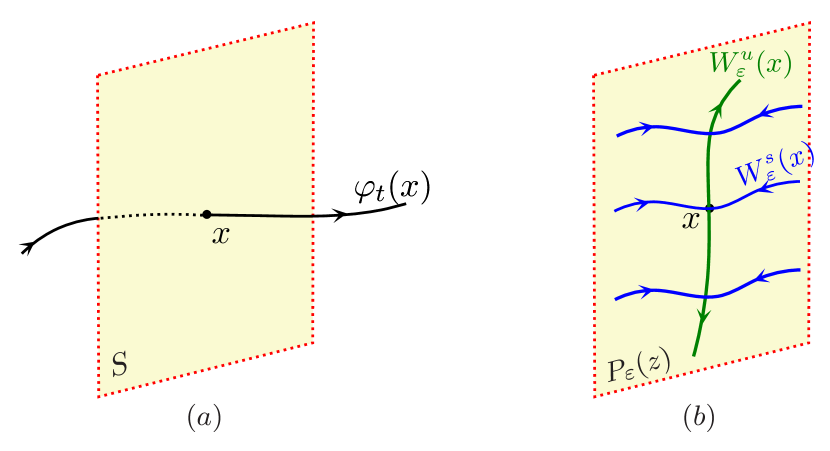
Let $x\in X$ and $\varepsilon>0$. The (closed) Poincaré section of radius $\varepsilon$ at $x$ is defined by

$$P_{\varepsilon}(x)=\{(\theta_{s}\circ\eta_{u})(x):|u|\leq\varepsilon,|s|\leq\varepsilon\}=\{\Gamma gc_{u}b_{s}:|u|\leq\varepsilon,|s|\leq\varepsilon\},$$

where $g\in\mathsf{G}$ is such that $x=\Gamma g$; see Figure 2 (a) for an illustration.

Another version of Poincaré section is

$$\widetilde{P}_{\varepsilon}(x)=\{(\eta_{u}\circ\theta_{s})(x):|u|\leq\varepsilon,|s|\leq\varepsilon\}=\{\Gamma gb_{s}c_{u}:|s|\leq\varepsilon,|u|\leq\varepsilon\}.$$

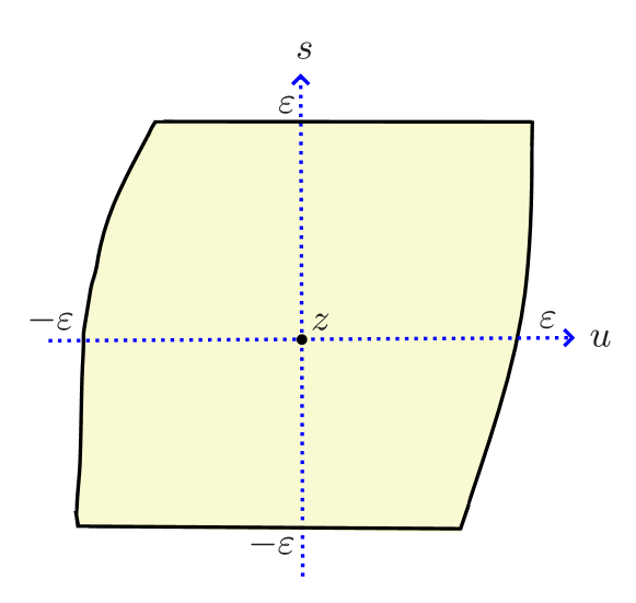
Note that both sets do not depend on the choice of $g\in\mathsf{G}$ such that $x=\Gamma g$. Similarly to open Poincaré sections in [9] one can coordinalize Poincaré sections in the case that the radius is small enough.

Lemma 2.5.

Let $X$ be compact, $\varepsilon\in\,(0,\sigma_{*}/4)$, and $x=\Gamma g$ for $g\in\mathsf{G}$.

(a) For every $y\in P_{\varepsilon}(x)$ there exists a unique couple $(u,s)\in\,[-\varepsilon,\varepsilon]\,\times\,[-\varepsilon,\varepsilon]$ such that $y=\Gamma gc_{u}b_{s}$. Then we write $y=(u,s)_{x}$.

(b) For every $y\in\widetilde{P}_{\varepsilon}(x)$ there exists a unique couple $(s,u)\in\,[-\varepsilon,\varepsilon]\,\times\,[-\varepsilon,\varepsilon]$ such that $y=\Gamma gb_{s}c_{u}$. Then we write $y=(s,u)^{\prime}_{x}$.

See [9, Lemma 2.1] for a proof.

2.3 Some auxiliary results

Lemma 2.6.

Let $g=[G]\in{\rm PSL}(2,\mathbb{R})$ for $G=\scriptsize\Big{(}\begin{array}[]{cc}a&b\\ c&d\end{array}\Big{)}\in{\rm SL}(2,\mathbb{R})$.

• If $a\neq 0$, then $g=c_{u}b_{s}a_{t}$ for

  $$t=2\ln|a|,\quad s=ab,\quad u=\frac{c}{a}.$$ (2.4)

• If $d\neq 0$, then $g=a_{t}b_{s}c_{u}$ for

  $$t=-2\ln|d|,\quad s={d},\quad u=\frac{c}{d}.$$

See [11, Lemma 2.3] for a proof of (a). A similar argument can be applied for (b).

Lemma 2.7.

For every $\varepsilon>0$ there is $\delta=\delta(\varepsilon)>0$ with the following property. If $g\in{\rm PSL}(2,\mathbb{R})$ is such that $d_{\mathsf{G}}(g,e)<\delta$, then there are

$$G=\Bigg{(}\begin{array}[]{cc}g_{11}&g_{12}\\ g_{21}&g_{22}\end{array}\Bigg{)}\in{\rm SL}(2,\mathbb{R})$$

satisfying $g=\pi(G)$ and $|g_{11}-1|+|g_{12}|+|g_{21}|+|g_{22}-1|<\varepsilon$.

See [11, Lemma 2.17] for a proof.

Lemma 2.8.

For every $\varepsilon>0$, there exists $\rho=\rho(\varepsilon)>0$ with the following property. For $x=\Gamma g$, $z=\Gamma gc_{u}b_{s}$ with $|s|,|u|<\sigma_{*}/8$ and $L>0$. Then

1. if $d_{X}(\varphi_{t}(x),\varphi_{t}(z))<3\rho$ for $t\in[-L,0]$, then $|s|<\varepsilon e^{-T}$;

2. if $d_{X}(\varphi_{t}(x),\varphi_{t}(z))<3\rho$ for $t\in[0,L]$, then $|u|<\varepsilon e^{-T}$.

See [9, Theorem 2.1] for a proof.

3 Local product structure

In this section we construct local product structure for the system. We use explicit forms of (local) stable and unstable manifolds to calculate local product structure in detail.

Definition 3.1.

Let $x\in X$ and $\varepsilon>0$. The local stable and local unstable manifold at $x$ are given by

$$W_{\varepsilon}^{s}(x)=\{\theta_{s}(x):|s|<\varepsilon\}=\{\Gamma gb_{s}:|s|<\varepsilon\}$$

and

$$W_{\varepsilon}^{u}(x)=\{\eta_{u}(x):|u|<\varepsilon\}=\{\Gamma gc_{u}:|u|<\varepsilon\}.$$

Note that both sets are independent of the choice of $g\in{\rm PSL}(2,\mathbb{R})$ such that $x=\Gamma g$. We also need the notion of local weak-stable and local weak-unstable manifold:

$$W^{ws}_{\varepsilon}(x)=\{\Gamma ga_{t}b_{s}:|t|<\varepsilon,|s|<\varepsilon\},$$

$$W^{wu}_{\varepsilon}(x)=\{\Gamma ga_{t}c_{u}:|t|<\varepsilon,|u|<\varepsilon\}.$$

Lemma 3.2.

Let $\varepsilon\in(0,\sigma_{*}/5)$. There exists a $\delta=\delta(\varepsilon)>0$ with the following property. If $x,y\in X$ satisfy $d_{X}(x,y)<\delta$, then the intersection

$$W^{ws}_{\varepsilon}(x)\cap W^{u}_{\varepsilon}(y)$$

consists of a unique point, and furthermore the intersection

$$W^{wu}_{\varepsilon}(x)\cap W^{s}_{\varepsilon}(y)$$

consists of a unique point.

Proof.

We prove the first assertion only. In order to show that such a $z\in W^{ws}_{\varepsilon}(x)\cap W^{u}_{\varepsilon}(y)$ does exist, note that according to Lemma 2.7 there is $\delta=\delta(\varepsilon)>0$ so that the following holds. If $u\in\mathsf{G}$ and $d_{\mathsf{G}}(u,e)<\delta$, then there is

$$A=\bigg{(}\begin{array}[]{cc}a&b\\ c&d\end{array}\bigg{)}\in{\rm SL}(2,\mathbb{R})$$ (3.5)

such that $u=\pi(A)$ and $|a-1|+|b|+|c|+|d-1|<\min\{\frac{1}{2},\frac{\varepsilon}{4}\}$. Fix $x,y\in X$ with $d_{X}(x,y)<\delta$. Let $g\in\mathsf{G}$ and $h\in\mathsf{G}$ satisfy $x=\Gamma g$ and $y=\Gamma h$ as well as $d_{X}(x,y)=d_{\mathsf{G}}(g,h)$. Then

$$d_{\mathsf{G}}(g^{-1}h,e)=d_{\mathsf{G}}(g,h)=d_{X}(x,y)<\delta,$$

and hence there is $A\in{\rm SL}(2,\mathbb{R})$ as in (3.5) such that $g^{-1}h=[A]$ and $|a-1|+|b|+|c|+|d-1|<\min\{\frac{1}{2},\frac{\varepsilon}{4}\}$; then in particular $d\in[1/2,3/2]$ holds. We can write $g^{-1}h=a_{t}b_{s}c_{u}$ for

$$t=-2\ln d,\quad s=bd,\quad u=\frac{c}{d}.$$

Then $hc_{-u}=ga_{t}b_{s}$ and also $|t|=2|\ln d|\leq 4|d-1|<\varepsilon$ due to $|\ln(1+z)|\leq 2|z|$ for $|z|\leq 1/2$. Furthermore, $|s|=|b||d|\leq 2|b|<\varepsilon/2$ and $|u|=\frac{|c|}{|d|}\leq 2|c|<\varepsilon/2$. Therefore if we put $z=\Gamma ga_{t}b_{s}=\Gamma hc_{-u}\in X$, then $z\in W^{ws}_{\varepsilon}(x)\cap W^{u}_{\varepsilon}(y)$. It remains to prove that the intersection point is unique. To establish this assertion, suppose that also $z^{\prime}\in W^{ws}_{\varepsilon}(x)\cap W^{u}_{\varepsilon}(y)$. Then $z^{\prime}=\Gamma ga_{t^{\prime}}b_{s^{\prime}}=\Gamma hc_{-u^{\prime}}$ for some $|t^{\prime}|,|s^{\prime}|,|u^{\prime}|<\varepsilon$. Hence $\Gamma hc_{u}a_{t}b_{s}=\Gamma g=\Gamma hc_{u^{\prime}}a_{t^{\prime}}b_{s^{\prime}}$, which means that $hc_{u}a_{t}b_{s}=\gamma hc_{u^{\prime}}a_{t^{\prime}}b_{s^{\prime}}$ for an appropriate element $\gamma\in\Gamma$. This yields

$$d_{\mathsf{G}}(\gamma hc_{u^{\prime}}a_{t^{\prime}}b_{s^{\prime}},hc_{u^{\prime}}a_{t^{\prime}}b_{s^{\prime}}) = d_{\mathsf{G}}(hc_{u}a_{t}b_{s},hc_{u^{\prime}}a_{t^{\prime}}b_{s^{\prime}})=d_{\mathsf{G}}(c_{u}a_{t}b_{s},c_{u^{\prime}}a_{t^{\prime}}b_{s^{\prime}})$$

$$\leq d_{\mathsf{G}}(c_{u}a_{t}b_{s},e)+d_{\mathsf{G}}(c_{u^{\prime}}a_{t^{\prime}}b_{s^{\prime}},e)$$

$$\leq |u|+\frac{1}{\sqrt{2}}|t|+|s|+|u^{\prime}|+\frac{1}{\sqrt{2}}|t^{\prime}|+|s^{\prime}|<5\varepsilon<\sigma_{*}.$$

From the property of $\sigma_{*}$ we deduce that $\gamma=e$ and therefore $c_{u}a_{t}b_{s}=c_{u^{\prime}}a_{t^{\prime}}b_{s^{\prime}}$. Multiplying out the matrices we obtain $u=u^{\prime}$, $t=t^{\prime}$, and $s=s^{\prime}$, and accordingly $z=\Gamma gb_{-s}=\Gamma gb_{-s^{\prime}}=z^{\prime}$. ∎

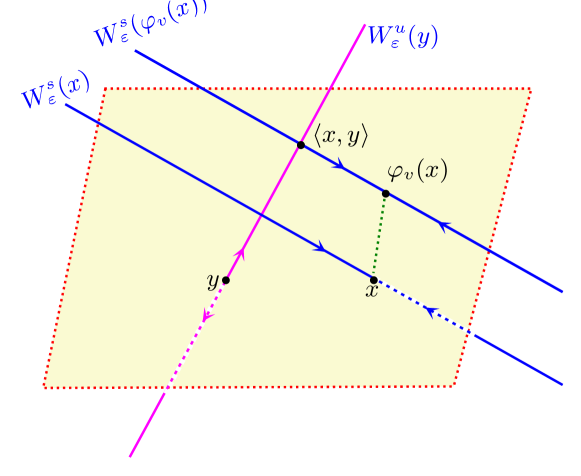
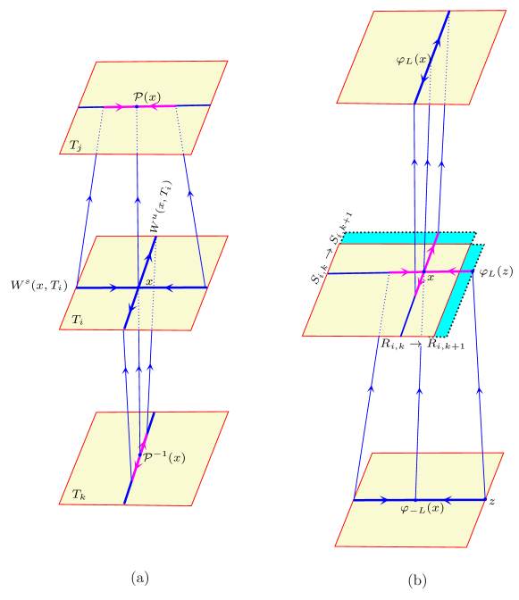
Corollary 3.3 (Local product structure).

Let $\varepsilon\in(0,\sigma_{*}/5)$. There exists a positive number $\delta=\delta(\varepsilon)$ with the following property. If $x,y\in X$ and $d_{X}(x,y)\leq\delta$, then there is a unique $v=v(x,y)\in\mathbb{R}$, $|v|\leq\varepsilon$ such that

$$W^{s}_{\varepsilon}(\varphi_{v}(x))\cap W^{u}_{\varepsilon}(y)\neq\varnothing.$$

More precisely, the intersection is a single point, denoted by $\langle x,y\rangle$. Furthermore, the map $\langle\cdot,\cdot\rangle$ is continuous on $\{(x,y)\in X\times X:d_{X}(x,y)<\delta\}.$

Proof.

Let $\varepsilon\in(0,\sigma_{*}/5)$ and let $\delta=\delta(\varepsilon)$ be as in Lemma 3.2. Let $x,y\in X$ be such that $d_{X}(x,y)<\delta$. Then $W^{ws}_{\varepsilon}(x)\cap W^{u}_{\varepsilon}(y)\neq\varnothing$, i.e., if $x=\Gamma g$ and $y=\Gamma h$, then there are $s,v,u\in(-\varepsilon,\varepsilon)$ such that $\Gamma ga_{v}b_{s}=\Gamma hc_{u}$. Since $\varphi_{v}(x)=\Gamma ga_{v}$ we have

$$W^{s}_{\varepsilon}(\varphi_{v}(x))=\{\Gamma ga_{v}b_{s^{\prime}}:|s^{\prime}|<\varepsilon\},$$

and hence $\Gamma ga_{t}b_{s}=\Gamma hc_{u}\in W^{s}_{\varepsilon}(\varphi_{v}(x))\cap W^{u}_{\varepsilon}(y)$. If also $W^{s}_{\varepsilon}(\varphi_{v^{\prime}}(x))\cap W^{u}_{\varepsilon}(y)\neq\varnothing$ for some $|v^{\prime}|<\varepsilon$, then $\Gamma ga_{v^{\prime}}b_{s^{\prime}}=\Gamma hc_{u^{\prime}}$ for appropriate $|s^{\prime}|,|u^{\prime}|<\varepsilon$. From Lemma 3.2 we obtain $v=v^{\prime}$, $s=s^{\prime}$, and $u=u^{\prime}$, so that $v$ is unique. That the intersection is a single point also follows from Lemma 3.2; see Figure 1 for an illustration. The last assertion is obvious. ∎

Figure 1: Local product structure

Fix $\varepsilon\in(0,\sigma_{*}/5)$ and let $\delta_{1}=\delta(\varepsilon)$ from Corollary 3.3 above. Define $\delta_{2}=\min\{\delta(\frac{\delta_{1}}{3}),\frac{\delta_{1}}{3}\}$. We also have a similar result to [4, Lemma 6].

Lemma 3.4.

Let $x,y,z,w\in X$ be such that ${\rm diam\,}\{x,y,z,w\}<\delta_{2}$. Then

(a) $\langle\langle x,y\rangle,z\rangle=\langle x,\langle y,z\rangle\rangle=\langle x,z\rangle$;

(b) $\langle\langle x,y\rangle,\langle z,w\rangle\rangle=\langle x,w\rangle$.

Proof.

For $x,y,z,w\in X$, we first check that all the notations make sense if ${\rm diam\,}\{x,y,z,w\}<\delta_{2}$. Obviously $\langle a,b\rangle$ makes sense for all $a,b\in\{x,y,z,w\}$. Write $y=\Gamma g$ and $w=\Gamma h$ for $g,h\in{\rm PSL}(2,\mathbb{R})$. By the proof of Lemma 3.2, $\langle x,y\rangle=\Gamma gc_{u_{1}}$ for some $|u_{1}|<\delta_{1}/3$ and $\langle z,w\rangle=\Gamma hc_{u_{2}}$ for some $|u_{2}|<\delta_{1}/3$. Then

$$d_{X}(\langle x,y\rangle,z) =d_{X}(\Gamma gc_{u_{1}},z)\leq d_{X}(\Gamma gc_{u_{1}},\Gamma g)+d_{X}(y,z)$$

$$\leq|u_{1}|+d_{X}(y,z)<\delta_{1}/3+\delta_{1}/3<\delta_{1}$$

so $\langle\langle x,y\rangle,z\rangle$ makes sense. Similarly, $\langle x,\langle y,z\rangle\rangle$ also makes sense. Next,

$$d_{X}(\langle x,y\rangle,\langle z,w\rangle) =d_{X}(\Gamma gc_{u_{1}},\Gamma hc_{u_{2}})\leq d_{X}(\Gamma gc_{u_{1}},\Gamma g)+d_{X}(y,w)+d_{X}(\Gamma h,\Gamma hc_{u_{2}})$$

$$<|u_{1}|+\delta_{1}/3+|u_{2}|<\delta_{1}$$

and hence $\langle\langle x,y\rangle,\langle z,w\rangle\rangle$ also makes sense.

(a) Note that if $x^{\prime}\in W^{ws}_{\frac{\delta_{1}}{3}}(x)$, then $W^{ws}_{\frac{\delta_{1}}{3}}(x^{\prime})\subset W^{ws}_{\delta_{1}}(x)$ and if $z^{\prime}\in W^{u}_{\frac{\delta_{1}}{3}}(z)$, then $W^{u}_{\frac{\delta_{1}}{3}}(z^{\prime})\subset W^{u}_{\frac{2\delta_{1}}{3}}(z)$. By Lemma 3.2, $\langle x,y\rangle\in W^{ws}_{\frac{\delta_{1}}{3}}(x)$ and

$$\langle\langle x,y\rangle,z\rangle\in W^{ws}_{\frac{\delta_{1}}{3}}(\langle x,y\rangle)\cap W^{u}_{\frac{\delta_{1}}{3}}(z)\in W^{ws}_{\delta_{1}}(x)\cap W^{u}_{\delta_{1}}(z)=\langle x,z\rangle.$$

Similarly, $\langle y,z\rangle\in W^{u}_{\varepsilon}(z)$ implies

$$\langle x,\langle y,z\rangle\rangle\in W^{ws}_{\frac{\delta_{1}}{3}}(x)\cap W^{u}_{\frac{\delta_{1}}{3}}(\langle y,z\rangle)\in W^{ws}_{\frac{\delta_{1}}{3}}(x)\cap W^{u}_{\frac{2\delta_{1}}{3}}(z)=\langle x,z\rangle.$$

(b) Applying (a), we have $\langle\langle x,y\rangle,\langle z,w\rangle\rangle=\langle\langle x,y\rangle,w\rangle=\langle x,w\rangle$. ∎

4 Local cross sections and rectangles

This section deals with rectangles included in Poincaré sections. We introduce explicit forms of rectangles that leads to more explicit Markov partition afterwards.

4.1 Local cross sections

Definition 4.1 (Local cross section).

A set $S\subset X$ is called a cross section of time $\varepsilon>0$ for the flow $(\varphi_{t})_{t\in\mathbb{R}}$ if

1. $S$ is closed;

2. $S\cap\varphi_{[-\varepsilon,\varepsilon]}(x)=\{x\}$ for all $x\in S$.

See Figure 2 (a) for an illustration.

Figure 2: (a) Local cross section,  (b) Poincaré section

We consider an example of local cross sections.

Lemma 4.2.

Let $\varepsilon>0,\alpha>0$ be such that $4\varepsilon+2\alpha<\sigma_{*}$ and let $z=\Gamma g\in X$. The closed Poincaré sections

$$P_{\varepsilon}(z) =\{\Gamma gc_{u}b_{s},\ |u|\leq\varepsilon,|s|\leq\varepsilon\}$$

$$\widetilde{P}_{\varepsilon}(z) =\{\Gamma gb_{s}c_{u},\ |s|\leq\varepsilon,|u|\leq\varepsilon\}$$

are local cross sections of time $\alpha$ and with diameters at most $4\varepsilon$.

Proof.

Obviously, $P_{\varepsilon}(z)$ is closed. Note that

$${\mathcal{Q}}:=\varphi_{[-\varepsilon,\varepsilon]}(P_{\varepsilon}(z))=\{\Gamma gc_{u}b_{s}a_{t},|u|\leq\varepsilon,|s|\leq\varepsilon,|t|\leq\alpha\}.$$

In order to verify Assumption (b), we check that every point $x\in{\mathcal{Q}}$ has a unique triple $(u,s,t)\in[-\varepsilon,\varepsilon]^{2}\times[-\alpha,\alpha]$ such that $x=\Gamma gc_{u}b_{s}a_{t}$. To show its uniqueness, suppose that $z=\Gamma g_{1}=\Gamma g_{2}$ and $x=\Gamma g_{1}b_{s_{1}}c_{u_{1}}a_{t_{1}}=\Gamma g_{2}b_{s_{2}}c_{u_{2}}a_{t_{2}}$ for $g_{1},g_{2}\in\mathsf{G}$ and $(u_{i},s_{i},t_{i})\in[-\varepsilon,\varepsilon]^{2}\times[-\alpha,\alpha]$. Then there are $\gamma,\gamma^{\prime}\in\Gamma$ such that

$$\gamma g_{1}=g_{2}\quad\mbox{and}\quad\gamma^{\prime}g_{1}c_{u_{1}}b_{s_{1}}a_{t_{1}}=g_{2}c_{u_{2}}b_{s_{2}}a_{t_{2}}.$$

Therefore,

$$d_{\mathsf{G}}(\gamma^{-1}\gamma^{\prime}g_{1}c_{u_{1}}b_{s_{1}},g_{1}c_{u_{1}}b_{s_{1}})$$

$$= d_{\mathsf{G}}(\gamma^{-1}g_{2}c_{u_{2}}b_{s_{2}}a_{t_{2}-t_{1}},g_{1}c_{1}b_{s_{1}})=d_{\mathsf{G}}(g_{1}c_{u_{2}}b_{s_{2}}a_{t_{2}-t_{1}},g_{1}c_{u_{1}}b_{s_{1}})$$

$$= d_{\mathsf{G}}(c_{u_{2}-u_{1}}b_{s_{2}}a_{t_{2}-t_{1}},b_{s_{1}})\leq d_{\mathsf{G}}(c_{u_{2}-u_{1}}b_{s_{2}}a_{t_{2}-t_{1}},e)+d_{\mathsf{G}}(b_{s_{1}},e)$$

$$\leq |u_{2}-u_{1}|+|s_{2}|+|t_{2}-t_{1}|+|s_{1}|<4\varepsilon+2\alpha<\sigma_{*}.$$

From the property of $\sigma_{*}$, this implies that $\gamma^{-1}\gamma^{\prime}=e$, so that $\gamma=\gamma^{\prime}$. Then $g_{2}c_{u_{2}}b_{s_{2}}a_{t_{2}}=\gamma g_{1}c_{u_{1}}b_{s_{1}}a_{t_{1}}=g_{2}c_{u_{1}}b_{s_{1}}a_{t_{1}}$ yields $c_{u_{1}}b_{s_{1}}a_{t_{1}}=c_{u_{2}}b_{s_{2}}a_{t_{2}}$, and consequently $u_{2}=u_{1},s_{2}=s_{1},t_{2}=t_{1}$ by considering matrices. This leads to $\varphi_{[-\alpha,\alpha]}(x)\cap P_{\varepsilon}(z)=\{x\}$ and hence $P_{\varepsilon}(z)$ is a local cross section of time $\varepsilon$. For the last assertion, if $x=\Gamma gc_{u_{x}}b_{s_{x}},y=\Gamma gc_{u_{y}}b_{s_{y}}\in P_{\varepsilon}(z)$, then

$$d_{X}(x,y)\leq d_{\mathsf{G}}(c_{u_{x}}b_{s_{x}},c_{u_{y}}b_{s_{y}})\leq|u_{x}|+|s_{x}|+|u_{y}|+|s_{y}|\leq 4\varepsilon$$

shows ${\rm diam\,}P_{\varepsilon}(z)\leq 4\varepsilon$. The same argument can be applied for $\widetilde{P}_{\varepsilon}(z)$. ∎

By the same manner as in the previous proof, it follows the next result.

Proposition 4.3.

(a) Let ${\tt u}>0,{\tt s}>0$ and $\alpha>0$ be such that $2{\tt u}+2{\tt s}+\alpha<\sigma_{*}$ and let $z=\Gamma g\in X$. The sets

$$P_{\tt s}^{\tt u}(z)=\{\Gamma gc_{u}b_{s},\ |u|\leq{\tt u},|s|\leq{\tt s}\},\ \widetilde{P}_{\tt u}^{\tt s}(z)=\{\Gamma gb_{s}c_{u},\ |s|\leq{\tt s},|u|\leq{\tt u}\}$$

are local cross sections of time $\alpha$ and with diameters at most $2({\tt u}+{\tt s})$.

(b) Let $\varepsilon>0,\alpha>0,\tau\in\mathbb{R}$ be such that $2\varepsilon(e^{\tau}+e^{-\tau})+\alpha<\sigma_{*}$ and let $z=\Gamma g\in X$. The sets

$$\varphi_{\tau}(P_{\varepsilon}(z))=\{\Gamma ga_{\tau}c_{ue^{\tau}}b_{se^{-\tau}}:|u|\leq\varepsilon,|s|\leq\varepsilon\}=P_{\varepsilon e^{-\tau}}^{\varepsilon e^{\tau}}(\varphi_{\tau}(z)),$$

$$\varphi_{\tau}(\widetilde{P}_{\varepsilon}(z))=\{\Gamma ga_{\tau}b_{se^{-\tau}}c_{ue^{\tau}}:|s|\leq\varepsilon,|u|\leq\varepsilon\}=\widetilde{P}_{\varepsilon e^{-\tau}}^{\varepsilon e^{\tau}}(\varphi_{\tau}(z))$$

are local cross sections of time $\alpha$ and with diameters at most $2\varepsilon(e^{\tau}+e^{-\tau})$.

For a general flow, the following result is not obvious, see [27]. However, for the geodesic flow on compact factors of the hyperbolic plane, it is quite simple.

Proposition 4.4.

For $x\in X$, there is a local cross section $S_{x}$ of time $\nu_{x}>0$ so that $x\in{\rm int\,}S_{x}$.

Proof.

We can choose $S_{x}=P_{\nu_{x}}(x)=\{\Gamma gc_{u}b_{s}:|s|,|u|\leq\nu_{x}\}$ for $\nu_{x}\in(0,\sigma_{*}/6)$; see Lemma 4.2. ∎

It is clear that if $S$ is a local cross section of time $\varepsilon$, then $S\times[-\alpha,\alpha]$ is homeomorphic with the compact set $\varphi_{[-\alpha,\alpha]}(S)$.

Definition 4.5 (Projection map).

Let $S$ be a local cross section of time $\alpha$. The map

$${\rm pr}_{S}:\varphi_{[-\alpha,\alpha]}(S)\to S,\quad{\rm pr}_{S}(\varphi_{t}(x))=x\quad\mbox{for all}\quad t\in[-\alpha,\alpha]$$

is called the projection map to $S$.

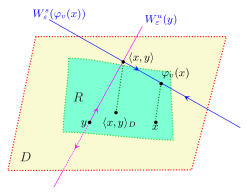
Let $\varepsilon\in(0,\sigma_{*}/6)$ and $\delta=\delta(\varepsilon)$ be as in Corollary 3.3. If $D$ is a local cross section of time $\varepsilon$ and $T\subset D$ is a closed set such that ${\rm diam\,}T<\delta$ and ${\rm diam\,}T$ and $d(T,\partial D)>0$. We assume that ${\rm pr}_{D}(\langle x,y\rangle)$ do exist for all $x,y\in T$. We define

$$\langle\cdot,\cdot\rangle_{D}:T\times T\longrightarrow D,\quad\langle x,y\rangle_{D}={\rm pr}_{D}(\langle x,y\rangle).$$ (4.6)

See Figure 3 for an illustration. It is worth mentioning that $\langle x,y\rangle_{D}\in D$ and may not be in $T$ and $\langle\cdot,\cdot\rangle_{D}:T\times T\to D$ is continuous.

From now on, we fix $\varepsilon\in(0,\sigma_{*}/5)$ and $\delta=\delta(\varepsilon)$ be from Corollary 3.3. The next result determines $\langle x,y\rangle_{D}$ precisely.

Lemma 4.6.

Let $D=P_{2\alpha}(z)$ and $T=P_{\alpha/4}(z)$ for $\alpha\in(0,\delta)$ and $z=\Gamma g\in X$. If $x=\Gamma gc_{u_{x}}b_{s_{x}},y=\Gamma gc_{u_{y}}b_{s_{y}}\in T$, then

$$\langle x,y\rangle=\Gamma gc_{u_{x}}b_{s_{x}+s}a_{v}=\Gamma hc_{u_{y}}b_{s_{y}}c_{u},\mbox{\ \ }\langle x,y\rangle_{D}=\Gamma gc_{u_{x}}b_{s_{w}}=\Gamma gc_{u_{y}}b_{s_{y}}c_{u}a_{-v}\in D,$$

where $s,u,v,s_{w}$ are defined by

$$s=(s_{y}-s_{x}-s_{x}s_{y}(u_{y}-u_{x}))(1+(u_{y}-u_{x})s_{y}),\quad u=\frac{u_{x}-u_{y}}{1+(u_{y}-u_{x})s_{y}},$$ (4.7)

$$v=-2\ln(1+(u_{y}-u_{x})s_{y}),\quad s_{w}=\frac{s_{y}}{1+(u_{y}-u_{x})s_{y}}.$$

Proof.

Since ${\rm diam\,}T\leq\alpha<\delta$, $\langle x,y\rangle$ do exist for all $x,y\in T$. First we have

$$B_{-s_{x}}C_{u_{y}-u_{x}}B_{s_{y}}=\begin{pmatrix}1-(u_{y}-x_{x})s_{y}&s_{x}-s_{x}-s_{x}s_{y}(u_{y}-u_{x})\\ u_{y}-u_{x}&1+(u_{y}-u_{x})s_{y}\end{pmatrix}$$

and $\pi(B_{-s_{x}}C_{u_{y}-u_{x}}B_{s_{y}})=b_{-s_{x}}c_{u_{y}-u_{x}}b_{s_{y}}=(c_{u_{x}}b_{s_{x}})^{-1}c_{u_{y}}b_{s_{y}}$. Let $s,u,v,s_{w}$ be defined by (4.7). Then $s,u,v,s_{w}\in[-\varepsilon,\varepsilon]$. By Lemma 2.6 (b), $b_{-s_{x}}c_{u_{y}-u_{x}}b_{s_{y}}=a_{v}b_{s}c_{-u}$. This implies $\Gamma gc_{u_{x}}b_{s_{x}}a_{v}b_{s}=\Gamma gc_{u_{y}}b_{s_{y}}c_{u}\in W^{s}_{\varepsilon}(\varphi_{v}(x))\cap W^{u}_{\varepsilon}(y)=\langle x,y\rangle$. Furthermore, $\langle x,y\rangle=\Gamma gc_{u_{x}}b_{s_{x}}s_{se^{v}}a_{v}=\Gamma gc_{u_{x}}b_{s_{w}}a_{v}$ after a short calculation. Consequently, $\varphi_{-v}(\langle x,y\rangle)=\Gamma gc_{u_{y}}b_{s_{y}}c_{u}a_{-v}=\Gamma gc_{u_{x}}b_{s_{w}}\in D$ yields $\langle x,y\rangle_{D}=\Gamma gc_{u_{x}}b_{s_{w}}=\Gamma gc_{u_{y}}b_{s_{y}}c_{u}a_{-v}$, proving the lemma. ∎

4.2 Rectangles

In this subsection, we fix $\varepsilon_{*}\in(0,\sigma_{*}/5)$ and $\delta_{*}=\delta(\varepsilon_{*})$ from Corollary 3.3.

It was mentioned in the last subsection that for a local cross section $D$ and $R\subset D$, if $x,y\in R$ then $\langle x,y\rangle_{D}$ may not be in $R$.

Definition 4.7 (Rectangle).

Let $D$ be a local cross section and ${\rm diam\,}D<\delta$. A subset $\varnothing\neq R\subset D$ is called a rectangle if

• $R$ is closed in $D$;

• $\langle x,y\rangle_{D}\in R$ for all $x,y\in R$.

See Figure 3 for an illustration. In the case that $R$ is a rectangle, for $x,y\in R$ we can write $\langle x,y\rangle_{R}$ for $\langle x,y\rangle_{D}$ since it does not depend on $D$.

Figure 3: Rectangle $R$ in local cross section $D$

Remark 4.8.

(a) If $R_{1}\subset D_{1}$ and $R_{2}\subset D_{2}$ are rectangles and $R_{1}\cap R_{2}\neq\varnothing$, then $R_{1}\cap R_{2}$ is a rectangle.

(b) If $R\subset D$ is a rectangle, then so is $\varphi_{\tau}(R)$ for appropriately small $\tau\in\mathbb{R}$. Indeed, assume that $x,y\in\varphi_{\tau}(R)$. Then $x=\varphi_{\tau}(x^{\prime})$ and $y=\varphi_{\tau}(y^{\prime})$ for $x^{\prime},y^{\prime}\in R$. Write $x^{\prime}=\Gamma g$ and $y^{\prime}=\Gamma h$. Assume that $\langle x^{\prime},y^{\prime}\rangle=\Gamma ga_{v}b_{s}=\Gamma hc_{u}$ for some small numbers $v,s,u\in\mathbb{R}$. Then $\langle x,y\rangle=\Gamma ga_{\tau}a_{v^{\prime}}b_{s^{\prime}}=\Gamma ha_{\tau}c_{u^{\prime}}$ with $v^{\prime}=v,s^{\prime}=se^{-\tau}$ and $u^{\prime}=ue^{\tau}$. This yields $\langle x,y\rangle=\Gamma ga_{v}b_{s}a_{\tau}=\varphi_{\tau}(\langle x^{\prime},y^{\prime}\rangle)$. If $\varphi_{\lambda}(\langle x^{\prime},y^{\prime}\rangle)=\langle x^{\prime},y^{\prime}\rangle_{R}\in\mathbb{R}$, then $\varphi_{\lambda}(\langle x,y\rangle)=\varphi_{\tau}(\varphi_{\lambda}(\langle x^{\prime},y^{\prime}\rangle))\in\varphi_{\tau}(R)$ implies that $\varphi_{\lambda}(\langle x,y\rangle)=\langle x,y\rangle_{\varphi_{\tau}(R)}\in\varphi_{\tau}(R)$. $\Diamond$

The next result gives us an explicit example of rectangles; see Figure 4 for an illustration.

Figure 4: Rectangle $S_{\varepsilon}(z)$

Proposition 4.9 (Rectangle).

Let $\varepsilon\in(0,1)$ be such that $\frac{\varepsilon}{1-\varepsilon^{2}}\in(0,\delta_{*}/4)$ and $z\in X$. The sets

$$S_{\varepsilon}(z) = \Big{\{}\Gamma gc_{u}b_{s}\,:\,u\in[-\varepsilon,\varepsilon],\,s=\frac{s^{\prime}}{1-us^{\prime}}\quad\mbox{for some}\quad s^{\prime}\in[-\varepsilon,\varepsilon]\Big{\}},$$

$$T_{\varepsilon}(z) = \Big{\{}\Gamma gb_{s}c_{u}\,:\,s\in[-\varepsilon,\varepsilon],\,u=\frac{u^{\prime}}{1-su^{\prime}}\quad\mbox{for some}\quad u^{\prime}\in[-\varepsilon,\varepsilon]\Big{\}}$$

are rectangles, where $g\in{\rm PSL}(2,\mathbb{R})$ is such that $z=\Gamma g$.

Proof.

We only prove for $S:=S_{\varepsilon}(z)\subset P_{2\varepsilon}(z)=:P$. Note that from the assumption, ${\rm diam\,}S<\delta_{2}$. Take $x=\Gamma gc_{u_{x}}b_{s_{x}},\ y=\Gamma gc_{u_{y}}b_{s_{y}}\in S$. Then $\langle x,y\rangle=W^{s}_{\varepsilon}(\varphi_{v}(x))\cap W^{u}_{\varepsilon}(y)=\Gamma gc_{u_{x}}b_{s_{x}}a_{v}b_{s}=\Gamma gc_{u_{y}}b_{s_{y}}c_{u}$ with

$$v=-2\ln(1+(u_{y}-u_{x})s_{y}),\ s =(s_{y}-s_{x}-(u_{y}-u_{x})s_{x}s_{y})(1+(u_{y}-u_{x})s_{y}),$$

$$u =\frac{u_{y}-u_{x}}{1+(u_{y}-u_{x})s_{y}}.$$

Rewriting $\langle x,y\rangle=\Gamma gc_{u_{x}}b_{s_{x}}a_{v}b_{s}=\Gamma gc_{u_{x}}b_{s_{x}+se^{v}}a_{v}$ implies that $\langle x,y\rangle_{P}=\Gamma gc_{u_{x}}b_{s_{x}+se^{v}}$. We need to verify $\Gamma gc_{u_{x}}b_{s_{x}+se^{v}}\in S$. A short calculation shows that $s_{x}+se^{v}=\frac{s_{y}}{1+(u_{y}-u_{x})s_{y}}=\frac{s_{y}^{\prime}}{1-u_{x}s_{y}^{\prime}}$, where $s_{y}^{\prime}\in[-\varepsilon,\varepsilon]$ satisfies $s_{y}=\frac{s_{y}^{\prime}}{1-u_{y}s_{y}^{\prime}}$; and thus $\langle x,y\rangle_{P}\in S$, which completes the proof. ∎

The following result is proved by the same manner as the previous theorem.

Proposition 4.10 (Rectangle).

Let ${\tt s},{\tt u}\in(0,1)$ be such that $\max\{\frac{\tt s}{1-{\tt su}},\frac{\tt u}{1-{\tt su}}\}<\delta_{*}/4$ and $z\in X$. The sets

$$S_{{\tt s}}^{{\tt u}}(z) = \Big{\{}\Gamma gc_{u}b_{s}\,:\,u\in[-{\tt u},{\tt u}],\,s=\frac{s^{\prime}}{1-us^{\prime}}\quad\mbox{for some}\quad s^{\prime}\in[-{\tt s},{\tt s}]\Big{\}},$$

$$T_{{\tt u}}^{{\tt s}}(z) = \Big{\{}\Gamma gb_{s}c_{u}\,:\,s\in[-{\tt s},{\tt s}],\,u=\frac{u^{\prime}}{1-su^{\prime}}\quad\mbox{for some}\quad u^{\prime}\in[-{\tt u},{\tt u}]\Big{\}}$$

are rectangles, where $g\in{\rm PSL}(2,\mathbb{R})$ such that $z=\Gamma g$.

Corollary 4.11.

Let $\varepsilon\in(0,1)$ and $\tau\in\mathbb{R}$ be such that $\frac{\varepsilon e^{|\tau|}}{1-\varepsilon^{2}}<\delta_{*}/4$. Then $\varphi_{\tau}(S_{\varepsilon}(z))$ and $\varphi_{\tau}(T_{\varepsilon}(z))$ are rectangles. More precisely, $\varphi_{\tau}(S_{\varepsilon}(z))=S_{\varepsilon e^{-\tau}}^{\varepsilon e^{\tau}}(z)$ whereas $\varphi_{\tau}(T_{\varepsilon}(z))=T_{\varepsilon e^{\tau}}^{\varepsilon e^{-\tau}}(z)$.

Remark 4.12.

It is easy to check that

$$S_{\varepsilon}(z)=\Big{\{}\Gamma gc_{u}b_{s}:u\in[-\varepsilon,\varepsilon],\,s\in\Big{[}\frac{-\varepsilon}{1+\varepsilon u},\frac{\varepsilon}{1+\varepsilon u}\Big{]}\Big{\}}\subset P_{\frac{\varepsilon}{1-\varepsilon^{2}}}(z).$$

Therefore, for a given local cross section $P_{\rho}(z)$, any rectangle $S_{\varepsilon}(z)$ with $\frac{\varepsilon}{1-\varepsilon^{2}}<\rho$ has the following property:

1. $S_{\varepsilon}(z)$ is closed and contained in $P_{\rho}(z)$;

2. ${\rm int\,}S_{\varepsilon}(z)=\big{\{}\Gamma gc_{u}b_{s}:s\in(-\varepsilon,\varepsilon),s=\frac{s^{\prime}}{1-us^{\prime}}\quad\mbox{for some}\quad s^{\prime}\in(-\varepsilon,\varepsilon)\big{\}}$.

Similar properties also hold for $T_{\varepsilon}(z)$. $\Diamond$

Each version of rectangles has its own special properties. In this paper we will use both of them. The following result is a relation between the two versions.

Lemma 4.13.

Let ${\tt u},{\tt s}\in(0,1)$ be such that $\max\{\frac{\tt s}{1-{\tt su}},\frac{\tt u}{1-{\tt su}}\}<\delta_{*}/4$ and $z\in X$. Let $S,T$ be local cross sections and let $S_{\tt s}^{\tt u}(z)\subset S,T_{\tt s}^{\tt u}(z)\subset T$ be rectangles defined in Proposition 4.9 such that ${\rm pr}_{T}(S_{\tt s}^{\tt u}(z))$ and ${\rm pr}_{S}(T_{\tt s}^{\tt u}(z))$ are well-defined. Then

$${\rm pr}_{T}(S_{\tt s}^{\tt u}(z))=T_{\tt u}^{\tt s}(z)\quad\mbox{and}\quad{\rm pr}_{S}(T_{\tt s}^{\tt u}(z))=S_{\tt u}^{\tt s}(z).$$ (4.8)

$S_{\tt s}^{\tt u}(z)$ is the projection of $T_{\tt s}^{\tt u}(z)$ on $S$ and $T_{\tt s}^{\tt u}(z)$ is the projection of $S_{\tt s}^{\tt u}(z)$ on $T$.

Proof.

For $x=\Gamma gc_{u}b_{s}\in S_{\tt s}^{\tt u}(z)$, we write $x=\Gamma gb_{\tilde{s}}c_{\tilde{u}}a_{\tilde{t}}$ for

$$\tilde{s}=\frac{s}{1+us},\quad\tilde{u}=u(1+us),\quad\tilde{t}=-2\ln(1+us).$$

By the definition of $S_{\tt s}^{\tt u}(z)$, $s=\frac{s^{\prime}}{1-us^{\prime}}$ for some $s^{\prime}\in[-{\tt s},{\tt s}]$. This implies that $\tilde{s}=s^{\prime}\in[-{\tt s},{\tt s}]$. In addition, $1-\tilde{s}u=1-\frac{s}{1+us}u=\frac{1}{1+us}$ yields $\tilde{u}=u(1+us)=\frac{u}{1-\tilde{s}u}$; hence $\tilde{x}=\varphi_{-\tilde{t}}(x)={\rm pr}_{T}(x)=\Gamma gb_{\tilde{s}}c_{\tilde{u}}\in T_{\tt u}^{\tt s}(z)$ shows that ${\rm pr}_{T}(S_{\tt s}^{\tt u}(z))\subset T_{\tt u}^{\tt s}(z)$. Conversely, if $\tilde{x}=\Gamma gb_{\tilde{s}}c_{\tilde{u}}\in T_{\tt u}^{\tt s}(z)$, then $\tilde{x}=\Gamma gc_{u}b_{s}a_{t}$ for

$$u=\frac{\tilde{u}}{1+\tilde{u}\tilde{s}},\quad s=\tilde{s}(1+\tilde{u}\tilde{s}),\quad t=2\ln(1+\tilde{u}\tilde{s}).$$

Similarly, we can check that $u\in[-{\tt u},{\tt u}]$ and $s=\frac{\tilde{s}}{1-u\tilde{s}}$ for $\tilde{s}\in[-{\tt s},{\tt s}]$. Set $x=\Gamma gc_{u}b_{s}\in S_{\tt s}^{\tt u}$ to get $x\in S_{\tt s}^{\tt u}$ and $\tilde{x}=\varphi_{t}(x)={\rm pr}_{T}(x)$, which verifies $T_{\tt u}^{\tt s}(z)\subset{\rm pr}_{T}(S_{\tt s}^{\tt u}(z))$. The latter can be proved analogously. ∎

Let $R$ be a rectangle and $x\in R$. We define

$$W^{s}(x,R)=\{\langle x,y\rangle_{R},y\in R\}\subset R\quad\mbox{and}\quad W^{u}(x,R)=\{\langle y,x\rangle_{R},y\in R\}\subset R.$$ (4.9)

The next result provides precise forms for $W^{s}(x,R)$ and $W^{u}(x,R)$ in the cases $R=S_{\varepsilon}(z)$ and $R=T_{\varepsilon}(z)$.

Proposition 4.14.

(a) Let $S_{\varepsilon}(z)$ be defined in Proposition 4.9. Let $z=\Gamma g$ and $x=\Gamma gc_{u_{x}}b_{s_{x}}\in S_{\varepsilon}(z)$, where $s_{x}=\frac{s_{x}^{\prime}}{1-u_{x}s_{x}^{\prime}}$ for some $s_{x}^{\prime}\in[-\varepsilon,\varepsilon]$. Then

$$W^{s}(x,S_{\varepsilon}(z)) = \Big{\{}\Gamma gc_{u_{x}}b_{s}\,:\,s=\frac{s^{\prime}}{1-u_{x}s^{\prime}}\quad\mbox{for some}\quad s^{\prime}\in[-\varepsilon,\varepsilon]\Big{\}},$$ (4.10)

$$W^{u}(x,S_{\varepsilon}(z)) = \Big{\{}\Gamma gc_{u}b_{s}\,:\,u\in[-\varepsilon,\varepsilon],\ s=\frac{s^{\prime}_{x}}{1-us^{\prime}_{x}}\Big{\}}.$$ (4.11)

(b) Let $T_{\varepsilon}(z)$ be defined in Proposition 4.9. Suppose $z=\Gamma g$ and $x=\Gamma gb_{s_{x}}c_{u_{x}}\in T_{\varepsilon}(z)$, where $u_{x}=\frac{u_{x}^{\prime}}{1-s_{x}u_{x}^{\prime}}$ for some $s_{x}^{\prime}\in[-\varepsilon,\varepsilon]$. Then

$$W^{s}(x,T_{\varepsilon}(z)) = \Big{\{}\Gamma gb_{s}c_{u}\,:\,s\in[-\varepsilon,\varepsilon],\ u=\frac{u^{\prime}_{x}}{1-su^{\prime}_{x}}\Big{\}},$$ (4.12)

$$W^{u}(x,T_{\varepsilon}(z)) = \Big{\{}\Gamma gb_{s_{x}}c_{u}\,:\,u=\frac{u^{\prime}}{1-s_{x}u^{\prime}}\quad\mbox{for some}\quad u^{\prime}\in[-\varepsilon,\varepsilon]\Big{\}}.$$ (4.13)

Proof.

We prove (a) only. If $w\in W^{s}(x,S_{\varepsilon}(z))$, then $w=\langle x,y\rangle_{S_{\varepsilon}(z)}$ for some $y=\Gamma gc_{u_{y}}b_{s_{y}}\in S_{\varepsilon}(z)$. By Lemma 4.2, $w=\Gamma gc_{u_{w}}b_{s_{w}}$ with $u_{w}=u_{x}$ and $s_{w}=\frac{s_{y}^{\prime}}{1-u_{x}s_{y}^{\prime}},$ where $s_{y}^{\prime}\in[-\varepsilon,\varepsilon]$ satisfies $s_{y}=\frac{s_{y}^{\prime}}{1-u_{y}s_{y}^{\prime}}$. Conversely, if $v=\Gamma gc_{u_{x}}b_{s_{v}}$ for $s_{v}=\frac{s_{v}^{\prime}}{1-u_{x}s_{v}^{\prime}}$, $s_{v}\in[-\varepsilon,\varepsilon]$, then $v=\langle x,y\rangle$ with $y=\Gamma gc_{u_{y}}b_{s_{y}}$ for $u_{y}\in[-\varepsilon,\varepsilon]$ and $s_{y}=\frac{s_{v}^{\prime}}{1-u_{y}s_{v}^{\prime}}$; hence $v\in W^{s}(x,S_{\varepsilon}(z))$ and we have (4.10). The technique is similar for (4.11). ∎

The following results follow directly from the previous proposition.

Corollary 4.15.

With the setting in Proposition 4.14, the following statements hold.

• Let $x=(u_{x},s_{x})_{z},y=(u_{y},s_{y})_{z}\in S_{\varepsilon}(z)$. Then $W^{s}(x,S_{\varepsilon}(z))=W^{s}(y,S_{\varepsilon}(z))$ if and only if $u_{x}=u_{y}$, whereas $W^{u}(x,S_{\varepsilon}(z))=W^{u}(y,S_{\varepsilon}(z))$ if and only if $s_{x}^{\prime}=s_{y}^{\prime}$.

• Let $x=(s_{x},u_{x})^{\prime}_{z},y=(s_{y},u_{y})^{\prime}_{z}\in T_{\varepsilon}(z)$. Then $W^{s}(x,T_{\varepsilon}(z))=W^{s}(y,T_{\varepsilon}(z))$ if and only if $u_{x}^{\prime}=u_{y}^{\prime}$, whereas $W^{u}(x,T_{\varepsilon}(z))=W^{u}(y,T_{\varepsilon}(z))$ if and only if $s_{x}=s_{y}$.

Corollary 4.16.

One has

$$W^{s}(x,S_{\varepsilon}(z))=W^{s}(x)\cap S_{\varepsilon}(z),\quad W^{u}(x,T_{\varepsilon}(z))=W^{u}(x)\cap T_{\varepsilon}(z).$$

The next result is another relation between the two versions of rectangles.

Proposition 4.17.

With the setting in Lemma 4.13, for any $x\in S_{\varepsilon}(z)$ and $w\in T_{\varepsilon}(z)$, one has

1. ${\rm pr}_{T}W^{a}(x,S_{\varepsilon}(z))=W^{a}({\rm pr}_{T}(x),T_{\varepsilon}(z))$  for   $a=u,s$;

2. ${\rm pr}_{S}W^{a}(w,T_{\varepsilon}(z))=W^{a}({\rm pr}_{S}(w),S_{\varepsilon}(z))$  for  $a=u,s$.

Proof.

(a) Let $z=\Gamma g$ for $g\in{\rm PSL}(2,\mathbb{R})$ and $x=\Gamma gc_{u_{x}}b_{s_{x}}$ for $s_{x}=\frac{s_{x}^{\prime}}{1-u_{x}s_{x}^{\prime}}$ with some $s_{x}^{\prime}\in[-\varepsilon,\varepsilon]$. Using the proof of Lemma 4.13, we have $\tilde{x}=:{\rm pr}_{T}(x)=\Gamma gb_{s_{\tilde{x}}}c_{u_{\tilde{x}}}\in T_{\varepsilon}(z)$ with $s_{\tilde{x}}=s_{x}^{\prime},u_{\tilde{x}}=\frac{u_{x}}{1-s_{\tilde{x}}u_{x}}$. If $v\in W^{s}(x,S_{\varepsilon}(z))$, then according to (4.10), $v=\Gamma gc_{u_{x}}b_{s_{v}}$ implies $\tilde{v}:={\rm pr}_{T}(v)=\Gamma gb_{s_{\tilde{v}}}c_{u_{\tilde{v}}}$ with $s_{\tilde{v}}=s_{v}^{\prime}$, $u_{\tilde{v}}=\frac{u_{x}}{1-s_{\tilde{v}}u_{x}}$. This yields $\tilde{v}\in W^{s}(\tilde{x},T_{\varepsilon}(z))$ by Corollary 4.15 and hence ${\rm pr}_{T}W^{s}(x,S_{\varepsilon}(z))\subset W^{s}({\rm pr}_{T}(x),T_{\varepsilon}(z))$. On the other hand, if $y\in W^{s}({\rm pr}_{T}(x),T_{\varepsilon}(z))$ then $y=\Gamma gb_{s_{y}}c_{u_{y}}$ with $u_{y}^{\prime}=u_{\tilde{x}}^{\prime}=u_{x}$. Setting $v=\Gamma gc_{u_{x}}s_{v}\in W^{s}(x,S_{\varepsilon}(z))$ with $s_{v}=\frac{s_{y}}{1-u_{x}s_{y}}$, we obtain $y={\rm pr}_{S}(v)$ due to the proof of Lemma 4.13. As a result, $W^{s}({\rm pr}_{T}(x),T_{\varepsilon}(z))\subset{\rm pr}_{T}W^{s}(x,S_{\varepsilon}(z))$, proving ${\rm pr}_{T}W^{s}(x,S_{\varepsilon}(z))=W^{s}({\rm pr}_{T}(x),T_{\varepsilon}(z))$.

Next, for $y\in W^{u}(x,S_{\varepsilon}(z))$, $y=\Gamma g{c_{u_{y}}}b_{s_{y}}$ with $s_{y}^{\prime}=s_{x}^{\prime}$ by Corollary 4.15. Then ${\rm pr}_{T}(y)=\Gamma gb_{s_{\tilde{y}}}c_{u_{\tilde{y}}}$ with $s_{\tilde{y}}=s_{x}^{\prime}=s_{\tilde{x}}$ implies ${\rm pr}_{T}(y)\in W^{u}({\rm pr}_{T}(x),T_{\varepsilon}(z))$. Conversely, if $\tilde{w}\in W^{u}({\rm pr}_{T}(x),T_{\varepsilon}(z))$, then $\tilde{w}=\Gamma gb_{s_{\tilde{x}}}c_{u_{\tilde{w}}}$. Define $w=\Gamma gc_{u_{w}}b_{s_{w}}$ for $u_{w}=\frac{u_{\tilde{w}}}{1+u_{\tilde{w}}{s_{\tilde{w}}}}$ and $s_{w}^{\prime}=s_{\tilde{x}}$ to have ${\rm pr}_{T}(w)=\tilde{w}$. Also, $s_{w}^{\prime}=s_{x}^{\prime}$ yields $w\in W^{u}(x,S_{\varepsilon}(z))$, which completes the proof of (a). Statement (b) follows from (a). ∎

The next result is helpful afterwards.

Lemma 4.18.

Let $R$ be a rectangle and $x,y,z,w\in R$. Then

(a) $\big{\langle}\langle x,y\rangle_{R},z\big{\rangle}_{R}=\big{\langle}x,\langle y,z\rangle_{R}\big{\rangle}_{R}=\langle x,z\rangle_{R}$;

(b) if $y\in W^{s}(x,R)$, then $\langle x,y\rangle_{R}=y$;

(c) if $y\in W^{u}(x,R)$, then $\langle y,x\rangle_{R}=y$;

(d) $\big{\langle}\langle x,y\rangle_{R},\langle z,w\rangle_{R}\big{\rangle}_{R}=\langle x,w\rangle_{R}$.

Proof.

(a) The proof is similar to Lemma 3.4 (a).

(b) Assume that $y\in W^{s}(x,R)$. Then $y=\langle x,y^{\prime}\rangle_{R}$ for some $y^{\prime}\in R$ implies that $\big{\langle}x,y\rangle_{R}=\langle x,\langle x,y^{\prime}\rangle_{R}\big{\rangle}_{R}=\langle x,y^{\prime}\rangle_{R}=y$ by (a).

(c) The manner is similar to (a).

(d) Using (a)-(c), we have $\big{\langle}\langle y,x\rangle_{R},\langle z,y\rangle_{R}\big{\rangle}_{R}=\big{\langle}y,\langle x,\langle z,y\rangle_{R}\rangle_{R}\big{\rangle}_{R}=\big{\langle}y,\langle x,y\rangle_{R}\big{\rangle}_{R}=\langle y,y\rangle_{R}=y$. ∎

5 Expansivity

In this section we study a nice property of hyperbolic dynamical systems, named expansivity. Roughly speaking, for more variation of expansivities, the reader can if two orbits of the flow are close enough for the whole time then they must be identical.

Definition 5.1 ([7]).

Let $(M,d)$ be a compact metric space. A continuous flow $\phi_{t}:M\longrightarrow M$ is called expansive if for each $\varepsilon>0$ there exists $\delta=\delta(\varepsilon)>0$ with the following property. If $s:\mathbb{R}\rightarrow\mathbb{R}$ is a continuous function with $s(0)=0$ and

$$d(\phi_{t}(x),\phi_{s(t)}(y))<\delta\quad\mbox{for all}\quad t\in\mathbb{R},$$

then $y=\phi_{\tau}(x)$ for some $\tau\in(-\varepsilon,\varepsilon)$.

The next result was initially introduced in [6] to prove the expansivity of general hyperbolic flows. Expansivity of the flow $(\varphi_{t})_{t\in\mathbb{R}}$ was reproved in [10] by a new approach, using the injectivity radius.

Theorem 5.2 ([6]).

For each $\varepsilon>0$ there is a $\delta=\delta(\varepsilon)>0$ with the following property. If $x,y\in X$, $L>0$ and $s:\mathbb{R}\to\mathbb{R}$ continuous with $s(0)=0$ satisfy

$$d_{X}(\varphi_{t}(x),\varphi_{s(t)}(y))\leq\delta\quad\mbox{for all}\quad t\in[-L,L],$$ (5.14)

then

$$|s(t)-t|\leq\varepsilon\quad\mbox{for all}\quad t\in[-L,L].$$ (5.15)

Furthermore, let $w=\langle x,y\rangle=W^{s}_{\varepsilon}(\varphi_{v}(x))\cap W^{u}_{\varepsilon}(y)$ for appropriate $v\in(-\varepsilon,\varepsilon)$ in Corollary 3.3. Then

$$d_{X}(\varphi_{t}(w),\varphi_{t}(x))<2\varepsilon\quad\mbox{for all}\quad t\in[-L,L],$$ (5.16)

$$d_{X}(\varphi_{t}(w),\varphi_{t}(y))<3\varepsilon\quad\mbox{for all}\quad t\in[-L,L],$$ (5.17)

and

$$d_{X}(y,\varphi_{v}(x))<2\varepsilon e^{-L}.$$ (5.18)

In particular, the flow $(\varphi_{t})_{t\in\mathbb{R}}$ is expansive.

Proof.

We follow the proof of Theorem 3.2 in [10] for the first part. Let $\varepsilon>0$ be given and $\rho=\rho(\varepsilon)$ as in Lemma 2.8. Let $\delta_{1}=\delta_{1}(\rho)$ be as in Corollary 3.3. Let $\delta_{2}=\delta_{2}(\varepsilon_{1})$ be as in Lemma 2.7, where $\varepsilon_{1}=\frac{e^{\rho/2}-1}{e^{\rho/2}+1}$. We define $\delta=\min\{\delta_{1},\delta_{2}\}$.

Step 1: Proof of (5.15). Write $x=\Gamma g,y=\Gamma h$ for $g,h\in{\rm PSL}(2,\mathbb{R})$ and fix $L>0$. For each $t\in[-L,L]$, there is $\gamma(t)\in\Gamma$ so that

$$d_{X}(\varphi_{s(t)}(y),\varphi_{t}(x))=d_{X}(\Gamma ha_{s(t)},\Gamma ga_{t})=d_{\mathsf{G}}(\gamma(t)ha_{s(t)},ga_{t})<\delta.$$ (5.19)

It was shown in the proof of [10, Theorem 3.2] that

$$\gamma(t)=\gamma(0)\quad\mbox{ for all }\quad t\in[-L,L].$$

Setting $\gamma_{0}=\gamma(0)$, (5.19) becomes

$$d_{\mathsf{G}}(a_{-t}g^{-1}\gamma_{0}ha_{s(t)},e)=d_{\mathsf{G}}(\gamma_{0}ha_{s(t)},ga_{t})<\delta\quad\mbox{for all}\quad t\in[-L,L].$$ (5.20)

Write $g^{-1}\gamma_{0}h=\pi(G)$ for $G=\big{(}{\scriptsize\begin{array}[]{cc}a&b\\ c&d\end{array}}\big{)}$ and

$$A_{-t}GA_{s(t)}=\bigg{(}\begin{array}[]{cc}ae^{\frac{s(t)-t}{2}}&be^{-\frac{s(t)+t}{2}}\\ ce^{\frac{s(t)+t}{2}}&de^{\frac{t-s(t)}{2}}\end{array}\bigg{)}.$$

Using Lemma 2.7, (5.20) implies that

$$||a|e^{\frac{s(t)-t}{2}}-1|+||d|e^{\frac{t-s(t)}{2}}-1|<\varepsilon_{1}\quad\mbox{for all}\quad|t|\leq L,$$

or equivalently

$$1-\varepsilon_{1}\leq|a|e^{\frac{s(t)-t}{2}}\leq 1+\varepsilon_{1}\quad\mbox{and}\quad 1-\varepsilon_{1}\leq|d|e^{\frac{t-s(t)}{2}}\leq 1+\varepsilon_{1}\quad\mbox{for all}\quad|t|\leq L.$$ (5.21)

Suppose, on the contrary, that $s(t)-t>\varepsilon$ for some $|t|\leq L$. Then $|a|e^{\frac{s(t)-t}{2}}>(1-\varepsilon_{1})e^{\frac{\rho}{2}}=(1-\varepsilon_{1})\frac{1+\varepsilon_{1}}{1-\varepsilon_{1}}=1+\varepsilon_{1}$, which contradicts (5.21). Therefore $s(t)-t<\rho$ for all $|t|\leq L$. Similarly, $t-s(t)<\rho$ for all $|t|\leq L$, so

$$|s(t)-t|<\rho\quad\mbox{for all}\quad|t|\leq L.$$ (5.22)

Since $\rho<\varepsilon$, we have (5.15).

Step 2: Proof of (5.17)-(5.16). Recall from Corollary 3.3 that there are $s,u,v\in[-\rho,\rho]$ such that $w=\langle x,y\rangle=\Gamma ga_{v}b_{s}=\Gamma hc_{u}$. Then for $t\geq 0$, using lemmas 2.1 and 2.2, we get

$$d_{X}(\varphi_{t}(w),\varphi_{t}(x)) \leq d_{\mathsf{G}}(ga_{v}b_{s}a_{t},ga_{t})=d_{\mathsf{G}}(a_{v}b_{se^{-t}},e)$$

$$=d_{\mathsf{G}}(b_{se^{-t}},a_{-v})\leq d_{\mathsf{G}}(b_{se^{-t}},e)+d_{\mathsf{G}}(a_{v},e)$$

$$\leq\frac{1}{\sqrt{2}}|v|+|s|e^{-t}<2\rho.$$ (5.23)

Together with (5.22) this implies that for $t\in[0,L]$

$$d_{X}(\varphi_{t}(w),\varphi_{t}(y)) \leq d_{X}(\varphi_{t}(w),\varphi_{t}(x))+d_{X}(\varphi_{t}(x),\varphi_{s(t)}(y))+d_{X}(\varphi_{s(t)}(y),\varphi_{t}(y))$$ (5.24)

$$\leq \frac{1}{\sqrt{2}}|v|+|s|e^{-t}+\delta+\frac{1}{\sqrt{2}}|s(t)-t|$$

$$< \frac{1}{\sqrt{2}}\rho+\rho+\delta+\frac{1}{\sqrt{2}}\rho<3\rho.$$

Furthermore, $w\in W^{u}_{\rho}(y)$ yields

$$d_{X}(\varphi_{t}(y),\varphi_{t}(w))<\rho e^{-t}\quad\mbox{for all}\quad t<0.$$ (5.25)

In conjunction with (5.24) and $\rho<\varepsilon$ this proves (5.16). Analogously, it follows from (5.25) and (5.14) that for $t\in[-L,0]$

$$d_{X}(\varphi_{t}(w),\varphi_{t}(x)) \leq d_{X}(\varphi_{t}(w),\varphi_{t}(y))+d_{X}(\varphi_{t}(y),\varphi_{s(t)}(x))+d_{X}(\varphi_{s(t)}(x),\varphi_{t}(x))$$

$$\leq |u|e^{t}+\delta+\frac{1}{\sqrt{2}}|s(t)-t|<\rho+\delta+\frac{1}{\sqrt{2}}\rho<2\rho.$$

As a consequence, the statement (5.17) is proved, using (5.23).

Step 3: Proof of (5.18). Now, define $\tilde{x}=\Gamma ga_{v}$. Then

$$d_{X}(\varphi_{t}(w),\varphi_{t}(\tilde{x})) \leq d_{X}(\varphi_{t}(w),\varphi_{t}(x))+d_{X}(\varphi_{t}(x),\varphi_{t}(\tilde{x}))$$

$$\leq 2\rho+\frac{1}{\sqrt{2}}|v|<3\rho\ \mbox{for all}\ t\in[-L,0],$$

owing to (5.23). It follows from Lemma 2.8 (b) that $|s|<\varepsilon e^{-L}$; recall that $w=\Gamma ga_{v}b_{s}$. Also, using $w=\Gamma hc_{u}$, $y=\Gamma g$, (5.24) and Lemma 2.8 (a), we get $|u|<\varepsilon e^{-L}$. Now, due to $w=\Gamma ga_{v}b_{s}=\Gamma hc_{u}$,

$$d_{X}(y,\varphi_{v}(x)) = d_{X}(\Gamma h,\Gamma ga_{v})=d_{X}(\Gamma ga_{v}b_{s}c_{-u},\Gamma ga_{v})$$

$$\leq |s|+|u|<2\varepsilon e^{-L},$$

which is (5.18). Finally, let $L\to\infty$ to have $y=\varphi_{v}(x)$, which shows the expansivity of the flow $(\varphi_{t})_{t\in\mathbb{R}}$. The proof is complete. ∎

Now, we use the expansivity to prove the following auxiliary result, which was introduced in [6] without a proof. This result will be used several times in Section 6.

Lemma 5.3.

Let $\varepsilon\in(0,\sigma_{*}/6)$ and $D=P_{\varepsilon}(z)$ and $D^{\prime}=P_{\varepsilon}(z^{\prime})$. There exists $\delta=\delta(\varepsilon)>0$ with the following property. Suppose that $x,y\in D$, $\langle x,y\rangle_{D}$ exists and there is a continuous function $s:[0,T]\rightarrow\mathbb{R}$ with $s(0)=0$ so that

$$d_{X}(\varphi_{t}(x),\varphi_{s(t)}(y))\leq\delta\quad\mbox{for all}\quad t\in[0,T],$$

$\varphi_{T}(x),\varphi_{s(T)}(y)\in D^{\prime}$ and $\langle\varphi_{T}(x),\varphi_{s(T)}(y)\rangle_{D^{\prime}}$ exists. Then

$$\varphi_{T}(\langle x,y\rangle_{D})=\langle\varphi_{T}(x),\varphi_{s(T)}(y)\rangle_{D^{\prime}}.$$ (5.26)

Proof.

Let $\varepsilon\in(0,\sigma_{*}/6)$ be given and take $\delta=\delta(\varepsilon/3)$ as in Theorem 5.2 to get

$$|s(t)-t|\leq\frac{\varepsilon}{3}\quad\mbox{for all}\quad t\in[0,T].$$ (5.27)

Write $x=\Gamma g,y=\Gamma h$ for $h,g\in\mathsf{G}={\rm PSL}(2,\mathbb{R})$ such that $d_{X}(x,y)=d_{\mathsf{G}}(h,g)$. According to Lemma 3.2,

$$\langle x,y\rangle_{D}=\Gamma gb_{s_{1}e^{v_{1}}}=\Gamma hc_{u_{1}}a_{-v_{1}}$$

with $s_{1}=bd,u_{1}=-\frac{c}{d},v_{1}=-2\ln d$; here $\big{(}{\scriptsize\begin{array}[]{cc}a&b\\ c&d\end{array}}\big{)}=:A\in{\rm SL}(2,\mathbb{R})$ satisfies $g^{-1}h=\pi(A)$. Then

$$\varphi_{T}(\langle x,y\rangle_{D})=\Gamma gb_{s_{1}e^{v_{1}}}a_{T}=\Gamma ga_{T}b_{s_{1}e^{v_{1}-T}}.$$ (5.28)

If

$$B=\left(\begin{array}[]{cc}ae^{\frac{s(T)-T}{2}}&be^{-\frac{s(T)+T}{2}}\\ ce^{\frac{s(T)+T}{2}}&de^{-\frac{s(T)-T}{2}}\end{array}\right)\in{\rm SL}(2,\mathbb{R}),$$

then $\pi(B)=(ga_{T})^{-1}ha_{s(T)}$. This implies that

$$\langle\varphi_{T}(x),\varphi_{s(T)}(y)\rangle_{D^{\prime}}=\Gamma ga_{T}b_{s_{2}e^{v_{2}}}=\Gamma ha_{s(T)}c_{u_{2}}a_{-v_{2}}$$ (5.29)

for

$$s_{2}=bde^{-s(T)}=s_{1}e^{-s(T)},\ u_{2}=-\frac{c}{d}e^{s(T)}=u_{1}e^{s(T)},\ v_{2}=-2\ln(de^{-\frac{s(T)-T}{2}})=v_{1}-T+s(T);$$

note that by Theorem 5.2, $|u_{1}|\leq\varepsilon e^{-T}/3$ implies $|u_{2}|<\varepsilon$, so (5.29) is well-defined. This yields $s_{2}e^{v_{2}}=s_{1}e^{v_{1}-T}$. By comparison (5.28) and (5.29), we obtain (5.26), completing the proof. ∎

Remark 5.4.

The previous lemma is also true for $s:[-T,0]\to\mathbb{R}$. The proof is similar. $\Diamond$

6 Construction of Markov partitions

In this section we give a rigorous construction of Markov partitions. We will use the forms of rectangles and local cross sections in Section 4 to construct a so-called pre-Markov partition, and then we follow Bowen’s work in [6] to construct a Markov partition of arbitrarily small size step by step, in that we even could somewhat simplify [6]. The special forms of rectangles leads to a more explicit and intuitive Markov partition.

First, we introduce the notion of ‘proper family’.

Definition 6.1 (Proper family).

Let $\alpha>0$ be given and let ${\mathscr{T}}=\{T_{1},\dots,T_{n}\}$ be a family of closed sets in $X$. We call $\mathscr{T}$ a proper family of size $\alpha$ if

(i) $X=\varphi_{[-\alpha,0]}(\bigcup_{i=1}^{n}T_{i})$;
there is a family of differential local cross sections ${\mathscr{D}}=\{D_{1},\dots,D_{n}\}$ such that

(ii) ${\rm diam\,}D_{i}<\alpha$;

(iii) $T_{i}\subset{\rm int\,}D_{i}$;

(iv) for $i\neq j$, at least one of the sets $D_{i}\cap\varphi_{[0,\alpha]}(D_{j})$ and $D_{j}\cap\varphi_{[0,\alpha]}(D_{i})$ is empty.

In particular, it follows from (iv) that if $i\neq j$, then $D_{i}\cap D_{j}=\varnothing$.

Definition 6.2 (Poincaré map).

Let ${\mathscr{T}}=\{T_{1},\dots,T_{n}\}$ be a proper family. For any $x\in{\mathcal{T}}=T_{1}\cup\dots\cup T_{n}$, denote by $t(x)$ the first return time, which is the smallest $t>0$ such that $\varphi_{t}(x)\in{\mathcal{T}}$. The map ${\mathcal{P}}_{\mathscr{T}}:{\mathcal{T}}\longrightarrow{\mathcal{T}}$ defined by

$${\mathcal{P}}_{\mathscr{T}}(x)=\varphi_{t(x)}(x)$$

is called the Poincaré map with respect to the family ${\mathscr{T}}$.

The first return time is also strictly bounded from below by a positive number as follows.

Proposition 6.3.

The Poincaré map ${\mathcal{P}}_{\mathscr{T}}:T_{1}\cup\dots\cup T_{n}\to T_{1}\cup\dots\cup T_{n}$ is a bijection.

Proof.

Take $x,y\in{\mathcal{T}}=T_{1}\cup\dots\cup T_{n}$ such that ${\mathcal{P}}_{\mathscr{T}}(x)={\mathcal{P}}_{\mathscr{T}}(y)$ or equivalently $\varphi_{t(x)}(x)=\varphi_{t(y)}(y)$. In order to obtain $x=y$, we must show $t(x)=t(y)$. Suppose, in a contrary, that $t(x)\neq t(y)$. If $t(x)>t(y)$ then $0<t(x)-t(y)<t(x)$ and $y=\varphi_{t(x)-t(y)}(x)\in{\mathcal{T}}$, which contradicts the definition of $t(x)$. The same occurs for $t(x)<t(y)$. Therefore $t(x)=t(y)$ and we deduce that ${\mathcal{P}}_{\mathscr{T}}$ is injective. Since $({\varphi_{t}})_{t\in\mathbb{R}}$ is time reversal invariant, ${\mathcal{P}}_{\mathscr{T}}$ is surjective, which completes the proof. ∎

Note that the first return time map $t$ and the Poincaré map ${\mathcal{P}}_{\mathscr{T}}$ are not continuous on ${{\mathcal{T}}}$ but they are continuous on

$${{\mathcal{T}}^{*}}=\big{\{}x\in{{\mathcal{T}}}:{\mathcal{P}}_{\mathscr{T}}^{k}(x)\in{\rm int\,}T_{1}\cup\dots\cup{\rm int\,}T_{n}\quad\mbox{for all}\quad k\in\mathbb{Z}\big{\}}.$$

It does not matter since ${\mathcal{T}}^{*}$ is dense in ${\mathcal{T}}$ and

$$\varphi_{\mathbb{R}}({\mathcal{T}}^{*})=\big{\{}x\in X:(\varphi_{\mathbb{R}}(x)\cap{\mathcal{T}})\subset{\rm int\,}T_{1}\cup\dots\cup{\rm int\,}T_{n}\big{\}}$$

is dense in $X$.

Definition 6.4 (Markov partition).

A proper family ${\mathscr{T}}=\{T_{1},\dots,T_{n}\}$ is called a Markov partition if each member in $\mathscr{T}$ is a rectangle and ${\mathscr{T}}$ satisfies the Markov property:

$(M_{s})$ if $x\in U(T_{i},T_{j})=\overline{\{x\in{\cal T}^{*}:x\in{\rm int\,}T_{i},{\mathcal{P}}_{\mathscr{T}}(x)\in{\rm int\,}T_{j}\}}$, then $W^{s}(x,T_{i})\subset U(T_{i},T_{j})$;

$(M_{u})$ if $x\in V(T_{i},T_{k})=\overline{\{x\in{\cal T}^{*}:x\in{\rm int\,}T_{i},{\mathcal{P}}_{\mathscr{T}}^{-1}(x)\in{\rm int\,}T_{k}\}}$, then $W^{u}(x,T_{i})\subset V(T_{i},T_{k})$.

Figure 5: (a) Markov property  (b) Enlarge rectangles

Remark 6.5.

Let $x\in T_{i},{\mathcal{P}}_{\mathscr{T}}(x)\in T_{j}$ and $z\in W^{s}(x,T_{i})$. If ${\mathcal{P}}_{\mathscr{T}}(x)\in T_{j}$, then ${\mathcal{P}}_{\mathscr{T}}(z)\in W^{s}({\mathcal{P}}_{\mathscr{T}}(x),T_{j})$. For instance, by Lemma 4.18 (b) $z=\langle x,z\rangle_{T_{i}}$. Similarly to Lemma 6.14, we obtain ${\mathcal{P}}_{\mathscr{T}}(z)=\langle{\mathcal{P}}_{\mathscr{T}}(x),{\mathcal{P}}_{\mathscr{T}}(z)\rangle_{T_{j}}$, and so ${\mathcal{P}}_{\mathscr{T}}(z)\in W^{s}({\mathcal{P}}_{\mathscr{T}}(x),T_{j})$. Analogously, if $y\in T_{i}$, $z\in W^{u}(y,T_{i})$ and ${\mathcal{P}}^{-1}_{\mathscr{T}}(y),{\mathcal{P}}_{\mathscr{T}}^{-1}(z)\in T_{k}$, then ${\mathcal{P}}_{\mathscr{T}}^{-1}(z)\in W^{u}({\mathcal{P}}_{\mathscr{T}}^{-1}(y),T_{k})$; see Figure 5 (a) for an illustration of the Markov property. $\Diamond$

Proposition 6.6.

Suppose that ${\mathscr{T}}$ is a Markov partition and $S_{-N},\dots,S_{N}\in{\mathscr{T}}$. Let $x,y\in S_{0}\cap{\mathcal{T}}^{*}$ and $z=\langle x,y\rangle_{S_{0}}\in{\mathcal{T}}^{*}$. Then

(a) if ${\mathcal{P}}_{\mathscr{T}}^{i}(x)\in S_{i}$ for $0\leq i\leq N$, then ${\mathcal{P}}_{\mathscr{T}}^{i}(z)\in W^{s}({\mathcal{P}}_{\mathscr{T}}^{i}(x),S_{i})$ for $0\leq i\leq N$. In particular, ${\mathcal{P}}_{\mathscr{T}}^{i}(z)\in S_{i}$ for $0\leq i\leq N$;

(b) if ${\mathcal{P}}_{\mathscr{T}}^{i}(y)\in S_{i}$ for $-N\leq i\leq 0$, then ${\mathcal{P}}_{\mathscr{T}}^{i}(z)\in W^{u}({\mathcal{P}}_{\mathscr{T}}^{i}(y),S_{i})$ for $-N\leq i\leq 0$. In particular, ${\mathcal{P}}_{\mathscr{T}}^{i}(z)\in S_{-i}$ for $-N\leq i\leq 0$.

Proof.

(a) By the assumption, it follows that ${\mathcal{P}}_{\mathscr{T}}^{i}(x)\in U(S_{i},S_{i+1})$ for $0\leq i\leq N-1$. We prove by induction. For $i=1$, $z=\langle x,y\rangle_{S_{0}}\in W^{s}(x,S_{0})$. By property $(M_{s})$, $z\in U(S_{0},S_{1})$. Due to $z\in{\mathcal{T}}^{*}$, ${\mathcal{P}}_{\mathscr{T}}(z)\in S_{1}$. Since $z\in W^{s}(x,S_{0})$, it follows from Remark 6.5 that ${\mathcal{P}}_{\mathscr{T}}(z)\in W^{s}({\mathcal{P}}_{\mathscr{T}}(x),S_{1})$, so the statement holds for $i=1$. Assume that ${\mathcal{P}}_{\mathscr{T}}^{i}(z)\in W^{s}({\mathcal{P}}_{\mathscr{T}}^{i}(x),S_{i})$ for $1\leq i\leq N-1$. Since ${\mathcal{P}}_{\mathscr{T}}^{i}(x)\in U(S_{i},S_{i+1})$ and $P_{\mathscr{T}}^{i}(z)\in W^{s}({\mathcal{P}}_{\mathscr{T}}^{i}(x),S_{i})$, it follows that ${\mathcal{P}}_{\mathscr{T}}^{i}(z)\in U(S_{i},S_{i+1})$, and hence ${\mathcal{P}}_{\mathscr{T}}^{i+1}(z)\in S_{i+1}$, due to $z\in{\mathcal{T}}^{*}$. This yields ${\mathcal{P}}_{\mathscr{T}}^{i+1}(z)\in W^{s}({\mathcal{P}}_{\mathscr{T}}^{i+1}(x),S_{i+1})$ by Remark 6.5 and the conclusion is obtained.

(b) Here the argument is analogous. ∎

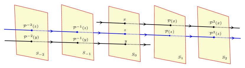
Remark 6.7.

In geometric meaning, Proposition 6.6 says that, if the future orbit $\{\varphi_{t}(x),t\geq 0\}$ of $x\in{\rm int\,}S_{0}$ passes through ${\rm int\,}S_{1},i=1,2,3,\dots$ (in sequence) and the past orbit $\{\varphi_{t}(y),t<0\}$ of $y\in{\rm int\,}S_{0}$ passes through ${\rm int\,}S_{i},i=-1,-2,\dots$ (in sequence) then the orbit of $\langle x,y\rangle_{S_{0}}\in{\rm int\,}S_{0}$ has both properties; see Figure 6 for an illustration. This property is used as the definition of Markov partitions in [15]. $\Diamond$

Figure 6: Markov property: $z=\langle x,y\rangle_{T_{x_{0}}}$ has properties of both $x$ and $y$

In the rest of this paper we prove the following main result.

Theorem 6.8.

The flow $(\varphi_{t})_{t\in\mathbb{R}}$ has a Markov partition of arbitrary small size.

The construction of Markov partitions can be summarized as follows.

• For arbitrarily small $\alpha>0$, construct a proper family of size $\alpha$ consisting of rectangles $B_{1},\dots,B_{n}$ rectangles, which contain rectangles $K_{1},\dots,K_{n}$ with certain properties (Theorem 6.9).

• Enlarge rectangles $K_{1},\dots,K_{n}$ to $C_{1},\dots,C_{n}$ satisfying Lemma 6.12.

• Decompose $C_{i}$ into smaller sets $E_{ji}^{1},E_{ji}^{2},E_{ji}^{3},E_{ji}^{4}$ in Lemma 6.16 and define family ${\mathfrak{C}}_{i}$ of sets in $C_{i}$; see Lemma 6.17.

• Construct equivalence classes of elements in $C_{i}$ whose orbits visit the same member of ${\mathfrak{C}}_{1},\dots\mathfrak{C}_{n}$ in the same order for sufficiently large times.

• Prove that after sliding appropriately small times, these equivalence classes are a Markov partition; see lemmas 6.18 and 6.19.

Fix $\varepsilon\in(0,\sigma_{*}/5)$ and define $\delta_{1}=\delta(\varepsilon)$ from Corollary 3.3, and $\delta_{2}=\delta(\varepsilon)$ as in Lemma 5.3. We define $\delta=\min\{\delta_{1}/4,\delta_{2}/4,\sigma_{*}/6\}$ and consider $\alpha\in(0,\delta)$.

First, we construct a so-called pre-Markov partition, which is stated in [6] without a proof. A similar assertion can be found in [14].

Theorem 6.9.

There are a family of differentiable local cross sections ${\mathscr{D}}=\{D_{1},\dots,D_{n}\}$ and two families of rectangles $\mathscr{K}=\{K_{1},\dots,K_{n}\},\mathscr{B}=\{B_{1},\dots,B_{n}\}$ satisfying

1. $K_{i}\subset{\rm int\,}B_{i},B_{i}\subset{\rm int\,}D_{i},i=1,\dots,n$;

2. ${\rm diam\,}D_{i}<\alpha,i=1,\dots,n$;

3. for $i\neq j$, at least one of the sets $D_{i}\bigcap\varphi_{[0,2\alpha]}(D_{j})$ and $D_{j}\bigcap\varphi_{[0,2\alpha]}(D_{i})$ is empty;

4. $X=\varphi_{[-\alpha,0]}(\bigcup_{i=1}^{n}{\rm int\,}K_{i})=\varphi_{[-\alpha,0]}(\bigcup_{i=1}^{n}{\rm int\,}B_{i})$;

5. if $B_{i}\bigcap\varphi_{[-\alpha,\alpha]}(B_{j})\neq\varnothing$, then $B_{i}\subset\varphi_{[-2\alpha,2\alpha]}(D_{j})$.

In comparison with the statement in [6], there is a slightly difference of the flow times and the presence of $K_{1},\dots,K_{n}$. Later in our construction, we will enlarge $K_{1},\dots,K_{n}$ to $C_{1},\dots,C_{n}$, which are still included in $B_{1},\dots,B_{n}$, and conditions (c), (e) will be crucial in proving the Markov property.

Proof.

The idea of this proof is carefully modified from that of [7, Lemma 7].

Note that due to $0<\alpha<\sigma_{*}/6$, any Poincaré section of radius at most $\lambda$ is a local cross section of time $2\alpha$; see Lemma 4.2. Since $X$ is compact, there are $x_{1},\dots,x_{m}\in X$ pairwise disjoint such that

$$X=\varphi_{[-\alpha,0]}({\rm int\,}S_{\alpha/16}(x_{1}))\cup\bigcup_{k=2}^{m}\varphi_{[-\alpha,0]}({\rm int\,}P_{\alpha/2}({x_{k}})).$$ (6.30)

Step 1: First, we construct ${\cal D}$ and ${\cal K}$ recursively. Set ${\cal D}_{1}=\{P_{\alpha/4}(x_{1})\}$ and ${\cal K}_{1}=\{S_{\alpha/16}(x_{1})\}$. For each $y\in P_{\alpha/2}(x_{2})$, the set $\varphi_{[-2\alpha,2\alpha]}(y)\cap P_{\alpha/2}(x_{1})$ is either one single point or empty, due to the fact that $P_{\alpha/2}(x_{1})$ is a local cross section of time at least $2\alpha$. This yields that there is $t_{y}\in(-2\alpha,2\alpha)$ such that $\varphi_{t_{y}}(y)\notin P_{\alpha}(x_{1})$. Since $X\setminus P_{\alpha/2}(x_{1})$ is an open, using the continuity of the flow $\varphi:\mathbb{R}\times X\to X$, there are an open interval $I_{y}\subset(-2\alpha,2\alpha)$ and an open neighbourhood $V_{y}\subset P_{\alpha}(x_{2})$ of $y$ so that $\varphi_{I_{y}}(V_{y})\subset X\setminus P_{\alpha/2}(x_{1})$, or equivalently, $\varphi_{I_{y}}(V_{y})\cap P_{\alpha/2}(x_{1})=\varnothing$. Take $0<r_{y}<\alpha/4$ so small that $P_{r_{y}}(y)\subset V_{y}$ to have

$$\varphi_{I_{y}}(P_{r_{y}}(y))\cap P_{\alpha/2}(x_{1})=\varnothing.$$

Due to the fact that $P_{\alpha/2}(x_{2})$ is compact, there are $y_{1},\dots,y_{n_{2}}\in P_{\alpha/2}(x_{2})$ distinct such that $P_{r_{y_{i}}}(y_{i})\subset P_{\alpha}(x_{2})$ and

$$P_{\alpha/2}(x_{2})\subset\bigcup_{i=1}^{n_{2}}{\rm int\,}S_{r_{y_{i}}/8}(y_{i}).$$

Pick distinct numbers $u_{1}\in I_{y_{1}},\dots,u_{n_{2}}\in I_{y_{n_{2}}}$ and set

$${\cal D}_{2} ={\cal D}_{1}\cup\{\varphi_{u_{1}}(P_{r_{y_{1}}}(y_{1})),\dots,\varphi_{u_{n_{2}}}(P_{r_{y_{n_{2}}}}(y_{n_{2}}))\},$$

$${\cal K}_{2} ={\cal K}_{1}\cup\{\varphi_{u_{1}}(S_{{r_{y_{1}}}/8}(y_{1})),\dots,\varphi_{u_{n_{2}}}(S_{r_{y_{n_{2}}}/8}(y_{n_{2}}))\}.$$

Owing to that $u_{1},\dots,u_{n_{2}}$ are distinct, we see that Poincaré sections in ${\cal D}_{2}$ are pairwise disjoint satisfy Condition (c). Suppose that ${\cal D}_{3},\dots,{\cal D}_{k-1}$, ${\cal K}_{3},\dots,{\cal K}_{k-1}$ are similarly constructed for $k\leq m$ and all Poincaré sections in ${\cal D}_{k-1}$ satisfy Condition (c). We are going to construct ${\cal D}_{k}$ and ${\cal K}_{k}$. Analogously to the construction of ${\cal D}_{2}$, for every $z\in P_{\alpha/2}(x_{k})$, the set

$$\varphi_{[-2\alpha,2\alpha]}(z)\cap{\tt D}_{k-1}$$

is a set of finite points since ${\cal D}_{k-1}$ consists of finitely many local cross sections of times at least $2\alpha$; here ${\tt D}_{k-1}$ denotes the union of elements in ${\cal D}_{k-1}$. Using the continuity of the flow, there exist an open interval $I_{z}\subset(-2\alpha,2\alpha)$ and $0<r_{z}<\alpha/4$ such that $\varphi_{I_{z}}(P_{r_{z}}(z))\cap{\tt D}_{k-1}=\varnothing$. We cover $P_{\alpha/2}(x_{k})$ by smaller rectangles $S_{r_{z_{i}}/8}(z_{i})\subset P_{r_{z_{i}}}(z_{i})\subset P_{\alpha}(x_{k})$:

$$P_{\alpha/2}(x_{k})\subset\bigcup_{i=1}^{n_{k}}{\rm int\,}S_{r_{z_{i}}/8}(z_{i}),$$ (6.31)

where $z_{i}\in P_{\alpha/2}(x_{k})$. Pick distinct numbers $u_{1}\in I_{z_{1}},\dots,u_{n_{k}}\in I_{z_{n_{k}}}$ and let

$${\cal D}_{k} ={\cal D}_{k-1}\cup\{\varphi_{v_{1}}(P_{r_{z_{1}}}(z_{1})),\dots,\varphi_{v_{n_{k}}}(P_{r_{z_{n_{k}}}}(z_{n_{k}}))\},$$

$${\cal K}_{k} ={\cal K}_{k-1}\cup\{\varphi_{v_{1}}(S_{r_{z_{1}}/8}(z_{1})),\dots,\varphi_{v_{n_{k}}}(S_{r_{z_{n_{k}}}/8}(z_{n_{k}}))\}.$$

Due to the radii of elements in ${\cal D}_{k}$ is at most $\alpha/4$, their radii are at most $\alpha$ and hence ${\cal D}_{k}$ satisfies Condition (b). Next we check that the elements in ${\cal D}_{k}$ satisfy Condition (c). Suppose that $\varphi_{[-2\alpha,2\alpha]}(P_{i})\cap P\neq\varnothing$ with $P\in{\cal D}_{k-1}$ and $P_{i}=\varphi_{v_{i}}(P_{r_{z_{i}}}(z_{i}))$ for some $i$. If $v_{i}\geq 0$, then $\varphi_{[0,2\alpha]}(P)\cap P_{i}=\varnothing$ and if $v_{i}<0$ then $\varphi_{[0,2\alpha]}(P_{i})\cap P=\varnothing$. Let $P_{i}=\varphi_{v_{i}}(P_{r_{z_{i}}}(z_{i})),P_{j}=\varphi_{v_{j}}(P_{r_{z_{j}}}(z_{j})),i\neq j$. If $v_{i}>v_{j}$ then we observe that $\varphi_{[0,2\alpha]}(P_{i})\cap P_{j}=\varnothing$. For, suppose on the contrary that there is $w=\varphi_{t}(u)\in P_{j}$ for $t\in[0,2\alpha]$ and $u\in P_{i}$. Then $w=\varphi_{v_{j}}(w^{\prime})$ and $u=\varphi_{v_{i}}(u^{\prime})$ for $u^{\prime}\in P_{r_{z_{i}}}(z_{i})\subset P_{\alpha}(x_{k}),w^{\prime}\in P_{r_{z_{j}}}(z_{j})\subset P_{\alpha}(x_{k})$ imply that $w=\varphi_{t+v_{i}}(u^{\prime})=\varphi_{v_{j}}(w^{\prime})$. Since $P_{\alpha}(x_{k})$ is a local cross section, we have $u^{\prime}=w^{\prime}$ and hence $t+v_{i}=v_{j}$ or $t=v_{j}-v_{i}<0$, contradicting $t\geq 0$. Similarly, if $v_{i}<v_{j}$, then $P_{i}\cap\varphi_{[0,2\alpha]}(P_{j})=\varnothing$. We have shown that if $P,Q\in{\cal D}_{k}$ and $P\neq Q$, then at least one of the sets $\varphi_{[0,2\alpha]}(P)\cap Q$ and $\varphi_{[0,2\alpha]}(Q)\cap P$ is empty. Therefore, ${\cal D}_{k}$ satisfies Condition (c).

Repeating this process, we obtain

$${\cal D}_{m} = {\cal D}_{m-1}\cup\{\varphi_{p_{1}}(P_{r_{w_{1}}}(w_{1})),\dots,\varphi_{p_{n_{m}}}(P_{r_{w_{n_{m}}}}(w_{n_{m}}))\},$$

$${\cal K}_{m} = {\cal K}_{m-1}\cup\{\varphi_{p_{1}}(S_{r_{w_{1}}/8}(w_{1})),\dots,\varphi_{p_{n_{m}}}(S_{r_{w_{n_{m}}}/8}(w_{n_{m}}))\},$$

where $p_{1}\in I_{w_{1}},\dots,p_{n_{m}}\in I_{w_{n_{m}}}$ are pairwise distinct, $I_{w_{1}},\dots,I_{w_{n_{m}}}\subset(-2\alpha,2\alpha)$ and $0<r_{w_{i}}<\alpha/4$ such that

$$P_{\alpha/2}(x_{m})\subset\bigcup_{i=1}^{n_{m}}{\rm int\,}S_{r_{w_{i}}/8}(w_{i})\quad\mbox{and}\quad\varphi_{I_{w_{j}}}(P_{r_{w_{j}}}(w_{j}))\cap{\tt D}_{m-1}=\varnothing,$$

where ${\tt D}_{m-1}$ denotes the union of sets in ${\cal D}_{m-1}$, $S_{r_{w_{i}}/8}(w_{i})\subset P_{r_{w_{i}}}(w_{i})\subset P_{\alpha}(x_{k})$.

Let $n={\rm card\,}{\cal D}_{m}$ and denote the elements in ${\cal D}_{m}$ and ${\cal K}_{m}$ by $D_{1},\dots,D_{n}$, and $K_{1},\dots,K_{n}$, respectively. In summary, we have constructed a family of cross sections $D_{1}\dots,D_{n}$ satisfying conditions (b) and (c). In addition, due to $\varphi_{t}(\Gamma gc_{u}b_{s})=\Gamma ga_{t}c_{ue^{t}}b_{se^{-t}}$ for $g\in{\rm PSL}(2,\mathbb{R}),t,u,s\in\mathbb{R}$, by correcting the radii of Poincaré sections $D_{i}$ and rectangles $K_{i}$, we may assume that

$$D_{i}=P_{4\varepsilon}(z_{i})\quad\mbox{and}\quad K_{i}=S_{\varepsilon/2}(z_{i})$$

for $z_{i}\in X$ and some $\varepsilon\in(0,\alpha/16)$. Then $D_{i}=P_{4\varepsilon}(z_{i})\subset P_{\alpha/4}(z_{i})$, so (b) holds by Lemma 4.2. Now, for each $i\in\{1,\dots,n\}$, define

$$B_{i}=S_{\varepsilon}(z_{i}).$$

to obtain (a).

Step 2: Proof of (d). Due to (6.30), for any $x\in X$, either $x\in\varphi_{[-\alpha,0]}(S_{\alpha/16}(x_{1}))$ or $x\in\varphi_{[-\alpha,0]}({\rm int\,}P_{\alpha/2}(x_{k}))$ for some $k\in\{2,\dots,m\}$. Then (6.31) implies that $x\in\varphi_{[-\alpha,0]}({\rm int\,}S_{r_{z_{i}}/8}(z_{i}))$ for some $i\in\{1,\dots,r_{n_{k}}\}$. This means that $x\in\varphi_{[-\alpha,0]}({\rm int\,}K_{s})$ for some $s\in\{1,\dots,n\}$, and the former of (d) is proved. This yields the latter of (d).

Step 3: Proof of (e). Write $z_{i}=\Gamma g_{i}$ for $g_{i}\in{\rm PSL}(2,\mathbb{R})$. Suppose that $x=\varphi_{t}(y)$ for $t\in[-\alpha,\alpha]$, $x\in B_{i}$ and $y\in B_{j}$. We need to check that $x\in\varphi_{[-2\alpha,2\alpha]}(D_{j})$. Recall that for $k\in\{1,\dots,n\}$,

$$B_{k}=S_{\varepsilon}({z_{k}})=\{\Gamma g_{k}c_{u}b_{s},u\in[-\varepsilon,\varepsilon],s=\frac{s^{\prime}}{1-us^{\prime}}\ \mbox{for some}\ s^{\prime}\in[-\varepsilon,\varepsilon]\}.$$

We have $x=\Gamma g_{i}c_{u}b_{s}=\Gamma g_{j}c_{\hat{u}}b_{\hat{s}}a_{t}$. For any $z=\Gamma g_{i}c_{\tilde{u}}b_{\tilde{s}}\in B_{i}$, we write

$$z \ =\Gamma g_{i}c_{u}b_{s}b_{-s}c_{-u}c_{\tilde{u}}b_{\tilde{s}}=\Gamma g_{j}c_{\hat{u}}b_{\hat{s}}a_{t}b_{-s}c_{-u}c_{\tilde{u}}b_{\tilde{s}}$$

$$\ =\Gamma g_{j}c_{\hat{u}}b_{\hat{s}-se^{t}}c_{(\tilde{u}-u)e^{-t}}b_{\tilde{s}e^{t}}a_{t}=\Gamma g_{j}c_{\bar{u}}b_{\bar{s}}a_{\bar{t}},$$

where

$$\bar{s} \ =\hat{s}-se^{t}+\tilde{s}e^{t}+(\tilde{u}-u)e^{-t}(\hat{s}-se^{t})(1+\hat{s}-se^{t}+\tilde{s}e^{t})$$

$$\ \ \ \ \ +(\tilde{u}-u)(\hat{s}-se^{t})\tilde{s}(1+(\tilde{u}-u)e^{-t}(\hat{s}-se^{t})),$$

$$\bar{u} \ =\hat{u}+(\tilde{u}-u)e^{-t}-\frac{(\tilde{u}-u)^{2}e^{-2t}({\hat{s}-se^{t}})}{1+(\tilde{u}-u)e^{-t}({\hat{s}-se^{t}})},$$

$$\bar{t} \ =t+2\ln(1+(\tilde{u}-u)e^{-t}({\hat{s}-se^{t}})).$$

After a short calculation, we obtain $|\bar{t}|\leq 2\alpha,|\bar{s}|<4\varepsilon,|\bar{u}|<4\varepsilon$. This means that $z\in\varphi_{[-2\alpha,2\alpha]}(D_{j})$, proving Condition (e).

The theorem is proved. ∎

From the above proof, it follows the next result.

Remark 6.10.

With the setting in Theorem 6.9,

(e’) if $B_{i}\bigcap\varphi_{[-\alpha,0]}(B_{j})\neq\varnothing$ then $B_{i}\subset\varphi_{[-2\alpha,0]}(D_{j})$ and if $B_{i}\bigcap\varphi_{[0,\alpha]}(B_{j})\neq\varnothing$ then $B_{i}\subset\varphi_{[0,2\alpha]}(D_{j})$. $\Diamond$

Now, recall that $X=\varphi_{[-\alpha,0]}(\bigcup_{i=1}^{n}K_{i})=\varphi_{[-\alpha/2,\alpha/2]}(\bigcup_{i=1}^{n}K_{i})$. Let $3\lambda>0$ be the Lebesgue number for the cover $\{\varphi_{[-\alpha/2,\alpha/2]}(K_{1}),\dots,\varphi_{[-\alpha/2,\alpha/2]}(K_{n})\}$, i.e., any subset of $X$ with diameter at most $3\lambda$ contains in some $\varphi_{[-\alpha/2,\alpha/2]}(K_{i})$. Fix $L>0$ and $i\in\{1,\dots,n\}$. For $x\in K_{i}$, there is a closed neighbourhood $V_{x}^{i}$ of $x$ such that

$${\rm diam\,}\varphi_{t}(V_{x}^{i})\leq\lambda\quad\mbox{for all}\quad|t|\leq 2L.$$

Since $K_{i}$ compact, we cover it by a finite family ${\cal V}_{i}=\{V^{i}_{x_{1}},\dots,V^{i}_{x_{n_{i}}}\}$:

$$K_{i}\subset\bigcup_{j=1}^{n_{i}}V^{i}_{x_{j}}.$$

We may assume that for any $V\in{\cal V}_{i}$, $V\subset S_{2\varepsilon/3}(z_{i})$.

Let $A\subset X$ be given. Denote

$$B(A,\lambda)=\{x\in X:d_{X}(x,A)=\inf_{y\in A}d_{X}(x,y)<\lambda\}.$$

We claim that ${\rm diam\,}B(\varphi_{-L}(V),\lambda)<3\lambda$ and ${\rm diam\,}B(\varphi_{L}(V),\lambda)<3\lambda$ for all $V\in{\cal V}_{i}$. For, taking $x,y\in B(\varphi_{-L}(V),\lambda)$, there are $z_{1},z_{2}\in\varphi_{-L}(V)$ such that $d_{X}(x,z_{1})<\lambda$ and $d_{X}(y,z_{2})<\lambda$. This implies $d_{X}(x,y)\leq d_{X}(x,z_{1})+d_{X}(z_{1},z_{2})+d_{X}(z_{2},y)<3\lambda$ and hence ${\rm diam\,}B(\varphi_{-L}(V),\lambda)<3\lambda$. Similarly, ${\rm diam\,}B(\varphi_{L}(V),\lambda)<3\lambda$.

By the property of $\lambda$, for each $i\in\{1,\dots,n\}$ and $V\in{\cal V}_{i}$, there are $a(V),b(V)\in\{1,\dots,n\}$ so that $B(\varphi_{-L}(V),\lambda)\subset\varphi_{[-\alpha/2,\alpha/2]}(K_{a(V)})$ and $B(\varphi_{L}(V),\lambda)\subset\varphi_{[-\alpha/2,\alpha/2]}(K_{b(V)})$. Then the following maps

$$g_{V^{-}}={\rm pr}_{D_{a(V)}}\circ\varphi_{-L}:V\longrightarrow K_{a(V)}\subset B_{a(V)}$$

and

$$g_{V^{+}}={\rm pr}_{D_{b(V)}}\circ\varphi_{L}:V\longrightarrow K_{b(V)}\subset B_{b(V)}$$

are well-defined. We recursively define the set $R_{i,k}$ and $S_{i,k}$ by $R_{i,0}=S_{i,0}=K_{i}$ and for $k\geq 0$

$$R_{i,k+1} =\bigcup\limits_{V\in{\cal V}_{i}}\bigcup\limits_{v\in V}\{\langle y,{\rm pr}_{D_{i}}\varphi_{L}(z)\rangle_{D_{i}}:y\in K_{i},z\in W^{s}(g_{V^{-}}(v),R_{a(V),k})\},$$ (6.32)

$$S_{i,k+1} =\bigcup\limits_{V\in{\cal V}_{i}}\bigcup\limits_{v\in V}\{\langle{\rm pr}_{D_{i}}\varphi_{-L}(z),y\rangle_{D_{i}}:y\in K_{i},z\in W^{u}(g_{V^{+}}(v),S_{b(V),k})\}.$$ (6.33)

For $x\in(0,1)$, we set $x^{\prime}=\frac{x}{1-x^{2}}$. Note that $x<y$ if and only if $x^{\prime}<y^{\prime}$ and $x=y$ if and only if $x^{\prime}=y^{\prime}$.

In the rest of the paper, we consider $L>4$ and $T:=L-\alpha/2$. Define $\varepsilon_{0}=2\varepsilon/3$ and $\varepsilon_{k+1}=\varepsilon_{0}+2\varepsilon_{k}e^{-T},k\geq 0$. Accordingly, $\varepsilon_{0}^{\prime}=2\varepsilon^{\prime}/3$ and $\varepsilon_{k+1}^{\prime}=\varepsilon_{0}^{\prime}+2\varepsilon_{k}^{\prime}e^{-T}$, $k\geq 0$.

Lemma 6.11.

For every $i\in\{1,\dots,n\}$, the following statements hold.

(a) $R_{i,k}\subset S_{\varepsilon_{0}}^{\varepsilon_{k}}(z_{i})$ and $S_{i,k}\subset S^{\varepsilon_{k}}_{\varepsilon_{0}}(z_{i})$ for all $k\geq 0$.

(b) The sets $R_{i}=\bigcup\limits_{k=0}^{\infty}R_{i,k},\,S_{i}=\bigcup\limits_{k=0}^{\infty}S_{i,k}$ are subsets of $B_{i}$.

(c) The set $C_{i}=\langle S_{i},R_{i}\rangle_{D_{i}}=\{\langle p,q\rangle_{D_{i}}:p\in S_{i},q\in R_{i}\}$ is a rectangle contained in $B_{i}$.

Proof.

(a) We prove the former by induction. First,

$$R_{i,1}=\underset{V\in{\cal V}_{i}}{\bigcup}\bigcup_{v\in V}\{\langle y,{\rm pr}_{D_{i}}\varphi_{L}(z)\rangle_{D_{i}}:y\in K_{i},z\in W^{s}(g_{V^{-}}(v),K_{a(V)})\}.$$

For any $x\in R_{i,1}$, $x=\langle y,{\rm pr}_{D_{i}}\varphi_{L}(z)\rangle_{D_{i}}$ for $z\in W^{s}({\rm pr}_{D_{a(V)}}\varphi_{-L}(v),K_{a(V)})$ with some $v\in V\in{\cal V}_{i}$. We first show that ${\rm pr}_{D_{i}}\varphi_{L}(z)\in S_{\varepsilon_{0}}^{\varepsilon_{1}}(z_{i})$. Let $v=\Gamma g_{i}c_{u_{v}}b_{s_{v}}\in V\subset S_{2\varepsilon/3}(z_{i})$ and ${\rm pr}_{D_{a(V)}}\varphi_{-L}(v)=\varphi_{-L-\tau}(v)=\Gamma g_{l}c_{u}b_{s}\in K_{l}=S_{\varepsilon/2}(\Gamma g_{l})$ with $l={a(V)}\in\{1,\dots,n\}$ for some $\tau\in[-\alpha/2,\alpha/2]$. According to Proposition 4.14 (a), $z=\Gamma g_{l}c_{u}b_{s_{z}}$. Since $\varphi_{L+\tau}({\rm pr}_{D_{a(V)}}\varphi_{-L}(v))=v$, it follows that $\Gamma g_{l}c_{u}b_{s}a_{L+\tau}=\Gamma g_{i}c_{u_{v}}b_{s_{v}}$. This implies that

$$\hat{z}:=\varphi_{L+\tau}(z)=\Gamma g_{l}c_{u}b_{s}a_{L+\tau}b_{(s_{z}-s)e^{-L-\tau}}=\Gamma g_{i}c_{u_{v}}b_{s_{v}+(s_{z}-s)e^{-L-\tau}}\in D_{i}.$$

Also $\hat{z}={\rm pr}_{D_{i}}\varphi_{L}(z)=(u_{\hat{z}},s_{\hat{z}})_{z_{i}}\in D_{i}$, where

$$u_{\hat{z}}=u_{v}\ \mbox{ and }\ s_{\hat{z}}=(u,s_{v}+(s_{z}-s)e^{-L-\tau})_{z_{i}}.$$

Then

$$|s_{\hat{z}}|\leq\varepsilon_{0}^{\prime}+2\varepsilon_{0}^{\prime}e^{-L+\alpha/2}\leq\varepsilon_{0}^{\prime}+2\varepsilon_{0}^{\prime}e^{-T}=\varepsilon_{1}^{\prime}$$

shows that $\hat{z}\in S^{\varepsilon_{1}}_{\varepsilon_{0}}(z_{i})$. Since $y\in K_{i}=S_{\varepsilon}(z_{i})\subset S_{\varepsilon_{0}}^{\varepsilon_{1}}(z_{i})$, we get $x=\langle y,\hat{z}\rangle_{D_{i}}\in S_{\varepsilon_{0}}^{\varepsilon_{1}}(z_{i})$ due to the fact that $S_{\varepsilon_{0}}^{\varepsilon_{1}}(z_{i})$ is a rectangle. Therefore $R_{i,1}\subset S_{\varepsilon_{0}}^{\varepsilon_{1}}(z_{i})$.

Next, assume that $R_{i,j-1}\in S^{\varepsilon_{j-1}}_{\varepsilon_{0}}(z_{i})$ for $j>1$. Take $x=\langle y,{\rm pr}_{D_{i}}\varphi_{L}(z)\rangle_{D_{i}}\in R_{i,j}$, where $y\in K_{i}$, $z\in W^{s}({\rm pr}_{D_{a(V)}}\varphi_{-L}(v),R_{a(V),j-1})$ for some $v=\Gamma g_{i}c_{u_{v}}b_{s_{v}}\in V\in{\cal V}_{i}$. Similarly to above, ${\rm pr}_{D_{a(V)}}\varphi_{-L}(v)=\varphi_{-L-\tau}(v)=\Gamma g_{l}c_{u}b_{s}\in R_{l,j-1}$ with $l={a(V)}$ for some $\tau\in[-\alpha/2,\alpha/2]$. Writing $z=\Gamma g_{l}c_{u}b_{s_{z}}$, we have

$$\hat{z}:= \ {\rm pr}_{D_{i}}\varphi_{-L}(z)=\varphi_{L+\tau}(z)=\Gamma g_{l}c_{u}b_{s}a_{L+\tau}b_{(s_{z}-s)e^{-L-\tau}}$$

$$= \ \Gamma g_{i}c_{u_{v}}b_{s_{v}+(s_{z}-s)e^{-L-\tau}}=(u_{\hat{z}},s_{\hat{z}})_{z_{i}}\in D_{i},$$

where

$$u_{\hat{z}}=u_{v},\ s_{\hat{z}}=s_{v}+(s_{z}-s)e^{-L-\tau}.$$

Then

$$|s_{\hat{z}}|\leq\varepsilon^{\prime}_{0}+2\varepsilon^{\prime}_{j-1}e^{-T}=\varepsilon^{\prime}_{j}$$

yields $\hat{z}\in S^{\varepsilon_{j}}_{\varepsilon_{0}}(z_{i})$. Since $y\in K_{i}\subset S_{\varepsilon_{0}}^{\varepsilon_{j}}(z_{i})$, we obtain $x=\langle y,\hat{z}\rangle_{D_{i}}\in S_{\varepsilon_{0}}^{\varepsilon_{j}}(z_{i})$ and so $R_{i,j}\subset S_{\varepsilon_{0}}^{\varepsilon_{j}}(z_{i})$. We deduce that $R_{i,k}\subset S_{\varepsilon_{0}}^{\varepsilon_{k}}(z_{i})$ for all $k\geq 0$.

To verify the latter, we need the other versions of Poincaré sections and rectangles. Define

$$\widetilde{D}_{i}=\widetilde{P}_{4\varepsilon}(z_{i})=\{\Gamma g_{i}b_{s}c_{u}:u,s\in[-4\varepsilon,4\varepsilon]\}$$

and

$$\widetilde{B}_{i}=T_{\varepsilon}(z_{i})=\{\Gamma g_{i}b_{s}c_{u}:s\in[-\varepsilon,\varepsilon]\mbox{ and }u=\frac{u^{\prime}}{1-su^{\prime}}\quad\mbox{ for some }u^{\prime}\in[-\varepsilon,\varepsilon]\}.$$

We recall from Lemma 4.13 that ${\rm pr}_{D_{i}}(\widetilde{B}_{i})=B_{i}$ and ${\rm pr}_{\widetilde{D}_{i}}(B_{i})=\widetilde{B}_{i}$. By projecting to $\widetilde{D}_{i}$, (6.33) is equivalent to

$$\widetilde{S}_{i,k+1}=\bigcup\limits_{\widetilde{V}\in\widetilde{\cal V}_{i}}\bigcup\limits_{v\in\widetilde{V}}\{\langle{\rm pr}_{\widetilde{D}_{i}}\varphi_{-L}(z),y\rangle_{\widetilde{D}_{i}}:y\in\widetilde{K}_{i},z\in W^{u}(g_{\widetilde{V}^{+}}(v),S_{b(\widetilde{V}),k})\},$$ (6.34)

where $\widetilde{S}_{i,k}={\rm pr}_{\widetilde{D}_{i}}(S_{i,k}),$ $\widetilde{K}_{i}={\rm pr}_{\widetilde{D}_{i}}(K_{i})$, $\widetilde{\cal V}_{i}={\rm pr}_{\widetilde{D}_{i}}({\cal V}_{i})$, $\widetilde{V}_{i}={\rm pr}_{\widetilde{D}_{i}}(V_{i})$, and

$$g_{\widetilde{V}^{+}}={\rm pr}_{\widetilde{D}_{b(\widetilde{V})}}\circ\varphi_{L}:\widetilde{V}\longrightarrow\widetilde{K}_{b(\widetilde{V})}\subset\widetilde{B}_{b(\widetilde{V})}.$$

Recall from Proposition 4.13 that ${\rm pr}_{\widetilde{D}_{i}}(S_{\varepsilon_{0}}^{\varepsilon_{k}}(z_{i}))=T^{\varepsilon_{0}}_{\varepsilon_{k}}(z_{i})$ and ${\rm pr}_{D_{i}}(T^{\varepsilon_{0}}_{\varepsilon_{k}}(z_{i}))=S_{\varepsilon_{0}}^{\varepsilon_{k}}(z_{i})$. Together with ${\rm pr}_{D_{i}}(\widetilde{S}_{i,k})=S_{i,k}$, the inclusion $S_{i,k}\subset S_{\varepsilon_{k}}^{\varepsilon_{0}}(z_{i})$ is equivalent to

$$\widetilde{S}_{i,k}\subset T_{\varepsilon_{0}}^{\varepsilon_{k}}(z_{i}).$$ (6.35)

We first verify that $\widetilde{S}_{i,1}\subset T_{\varepsilon_{0}}^{\varepsilon_{1}}(z_{i})$. For $x\in\widetilde{S}_{i,1}$, $x=\langle{\rm pr}_{\widetilde{D}_{i}}\varphi_{-L}(z),y\rangle_{\widetilde{D}_{i}}$, where $y\in\widetilde{K}_{i}$ and $z\in W^{u}({\rm pr}_{\widetilde{D}_{b(\widetilde{V})}}\varphi_{L}(v),\widetilde{K}_{b(\widetilde{V})})$ for $v=\Gamma g_{i}b_{s_{v}}c_{u_{v}}\in\widetilde{V}\in\widetilde{\cal V}_{i}$. There is a $\tau\in[-\alpha/2,\alpha/2]$ such that ${\rm pr}_{\widetilde{D}_{b(\widetilde{V})}}\varphi_{L}(v)=\varphi_{L+\tau}(v)=\Gamma g_{l}b_{s}c_{u}\in\tilde{K}_{l}=T_{\varepsilon/2}(\Gamma g_{l})$ for $l={b(\widetilde{V})}$. By Proposition 4.14 (b), $z=\Gamma g_{l}b_{s}c_{u_{z}}$. Since $\varphi_{-L-\tau}({\rm pr}_{\widetilde{D}_{b(\widetilde{V})}}\varphi_{L}(v))=v$, it follows that $\Gamma g_{l}b_{s}c_{u}a_{-L-\tau}=\Gamma g_{i}b_{s_{v}}c_{u_{v}}$. Then

$$\hat{z}:=\varphi_{-L-\tau}(z)=\Gamma g_{l}b_{s}c_{u}a_{L+\tau}c_{(u_{z}-u)e^{-L-\tau}}=\Gamma g_{i}b_{s}c_{u_{v}+(u_{z}-u)e^{-L-\tau}}\in\widetilde{D}_{i}$$

implies that

$$\hat{z}={\rm pr}_{\widetilde{D}_{i}}\varphi_{-L}(z)=(s_{\hat{z}},u_{\hat{z}})_{z_{i}}^{\prime},$$

where

$$s_{\hat{z}}=s,\ u_{\hat{z}}=u_{v}+(u_{z}-u)e^{-L-\tau}.$$

The estimate

$$|u_{\hat{z}}|\leq\varepsilon_{0}^{\prime}+2\varepsilon_{0}^{\prime}e^{-L+\alpha/2}\leq\varepsilon_{0}^{\prime}+2\varepsilon_{0}^{\prime}e^{-T}=\varepsilon_{1}^{\prime}$$

shows that $\hat{z}\in T^{\varepsilon_{0}}_{\varepsilon_{1}}(z_{i})$. Since $y\in\tilde{K}_{i}=T_{\varepsilon/2}(z_{i})\subset T_{\varepsilon_{1}}^{\varepsilon_{0}}(z_{i})$, we have $x\in T^{\varepsilon_{0}}_{\varepsilon_{1}}(z_{i})$ due to the fact that $T^{\varepsilon_{0}}_{\varepsilon_{1}}(z_{i})$ is a rectangle, and we deduce $\widetilde{S}_{i,1}\subset T^{\varepsilon_{0}}_{\varepsilon_{1}}(z_{i})$. In the similar way, we can show that if $\widetilde{S}_{i,j-1}\subset T^{\varepsilon_{0}}_{\varepsilon_{j-1}}(z_{i})$ for $i>1$, then $\widetilde{S}_{i,j}(z_{i})\subset T^{\varepsilon_{0}}_{\varepsilon_{j}}(z_{i})$ and hence (6.34) is obtained.

(b) We have

$$\varepsilon_{k} =\varepsilon_{0}+\varepsilon_{0}(2e^{-T})+\dots+\varepsilon_{0}(2e^{-T})^{k-1}+\varepsilon_{0}(2e^{-T})^{k}$$

$$=\frac{1-(2e^{-T})^{k+1}}{1-2e^{-T}}\varepsilon_{0}<\frac{\varepsilon_{0}}{1-2e^{-T}}<\frac{3}{2}\varepsilon_{0}=\varepsilon.$$

for all $k\geq 1$ when $T>3$. This implies that $S_{\varepsilon_{0}}^{\varepsilon_{k}}(z_{i})\subset S_{\varepsilon}(z_{i})=B_{i}$ and $S^{\varepsilon_{0}}_{\varepsilon_{k}}(z_{i})\subset S_{\varepsilon}(z_{i})=B_{i}$ for all $k\geq 1$. Therefore $R_{i}=\bigcup\limits_{k=0}^{\infty}R_{i,k}\subset B_{i}$ and $S_{i}=\bigcup\limits_{k=0}^{\infty}S_{i,k}\subset B_{i}$.

(c) If $x_{i}=\langle p_{i},q_{i}\rangle_{D_{i}}\in C_{i},i=1,2$, then $\langle x_{1},x_{2}\rangle_{D_{i}}=\langle\langle p_{1},q_{1}\rangle_{D_{i}},\langle p_{2},q_{2}\rangle_{D_{i}}\rangle_{D_{i}}=\langle p_{1},q_{2}\rangle_{D_{i}}\in C_{i}$ by Lemma 4.18 (d). This shows that each $C_{i}$ is a rectangle. Due to (b), it follows that $C_{i}\subset B_{i}$. ∎

Figure 7: Illustration for the proof of Lemma 6.12

The next lemma is a key result, which help us prove the final statement (Lemma 6.19).

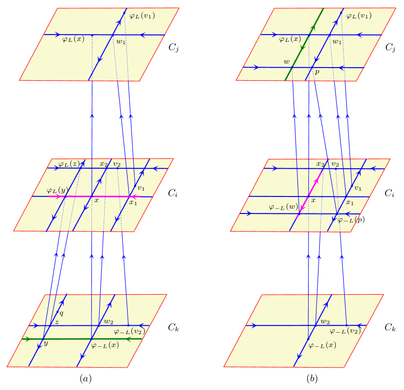
Lemma 6.12.

Consider $x\in C_{i}$.

(a) There is a $k$ so that

$$\varphi_{-L}(x)\in\varphi_{[-\alpha/2,\alpha/2]}(C_{k})\quad\mbox{and}\quad{\rm pr}_{D_{i}}\varphi_{L}W^{s}({\rm pr}_{D_{k}}\varphi_{-L}(x),C_{k})\subset W^{s}(x,C_{i}).$$

(b) There is a $j$ so that

$$\varphi_{L}(x)\in\varphi_{[-\alpha/2,\alpha/2]}(C_{i})\quad\mbox{and}\quad{\rm pr}_{D_{i}}\varphi_{-L}W^{u}({\rm pr}_{D_{j}}\varphi_{L}(x),C_{i})\subset W^{u}(x,C_{i}).$$

Proof.

(a) Since $X=\cup_{i=1}^{n}\varphi_{[-\alpha/2,\alpha/2]}(K_{i})$, it follows the former, also ${\rm pr}_{D_{k}}\varphi_{-L}(x)$ makes sense. Write $x=\langle x_{1},x_{2}\rangle_{D_{i}}\in C_{i}$, where $x_{1}={\rm pr}_{D_{i}}\varphi_{-L}(w_{1}),x_{2}={\rm pr}_{D_{i}}\varphi_{L}(w_{2})$ for $w_{1}\in W^{u}({\rm pr}_{D_{j}}\varphi_{L}(v_{1}),S_{j})$, $w_{2}\in W^{s}({\rm pr}_{D_{k}}\varphi_{-L}(v_{2}),R_{k})$ for some $v_{1},v_{2}\in S_{2\varepsilon/3}(z_{i})$; see Figure 7 (a) for an illustration. Write $x=\Gamma g_{i}c_{u_{x}}b_{s_{x}}\in C_{i}$ and ${\rm pr}_{D_{k}}\varphi_{-L}(x)=\varphi_{-L-\tau}(x)=\Gamma g_{i}c_{u_{x}}b_{s_{x}}a_{-L-\tau}=\Gamma g_{k}c_{u}b_{s}\in C_{k}$ for some $\tau\in[-\alpha/2,\alpha/2]$. If $y\in W^{s}({\rm pr}_{D_{k}}\varphi_{-L}(x),C_{k})$, then by Proposition 4.13 (a), $y=\Gamma g_{k}c_{u}b_{s_{y}}$. It follows that

$$\varphi_{L+\tau}(y)=\Gamma g_{k}c_{u}b_{s}a_{L+\tau}b_{(s_{y}-s)e^{-L-\tau}}=\Gamma g_{j}c_{u_{x}}b_{s_{x}+(s_{y}-s)e^{-L-\tau}}\in W^{s}(x,D_{i}).$$

This means that ${\rm pr}_{D_{i}}\varphi_{L}(y)=\varphi_{L+\tau}(y)\in W^{s}(x,D_{i})$, and it remains to show $\varphi_{L+\tau}(y)\in C_{i}$. For, let $z=\langle{\rm pr}_{D_{k}}\varphi_{-L}(v_{2}),y\rangle_{D_{k}}\in C_{k}$. We check that ${\rm pr}_{D_{i}}\varphi_{L}(z)\in C_{i}$ and also ${\rm pr}_{D_{i}}\varphi_{L}(y)=\langle x,{\rm pr}_{D_{i}}\varphi_{L}(z)\rangle_{D_{i}}$.

Write $v_{2}=\Gamma g_{i}c_{u_{v_{2}}}b_{s_{v_{2}}}\in S_{2\varepsilon/3}(z_{i})$ and ${\rm pr}_{D_{k}}\varphi_{-L}(v_{2})=\varphi_{-L-r}(v_{2})=\Gamma g_{i}c_{u_{v_{2}}}b_{s_{v_{2}}}a_{-L-r}=\Gamma g_{k}c_{\hat{u}}b_{\hat{s}}\in C_{k}$ for some $r\in[-\alpha/2,\alpha/2]$. Then $z=\Gamma g_{k}c_{\hat{u}}b_{s_{z}}$ yields

$$\varphi_{L+r}(z)=\Gamma g_{i}c_{u_{v_{2}}}b_{s_{v_{2}}+(s_{z}-\hat{s})e^{-L-\tau}}\in C_{i}$$

by the construction of $C_{i}$; see the proof of Lemma 6.11 (a). Next, since $y\in W^{s}({\rm pr}_{D_{k}}\varphi_{-L}(x),C_{k})$, $y=\langle{\rm pr}_{D_{k}}\varphi_{-L}(x),q\rangle_{D_{k}}$ for some $q\in C_{k}$. It follows from Lemma 4.18 (a) that

$$z=\langle{\rm pr}_{D_{k}}\varphi_{-L}(v_{2}),y\rangle_{D_{k}}=\langle{\rm pr}_{D_{k}}\varphi_{-L}(v_{2}),\langle{\rm pr}_{D_{k}}\varphi_{-L}(x),q\rangle_{D_{k}}\rangle_{D_{k}}=\langle{\rm pr}_{D_{k}}\varphi_{-L}(v_{2}),q\rangle_{D_{k}}.$$

This implies

$$y=\langle{\rm pr}_{D_{k}}\varphi_{-L}(x),q\rangle_{D_{k}}=\langle{\rm pr}_{D_{k}}\varphi_{-L}(x),\langle{\rm pr}_{D_{k}}\varphi_{-L}(v_{2}),q\rangle_{D_{k}}\rangle_{D_{k}}=\langle{\rm pr}_{D_{k}}\varphi_{-L}(x),z\rangle_{D_{k}}.$$

We are in a position to show that ${\rm pr}_{D_{i}}\varphi_{L}(y)=\langle x,{\rm pr}_{D_{i}}\varphi_{L}(z)\rangle_{D_{i}}$. There is no loss of generality, we may assume that $r\leq\tau$. Define

$$s(t)=\begin{cases}t&\mbox{if}\quad t\in[0,L+r],\\ L+r&\mbox{if}\quad t\in[L+r,L+\tau].\end{cases}$$ (6.36)

Then $s:[0,L+\tau]\to\mathbb{R}$ is continuous with $s(0)=0$ and for $t\in[0,L+\tau]$

$$d_{X}(\varphi_{t}(\varphi_{-L-\tau}(x)),\varphi_{s(t)}(z))\leq d_{X}(\varphi_{t}(\varphi_{-L-\tau}(x)),\varphi_{t}(w_{2}))+d_{X}(\varphi_{t}(w_{2}),\varphi_{s(t)}(z)).$$ (6.37)

Owing to $z\in W^{s}(w_{2},C_{k})$ and $s(t)=t$, $t\in[0,L+r]$, it follows that for $t\in[0,L+r]$

$$d_{X}(\varphi_{t}(w_{2}),\varphi_{s(t)}(z))<\varepsilon e^{-t},$$

whence for $t\in[L+r,L+\tau]$

$$d_{X}(\varphi_{t}(w_{2}),\varphi_{s(t)}(z)) =d_{X}(\varphi_{t}(w_{2}),\varphi_{L+r}(z))$$

$$\leq d_{X}(\varphi_{t}(w_{2}),\varphi_{L+r}(w_{2}))+d_{X}(\varphi_{L+r}(w_{2}),\varphi_{L+r}(z))$$

$$\leq\frac{1}{\sqrt{2}}|t-(L+r)|+\varepsilon\leq\frac{1}{\sqrt{2}}|\tau-r|+\varepsilon<2\alpha,$$

where we have used Lemma 2.2. Hence

$$d_{X}(\varphi_{t}(w_{2}),\varphi_{s(t)}(z))<2\alpha\ \mbox{ for all }t\in[0,L+\tau].$$ (6.38)

In addition, since $x\in W^{u}(x_{2},C_{i})$, $d_{X}(\varphi_{t}(x),\varphi_{t}(x_{2}))<\varepsilon e^{t}$ for all $t\in\mathbb{R}$. Write $\varphi_{-L-\bar{\tau}}(x_{2})=w_{2}$ for some $\bar{\tau}\in[-\alpha/2,\alpha/2]$. Let us assume that $\tau\leq\bar{\tau}$. For $t\in[0,L+\tau]$,

$$d_{X}(\varphi_{t}(\varphi_{-L-\tau}(x)),\varphi_{t}(w_{2})) \leq d_{X}(\varphi_{t}(\varphi_{-L-\tau}(x)),\varphi_{t+\tau-\bar{\tau}}(\varphi_{-L-\tau}(x)))$$

$$\ \ \ +d_{X}(\varphi_{t+\tau-\bar{\tau}}(\varphi_{-L-\tau}(x)),\varphi_{t}(\varphi_{-L-\bar{\tau}}(x_{2})))$$

$$<\frac{1}{\sqrt{2}}|\tau-\bar{\tau}|+d_{X}(\varphi_{t-L-\bar{\tau}}(x),\varphi_{t-L-\bar{\tau}}(x_{2}))$$

$$<\alpha+\varepsilon<2\alpha.$$ (6.39)

Combining (6.37)-(6.39), we get

$$d_{X}(\varphi_{t}(z),\varphi_{s(t)}(x))<4\alpha<\delta_{2}\mbox{\ for all \ }t\in[0,L+\tau].$$

Apply Lemma 5.3 to obtain $\langle x,\varphi_{L+r}(z)\rangle_{D_{i}}={\rm pr}_{D_{i}}\varphi_{L+\tau}(y)={\rm pr}_{D_{i}}\varphi_{L}(y)$, which proves that $y\in W^{s}(x,C_{i})$.

(b) The former is clear and so ${\rm pr}_{D_{j}}\varphi_{L}(x)$ makes sense. For $w\in W^{u}({\rm pr}_{D_{j}}\varphi_{L}(x),C_{j})$, we need to verify that ${\rm pr}_{D_{i}}\varphi_{-L}(w)\in W^{u}(x,C_{i})$. We need the other version of rectangles. The inclusion is equivalent to ${\rm pr}_{\widetilde{D}_{i}}\varphi_{-L}W^{u}({\rm pr}_{\widetilde{D}_{j}}\varphi_{L}(\tilde{x}),\widetilde{C}_{j})\subset W^{u}(\tilde{x},{\widetilde{C}}_{i})$, where $\tilde{x}={\rm pr}_{{\widetilde{D}}_{i}}(x),\widetilde{C}_{i}={\rm pr}_{\widetilde{D}_{i}}(C_{i}),\widetilde{C}_{j}={\rm pr}_{\widetilde{D}_{j}}(C_{j})$.

Write $\tilde{x}=\Gamma g_{i}b_{s_{\tilde{x}}}c_{u_{\tilde{x}}}\in{\widetilde{C}}_{i}$ and $\varphi_{L+\nu}(\tilde{x})={\rm pr}_{\widetilde{D}_{j}}\varphi_{L}(\tilde{x})=\Gamma g_{j}b_{s}c_{u}\in\widetilde{C}_{j}$ and $\tilde{w}=\Gamma g_{j}b_{s}c_{u_{\tilde{w}}}\in W^{u}({\rm pr}_{\widetilde{D}_{j}}\varphi_{L}(\tilde{x}),\widetilde{C}_{j})$; see Proposition 4.14 (b). Then $\varphi_{-L-\nu}(\tilde{w})=\Gamma g_{i}b_{s_{\tilde{x}}}c_{u_{\tilde{x}}+(u_{\tilde{w}}-u)e^{-L-\nu}}\in W^{u}(\tilde{x},{\widetilde{D}}_{i})$. Equivalently, ${\rm pr}_{D_{i}}\varphi_{-L}(w)\in W^{u}(x,D_{i})$. Let $p=\langle w,w_{1}\rangle_{D_{j}}$. Analogously to above, we can verify that ${\rm pr}_{D_{i}}\varphi_{-L}(p)\in C_{i}$ and ${\rm pr}_{D_{i}}\varphi_{-L}(w)=\langle{\rm pr}_{D_{i}}\varphi_{-L}(p),x\rangle_{D_{i}}\in W^{u}(x,C_{i})$; see Figure 7 for a depiction. The proof is complete. ∎

Proposition 6.13.

If $L>\ln(4\varepsilon/\lambda)$, then $\varphi_{-L}W^{u}(x,C_{i})\subset\varphi_{[-\alpha/2,\alpha/2]}(C_{k})$ and $\varphi_{L}W^{s}(x,C_{i})\subset\varphi_{[-\alpha/2,\alpha/2]}(C_{j})$.

Proof.

Write $x=\Gamma g\in C_{i}$ with $g\in{\rm PSL}(2,\mathbb{R})$ and fix $L>\ln(4\varepsilon/\lambda)$ or $e^{-L}<10\varepsilon/{\lambda}$. For any $y\in W^{u}(x,C_{i})$, $y=\langle z,x\rangle_{C_{i}}$, so $y=\Gamma gc_{u}a_{\tau}$ for some $u,\tau\in[-3\varepsilon,3\varepsilon]$; see Lemma 4.6. Then

$$d_{X}(\varphi_{-L}(y),\varphi_{-L+\tau}(x)) =d_{X}(\Gamma gc_{u}a_{-L+\tau},\Gamma ga_{-L+\tau})\leq d_{\mathsf{G}}(c_{u}a_{-L+\tau},a_{-L+\tau})$$

$$=d_{\mathsf{G}}(c_{ue^{-L+\tau}},e)\leq|u|e^{-L+\tau}\leq 3\varepsilon e^{-L+\tau}<4\varepsilon e^{-L}<\lambda.$$

This yields $\varphi_{-L}(y)\in B(\varphi_{-L+\tau}(x),\lambda)$ for all $y\in W^{u}(x,C_{i})$ and hence $\varphi_{-L}W^{u}(x,C_{i})\subset B(\varphi_{-L+\tau}(x),\lambda)$. There exists a $k\in\{1,\dots,n\}$ such that

$$\varphi_{-L}W^{u}(x,C_{i})\subset\varphi_{[-\alpha/2,\alpha/2]}(C_{k}),$$

which is the former. Next, if $y\in W^{s}(x,C_{i})$, then $y=\langle x,z\rangle_{C_{i}}$ for some $z\in C_{i}$ and hence $y=\Gamma gb_{s}$ for some $s\in[-3\varepsilon,3\varepsilon]$; see Lemma 4.6. The definition of $d_{X}$ (see (2.3)) and Lemma 2.1 imply

$$d_{X}(\varphi_{L}(x),\varphi_{L}(y)) =d_{X}(\Gamma ga_{L},\Gamma gb_{s}a_{L})\leq d_{\mathsf{G}}(ga_{L},gb_{s}a_{L})$$

$$<d_{\mathsf{G}}(a_{L},b_{s}a_{L})=d_{\mathsf{G}}(b_{se^{-L}},e)\leq|s|e^{-L}\leq 3\varepsilon e^{-L}<\lambda.$$

This yields $\varphi_{L}(y)\in B(\varphi_{L}(x),\lambda)$ for all $y\in W^{s}(x,C_{i})$ and so $\varphi_{L}W^{s}(x,C_{i})\subset B(\varphi_{L}(x),\lambda)$. By the property of $\lambda$, $\varphi_{L}W^{s}(x,C_{i})\subset\varphi_{[-\alpha/2,\alpha/2]}(C_{j})$ for some $j\in\{1,\dots,n\}$, owing to Condition (d) in Theorem 6.9. The latter is showed. ∎

The next result is helpful afterwards.

Lemma 6.14.

Let $x,y\in C_{i}$ and ${\mathcal{P}}_{\mathscr{C}}(x),{\mathcal{P}}_{\mathscr{C}}(y)\in C_{j}$. If ${\mathcal{P}}_{\mathscr{C}}(\langle x,y\rangle_{C_{i}})\in C_{j}$, then ${\mathcal{P}}_{\mathscr{C}}(\langle x,y\rangle_{C_{i}})=\langle{\mathcal{P}}_{\mathscr{C}}(x),{\mathcal{P}}_{\mathscr{C}}(y)\rangle_{C_{j}}$.

Proof.

Let $x,y\in C_{i}$ and ${\mathcal{P}}_{\mathscr{C}}(x),{\mathcal{P}}_{\mathscr{C}}(y)\in C_{j}$ and let $z=\langle x,y\rangle_{C_{i}}$. We first show that if ${\mathcal{P}}_{\mathscr{C}}(z)\in C_{j}$, then $t(x)=t(z)$; recall $t(x)$ and $t(y)$ are the first return times, ${\mathcal{P}}_{\mathscr{C}}(x)=\varphi_{t(x)}(x)$ and ${\mathcal{P}}_{\mathscr{C}}(z)=\varphi_{t(z)}(z)$. This means that the first return time is constant along stable manifold. For, write $x=\Gamma g_{i}c_{u_{x}}b_{s_{x}}$ and ${\mathcal{P}}_{\mathscr{C}}(x)=\varphi_{t(x)}(x)=\Gamma g_{j}c_{u}b_{s}$ for $|u_{x}|,|s_{x}|,|u|,|s|<\varepsilon$, then $\varphi_{t(x)}(z)=\Gamma g_{j}c_{u}b_{s+(s_{z}-s_{x})e^{-t(x)}}\in D_{j}$, which is due to $|{s+(s_{z}-s_{x})e^{-t(x)}}|<3\varepsilon$. On the other hand, ${\mathcal{P}}_{\mathscr{C}}(z)=\varphi_{t(z)}(z)\in C_{j}\subset D_{j}$. Since $D_{j}$ is a local cross section of time $\alpha$, and $0<t(x),t(z)\leq\alpha$, it follows that ${\mathcal{P}}_{\mathscr{C}}(z)=\varphi_{t(x)}(z)$ and $t(z)=t(x)$. It remains to show that $\varphi_{t(x)}(\langle x,y\rangle_{C_{i}})=\langle\varphi_{t(x)}(x),\varphi_{t(y)}(y)\rangle_{C_{j}}$. W.l.o.g, we may assume that $t(y)\leq t(x)$. Let $\tau=t(x)$ and define $s:[0,\tau]\to\mathbb{R}$ by

$$s(t)=\begin{cases}t&\mbox{if}\quad t\in[0,t(y)],\\ t(y)&\mbox{if}\quad t\in[t(y),\tau].\end{cases}$$

Then $s$ is continuous and $s(0)=0$. Also $\varphi_{\tau}(x)={\mathcal{P}}_{\mathscr{C}}(x)$ and $\varphi_{s(\tau)}(y)={\mathcal{P}}_{\mathscr{C}}(y)$. Furthermore, for $t\in[0,\tau]$,

$$d_{X}(\varphi_{t}(x),\varphi_{s(t)}(y)) \leq d_{X}(\varphi_{t}(x),x)+d_{X}(x,y)+d_{X}(y,\varphi_{s(t)}(y))$$

$$\leq|t|+|s(t)|+\alpha<3\alpha<\delta_{2}.$$

Apply Lemma 5.3 to get $\varphi_{\tau}(\langle x,y\rangle_{C_{i}})=\langle\varphi_{\tau}(x),\varphi_{s(\tau)}(y)\rangle_{C_{j}}$, which proves the lemma. ∎

The next result follows from the previous lemma by induction.

Lemma 6.15.

Let $K$ be a positive integer and $x,y\in X$. Suppose that ${\mathcal{P}}_{\mathscr{C}}^{k}(x)\in C_{j_{k}},{\mathcal{P}}_{\mathscr{C}}^{k}(y)\in C_{j_{k}}$ for all $0\leq k\leq K$. If ${\mathcal{P}}_{\mathscr{C}}^{k}(\langle x,y\rangle_{C_{j_{0}}})\in C_{j_{k}}$ for all $0\leq k\leq K$, then ${\mathcal{P}}_{\mathscr{C}}^{K}(\langle x,y\rangle_{C_{j_{0}}})=\langle{\mathcal{P}}_{\mathscr{C}}^{K}(x),{\mathcal{P}}_{\mathscr{C}}^{K}(y)\rangle_{C_{j_{K}}}.$

For each $j$, let

$$I_{j}=\{i:\exists x\in{\rm int\,}C_{j}\quad\mbox{with}\quad{\mathcal{P}}_{\mathscr{C}}(x)\in{\rm int\,}C_{i}\}.$$ (6.40)

For $i\in I_{j}$, $C_{i}\cap\varphi_{[0,\alpha]}(C_{j})\neq\varnothing$ and hence $B_{i}\cap\varphi_{[0,\alpha]}(B_{j})\neq\varnothing$. By Condition (e’) (see Remark 6.10) on the choice of $D_{i}$’s, we have $C_{i}\subset\varphi_{[0,2\alpha]}(D_{j})$ and ${\rm pr}_{D_{j}}(C_{i})$ makes sense. For $i\in I_{j}$, define

$$E_{ji}=C_{j}\cap{\rm pr}_{D_{j}}(C_{i}).$$ (6.41)

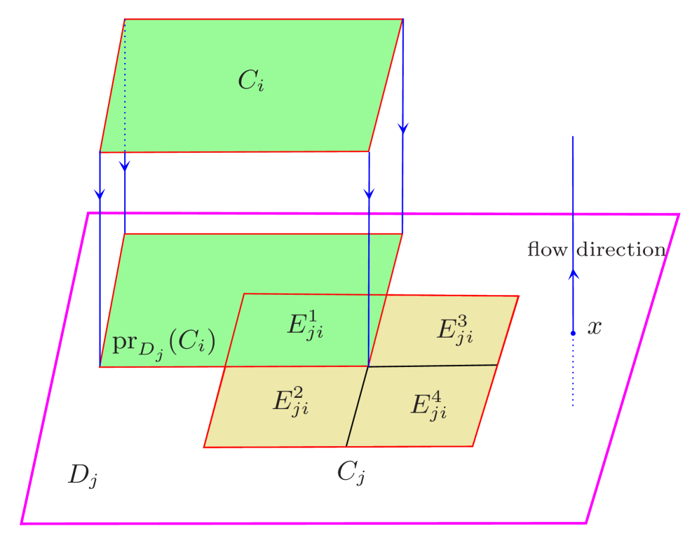
It is clear that $E_{ji}$ is a rectangle having non-empty interior and we see that

$$E_{ji} =\{x\in C_{j}:x={\rm pr}_{D_{j}}(y)\ \mbox{ for some }\ y\in C_{i}\}$$

$$=\{x\in C_{j}:x=\varphi_{\tau}(y)\ \mbox{ for some }\ y\in C_{i}\ \mbox{ and }\ \tau\in[-2\alpha,0]\}$$

$$=\{x\in C_{j}:\varphi_{\upsilon}(x)\in C_{i}\ \mbox{ for some }\ \upsilon\in[0,2\alpha]\}.$$

Figure 8: Projection of $C_{i}$ on $D_{j}$ and $E^{1}_{ij},\dots,E^{4}_{ij}$ partition $C_{j}$

Lemma 6.16.

Pick $z\in{\rm int\,}E_{ji}$. The sets

$$E_{ji}^{1} \ =\ \overline{{\rm int\,}E_{ji}},$$ (6.42)

$$E_{ji}^{2} \ =\ \overline{\{y\in{\rm int\,}C_{j}:\langle z,y\rangle_{C_{j}}\in{\rm int\,}E_{ji},\langle y,z\rangle_{C_{j}}\notin E_{ji}\}},$$ (6.43)

$$E_{ji}^{3} \ =\ \overline{\{y\in{\rm int\,}C_{j}:\langle z,y\rangle_{C_{j}}\notin E_{ji},\langle y,z\rangle_{C_{j}}\in{\rm int\,}E_{ji}\}},$$ (6.44)

$$E_{ji}^{4} \ =\ \overline{\{y\in{\rm int\,}C_{j}:\langle z,y\rangle_{C_{j}}\notin E_{ji},\langle y,z\rangle_{C_{j}}\notin E_{ji}\}}.$$ (6.45)

are rectangles intersecting only in their boundaries.

Proof.

Since $C_{i}$ and $C_{j}$ are rectangles, it follows that $E_{ji}^{1}$ is a rectangle by Remark 4.8. Denote by $G_{ji}^{2}$ the set under the closure symbol in (6.43). For any $y_{1},y_{2}\in G_{ji}^{2}$, we have $y_{1},y_{2}\in{\rm int\,}C_{j}$ and hence $\langle y_{1},y_{2}\rangle\in{\rm int\,}C_{j}$. Furthermore, $\langle z,y\rangle_{C_{j}}=\langle z,\langle y_{1},y_{2}\rangle_{C_{j}}\rangle_{C_{j}}=\langle z,y_{2}\rangle_{C_{j}}\in{\rm int\,}E_{ji}$, owing to $y_{2}\in G_{ij}^{2}$. Also, $\langle y,z\rangle_{C_{j}}=\langle\langle y_{1},y_{2}\rangle_{C_{j}},z\rangle_{C_{j}}=\langle y_{1},z\rangle_{C_{j}}\notin{\rm int\,}E_{ji}$ due to $y_{1}\in G_{ij}^{2}$. Therefore $y=\langle y_{1},y_{2}\rangle_{C_{j}}\in G_{ji}^{2}$. Since $\langle\cdot,\cdot\rangle_{C_{j}}$ is continuous on $C_{j}\times C_{j}$, we deduce that $E_{ij}^{2}$ is a rectangle. Analogously, $E_{ij}^{3},E_{ij}^{4}$ are rectangles.

In addition,

$$C_{j}=E_{ji}^{1}\cup E_{ji}^{2}\cup E_{ji}^{3}\cup E_{ji}^{4}.$$

As ${\rm int\,}E_{ji},G_{ji}^{2},G_{ji}^{3},G_{ji}^{4}$ are pairwise disjoint, $E_{ji}^{1},E_{ji}^{2},E_{ji}^{3},E_{ji}^{4}$ intersect only in their boundaries; See Figure 8 for an illustration. ∎

Lemma 6.17.

The sets $F_{j}^{a(i)}:=\overline{\bigcap_{i\in I_{j}}{\rm int\,}{E_{ji}^{a(i)}}},a(i):I_{j}\to\{1,2,3,4\}$ are rectangles and create a cover of $C_{j}$. Furthermore, elements in

$${\mathfrak{C}}_{j}=\{F_{j}^{a(i)},a(i):I_{j}\to\{1,2,3,4\}\}$$

intersect only in their boundary, and

$$U_{j}=\bigcup_{E\in{\mathfrak{C}_{j}}}{{\rm int\,}E}$$

is an open dense subset of $C_{j}$.

Proof.

By Lemma 6.16, $E_{ji}^{a(i)}$ are rectangles, so are $F_{j}^{a(i)}$ by Remark 4.8 and it is clear that they are a cover of $C_{j}$. The last assertion is obvious. ∎

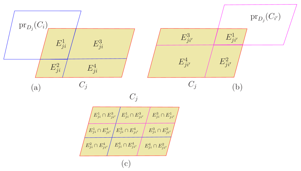
Figure 9: For $I_{j}=\{i,i^{\prime}\}$: projections of $C_{i}$ and $C_{i^{\prime}}$ to $D_{j}$ create partitions of $C_{j}$ in (a) and (b); the set ${\mathfrak{C}_{j}}$ consists of nine sets in (c).

Denote by ${\mathcal{P}}_{\mathscr{C}}$ the Poincaré map for proper family ${\mathscr{C}}=\{C_{1},\dots,C_{n}\}$. For a positive integer $N$, we define

$${\cal C}_{N}=\big{\{}x\in C_{1}\cup\dots\cup C_{n}:{\mathcal{P}}_{\mathscr{C}}^{k}(x)\in\bigcup_{j=1}^{n}U_{j}\quad\mbox{for all}\quad k=1,\dots,N\big{\}}$$ (6.46)

and an equivalence relation on ${\cal C}_{N}$ as follows. For $x,y\in{\cal C}_{N}$, the relation $x\overset{N}{\sim}y$ means that, for every $k\in\{1,\dots,N\}$, ${\mathcal{P}}_{\mathscr{C}}^{k}(x)$ and ${\mathcal{P}}_{\mathscr{C}}^{k}(y)$ not only lie the same $C_{j_{k}}\in{\mathscr{C}}$ but also the same member $F^{a(i)}_{j_{k}}$ of ${\mathfrak{C}}_{j_{k}}$ for some $j_{k}\in\{1,\dots,n\}$. Let $G_{1},\dots,G_{m}$ denote the equivalence classes. Since $N$ is finite and there are finitely many $C_{j}$ and finitely many members in ${\mathfrak{C}}_{j}$, it follows that $m=m(N)$ is finite.

Lemma 6.18.

The sets $\overline{G}_{1},\dots,\overline{G}_{m}$ are rectangles in $X$.

Proof.

We follow the proof of Lemma 7.5 in [6]. For $p\in\{1,\dots,m\}$ fixed, it is enough to verify that if $x,y\in C_{j_{0}},x,y\in G_{p}$, then $z=\langle x,y\rangle_{C_{j_{0}}}\in G_{p}$. Since $G_{p}$ is an equivalence class, in order to achieve $z\in{G}_{p}$, we must show that $x\overset{N}{\sim}z$ or $y\overset{N}{\sim}z$. This means that for each $k\in\{1,\dots,N\}$, ${\mathcal{P}}_{\mathscr{C}}^{k}(x),{\mathcal{P}}_{\mathscr{C}}^{k}(y)$ and ${\mathcal{P}}_{\mathscr{C}}^{k}(z)$ belong to the same $C_{j_{k}}$ for some $j_{k}\in\{1,\dots,n\}$ and the same member of ${\mathfrak{C}}_{j_{k}}$. This is clear for $k=0$ since $C_{j_{0}}$ and $F_{j_{0}}^{a(i)}$ are rectangles. Suppose on the contrary that it is true for all $0\leq k<k^{\prime}$ but not for some $k^{\prime}\leq N$. Then ${\mathcal{P}}_{\mathscr{C}}^{k^{\prime}-1}(x),\,{\mathcal{P}}_{\mathscr{C}}^{k^{\prime}-1}(y)$ and ${\mathcal{P}}_{\mathscr{C}}^{k^{\prime}-1}(z)$ all lie in some $C_{j}$; ${\mathcal{P}}_{\mathscr{C}}^{k^{\prime}}(x),\,{\mathcal{P}}_{\mathscr{C}}^{k^{\prime}}(y)$ lie in some $C_{i^{\prime}}$ but ${\mathcal{P}}_{\mathscr{C}}^{k^{\prime}}(z)$ lies in a $C_{i}\neq C_{i^{\prime}}$. Then by the definition of $I_{j}$ (see (6.40)), $i^{\prime},i\in I_{j}$ and $i^{\prime}\neq i$. It follows from Lemma 6.15 that

$$\langle{\mathcal{P}}_{\mathscr{C}}^{k^{\prime}-1}(x),{\mathcal{P}}_{\mathscr{C}}^{k^{\prime}-1}(y)\rangle_{C_{j}}={\mathcal{P}}_{\mathscr{C}}^{k^{\prime}-1}(\langle x,y\rangle_{C_{j_{0}}})={\mathcal{P}}_{\mathscr{C}}^{k^{\prime}-1}(z).$$ (6.47)

Recall that ${\mathcal{P}}_{\mathscr{C}}^{k^{\prime}-1}(x)$ and ${\mathcal{P}}_{\mathscr{C}}^{k^{\prime}-1}(y)$ lie in the same member of ${\mathfrak{C}}_{j}$ and each member of ${\mathfrak{C}}_{j}$ is a rectangle. It follows from (6.47) that ${\mathcal{P}}_{\mathscr{C}}^{k^{\prime}-1}(z)$ lies in that member too. Note that $z^{\prime}:={\mathcal{P}}_{\mathscr{C}}^{k^{\prime}-1}(z)\in C_{j}\cap{\rm pr}_{D_{j}}(C_{i})=E_{j{i}}$, which is due to $z^{\prime}\in C_{j}$ and ${\mathcal{P}}_{\mathscr{C}}(z^{\prime})\in C_{i}$. Then $z^{\prime}\in E_{ji}^{1}$ implies that $x^{\prime}={\mathcal{P}}_{\mathscr{C}}^{k^{\prime}-1}(x)\in E_{ji}^{1}$, owing to that both $x^{\prime}$ and $z^{\prime}$ lie in the same member of ${\mathfrak{C}}_{j}$. This yields $\varphi_{\tau}(x^{\prime})\in C_{i}$ for some $0<\tau\leq 2\alpha$. Since ${\mathcal{P}}_{\mathscr{C}}(x^{\prime})={\mathcal{P}}_{\mathscr{C}}^{k^{\prime}}(x)\in C_{i^{\prime}}$, there is an $s$ with $0<s<\tau$ so that $\varphi_{s}(x^{\prime})\in C_{i^{\prime}}$, and hence

$$\varphi_{\tau}(x^{\prime})=\varphi_{\tau-s}(\varphi_{s}(x^{\prime}))\in C_{i}\cap\varphi_{[0,2\alpha]}(C_{i^{\prime}})\subset D_{i}\cap\varphi_{[0,2\alpha]}(D_{i^{\prime}}).$$ (6.48)

On the other hand, $x^{\prime}\in E_{{j}i^{\prime}}^{1}$ yields $z^{\prime}\in E_{ji^{\prime}}^{1}$. There is $0<\tau^{\prime}\leq 2\alpha$ such that $\varphi_{\tau^{\prime}}(z^{\prime})\in C_{i^{\prime}}$. Since ${\mathcal{P}}_{\mathscr{C}}(z^{\prime})\in C_{i}$, it follows that $\varphi_{s^{\prime}}(z^{\prime})\in C_{i}$ for some $0<s^{\prime}<\tau^{\prime}$. As a consequence,

$$\varphi_{\tau^{\prime}}(z^{\prime})=\varphi_{\tau^{\prime}-s^{\prime}}(\varphi_{s^{\prime}}(z^{\prime}))\in C_{i^{\prime}}\cap\varphi_{[0,2\alpha]}(C_{i})\subset D_{i^{\prime}}\cap\varphi_{[0,2\alpha]}(D_{i}),$$

which is impossible due to (6.48) and Condition (c) in Theorem 6.9. Therefore, ${\mathcal{P}}_{\mathscr{C}}^{k}(z)$ lies in the same $C_{j_{k}}$ as ${\mathcal{P}}_{\mathscr{C}}^{k}(x)$ and ${\mathcal{P}}_{\mathscr{C}}^{k}(y)$ for $0\leq k\leq N$. In addition, it follows from Lemma 6.15 that

$${\mathcal{P}}_{\mathscr{C}}^{k}(z)=\langle{\mathcal{P}}_{\mathscr{C}}^{k}(x),{\mathcal{P}}_{\mathscr{C}}^{k}(y)\rangle_{C_{j_{k}}}.$$

Since for each $k\in\{1,\dots,n\}$, ${\mathcal{P}}_{\mathscr{C}}^{k}(x)$ and ${\mathcal{P}}_{\mathscr{C}}^{k}(y)$ lie in the same member of ${\mathfrak{C}}_{j}$ and each member is a rectangle, ${\mathcal{P}}_{\mathscr{C}}^{k}(z)$ must lie in that member too. We have shown that if $x,y\in G_{p}$, then $\langle x,y\rangle\in G_{p}$, which implies that $\overline{G}_{p}$ is a rectangle.

∎

Let $\tau_{1},\dots,\tau_{m}$ be so small distinct numbers that $\varphi_{\tau_{1}}(\overline{G}_{1}),\dots,\varphi_{\tau_{m}}(\overline{G}_{m})$ are pairwise disjoint. Using Lemma 6.18, $M_{p}:=\varphi_{\tau_{p}}(\overline{G}_{p}),p=1,\dots,m$ are rectangles. We are going to show that

$${\mathscr{M}}_{N}=\{M_{1},\dots,M_{m(N)}\}$$

is a Markov partition.

For any $p\in\{1,\dots,N\}$, there is $i=i(q)\in\{1,\dots,n\}$ such that $G_{p}\subset C_{i}\subset D_{i}$. Write $\widehat{D}_{p}=\varphi_{\tau_{p}}(D_{i})$ to have $M_{p}\subset\widehat{D}_{p}$. By Condition (c) in Theorem 6.9, if $i\neq j$, then at least one of the sets $\widehat{D}_{i}\cap\varphi_{[0,2\alpha]}(\widehat{D}_{j})$ and $\widehat{D}_{j}\cap\varphi_{[0,2\alpha]}(\widehat{D}_{i})$ is empty. Furthermore, $X=\bigcup_{i=1}^{m}\varphi_{[-\alpha,0]}(C_{i})$ implies that $X=\bigcup_{j=1}^{m}\varphi_{[-2\alpha,0]}(M_{j})$. It follows that ${\mathscr{M}}_{N}$ is a proper family of size $2\alpha$.

The final lemma below proves Theorem 6.8.

Lemma 6.19.

For $N>\frac{L}{2\alpha}$, ${\mathscr{M}}_{N}$ is a Markov partition of time $2\alpha$.

Proof.

We only need to show that ${\mathscr{M}}_{N}$ satisfies the Markov property; see Definition 6.4. Denote by ${\mathcal{P}}_{\mathscr{M}}$ the corresponding return map of ${\mathscr{M}}_{N}$ and

$${\cal M}_{N}^{*}=\{x\in M_{1}\cup\cdots\cup M_{N}\,:\,{\mathcal{P}}_{\mathscr{M}}^{k}(x)\in{\rm int\,}M_{1}\cup\dots\cup{\rm int\,}M_{N}\ \mbox{for all}\ k\in\mathbb{Z}\}.$$

We only prove $(M_{s})$. Recall

$$U(M_{p},M_{q})=\overline{\{z\in{\mathcal{M}}_{N}^{*},z\in M_{p},{\mathcal{P}}_{\mathscr{M}}(z)\in M_{q}\}}.$$

We must show that $W^{s}(x^{\prime},M_{p})\subset U(M_{p},M_{q})$ for $x^{\prime}\in U(M_{p},M_{q})$. Since $U(M_{p},M_{q})$ is closed, $U(M_{p},M_{q})\cap{\cal M}_{N}^{*}$ is dense in $U(M_{p},M_{q})$, and $W^{s}(x^{\prime},M_{p})$ varies continuously with $x^{\prime}$, it is enough to show the inclusion for $x^{\prime}\in U(M_{p},M_{q})\cap{\mathcal{M}}^{*}_{N}$. Also, due to $W^{s}(x^{\prime},M_{p})\cap\varphi_{\tau_{p}}(G_{p})$ is dense in $W^{s}(x^{\prime},M_{p})$, it remains to show $y^{\prime}\in U(M_{p},M_{q})$ for $y^{\prime}=\varphi_{\tau_{p}}(y)$ with $y\in W^{s}(x,\overline{G}_{p})\cap G_{p}$; here $x^{\prime}=\varphi_{\tau_{p}}(x)$. It is enough to show that ${\mathcal{P}}_{\mathscr{C}}(y)\in W^{s}({\mathcal{P}}_{\mathscr{C}}(x),G_{q})$.

Let

$${\mathcal{P}}_{\mathscr{C}}^{k}(x)\in C_{j_{k}}\quad\mbox{for}\quad 1\leq k\leq N.$$

Since $x\overset{N}{\sim}y$, $x_{k}:={\mathcal{P}}_{\mathscr{C}}^{k}(x)$ and $y_{k}:={\mathcal{P}}_{\mathscr{C}}^{k}(y)$ are in the same $C_{j_{k}}$ and in the same member of ${\mathfrak{C}}_{j_{k}}$ for all $0\leq k\leq N$. Due to $y\in W^{s}(x,G_{p})$, $y=\langle x,z\rangle_{G_{p}}$ for some $z\in G_{p}$. We have $x,y,z\in C_{j_{0}}$ and ${\mathcal{P}}_{\mathscr{C}}(x),{\mathcal{P}}_{\mathscr{C}}(y),{\mathcal{P}}_{\mathscr{C}}(z)\in C_{j_{1}}$. Apply Lemma 6.14 to have ${\mathcal{P}}_{\mathscr{C}}(y)=\langle{\mathcal{P}}_{\mathscr{C}}(x),{\mathcal{P}}_{\mathscr{C}}(z)\rangle_{C_{j_{1}}}$ and also ${\mathcal{P}}_{\mathscr{C}}(y)\in W^{s}({\mathcal{P}}_{\mathscr{C}}(x),C_{j_{1}})$. In order to achieve ${\mathcal{P}}_{\mathscr{C}}(y)\in W^{s}({\mathcal{P}}_{\mathscr{C}}(x),G_{q})$, we must show ${\mathcal{P}}_{\mathscr{C}}(y)\in G_{q}$, or equivalently, ${\mathcal{P}}_{\mathscr{C}}(y)\overset{N}{\sim}{\mathcal{P}}_{\mathscr{C}}(x)$. Owing to the fact that $y\overset{N}{\sim}x$, it remains to show ${\mathcal{P}}_{\mathscr{C}}^{N+1}(x)$ and ${\mathcal{P}}_{\mathscr{C}}^{N+1}(y)$ are in the same $C_{j_{N+1}}$ and the same member of ${\mathfrak{C}}_{j_{N+1}}$.

Let

$$x_{N+1}={\mathcal{P}}_{\mathscr{C}}^{N+1}(x)\in C_{j_{N+1}}\quad\mbox{and}\quad y_{N+1}={\rm pr}_{D_{j_{N+1}}}({\mathcal{P}}_{\mathscr{C}}^{N}(y))\in D_{j_{N+1}}.$$

We first claim that

$$y_{N+1}\in W^{s}(x_{N+1},C_{j_{N+1}}).$$ (6.49)

By Lemma 6.12 (a), there is $l\in\{1,\dots,n\}$ such that $\varphi_{-L}(x_{N+1})\in\varphi_{[-\alpha/2,\alpha/2]}(C_{l})$ and

$${\rm pr}_{D_{j_{N+1}}}\varphi_{L}W^{s}({\rm pr}_{D_{l}}\varphi_{-L}(x_{N+1}),C_{l})\subset W^{s}(x_{N+1},C_{j_{N+1}}).$$

For $N>\frac{L}{2\alpha}$, there is a $k\in\{0,\dots,N\}$ such that

$${\rm pr}_{D_{l}}\varphi_{-L}(x_{N+1})={\mathcal{P}}_{\mathscr{C}}^{-k}(x_{N})={\mathcal{P}}_{\mathscr{C}}^{N-k}(x).$$

Furthermore, using $x\overset{N}{\sim}y$ and $y\in W^{s}(x,C_{j_{0}})$, it follows from Lemma 6.15 that ${\mathcal{P}}_{\mathscr{C}}^{-k}(y_{N})\in W^{s}({\mathcal{P}}_{\mathscr{C}}^{-k}(x_{N}),C_{l})$, and also

$$y_{N+1}={\rm pr}_{D_{j_{N+1}}}\varphi_{L}({\mathcal{P}}_{\mathscr{C}}^{-k}(y_{N}))\in W^{s}(x_{N+1},C_{j_{N+1}}),$$

which is (6.49). As a result, $y_{N+1}\in C_{j_{N+1}}$.

Next, we check that $x_{N+1},y_{N+1}$ are in the same member of ${\mathfrak{C}}_{j_{N+1}}$ and also $y_{N+1}={\mathcal{P}}_{\mathscr{C}}(y_{N})$. We first suppose that $x_{N+1},y_{N+1}$ are not in the same member of ${\mathfrak{C}}_{j_{N+1}}$. Then there is some $i\in I_{j_{N+1}}$ for which $x_{N+1}$ and $y_{N+1}$ are in different ${E_{j_{N+1}i}^{a}}$’s; see Figure 9. Taking $z^{\prime}\in{\rm int\,}E_{j_{N+1}i}$, due to (6.49), $\langle y_{N+1},z^{\prime}\rangle_{C_{j_{1}}}=\langle x_{N+1},z^{\prime}\rangle_{C_{j,N+1}}$ by Lemma 4.18. Since $x_{N+1}$ and $y_{N+1}$ are in different $E_{j_{N+1}}^{a}$’s, we may assume that $\hat{x}:=\langle z^{\prime},x_{N+1}\rangle_{C_{j_{N+1}}}\in E_{j_{N+1}i}$ and $\hat{y}:=\langle z^{\prime},y_{N+1}\rangle_{C_{j_{N+1}}}\notin E_{j_{N+1}i}$; see (6.42)-(6.45). Then $\bar{x}={\rm pr}_{D_{i}}(\hat{x})\in C_{i}$ and $\bar{y}={\rm pr}_{D_{i}}(\hat{y})\notin C_{i}$. Let $y_{N+1}^{\prime}={\rm pr}_{D_{i}}(y_{N+1})$ and $x_{N+1}^{\prime}={\rm pr}_{D_{i}}(x_{N+1})$. Using Lemma 6.12 (a), there is $s\in\{1,\dots,n\}$ so that $\varphi_{-L}(\bar{x})\in\varphi_{[-\alpha/2,\alpha/2]}(C_{s})$ and

$${\rm pr}_{D_{i}}\varphi_{L}W^{s}({\rm pr}_{D_{s}}\varphi_{-L}(\bar{x}),C_{s})\subset W^{s}({\rm pr}_{D_{i}}(\bar{x}),C_{i}).$$ (6.50)

Furthermore, due to $N>\frac{L}{2\alpha}$, there is $k^{\prime}\in\{0,\dots,N\}$ such that ${\mathcal{P}}_{\mathscr{C}}^{N-k^{\prime}}(x)={\mathcal{P}}_{\mathscr{C}}^{-k^{\prime}}(x_{N+1})={\rm pr}_{D_{s}}\varphi_{-L}(x_{N+1}^{\prime})\in C_{s}$. Also ${\mathcal{P}}_{\mathscr{C}}^{N-k^{\prime}}(y)={\mathcal{P}}_{\mathscr{C}}^{-k^{\prime}}(y_{N})={\mathcal{P}}_{\mathscr{C}}^{-k^{\prime}}(y_{N})\in C_{s}$ since $y\overset{{}_{N}}{\sim}x$. Owing to

$$\hat{y}=\langle z^{\prime},y_{N+1}\rangle_{D_{j_{N+1}}}=\langle\langle z^{\prime},x_{N+1}\rangle_{D_{j_{N+1}}},y_{N+1}\rangle_{D_{j_{N+1}}}=\langle\hat{x},y_{N+1}\rangle_{D_{j_{N+1}}},$$

we get

$$\bar{y}={\rm pr}_{D_{i}}(\hat{y})=\langle{\rm pr}_{D_{i}}(\hat{x}),{\rm pr}_{D_{i}}(y_{N+1})\rangle_{D_{i}}=\langle\bar{x},y^{\prime}_{N+1}\rangle_{D_{i}}$$

by Lemma 5.3. Also, apply Lemma 5.3 again to obtain

$${\rm pr}_{D_{s}}\varphi_{-L}(\bar{y})=\ \langle{\rm pr}_{D_{s}}\varphi_{-L}(\bar{x}),{\rm pr}_{D_{s}}\varphi_{-L}(y^{\prime}_{N+1})\rangle_{D_{s}}$$

$$=\ \langle{\rm pr}_{D_{s}}\varphi_{-L}(\bar{x}),{\mathcal{P}}_{\mathscr{C}}^{-k^{\prime}}(y_{N})\rangle_{C_{s}}\in W^{s}({\rm pr}_{D_{s}}\varphi_{-L}(\bar{x}),C_{s}).$$

It follows from (6.50) that

$$\bar{y}={\rm pr}_{D_{i}}\varphi_{L}({\rm pr}_{D_{s}}\varphi_{-L}(\bar{y}))\in W^{s}(\bar{x},C_{i})\subset C_{i},$$

which contradicts $\bar{y}\notin C_{i}$ and hence $x_{N+1},y_{N+1}$ are in the same member of ${\mathfrak{C}}_{j_{N+1}}$.

Next, we verify that $y_{N+1}={\mathcal{P}}_{\mathscr{C}}(y_{N})$. Suppose on the contrary that ${\mathcal{P}}_{\mathscr{C}}(y_{N})=\bar{y}_{N+1}\in C_{k}$ for some $k\neq j_{N+1}$. Then $y_{N}\in E_{j_{N}k}$ implies that $x_{N}\in E_{j_{N}k}$ since $x_{N},y_{N}$ belong to the same member of ${\mathfrak{C}}_{j_{N}}$. There is $\tau\in(t(x_{N}),2\alpha]$ such that $\varphi_{\tau}(x_{N})\in C_{k}$. This implies

$$\varphi_{\tau}(x_{N})=\varphi_{\tau-t(x_{N})}(x_{N+1})\in C_{k}\cap\varphi_{[0,2\alpha]}(C_{j_{N+1}})\subset D_{k}\cap\varphi_{[0,2\alpha]}(D_{j_{N+1}}).$$ (6.51)

On the other hand, $y_{N+1}=\varphi_{s}(y_{N})\in D_{j_{N+1}}$ for some $s\in(0,2\alpha]$ and $\bar{y}_{N+1}=\varphi_{t(y_{N})}(y_{N})\in C_{k}$ with $0<t(y_{N})<s$. Then

$$y_{N+1}=\varphi_{s}(y_{N})=\varphi_{s-t(y_{N})}(\bar{y}_{N+1})\in D_{j_{N+1}}\cap\varphi_{[0,2\alpha]}(D_{k}),$$ (6.52)

which is impossible due to (6.51) and Condition (e) in Theorem 6.9. Therefore, $y_{N+1}={\mathcal{P}}_{\mathscr{C}}(y_{N})$ and so $y_{1}\overset{N}{\sim}x_{1}$. To summarize, we have proved that ${\mathcal{P}}_{\mathscr{C}}(y)\in G_{q}$ as well as $y_{1}\in W^{s}(x_{1},G_{q})$. This completes the proof of $(M_{s})$. The proof of $(M_{u})$ is analogous.

∎

Acknowledgments: The author thanks Prof. Markus Kunze for hospitality during his stay at Cologne University. A part of this work was done while the author was working at Vietnam Institute for Advanced Study in Mathematics (VIASM). He would like to thank VIASM for its wonderful working condition. This work is supported by Vietnam’s National Foundation for Science and Technology Development (Grant No. 101.02-2020.21).

References

[1]Adler R. & Weiss B.: Entropy, a complete metric invariant for automorphisms of the torus, Proc. Nat. Aead. Sci. U.S.A.57 (1967), 1573-1576.
[2]Bedford T., Keane M. & Series C. (Eds.): Ergodic Theory, Symbolic Dynamics and Hyperbolic Spaces,
Oxford University Press, Oxford 1991.
[3]Bieder K.:Partner Orbits in Hyperbolic Dynamics, PhD thesis, Ruhr Universität Bochum 2015.
[4]Bowen R.:
Markov partitions for Axiom A diffeomorphisms, Amer. J. Math. 92 (1970), 725-747.
[5]Bowen R.: Periodic orbits for hyperbolic flows,
Amer. J. Math.94(1) (1972), 1-30.
[6]Bowen R.: Symbolic dynamics for hyperbolic flows,
Amer. J. Math.95(2) (1973), 429-460.
[7]Bowen R. & Walters P.: Expansive one-parameter flows,
J. Differential Equations12 (1972), 180-193.
[8]Einsiedler M. & Ward T.: Ergodic Theory with a View
towards Number Theory, Springer, Berlin-New York 2011.
[9]Huynh H.: Partner orbits and action differences on compact factors of the hyperbolic plane. II: Higher-order encounters, Physica D314 (2016), 35-53.
[10]Huynh H.: Expansiveness for the geodesic and horocycle flows
on compact Riemann surfaces of constant negative curvature, J. Math. Anal. Appl.480(2) (2019), 123425.
[11]Huynh H. & Kunze M.: Partner orbits and action differences on compact factors of the hyperbolic plane. I: Sieber-Richter pairs, Nonlinearity 28 (2015), 593-623.
[12]Katok A. & Hasselblatt B.: Introduction to the Modern Theory
of Dynamical Systems, Cambridge University Press, Cambridge-New York 1995.
[13]Lind D. & Marcus B.:An Introduction to Symbolic Dynamics and Coding,
Cambridge University Press 1995.
[14]Pollicott M.: Symbolic dynamics for Smale flows,
Amer. J. Math.109(1) (1987), 183-200.
[15]Pollicott M.: Symbolic dynamics and geodesic flows, Séminaire de théorie spectrale et géomtrie10 (1991-1992), 109-129.
[16]Pollicott M.:
A symbolic proof of a theorem of Margulis on geodesic arcs on negatively curved
manifolds, Amer. J. Math.117(2) (1995), 289-305.
[17]Pollicott M. & Sharp R.: Error terms for growth functions on negatively curved surfaces. Amer. J. Math.120 (1998), 1019-1042.
[18]Pollicott M. & Sharp R.: Error terms for closed orbits of hyperbolic flows,
Ergodic Theory Dyn. Syst.21 (2001), 545-562.
[19]Pollicott M. & Sharp R.: Correlations for pairs of closed geodesics,
Invent. Math.163 (2006), 1-24.
[20]Pollicott M. & Yuri M.:Dynamical Systems and Ergodic Theory, London Mathematical Society Student Texts 40, Cambridge University Press 1998.
[21]Ratner M.: Markov partitions for -flows on 3-dimensional manifolds,
Mat. Zametki6 (1969), 693-704.
[22]Ratner M.: Markov partitions for Anosov flows on -dimensional manifolds,
Isr. J. Math.15 (1973), 92-114.
[23]Ratcliff J.G.: Foundations of Hyperbolic Manifolds,
2nd edition, Springer, Berlin-Heidelberg-New York 2006.