Identifying Peer Influence in Therapeutic Communities

Abstract

We investigate if there is a peer influence or role model effect on successful graduation from Therapeutic Communities (TCs). We analyze anonymized individual-level observational data from 3 TCs that kept records of written exchanges of affirmations and corrections among residents, and their precise entry and exit dates. The affirmations allow us to form peer networks, and the entry and exit dates allow us to define a causal effect of interest. We conceptualize the causal role model effect as measuring the difference in the expected outcome of a resident (ego) who can observe one of their social contacts (e.g., peers who gave affirmations), to be successful in graduating before the ego’s exit vs not successfully graduating before the ego’s exit. Since peer influence is usually confounded with unobserved homophily in observational data, we model the network with a latent variable model to estimate homophily and include it in the outcome equation. We provide a theoretical guarantee that the bias of our peer influence estimator decreases with sample size. Our results indicate there is an effect of peers’ graduation on the graduation of residents. The magnitude of peer influence differs based on gender, race, and the definition of the role model effect. A counterfactual exercise quantifies the potential benefits of intervention of assigning a buddy to “at-risk” individuals directly on the treated resident and indirectly on their peers through network propagation.

Keywords: Networks, Peer Influence, Latent Homophily, Causal Inference, Therapeutic Community

1 Introduction

In application problems from social sciences, social work, public health, and economics, a common form of data collected is a network along with node-level responses and attributes. Such node-level attributes might include responses to questions in a survey, behavioral outcomes, economic variables, and health outcomes, among others. A fundamental scientific problem associated with such network-linked data is identifying the peer influence network-connected neighbors exert on each other’s outcomes.

Therapeutic communities (TCs) for substance abuse and criminal behavior are mutual aid-based programs where residents are kept for a fixed amount of time and are expected to graduate successfully at the end of the program. An important question in TCs is whether the propensity of a resident to graduate successfully is causally impacted by the peer influence of successful graduates or role models among their social contacts. This research aims to quantify the causal role model effect in TCs and develop methods to estimate it using individual-level data from 3 TCs in a midwestern city in the United States.

There is more than half a century of research on understanding how the network and the attributes affect each other (Lazer et al.,, 2010; Manski,, 1993; Lazer,, 2001; Shalizi and Thomas,, 2011; Christakis and Fowler,, 2007, 2008; Aral and Nicolaides,, 2017; Cacioppo et al.,, 2009; Marsden and Friedkin,, 1993; Leenders,, 2002). For example, researchers have found evidence of social or peer influence on employee productivity, wages, entrepreneurship (Chan et al.,, 2014; Herbst and Mas,, 2015; Baird et al.,, 2023), school and college achievement (Sacerdote,, 2011), emotions of individuals (Kramer et al.,, 2014; Coviello et al.,, 2014), patterns of exercising (Aral and Nicolaides,, 2017), physical and mental health outcomes (Christakis and Fowler,, 2007; Fowler and Christakis,, 2008). On the other hand, biological and social networks have been demonstrated to display homophily or social selection, whereby individuals who are similar in characteristics tend to be linked in a network (McPherson et al.,, 2001; Lazer et al.,, 2010; Dean et al.,, 2017; Shalizi and Thomas,, 2011; VanderWeele,, 2011).

Estimating causal peer influence has been an active topic of research with advancements in methodologies reported in Manski, (1993); Shalizi and Thomas, (2011); VanderWeele, (2011); VanderWeele and An, (2013); Bramoullé et al., (2009). It has been shown that peer effects can be identified avoiding the reflection problem Manski, (1993) if the social network is more general than just a collection of connected peer groups Bramoullé et al., (2009); Goldsmith-Pinkham and Imbens, (2013). However, a possible confounder is an unobserved variable (latent characteristics) that affects both the response and the selection of network neighbors and therefore creates omitted variable bias. Peer influence cannot generally be separated from this latent homophily, using observational social network data without additional methodology Shalizi and Thomas, (2011).

Peer influence is a core principle in substance abuse treatment, forming basis of mutual aid based programs including 12 Step programs (White and Kurtz,, 2008), recovery housing (Jason et al.,, 2022; Mericle et al.,, 2023) and TCs (Gossop,, 2000). However, quantitative analyses have nearly always failed to distinguish between peer influence and homophily. It is known that people who are successful in recovering from substance abuse are likely to have social networks that include others in recovery (Best,, 2019; Roxburgh et al.,, 2023), but these studies have not distinguished between peer influence and homophily. In the specific case of TCs, there is evidence that program graduates cluster together (Warren et al., 2020b, ), but this analysis also did not distinguish between peer influence and homophily. In a study that analyzed a longitudinal social network of friendship nominations in a TC using a stochastic actor oriented model (Snijders,, 2017), it was found that resident program engagement was correlated with that of peers, but that homophily and not peer influence explained the correlation (Kreager et al.,, 2019). The question of whether peers influence each other in mutual aid-based programs for substance abuse therefore remains unresolved.

Among substance abuse programs that emphasize mutual aid, the most highly structured and professionalized are TCs. They therefore offer unique opportunities for social network analysis aimed at disentangling peer influence from homophily in substance abuse treatment. TCs are residential treatment programs for substance abuse, based on mutual aid between recovering peers. They typically have a maximum time period for treatment (180 days), which, along with the residential nature of the program, ensures a reasonably stable turnover of participants. The clinical process primarily occurs through social learning within the network of peers who are themselves in recovery (Gossop,, 2000; Yates et al.,, 2017). Peers who exemplify recovery and prosocial behavior, and who are most active in helping others, are known as role models (Gossop,, 2000). It is the job of professional staff to encourage recovery supportive interactions between residents, while also demonstrating prosocial behavior in line with TC values (Gossop,, 2000).

Our goal in this paper is to estimate peer influence, separating it from latent homophily in TCs. The data we analyze comes from three 80-bed TC units. One of these is a unit for women and the other 2 are for men. The units are minimum security correctional units for felony offenders. The offenses of the residents include possession of drugs, robbery, burglary, and domestic violence, among others. All units kept records of entry and exit dates of each resident, along with written affirmations and corrections exchanged that form the basis of our social networks. These networks along with the precise entry and exit dates aides us in correctly identifying the role models to estimate the causal parameter of interest.

The learnings from this paper can help TC clinicians to design network interventions that might increase the graduation rate. For example, one can assign a successful “buddy” to the “at-risk” TC residents if network influence meaningfully impacts graduation status. On the contrary, if latent homophily explains the correlation between the graduation status of network-connected neighbors, then such an intervention is less likely to have any positive impact on graduation. Therefore, it is crucial to disentangle the two effects. The same principle applies to a variety of interventions that could be applied in TCs and other mutual aid-based systems that aim at recovery from substance abuse. There is evidence that gratitude practices are of value in building quality of life as well as social networks (Chang et al.,, 2012), but quantifying it will require the ability to parse homophily from peer influence.

Figure 1: Peer Effects in TC

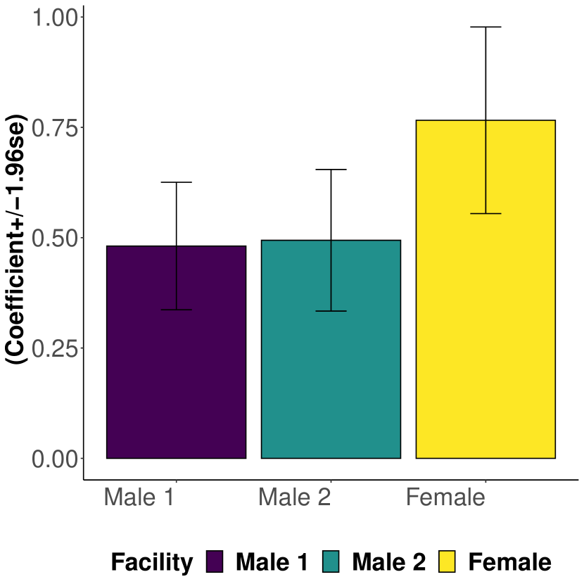
a. Estimated peer effect

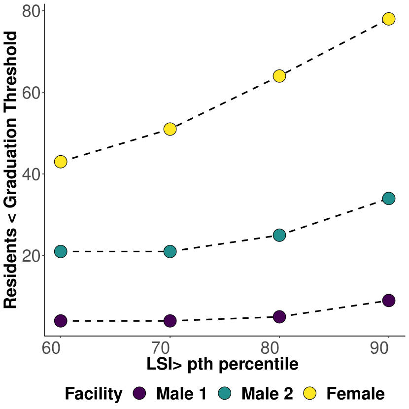
b. Counterfactual Intervention

Notes: Panel (a) displays the estimated causal peer effect from Table 1 (columns 2, 4, and 6) for the three TCs. Panel (b) shows the remaining residents below the graduation threshold post counterfactual interventions for 4 LSI cut-offs.

Recently, several authors have put forth solutions to the problem of separating peer influence from latent homophily, including using latent communities from a stochastic block model (SBM) McFowland III and Shalizi, (2021), and joint modeling an outcome equation and social network formation model Goldsmith-Pinkham and Imbens, (2013); Hsieh and Lee, (2016).

We develop a new method to estimate peer influence adjusting for homophily by combining a latent position random graph model with measurement error models. We model the network with a random dot product graph model (RDPG) and estimate the latent homophily factors from a Spectral Embedding of the Adjacency matrix (ASE). We then include these estimated factors in our peer influence outcome model. A measurement error bias correction procedure is employed while estimating the outcome model.

Our approach improves upon the asymptotic unbiasedness in McFowland III and Shalizi, (2021) by proposing a method for reducing bias in finite samples. Further, we model the network with the RDPG model, which is a latent position model and is more general than the SBM. We provide an expression for the upper bound on the bias as a function of $n$ and model parameters. Our simulation results show the method is effective in providing an estimate of peer influence parameter with low bias both when the network is generated from RDPG as well as the SBM models.

In the context of TCs, we first define a casual “role model influence” parameter with the help of $do-$ interventions Pearl, (2009). We then illustrate the need for adjusting for homophily and correcting for estimation bias of homophily from a network model with the help of a directed acyclic graph (DAG) Pearl, (2009); Hernán and Cole, (2009). We show that the peer influence parameter in our model is equivalent to this role model influence.

Our results show significant peer influence in all TC units (Figure 1). However, there are significant differences in peer effect by gender and race. We see a substantial reduction in peer influence coefficient ($\approx$ 19% drop) once we correct for latent homophily and adjust for the bias in the female correctional unit. On the contrary, we see marginal changes in the two male units. Additionally, the strength of peer influence is at least 30% higher in female unit relative to the male unit. We perform a series of robustness checks to ensure the validity of our results (logistic regression, binarizing network, latent space models and alternative definition of role model effect). We also explore heterogeneous effects by race. For this, we construct separate peer variables for white and non-white peer affirmations and interact these with the white dummy. We find that peer graduation of both races impacts resident’s graduation positively.

Finally, we do a counterfactual analysis to estimate the direct and the cascading effect of a do-intervention of assigning a successful buddy to ”at-risk” residents in the unit. At the beginning of the data collection process, a variable called Level of Service Inventory (LSI) is measured, which is negatively correlated with graduation status (see Figure 5). We use LSI as a proxy for targeting the intervention and compute the overall impact on residents. Panel (b) in Figure 1 suggests that such an intervention can be a useful way for the policymakers to improve graduation from these units as the intervention propagates positively through the network.

2 Methodology

2.1 Data and Statistical Problem Setup

In the TCs the residents dynamically enter and exit the units over time. We observe timestamps for entry and exit for every resident in a TC. The timestamps are critical to our identification. We define a time variable $T$ that takes a value between $\{0,1,...,\tau\}$. Each resident in a TC is denoted by $i\in\{1,2,..,n\}$. The entry and exit dates for the $i$th resident are denoted by $t_{i}^{\text{entry}}\in T$ and $t_{i}^{\text{exit}}\in T$. In our empirical setting, the entry dates spans a period of three years between 2005 and 2008 (see Figure 4). A resident must leave the TC within 180 days, either with a successful graduation or with a failure to graduate.

Let random variable $S_{i}\in\{0,1\}$ denote the final graduation status of individual $i$ within the study population, with the value 1 denoting a successful graduation and 0 a failure to graduate. The goal of this study is to understand the effect of receiving affirmations from peers whom the resident can observe to be successful in graduating on their own graduation. We call this “role model effect”.

Let $A$ denote the $n\times n$ weighted (assumed undirected) adjacency matrix composed of the counts of affirmations, i.e., $A_{ij}$ records the number of affirmations node $i$ has sent (and/or received) to (from) node $j$. Note $i$ can send (receive) affirmations to $j$ only during the time they are both part of the TC. Therefore an entry $A_{ij}$ maybe 0 both because $i$ and $j$ are contemporary and $i$ did not exchange affirmations with $j$ or because they are not contemporary.

We define the variable $Y^{(i)}_{j}$ as the outcome of individual $j$ as observed by $i$ at time $t_{i}^{exit}-1$. If the individual $j$ has already left the TC (whether successful or unsuccessful) by time $t_{i}^{exit}-1$ then $Y^{(i)}_{j}=S_{j}$. Formally, $Y^{(i)}_{j}$ can be defined as follows

$$Y^{(i)}_{j}=\begin{cases}S_{j}&\text{ if }t_{j}^{exit}<t_{i}^{exit}\\ 0&\text{otherwise}\end{cases}$$

2.2 The role model effect estimand

The causal “role model” effect that an individual $i$ receives from an individual $j$ (the role model) can be described as follows.

$$\phi_{ij}=E[S_{i}|A_{ji}>0,do(Y^{(i)}_{j}=1)]-E[S_{i}|A_{ji}>0,do(Y^{(i)}_{j}=0)],$$

where the expectation is taken with respect to the do-interventional distributions of $S_{i}$ Sridhar et al., (2022); Pearl, (2009). The intervention $do(Y^{(i)}_{j}=1)$ can be interpreted as the intervention that $j$ is made to graduate successfully before $i$, while the intervention $do(Y^{(i)}_{j}=0)$ can be interpreted as $j$ is either made to graduate after $i$ or made to fail where $j$ and $i$ exchanged affirmations during their stay in the unit. The expectations in the above definition are marginalizing over all other causes of $S_{i}$, and therefore, the quantity $\phi_{ij}$ can then be thought of as the difference between expectations of successful graduation of $i$ caused by the peer $j$ being a successful graduate, i.e., being a role-model for $i$. The total role model influence of all of $i^{\prime}s$ peers on $i$ can be written as $\phi_{i}=\sum_{j}\phi_{ij}.$

We also define a second causal estimand by changing the definition of the intervention. We only consider the peers who have left the TC before $t_{i}^{exit}$ and define $Y_{j}^{(i)}=S_{j}$ if $t_{j}^{exit}<t_{i}^{exit}$. Then for each individual their potential peer network only consists of individuals who have exited the unit before them. Accordingly we redefine the role model effect $\phi_{ij}^{1}$ as follows:

$$\phi_{ij}^{1}=E[S_{i}|A_{ji}>0,t_{j}^{exit}<t_{i}^{exit},do(S_{j}=1)]\quad-E[S_{i}|A^{1}_{ji}>0,t_{j}^{exit}<t_{i}^{exit},do(S_{j}=0)],$$

For a peer $j$ who has left the TC before the exit date of $i$ (and therefore $i$ can observe their final graduation status), the intervention $do(S_{j}=1)$ is then the $j$th peer is made to graduate successfully and the intervention $do(S_{j}=0)$ is that the peer is made to fail.

We assume that for each unit $i$, there is a $d$ dimensional vector of unobserved latent characteristics $U_{i}$ that affect both the outcome $S_{i}$ and the formation of network $A$. The average role model effect cannot be estimated without additional methodology from our observational data due to the presence of this unobserved homophily. We explain the problem at hand using the following Directed Acyclic Graph (DAG) (McFowland III and Shalizi,, 2021; Hernán and Cole,, 2009; Sridhar et al.,, 2022). The dashed arrows are for unobserved confounders and the solid arrows are for the observed variables.

The direct pathway is $Y_{j}^{i}\rightarrow S_{i}$. This is the causal effect that we are interested in estimating in our setup. However, DAG shows several backdoor pathways which are open.

$$Y_{j}^{i}\dashleftarrow U_{j}\dashrightarrow A_{ji}\rightarrow S_{i}\hskip 2.84544pt\text{and}\hskip 5.69046ptY_{j}^{i}\dashleftarrow U_{j}\dashrightarrow A_{ji}\dashleftarrow U_{i}\dashrightarrow S_{i}$$

We will use the adjacency matrix to estimate a proxy for the unobserved homophily. We denote this proxy variable by $U^{*}$. Below we provide an updated version of DAG. Note that controlling for $U^{*}$ in the regression instead of the true $U$ does not close the backdoor pathways. Therefore, we continue to see bias in the peer influence parameter and cannot capture the causal effect of interest. Nevertheless, we will show that using $U^{*}$ estimated through adjacency spectral embedding of the observed network leads to asymptotically unbiased estimation of peer influence.

Now that we have laid out the core issue about the causal effect, we provide below our structural model. We observe an $n\times p$ matrix $Z$ of measurements of $p$ dimensional covariates at each node. We propose the following data generating model for the expected outcome.

$$E[S_{i}] =\alpha_{0}+\gamma^{T}Z_{i}+\rho\frac{\sum_{j}A_{ji}Y_{j}^{(i)}}{\sum_{j}A_{ji}}+\beta^{T}U_{i}.$$ (2.1)

We will further model the network $A$ as a low-rank model in the next section. The following proposition, which is similar to Proposition 3.1 in Sridhar et al., (2022), shows that if we can identify the parameter $\rho$, then we will be able to identify the role model effect.

Proposition 1.

Assume the data generating model in Equation 2.1 and let $\phi_{i}$ be the role model effect as defined earlier. Then $\phi_{i}=\rho$ for all $i$.

Note that for the second formulation of causal effect $\phi_{ij}^{1}$, when we write the outcome equation, even though we have the same variable $S$ on both left and right-hand side of the equation, due to carefully tracking the exit times of the residents, if $S_{j}$ is in the equation for $S_{i}$, then $S_{i}$ does not appear in the equation for $S_{j}$. This is because $S_{i}$ is observed at time $t_{i}^{\text{exit}}$ and $S_{j}$ happens before $t_{i}^{\text{exit}}-1$.

2.3 Estimating homophily from network model

We develop the methods under a more general setting than our statistical problem such that the methods and the accompanying statistical theory are of independent interest and are applicable more widely to observational data in other contexts of social sciences. We assume we have access to a network encoding relational data among a set of $n$ entities whose adjacency matrix is $A$. Therefore, the element $A_{ij}$ is $1$ if $i$ and $j$ are connected and is $0$ otherwise. The diagonal elements of $A$ are assumed to be $0$. We observe an $n$ dimensional vector $Y$ of univariate responses at the vertices of the network over $t$ time points (with $t\geq 2$, but assumed to be finite). We further observe an $n\times p$ matrix $Z$ of measurements of $p$ dimensional covariates at each node. We assume the following data generating model on the responses:

$$Y_{i,t}=\alpha_{0}+\alpha_{1}Y_{i,(t-1)}+\beta^{T}U_{i}+\rho\frac{\sum_{j}A_{ij}Y_{j,(t-1)}}{\sum_{j}A_{ij}}+\gamma^{T}Z_{i}+V_{i,t},$$ (2.2)

where $V_{i,t}$ are iid random variables with $E[V_{it}]=0$ and $Var[V_{it}]=\sigma^{2}$, and $U$ is a $n\times d$ matrix of latent homophily variables such that each row $U_{i}\in\mathbb{R}^{d}$ of the matrix represents a vector of latent variable values for a node. The parameter $\rho$ is the network peer influence parameter of interest. For any node $i$, the variable $\frac{\sum_{j}A_{ij}Y_{j,(t-1)}}{\sum_{j}A_{ij}}$, measures a weighted average of the responses of the network connected neighbors of $i$ in the previous time point $t-1$. Therefore the above model asserts that outcome of $i$ is a function of weighted average of outcomes of its network connected neighbors in the previous time point, values of the covariates, and a set of latent variables representing unobserved characteristics.

In the outcome model in Equation (2.2), we distinguish between observed covariates $Z$ and unobserved latent variables $U$. While they both can create omitted variable bias for estimating network influence, we can directly control for $Z$ since those variables are observed by the researcher. The variables in $U$ on the other hand, are unobserved confounders that capture several unobserved characteristics of the individuals.

We assume that the selection of network neighbors happens on the basis of homophily or similarity on those unobserved characteristics. Therefore, it is possible to statistically model and extract the latent homophily information from the observed network. More precisely, we model the network to be generated following the Random Dot Product Graph (RDPG) model Sussman et al., (2012); Athreya et al., (2017, 2016); Tang et al., (2018); Rubin-Delanchy et al., (2022) defined as follows. Let $X_{1},\ldots,X_{n}$ be $d$-dimensional vectors of latent positions such that $\|X_{i}\|\leq 1$ and $X_{i}X_{j}^{T}\in[0,1]$ for all $i\neq j$, where $\|.\|$ denotes the vector Euclidean norm. Let $\theta_{n}$ be a scaling factor such that,

$$A\sim Bernoulli(P),\quad P=\theta_{n}XX^{T}.$$ (2.3)

We define the scaled latent positions under this model as $U=(\theta_{n})^{1/2}X$. Clearly, $P=UU^{T}$, and we assume that this $U$ matrix is the same matrix of latent factors as in the outcome equation. The latent factors $U_{i}$ are therefore assumed to be obtained from a $d$ dimensional continuous latent space that satisfies the specified constraint. The scaling factor $\theta_{n}$ controls the sparsity of the resulting network with growing $n$ since the number of edges in the network is $O(n^{2}\theta_{n})$. While $\theta_{n}=O(1)$ will lead to a dense graph, a typical poly-log degree growth rate $\theta_{n}=O(\frac{(\log n)^{c}}{n})$ for some $c>1$ leads to a sparse graph. The RDPG model contains the (positive semideifinite) Stochastic Block Model (SBM), Degree corrected SBM, and mixed membership SBM as special cases Athreya et al., (2017); Rubin-Delanchy et al., (2022). The SBM and its extensions are random graph models with a latent community structure which have been extensively studied in the literature Holland et al., (1983); Rohe et al., (2011); Lei and Rinaldo, (2015); Paul and Chen, (2016); Athreya et al., (2017); Paul et al., (2020).

We assume that the observed nodal covariates $Z_{i}$s do not directly affect the formation of the network, and are therefore not part of the network generating process in Equation (2.3). However, the unobserved latent variables $U_{i}$s are correlated with the observed covariates $Z_{i}$s, the network links $A_{ij}$s, as well as the outcomes of the previous time point $Y_{i,t-1}$. Therefore controlling for $U_{i}$s are important in both determining the network influence as well as the effect of the covariates $Z$. In the RDPG model, since $P_{ij}=U_{i}U_{j}^{T}$, the probability of a connection between nodes $i$ and $j$ depends on their positions $U_{i}$ and $U_{j}$ on the underlying latent space. Nodes which are closer to each other in terms of direction (angular coordinate) are more likely to have a higher dot product and consequently higher propensity to form ties. Therefore the variables $U_{i}$s can capture the unobserved characteristics of the individuals which leads to the selections of network ties.

Since we have used the time lag of the response in the right hand side of the equation, the model can be estimated using Ordinary Least Squares (OLS). It was argued in McFowland III and Shalizi, (2021) that when the latent factors in (2.2) are latent communities from the SBM, then replacing estimated communities in place of the true communities, one can obtain an asymptotically unbiased estimate of $\rho$. Under the more general RDPG model, we provide an explicit asymptotic upper bound on the bias of $\rho$. Further, we propose a method that allows us to obtain a bias-corrected estimator of $\rho$, which we show has some advantages over the estimator in McFowland III and Shalizi, (2021) in finite samples.

We estimate the latent factors through a $d$ dimensional Spectral Embedding of the Adjacency matrix (ASE method). The spectral embedding performs a singular value decomposition (SVD) of the symmetric adjacency matrix $A$. Let $Q_{n\times d}$ be the singular vectors corresponding to the $d$ largest singular values and $\Sigma$ be the diagonal matrix containing those singular values. Then we estimate the latent factor as $\hat{U}=Q\Sigma^{1/2}$. In the second step we use these estimated factors as predictors in the outcome model

$$Y_{i,t}=\alpha_{0}+\alpha_{1}Y_{i,(t-1)}+\beta^{T}\hat{U}_{i}+\rho\frac{\sum_{j}A_{ij}Y_{j,(t-1)}}{\sum_{j}A_{ij}}+\gamma^{T}Z_{i}+V_{i,t},$$ (2.4)

However, similar to the method considered in McFowland III and Shalizi, (2021), replacing $U$ with estimated $\hat{U}$ will lead to bias in the estimates. For example, in the context of linear regression, when regressing $Y$ on just $\hat{U}$ it is well known that due to presence of estimation error in $\hat{U}$, this estimator is biased in finite sample and is biased asymptotically unless the estimation error vanishes BB and Mutton, (1975). The problem is acerbated in the context of the network auto-regressive model as in (2.4) due to various dependencies. However, the following result provides an asymptotic upper bound on the bias. The notation $g(n)=O(f(n))$ for two functions of $n$ means that $g(n)$ and $f(n)$ are of the same asymptotic order, i.e., the ratio $\frac{g(n)}{f(n)}$ is a constant $c$ that does not depend on $n$.

Theorem 1.

Assume the network $A$ is generated according to the $d$-dimensional RDPG model with parameter $\theta_{n},X$ as described above. Let $\hat{U}$ be the estimated latent factor matrix from Adjacency Spectral Embedding (ASE) method. Further assume that $n\theta_{n}=\omega(\log n)^{4c}$ for some $c>1$ and let $c^{\prime}>0$ be another constant. Then the bias in the estimate $\hat{\rho}_{n}$ is given by

$$E[\hat{\rho}_{n}-\rho|A]=O\left(\frac{(\log n)^{2c}}{n\theta_{n}}+\frac{1}{n^{c^{\prime}}}+\frac{(\log n)^{c}}{n^{c}(n\theta_{n})^{1/2}}\right).$$

Theorem 1 provides an asymptotic upper bound on the bias of the least squares estimator. Clearly, the bias decreases with increasing $n$ and as $n\to\infty$, the bias vanishes. We further note that as the density of the network increases, i.e., $\theta_{n}$ increases, the bias in the OLS estimator decreases. This result can be compared with Theorems 1 and 2 in McFowland III and Shalizi, (2021). In comparison to Theorem 1 of McFowland III and Shalizi, (2021) which was for SBM, this result holds for a more general model and allows for sparsity in the network. In comparison to Theorem 2 of McFowland III and Shalizi, (2021), which showed the asymptotic bias with continuous latent space model converges to 0, this result provides an explicit expression for the asymptotic bias as a function of $n$.

2.4 Bias-corrected estimator

Next, we further construct a bias corrected estimator where the central idea is to correct for the finite sample bias using the corrected score function methodology from the well-developed theory of measurement error models Stefanski, (1985); Stefanski et al., (1985); Schafer, (1987); Nakamura, (1990); Novick and Stefanski, (2002). Let $d_{i}=\sum_{j}A_{ij}$ and $D$ denote the diagonal matrix containing $d_{i}$s as the diagonal elements. Define $L=D^{-1}A$, and define $W=[1_{n}\quad Y_{t-1}\quad LY_{t-1}\quad Z]$ as the matrix collecting all the predictor variables except for $\hat{U}$. Let $\eta=[\alpha_{0},\alpha_{1},\rho,\gamma]$. If it is known that $\hat{U}_{i}=U_{i}+\xi_{i}$ and $Var(\xi_{i})=\Delta_{i}$, i.e., if the error covariance matrices for the different nodes are known, then Nakamura, (1990) provides the following bias-corrected estimator. Define the following quantities.

$$\Omega=\begin{pmatrix}\sum_{i}\Delta_{i}&0\\ 0&0\end{pmatrix},\,M_{WU}=\begin{pmatrix}\hat{U}\\ W\end{pmatrix}\begin{pmatrix}\hat{U}&W\end{pmatrix},\,M_{Y}=\begin{pmatrix}\hat{U}\\ W\end{pmatrix}Y.$$

Then the bias-corrected estimator is :

$$\begin{pmatrix}\hat{\eta}&\hat{\beta}\end{pmatrix}^{T}=(M_{WU}-\Omega)^{-1}M_{Y}.$$

However, in practice, the covariance matrix of the error is unknown. We propose to use the result from Athreya et al., (2016); Tang et al., (2018) on estimates of covariance matrix for a finite number of nodes. Define the second moment matrix $\Delta_{F}=E[X_{1}X_{1}^{T}]$. Then define

$$\Sigma(x)=\Delta_{F}^{-1}(E[\{X_{1}^{T}x(1-\theta_{n}X_{1}^{T}x)\}X_{1}X_{1}^{T}])\Delta_{F}^{-1}.$$

Recall the true latent variable for the $i$th node is given by $U_{i}=\theta_{n}^{1/2}X_{i}$. Then the covariance matrix of the error $\Delta_{i}$ for the $i$th node is given by $\Sigma(X_{i})/n$, where $\Sigma(X_{i})$ is the matrix obtained by replacing $x$ with the true latent position $X_{i}$ in the above function. In practice, to estimate this covariance matrix we propose to replace each of the $X_{i}$s with their estimates $\hat{X}_{i}=(\theta_{n})^{-1/2}\hat{U}_{i}$. The resulting estimate of the covariance matrix for the $i$th node, $\hat{\Delta}_{i}$ is given below:

$$\hat{\Delta}_{i}=\hat{\Delta}_{F}^{-1}(\sum_{j}\hat{U}_{j}^{T}\hat{U}_{i}(1-\hat{U}_{j}^{T}\hat{U}_{i})\hat{U}_{j}\hat{U}_{j}^{T})\hat{\Delta}_{F}^{-1},$$

where $\hat{\Delta}_{F}=\frac{1}{n}\sum_{i}\hat{U}_{i}\hat{U}_{i}^{T}$. In the special case of SBM, the covariance matrix simplifies further. We assume the number of communities is same as the number of dimensions of the latent positions, $d$. Let $B_{k}$ denote the unique row corresponding to the $k$th community and $c_{i}\in\{1,\ldots,d\}$ denotes the community the node $i$ belongs to. Let $\pi_{k}$ denotes the proportion of nodes that belong to community $k$. Then to apply corollary 2.3 of Tang et al., (2018), we compute $\Delta_{F}=E[U_{1}U_{1}^{T}]=\sum_{k=1}^{K}\pi_{k}B_{k}B_{k}^{T}$ and $\Sigma(B_{q})=\Delta_{F}^{-1}(\sum_{k=1}^{K}\pi_{k}B_{k}B_{k}^{T}(B_{q}^{T}B_{k}-(B_{q}^{T}B_{k})^{2}))\Delta_{F}^{-1}$. We propose to estimate $B_{q}$ with its natural estimate $\hat{B}_{q}$ which are the cluster centers, and $\pi_{q}$ with $\hat{\pi}_{q}$ which are the cluster size proportions. Therefore a plug-in estimator for the covariance matrix $\hat{\Delta}_{q}$ for any $\hat{U}_{i}$ whose true community is $q$, is

$$\hat{\Delta}_{q}=\hat{\Delta}_{F}^{-1}(\sum_{k}\hat{\pi}_{q}(\hat{B}_{q}^{T}\hat{B}_{k}-(\hat{B}_{q}^{T}\hat{B}_{k})^{2})\hat{B}_{k}\hat{B}_{k}^{T})\hat{\Delta}_{F}^{-1},$$

where $\hat{\Delta}_{F}=\frac{1}{n}\left(\sum_{k}\hat{\pi}_{k}\hat{B}_{k}\hat{B}_{k}^{T}\right)$. We find in our simulations that this estimate of the covariance matrix works well even when the model is more general than SBM, and we find that in our real data example this estimate gives very similar results as the original estimate.

We also note that the results in Tang et al., (2018); Athreya et al., (2016) hold nodewise and therefore does not hold simultaneously for all $n$ nodes. However, we show in the simulations that our measurement bias correction methods with this estimate of the covariance matrix provides effective bias corrections, especially in small samples. To motivate the bias correction procedure, suppose we have access to the true latent positions for all nodes except for node $i$, i.e., we observe $U_{1},\ldots U_{i-1},U_{i+1},\ldots U_{n}$. For ease of notation, we call these latent position vectors together as $U_{-i}$. For the $i$th node we use our estimate $\hat{U}_{i}$ from the ASE. As described earlier, we can write the linear regression model of interest as $Y=\hat{U}\beta+W\eta+V$, with $E[V]=0$. We have the following theorem.

Theorem 2.

Consider the RDPG model described above with latent positions $U_{1},\ldots,U_{n}$, and the linear regression model with the latent factors as $Y=\hat{U}\beta+W\eta+V$, with $E[V]=0$. Let $U_{-i}$ are known latent positions, and $\hat{U}_{i}$ is estimated from the ASE method. Then the estimator using $U_{-i},\hat{U}_{i}$ and without bias-correction, $\begin{pmatrix}\hat{\eta}&\hat{\beta}\end{pmatrix}^{T,(old)}=(\sum_{j}W_{j}W_{j}^{T}+\sum_{j\neq i}U_{j}U_{j}^{T}+\hat{U}_{i}\hat{U}_{i}^{T})^{-1}(\sum_{j}Y_{j}W_{j}+\sum_{j\neq i}Y_{j}U_{j}+Y_{i}\hat{U}_{i})$ converges in probability to $(E[W_{i}W_{i}^{T}]+E[U_{i}U_{i}^{T}]+\Sigma(U_{i}))^{-1}(E[W_{i}W_{i}^{T}]+E[U_{i}U_{i}^{T}])\begin{pmatrix}\eta_{0}&\beta_{0}\end{pmatrix}^{T}$. However, the bias corrected estimator $\begin{pmatrix}\hat{\eta}&\hat{\beta}\end{pmatrix}^{T,(new)}=(\sum_{j}W_{j}W_{j}^{T}+\sum_{j\neq i}U_{j}U_{j}^{T}+\hat{U}_{i}\hat{U}_{i}^{T}-\Sigma(U_{i}))^{-1}(\sum_{j}Y_{j}W_{j}+\sum_{j\neq i}Y_{j}U_{j}+Y_{i}\hat{U}_{i})$ converges to $\begin{pmatrix}\eta_{0}&\beta_{0}\end{pmatrix}^{T}$.

The above theorem shows that the bias correction procedure converges to the target parameter when only one latent position is taken from the output of the ASE algorithm while the others are known. Our bias correction procedure generalizes this motivation for all nodes.

Finally, we remark that in our model, while $U\beta$ is identifiable, the parameter $\beta$ cannot be identified separately. This is because the latent variable $U$ can be estimated only up to the ambiguity of an orthogonal matrix $R$.

3 Simulation

We perform several simulation studies to compare the bias-corrected estimator using the estimated covariance matrix from ASE with both (1) the estimator without any latent homophily variable and (2) the estimator with latent homophily vector from ASE but not corrected for measurement bias. In all cases, the network $A$ is generated from a specific instance of the RDPG model with 2-dimensional latent homophily variables collected in the matrix $U$. Next we generate the response at the first time point as $Y_{i1}=V_{i1}$, at the second time point as $Y_{i2}=U_{i}\beta+\alpha Y_{i1}+V_{i2}$ and at the third time point as $Y_{i3}=\alpha Y_{i2}+U_{i}\beta+\rho\sum_{j}L_{ij}Y_{j2}+V_{i3}$, with $V_{i1},V_{i2},V_{i3}$ being generated i.i.d from $N(0,1)$ distribution. We set the parameters $\alpha=0.6$ and $\rho=0.3$ and vary different parameters to investigate a variety of simulation setups.

3.1 DCSBM graph with increasing nodes

For this simulation, we generate a network from the Degree-corrected Stochastic Block Model (DCSBM), which is a special case of the RDPG model with the number of nodes increasing from 100 to 800 in increments of 100. Every node has a different latent position under this model. The degree heterogeneity parameters are generated from a log-normal distribution with log mean set at 0 and log SD set at 0.5. The matrix $U$ is formed as $U=\Theta HJ$, where $\Theta$ is the diagonal matrix of degree parameters, $H$ is the community assignment matrix whose $i$th row is such that only one element takes the value of $1$, indicating its community membership and all other elements are 0s, and $J=\begin{pmatrix}0.5&0.1\\ 0.1&0.5\end{pmatrix}$ is a matrix whose rows provide the direction of the cluster centers. The community assignments are generated from a multinomial distribution with equal class probabilities. We form the matrix as $P=UU^{T}$ and scale all elements by a number to make the average density of the graph 0.20. In the outcome model, we set $\beta=(1,3)$. We report the bias and Standard Error (SE) of the bias for the three competing methods in Figure 2 (left). As the figure shows, the estimator without homophily correction remains biased even when the sample size increases, while the bias in the two homophily-corrected estimators decreases as the number of nodes increases. The figure further shows that the proposed measurement error bias-corrected estimator for the peer effect parameter $\rho$ has less bias compared to the estimator with homophily control but no bias correction, especially in small samples. The bias in the parameter estimate goes close to 0 more quickly with the measurement error correction. Therefore, the proposed bias correction methodology works well.

Figure 2: Comparison of estimates of the peer influence parameter $\rho$ when the underlying graph is generated from a DCSBM model with (left) increasing number of nodes, (right) increasing density of the graph

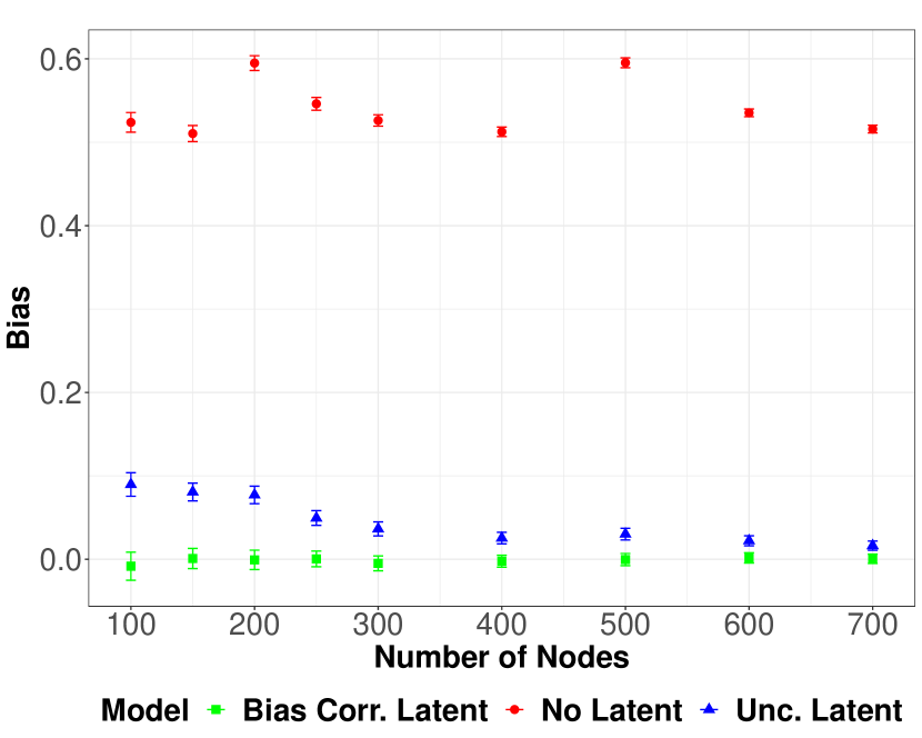
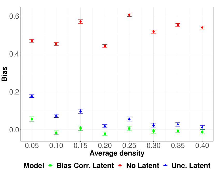
3.2 DCSBM graph with increasing density

Next we again generate the networks from a DCSBM model but increase the average density of the graphs approximately from 0.05 to 0.40, fixing the number of nodes at 200. For this simulation, we set the same $J$ and $\beta$ as the previous simulation, and the parameters in $\Theta$ are generated from the lognormal distribution with the same mean and SD as in the previous simulation. As Figure 2(right) shows the bias-corrected latent factor method outperforms the other two methods. We also see that the bias of both the uncorrected estimator and the bias-corrected decreases with increasing density as predicted by Theorem 1, while the bias of the estimator without latent factors remains high.

3.3 Increasing nodes, SBM underlying graph

Now we consider the case when the data is generated from the stochastic block model. For this purpose, we set the $U$ matrix to a matrix which has 2 columns and 4 rows as $U=\begin{pmatrix}0.7&0.2\\ 0.1&0.6\\ 0.2&0.2\\ 0.5&0.5\\ \end{pmatrix}$. This leads to $d=2$ and the number of communities $K=4$. Figure 3 (left) shows the performance of the estimators with increasing number of nodes when $\beta$ is set to $(1,2)$. As noted in McFowland III and Shalizi, (2021) for the case of SBM, the estimator without homophily correction remains biased even with increasing $n$. We notice that in smaller sample sizes, the bias-corrected estimator improves upon the non bias-corrected estimator substantially.

Figure 3: Comparison of estimates of the peer influence parameter $\rho$ when the underlying graph is generated from a SBM model with (left) increasing number of nodes, (right) when the model with no latent factors has both positive and negative bias.

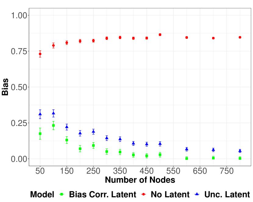
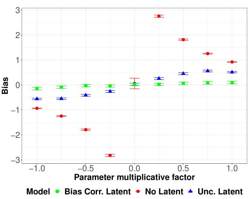
3.4 Negative and positive bias

Next, we design a simulation set-up to test the ability of the bias correction procedure to reduce bias in both positive and negative directions. We set $J$ and $\beta$ as in simulation B, but keep $diag(\Theta)$ as 1 for all nodes for simplicity (therefore making the model SBM). However, the parameter associated with $U$ in the previous time period is changed to $\beta^{\prime}=m\beta$, where $m$ is varied from $-1$ to $1$ in increments of $0.25$. The negative $m$’s are going to create negative bias in the uncorrected estimator. The highest magnitude of the bias is seen at $-0.25$ and $0.25$. In Figure 3(right) we see that the bias-corrected estimator succeeds in correcting bias of the estimator both when the estimator with no latent factor is biased with negative and positive bias.

4 Results

4.1 Data

The data from the 3 TCs spans over three or four years, depending on the unit. We use the data only on those residents for whom we observe non-missing values for outcome, covariates, and if they sent and received affirmations at least once during their time in the TC. The residents entered the unit at different points in time (Panel (a) in Figure 4) and spent varying amounts of time (Boxplot in Panel (b) in Figure 4). The median time of stay for residents in male unit 2 and female unit is 149 and 150 days, respectively, while the same for residents in male unit 1 is considerably lower at 124 days. The participants remain in these units for a maximum of six months. The information on entry and exit dates is critical for estimating the causal role model effect. Also, the residents of the TCs interact only within the TC and there is no interaction across TCs.

Figure 4: Variation in entry dates and time spend with the peers in TCs

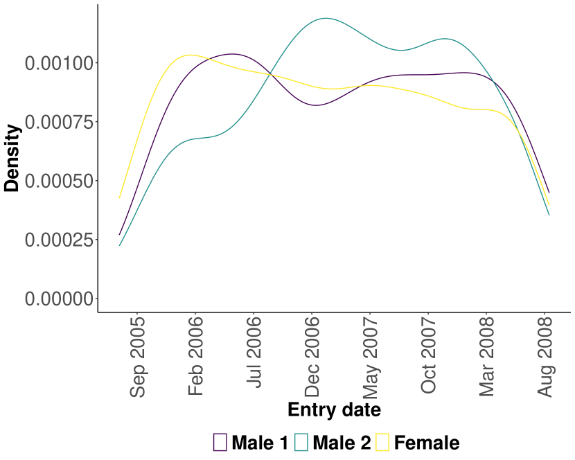
a. Entry Date

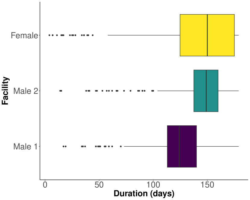
b. Time in TC

The TCs maintained records on socio-demographic characteristics, behavioral aspects, and graduation status of the residents. Moreover, the officials implemented a system of mutual feedback among the residents. This took the form of positive affirmations of prosocial behavior of peers (Campbell et al., (2021); Warren et al., 2021b ; Warren et al., 2021a ; Warren et al., 2020a ). The male units 1 and 2 have about 7400 and 16000 affirmations. The female unit includes a little over 61,000 instances of affirmations over a three-year period. For each of these instances, we observe the anonymized IDs of the sender and the receiver, and the timestamp of the message. In addition, feedback also involved sending written corrections of behavior that contravenes TC norms. In a separate analysis, we explore peer influence that propagates through the corrections network (see section 4.4).

Since the composition of the TC is changing continuously, the interaction networks the residents form evolve dynamically. The outcome variable of interest is the final graduation status, denoted by $S_{i}$. Among the female residents, 79.7% graduated successfully from the TC. In male unit 1, we observe that 88% of the residents graduated successfully during the period of study, and in male unit 2, the corresponding number is 89%. The primary explanatory variable is the weighted average of the graduation status of peers ($\frac{\sum_{j}A_{ij}Y_{j,(t-1)}}{\sum_{j}A_{ij}}$) as observed by resident $i$ just before his/her time of exit. This variable is a function of the affirmations sent and received and the entry and exit dates of $i$ and his/her peers. Using the affirmations data and the time stamps, we can extract all the peers who sent or received affirmations from/to $i$ starting $t_{i}^{\text{entry}}$ to date $t_{i}^{\text{exit}}-1$. In Figure B1 (in SI) we see that residents who graduated (not graduated) had a higher (lower) fraction of peers graduated by time $t_{i}^{\text{exit}}-1$. The correlation is positive but it is likely confounded with unobserved homophily.

Figure 5: LSI and Graduation Status

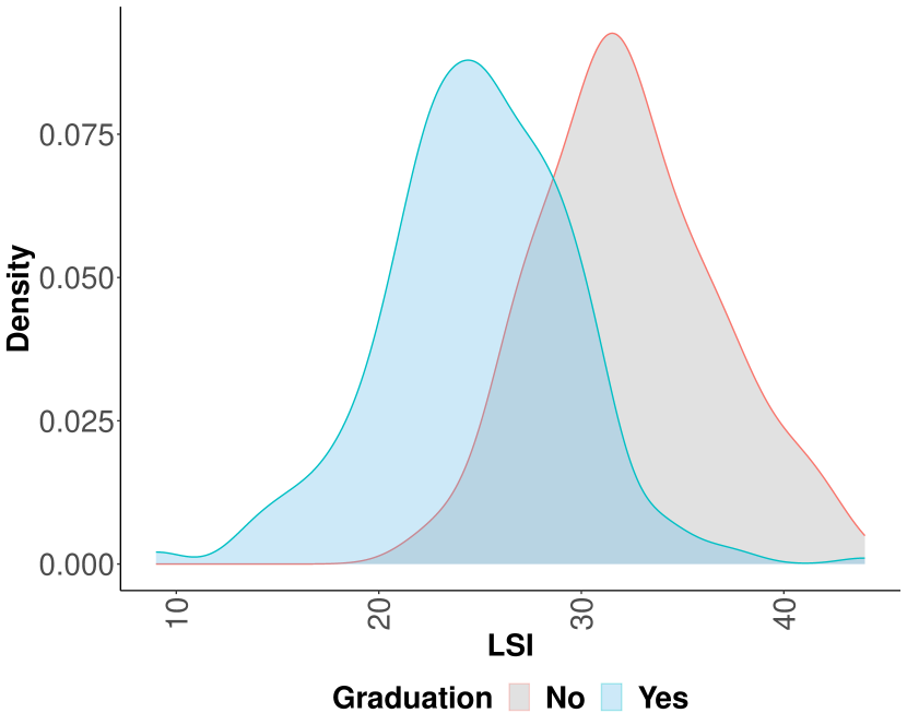
a. Male Unit 1

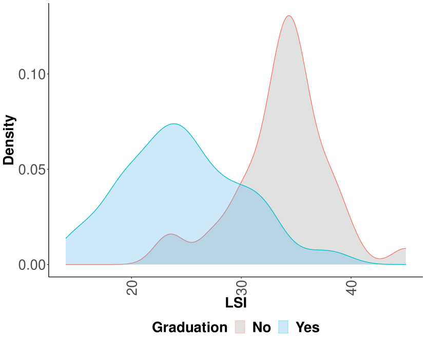
b. Male Unit 2

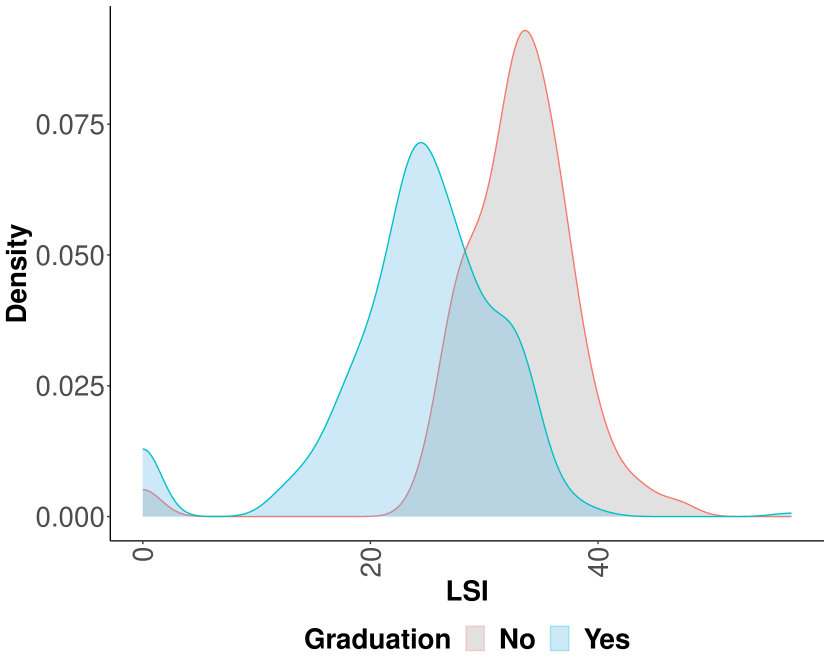
c. Female Unit

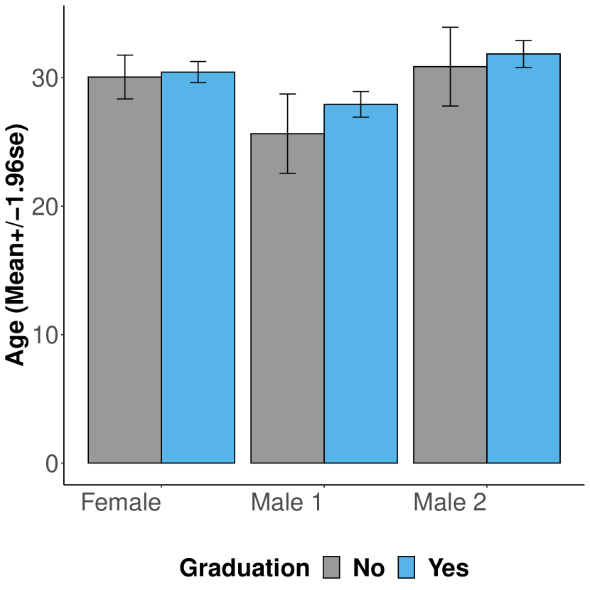
d. Graduation status and age

e. Graduation and Proportion of Blacks

Notes: First row (a,b and c) illustrates the correlation between LSI and $S_{i}$. Panel (d) shows the variation in age by graduation status. Panel (e) shows the proportion of black residents among the residents who were able to successfully graduate and those that did not graduate from the unit. The difference in means for proportion of blacks and the se of the difference is shown at the top of the bar and in parenthesis.

Moreover, we observe a vector of covariates that we control for in our empirical specification. Table B1 (in SI) provides summary statistics. In terms of socio-demographic characteristics, the sample is 80% white in the female unit. The corresponding percentages for the male units 1 and 2 are 47.5% and 77.6% respectively. Age distribution has a mean of 30 years for the female unit, 27.6 years for male unit 1, and 31.7 years for the second male unit. The facility also recorded the LSI (Andrews and Bonta,, 1995) at the time of entry of each resident. The LSI is a standardized instrument that rates the service needs of residents based on a set of factors, such as substance abuse and family relations, which are known to predict criminal recidivism. The average LSI score is slightly over 25 across all 3 units.

We show that these covariates likely have some explanatory power for $S_{i}$. Figure 5 shows the distribution of LSI by $S_{i}$. We see that for all units the distribution of LSI is shifted to the right for the non-graduates relative to the graduates. Next, we show the relationship between age of the residents and the graduation status. We find small differences in the means for age between those who graduated and those who did not graduate from the unit.

Finally, panel (e) in Figure 5 shows the proportion of blacks between the graduates and non-graduates. We see several interesting patterns. First, male unit 2 and female units have a much smaller proportion of black residents than male unit 1. Interestingly, we see large differences in the proportion of blacks among the graduates and non-graduates in these two units. However, this difference is marginal in male unit 1 where there is a balanced proportion of residents by race.

4.2 Peer Influence with Affirmations Network

We provide the results for role model effects in all units. Table 1 has 3 panels, one for each unit. Every panel has two columns. The first column presents the parameter estimates for peer graduation without correcting for homophily. In the second column, we provide the estimates using the estimator developed in this paper, which both corrects for latent homophily and additionally adjusts for bias. The sample sizes are 337 in male unit 1, 339 in male unit 2, and 472 in the female unit.

The estimation for our preferred specification (columns (2), (4) and (6)) are done using the following steps. First, we do SVD of the adjacency matrix of affirmations and obtain $\hat{U}$ as described in the methodology section. The selection of the dimension $d$ is done via cross-validation. We plot the out-of-sample AUC values for $d\in\{1,2,..,20\}$. The AUC rises steeply as we increase $d$ initially but it stabilizes to a high value around or above 0.9 after a few initial points. We select $d$ corresponding to the point where the AUC becomes stable at a large value. Figure B2 (in SI) shows the out-of-sample AUC as we increase $d$. Second, we use these estimated $\hat{U}$ as covariates in our outcome model and correct for the bias arising from using $\hat{U}$ instead of true $U$.

We find a decline in the estimates for peer graduation effect once we correct for homophily and bias. We find the sharpest decline for the female unit ($\approx$ 19%). The changes for male units are marginal. While the impact of peer graduation status is lower with the homophily and bias correction it continues to increase the resident’s graduation substantially. The parameters on peer graduation in columns (2), (4) and (6) are statistically significant in the sense that the 95% confidence intervals around the point estimates do not include the null effects. We find that a 10% increase in the graduation of peers improves a resident’s likelihood of graduating by 4.8-7.7 percentage points (pp).

Table 1: Peer Effects in TC

	Dependent Variable: $S_{i}$
	(1)	(2)	(3)	(4)	(5)	(6)
Variable	OLS	Homophily and Bias Adj.	OLS	Homophily and Bias Adj.	OLS	Homophily and Bias Adj.
	a. Male Unit 1		b. Male Unit 2		c. Female Unit
Peer Grad.	0.483	0.481	0.500	0.494	0.940	0.766
	(0.073)	(0.074)	(0.082)	(0.082)	(0.099)	(0.108)
Age	0.000	0.000	0.000	0.000	0.002	0.000
	(0.002)	(0.002)	(0.002)	(0.002)	(0.002)	(0.002)
White	-0.074	-0.077	0.015	0.019	0.079	0.068
	(0.030)	(0.031)	(0.035)	(0.035)	(0.039)	(0.038)
LSI	-0.028	-0.028	-0.021	-0.021	-0.016	-0.016
	(0.003)	(0.003)	(0.002)	(0.002)	(0.002)	(0.002)
Notes: Standard errors are provided in parenthesis.

As for the other covariates, we find some interesting patterns. Being white lowers graduation in male unit 1 where we observe a better balance of white and black residents (refer to Figure B1). However, in male unit 2 and female unit we see a positive coefficient on white dummy, although the standard errors are large. This specification does not inform us if impact of peer graduation status varies by race. Importantly, we explore whether the racial identity of role models in peer group matter for graduation from the unit in the next specification.

Table 2: Peer Effects and Race (Homophily and Bias Adj.)

	Dependent Variable: $S_{i}$
	(1)	(2)	(3)
Variable	Male Unit 1	Male Unit 2	Female Unit
Peer Grad. (White)	0.225	0.609	0.560
	(0.097)	(0.161)	(0.235)
Peer Grad. (Non-White)	0.194	0.113	0.202
	(0.101)	(0.123)	(0.235)
White	-0.140	0.140	0.064
	(0.071)	(0.080)	(0.092)
Peer Grad. (White) $\times$ White	0.064	-0.195	0.079
	(0.134)	(0.189)	(0.259)
Peer Grad. (Non-White) $\times$ White	0.093	-0.116	-0.069
	(0.141)	(0.137)	(0.254)
Age	0.000	0.000	0.000
	(0.002)	(0.002)	(0.002)
LSI	-0.029	-0.021	-0.016
	(0.003)	(0.002)	(0.002)
Notes: Standard errors are provided in parenthesis. The baseline category is the mean graduation for a non-white resident.

In order to capture the heterogeneous effects of peer graduation status, we modify construction of the peer graduation variable as follows. For each resident $i$, we extract the graduation status of white peers that have left the unit before $i$. Using this subset of peers which is specific to $i$, we calculate the weighted average of graduation status for white peers $(\frac{\sum_{j_{\text{white}}}A_{ij}Y_{j,(t-1)}}{\sum_{j_{\text{white}}}A_{ij}})$. Similarly, we repeat this exercise for non-white peers and construct $(\frac{\sum_{j_{\text{non-white}}}A_{ij}Y_{j,(t-1)}}{\sum_{j_{\text{non-white}}}A_{ij}})$. We use both these peer variables on the RHS and also interact them with the white dummy. Table 2 presents the estimates. The intercept of the regression (not shown) provides us the mean graduation status for the baseline group (non-white residents), while the coefficients for Peer Grad (white) and Peer Grad (Non-white) provide effects of White peers’ graduation and non-white peers’ graduation on non-white residents. Across all 3 units, we find that the peer graduation of both white and non-white residents’ impacts the graduation status positively. However, the standard errors for the coefficient on peer graduation for non-white residents is very high specially in male unit 2 and female unit due to small samples of non-white residents. In the male unit 1, where there is a better balance of white and non-white residents, we see the effects are almost identical. We also do not have enough power to distinguish a differential impact of peer graduation of white on white and peer graduation of non-white on white residents.

4.3 Second Definition of Role Model

In this section, we use the second definition of role models as described in the methodology (Section 2.2). According to the second definition, peer group only consists of those peers who have exited the unit before resident $i^{\prime}s$ exit date. Consequently, resident $i$ observes the final graduation status of these subset of peers. We report the estimates in Table 3. The direction of role model effect continues to be positive and large compared to their standard errors, as seen in Table 1. However, the magnitude of the coefficients drops substantially. This could be because this definition makes the set of peers much smaller than the first definition. Nevertheless, we see a decline in the coefficient on peer graduation status when we control for homophily and adjust for the bias. In line with the observation in Table 1, the drop is large in the female unit (¿ 50%) relative to the two male units.

Table 3: Peer Effects in TC (Second Def. of Role Model)

	Dependent Variable: $S_{i}$
	(1)	(2)	(3)	(4)	(5)	(6)
Variable	OLS	Homophily and Bias Adj.	OLS	Homophily and Bias Adj.	OLS	Homophily and Bias Adj.
	a. Male Unit 1		b. Male Unit 2		c. Female Unit
Peer Grad.	0.288	0.286	0.179	0.172	0.437	0.212
	(0.073)	(0.076)	(0.090)	(0.091)	(0.104)	(0.107)
Age	0.000	0.000	0.000	0.001	0.001	-0.001
	(0.002)	(0.002)	(0.002)	(0.002)	(0.002)	(0.002)
White	-0.045	-0.049	0.016	0.019	0.106	0.083
	(0.031)	(0.032)	(0.037)	(0.037)	(0.042)	(0.040)
LSI	-0.028	-0.029	-0.023	-0.023	-0.019	-0.017
	(0.003)	(0.003)	(0.002)	(0.002)	(0.002)	(0.002)
Notes: Standard errors are provided in parenthesis.

4.4 Corrections Network

So far, we have conducted the analysis of peer effects using the affirmations network. Next, we use the corrections network to estimate peer influence in TCs. A primary difference between the affirmations and the corrections network is that we see residents sent each other many more corrections than affirmations. Consequently, our analysis sample is larger when we use the corrections network than the affirmations network. The sample sizes are 774 in male unit 1, 391 in male unit 2, and 1046 in the female unit. However, the impact of peers who sent affirmations can be different from the ones that sent corrections. Table 4 shows that peer graduation positively impacts the likelihood of graduation from the unit. We find that LSI negatively impacts the propensity to graduate from the unit, which is similar to the coefficients on LSI in Table 1. Lastly, the coefficients on age and white dummy are not statistically significantly different from 0 for most specifications. We also examine heterogeneity by race and it is reported in Table B2 in SI.

Table 4: Peer Effects in TC (Homophily in Corrections Network)

	Dependent Variable: $(S_{i})$
	(1)	(2)	(3)	(4)	(5)	(6)
Variable	OLS	Homophily and Bias Adj.	OLS	Homophily and Bias Adj.	OLS	Homophily and Bias Adj.
	a. Male Unit 1		b. Male Unit 2		c. Female Unit
Peer Grad.	0.359	0.339	0.723	0.722	0.544	0.523
	(0.054)	(0.056)	(0.077)	(0.077)	(0.056)	(0.056)
Age	0.001	0.001	-0.000	-0.001	0.001	0.001
	(0.001)	(0.001)	(0.001)	(0.001)	(0.001)	(0.001)
White	-0.035	-0.035	0.004	0.009	0.071	0.074
	(0.020)	(0.021)	(0.032)	(0.032)	(0.022)	(0.022)
LSI	-0.025	-0.025	-0.023	-0.024	-0.016	-0.016
	(0.002)	(0.002)	(0.002)	(0.002)	(0.001)	(0.001)
Notes: Standard errors are provided in parenthesis. The latent homophily vectors are estimated from the corrections network in these specifications.

4.5 Robustness Checks

In this section, we provide robustness checks for our estimates of peer effects. We begin using a logistic regression instead of a linear model. Note that since our bias-corrected estimator is developed for the linear models, we cannot use it for the logistic regression. However, we can still use the affirmations network to estimate the latent homophily vectors and use them as covariates in a logistic regression outcome model. We call this specification homophily corrected specification. We report the average marginal effects. The marginal effect w.r.t a continuous variable $Z_{k}$ is provided below.

$$\text{ME}_{Z_{k}}=\lim_{\Delta\rightarrow 0}\frac{P(S_{i}=1|Z,Z_{k}+\Delta)-P(S_{i}=1|Z,Z_{k})}{\Delta}$$

The marginal effect would vary for each individual and we compute it for all residents and then take an average to calculate the average marginal effect. In Panel (a) in Table 5, the estimates are in line with our conclusions shown in Table 1.

Table 5: Robustness Checks

	Dependent Variable: $S_{i}$
	(1)	(2)	(3)
Variable	Male Unit 1	Male Unit 2	Female Unit
a. Logistic regression (Homophily Corrected)
Peer Graduation	0.442	0.354	0.522
	(0.069)	(0.061)	(0.095)
b. Binarizing the network (Homophily and Bias Adj.)
Peer Graduation	0.521	0.553	0.777
	(0.080)	(0.091)	(0.123)
d. Latent Space Models (Homophily Corrected)
Peer Graduation	0.483	0.492	1.104
	(0.074)	(0.083)	(0.100)
Notes: Standard errors are provided in parenthesis. In all specifications we control for additional covariates i.e. age, white dummy and LSI.

Next, we expand on the robustness checks by changing the computation of peer graduation variable. Note that for all our analysis so far, we use a weighted network of peers. Here, we binarize this network. In other words, we associate a value 1 for an $i,j^{th}$ pair of residents if they have sent and/or received affirmations to/from each other at least once during their stay in the unit. Panel (b) in Table 5 suggests positive role model effect. Finally, we change the model for estimating the latent homophily variables and use a latent space model to extract the (uncorrected) latent factors Hoff et al., (2002); Handcock et al., (2007). We report these estimates in panel (d) in Table 5. We again find positive role model effect.

5 Counterfactual Analysis

Figure 6: Toy Example: Direct and Cascading Impact of Intervention

a.

b.

c.

d.

Notes: The failed residents are denoted in red and successful are shown in green. (a) displays the existing network. (b), shows the intervention where one red peer is assigned a green buddy. In (c), we see that receiving a higher fraction of affirmations from successful peers can help treated resident to graduate. Finally, in (d), we see that the treated resident would have a cascading effect on the other red peer, which helps them to graduate.

Here, we perform some counterfactual simulations to predict the results of a few interventions. We start by estimating our preferred model (Columns (2), (4) and (6) in Table 1). We use the estimated coefficients with data to compute the fitted value for the propensity of graduation. We calculate the threshold for the probability of graduation by computing the mis-classification error at each threshold. Figure B3 (see SI) shows the selection of threshold for each unit. For each unit, we select that threshold which minimizes the mis-classification error (indicated in blue).

We can identify residents whose true outcome is 0. We can nudge these residents by assigning them a successful buddy. The intervention is that a successful peer (assigned buddy) is asked to send affirmations to these ”at-risk” residents. This intervention will result in moving the predicted likelihood of graduation for some of them above the threshold for graduation. Now we replace the outcome for this subset as 1 and keep the outcome for all other residents the same as before. With this modified outcome, we can re-estimate the model parameters of peer graduation and predict outcome for all the residents. This second step captures how the intervention can propagate through the network (Figure 6). Post this prediction exercise, we compute residents who are still ”at-risk”.

Table B3 (SI) shows the number of residents on whom we perform the intervention in step 1 and the additional residents who are pushed above the threshold due to the cascading effect of the intervention. For male unit 1, we find that we would be treating 24 residents as these have failed to graduate and after assigning a buddy cross the threshold of graduation. In step 2, these treated residents along with others can influence each other and we find that post simulation we have only 2 residents below threshold of graduation instead of 39 failed residents in true data for male unit 1. Similarly, for male unit 2, we are able to push an additional 15 residents above threshold and end up with 21 residents below threshold instead of 36 in true data. Finally, we see that this intervention results in only 25 residents below threshold in female unit instead of 96 in true data.

Table 6: Counterfactual Scenario with LSI

	Male Unit 1	Male Unit 2	Female Unit
a. Treat residents with LSI $>90^{th}$ percentile
Threshold for Graduation	0.59	0.66	0.47
Residents who cleared the threshold of graduation due to a buddy	19.00	8.00	12.00
Failures (True Data)	39.00	36.00	96.00
Residents whose predicted graduation is below the threshold (Post-simulation)	9.00	34.00	78.00
b. Treat residents with LSI $>80^{th}$ percentile
Threshold for Graduation	0.59	0.66	0.47
Residents who cleared the threshold of graduation due to a buddy	39.00	38.00	30.00
Failures (True Data)	39.00	36.00	96.00
Residents whose predicted graduation is below the threshold (Post-simulation)	5.00	25.00	64.00
c. Treat residents with LSI $>75^{th}$ percentile
Threshold for Graduation	0.59	0.66	0.47
Residents who cleared the threshold of graduation due to a buddy	56.00	49.00	50.00
Failures (True Data)	39.00	36.00	96.00
Residents whose predicted graduation is below the threshold (Post-simulation)	4.00	23.00	57.00

The counterfactual exercise above uses the true graduation status. During the intervention, this variable is not observed by the researcher. Hence, we would ideally like to use a variable that is highly correlated with $S_{i}$ and is measured pre-intervention. One such variable is LSI (Figure 5). We treat residents at the top $x$ percentile of the LSI distribution and perform the same procedure as described above. Table 6 shows the estimates of the counterfactual simulations.

We provide results for 3 cut-offs of LSI to identify the residents to be treated using our intervention. Panel (a) in Table 6 shows the estimated number of treated residents and residents whose predicted probability of graduation is below the cut-off after taking into account the cascading effect once we treat residents whose LSI is above the $90^{th}$ percentile. We observe that using this LSI cut-off results in treating few individuals. However, even this intervention on a few individuals results in moving many above the threshold once we take into account the cascading effect. We relax the cut-off for LSI to include more residents under treated group in panel (b) and (c) respectively. LSI is highly correlated with graduation but not perfectly correlated. Therefore, we see the number of residents who could be finally moved above the threshold is lower for all panels in Table 6 relative to the results in Table B3. A critical lesson for the TC clinicians and policymakers is that one can compute the optimal number of residents to be nudged by comparing the additional cost of assigning a buddy to a resident with the benefit on graduation. As long as the additional benefits exceed the additional cost one can treat an additional resident and stop when the cost equals the benefit.

6 Conclusion

These results carry several lessons for TC clinicians. Most obviously, the finding that peer graduation status impacts graduation De Leon et al., (1982) confirms the importance of the community as a method of treatment in the TC. Previous research has found the existence of homophily among TC graduates Warren, (2020). However, this paper shows that network influence, once we control for homophily, substantially impacts the propensity to graduate from TC. The social learning emphasis of TC clinical theory Warren et al., 2021b would imply that social networks play their classic role as conduits of information, which would explain the direct effect of network connections on graduation. Previous research suggests that social network roles influence and constrain residents as they go through TC treatment Campbell et al., (2021); Warren et al., 2020a . It is plausible that interaction between stronger and weaker members of the TC allows the former to experience the role of helper to the latter and that such experience is of value in recovery (Riessman,, 1965). Moreover, it is likely that results found in TCs would extend to other mutual aid based programs, such as recovery housing (Jason et al.,, 2022; Mericle et al.,, 2023) and 12 step groups (White and Kurtz,, 2008).

Appendix A Appendix: Proofs

Proof of Proposition 1.

We will show that $\rho$ is equivalent to $\frac{1}{n}\sum_{i}\phi_{i}$. The proof follows similar arguments as in Sridhar et al., (2022). Recall that in our setup the causal effect $\phi_{ij}$ involves expectations marginalizing over other connections (non $j$) of $i$ denoted by $A_{i,(-j)}$, and the observed covariates $Z_{i}$.

$$\phi_{ij} =E[S_{i}|A_{ji}>0,do(Y^{(i)}_{j}=1)]-E[S_{i}|A_{ji}>0,do(Y^{(i)}_{j}=0)]$$

$$=E_{A_{i,(-j)},Z_{i}}\bigg{[}E[S_{i}|A_{ji}>0,do(Y^{(i)}_{j}=1),A_{i,(-j)},Z_{i}]$$

$$\quad-E[S_{i}|A_{ji}>0,do(Y^{(i)}_{j}=0),A_{i,(-j)},Z_{i}]\bigg{]}.$$

Using the notation of Sridhar et al., (2022), we define,

$$\mu_{ij}(a,y)=E[S_{i}|1\{A_{ij}>0\}=a,Y^{(i)}_{j}=y,A_{i,(-j)},Z_{i},U_{i}],$$

where $1\{A_{ij}>0\}$ is the indicator function for the event $\{A_{ij}>0\}$. Both $a$ and $y$ can take two values, 1 and 0. Now we can write the backdoor adjustment formula Pearl, (2009) as

$$\phi_{ij}=E_{U_{i}}[E_{A_{i,(-j)},Z_{i}}[\mu_{ij}(1,1)-\mu_{ij}(1,0)]].$$

Then, from our model, we can calculate,

$$\mu_{ij}(1,1)-\mu_{ij}(1,0) =\big{(}\alpha_{0}+\gamma^{T}Z_{i}+\frac{\rho A_{ji}}{\sum_{j}A_{ji}}$$

$$+\rho\frac{\sum_{l\neq j}A_{li}Y_{j}^{(i)}}{\sum_{l}A_{li}}+\beta^{T}U_{i}\big{)}-\big{(}\alpha_{0}+\gamma^{T}Z_{i}+\rho\frac{\sum_{l\neq j}A_{li}Y_{j}^{(i)}}{\sum_{l}A_{li}}+\beta^{T}U_{i}\big{)}$$

$$=\frac{\rho A_{ji}}{\sum_{j}A_{ji}}$$

Therefore, for all $i$,

$$\phi_{i}=\sum_{j}\phi_{ij}=\sum_{j}E_{U_{i}}[E_{A_{i,(-j)},Z_{i}}[\frac{\rho A_{ji}}{\sum_{j}A_{ji}}]]=\rho.$$

∎

Proof of Theorem 1.

Note we can rewrite the model in (2.2) as follows:

$$Y_{i,t} =\alpha_{0}+\alpha_{1}Y_{i,(t-1)}+\beta_{1}^{T}\hat{U}_{i}+\rho\frac{\sum_{j}A_{ij}Y_{j,(t-1)}}{\sum_{j}A_{ij}}+$$

$$\gamma^{T}Z_{i}+V_{i,t}+\beta^{T}U_{i}-\beta_{1}^{T}\hat{U}_{i}.$$

Therefore, the error term in the regression model now consists of $V_{i,t}+\beta^{T}U_{i}-\beta_{1}^{T}\hat{U}_{i}$. From Lemmas 1 and 2 in McFowland III and Shalizi, (2021) the covariance between $\frac{\sum_{j}A_{ij}Y_{j,t-1}}{\sum_{j}A_{ij}}$ and $\beta^{T}U_{i}-\beta_{1}^{T}\hat{U}_{i}$ is given by

$$Cov\left(\frac{\sum_{j}A_{ij}Y_{j,t-1}}{\sum_{j}A_{ij}},\beta^{T}U_{i}-\beta_{1}^{T}\hat{U}_{i}\right)$$

$$=\frac{1}{\sum_{j}A_{ij}}\sum_{j}A_{ij}\beta^{T}\big{(}c_{1}Cov(U_{i},U_{j}|A)+c_{2}Var(U_{i}|A)$$

$$\quad\quad+\frac{c_{3}}{d_{i}}\sum_{l\neq(i,j)}Cov(U_{i},U_{l}|A)\big{)}\beta,$$ (A.1)

where $d_{i}=\sum_{j}A_{ij}$ and $c_{1},c_{2},c_{3}$ are suitable constants. Now define the event $G_{n}$ as an indicator (random) variable for the following event

$$\max_{i=1,\ldots,n}\|\hat{U}_{i}-U_{i}R\|\leq c_{4}\frac{(\log n)^{c}}{n^{1/2}},$$

for some constant $c_{4}>0$, where $R$ is an orthogonal matrix, $c>1$ is a constant mentioned in the statement of the theorem, and $\|.\|$ denotes the vector Euclidean norm. From Theorem 1 in Rubin-Delanchy et al., (2022) we have $P(G_{n}=1)=1-\frac{1}{n^{c^{\prime}}}$ for some $c^{\prime}>0$.

We will use the law of total expectation and covariance (also known as tower property) conditioning on the event $G_{n}$. First, for the unconditional covariance we have the following formula,

$$Cov[U_{i},U_{j}|A] =E[Cov(U_{i},U_{j}|A,G_{n})|A]+Cov[E[U_{i}|A,G_{n}],E[U_{j}|A,G_{n}]|A].$$

Now, we note from the triangle property of the Euclidean vector norm,

$$\|U_{i}\|\leq\|\hat{U}_{i}\|+\|U_{i}-\hat{U}_{i}\|.$$

Therefore if $G_{n}=1$, then we have $\|U_{i}\|=\|\hat{U}_{i}\|+O(\frac{(\log n)^{c}}{n^{1/2}})$ for all $i$. This implies that (McFowland III and Shalizi,, 2021)

$$Cov(U_{i},U_{j}|A,G_{n}=1)=O\left(\frac{(\log n)^{2c}}{n}\right),$$

where by $O(.)$, we mean all elements of the matrix on the left-hand side are bounded by the quantity on the right-hand side asymptotically. On the other hand, when $G_{n}=0$, while we do not have an upper bound on the closeness between $U$ and $\hat{U}$, we can use Popoviciu’s theorem and population latent position conditions to bound the variances and covariances. First note that $U_{i}$s are bounded random vectors in the sense that every element $U_{ik}$ is bounded by the maximum norm of the vectors, $m=\max_{i=1,\ldots,n}\|U_{i}\|=\theta_{n}^{1/2}$. Therefore repeatedly applying Popoviciu’s theorem, to the elements of the matrices $Var(U_{i})$ and $Cov(U_{i},U_{j})$, we have

$$Var(U_{i})=O(\theta_{n})\text{ and }cov(U_{i},U_{j})=O(\theta_{n}),$$

where again $O(.)$ implies element-wise asymptotic bound on the elements of the matrices on the left-hand side. Then, we can compute the expectation of the conditional covariance as,

$$E[Cov(U_{i},U_{j}|A,G_{n})|A] =(1-\frac{1}{n^{c}})Cov(U_{i},U_{j}|A,G_{n}=1)$$

$$+\frac{1}{n^{c^{\prime}}}Cov(U_{i},U_{j}|A,G_{n}=0)$$

$$=O\left(\frac{(\log n)^{2c}}{n}+\theta_{n}\frac{1}{n^{c^{\prime}}}\right).$$

Now turning our attention to the conditional expectations, we have the conditional expectation of $U_{i}$ given $G_{n}=1$ is

$$E[U_{i}|A,G_{n}=1]=\hat{U}_{i}+O\left(\frac{(\log n)^{c}}{n^{1/2}}\right).$$

When $G_{n}=0$, we define $\tilde{U}_{i}=E[U_{i}|A,G_{n}=0]$. Note $\frac{1}{(\rho_{n})^{1/2}}\tilde{U}_{i}$ takes a value in the Euclidean ball defined by $\|x\|_{2}\leq 1$ and is a function of $A$. This implies, $\tilde{U}_{i}=O((\theta_{n})^{1/2})$. Now, we can write the conditional expectation of $U_{i}$ given $G_{n}$ as,

$$E[U_{i}|A,G_{n}]=G_{n}\hat{U}_{i}+G_{n}\frac{(\log n)^{c}}{n^{1/2}}+(1-G_{n})\tilde{U}_{i}.$$

Then similar to the computation in McFowland III and Shalizi, (2021) we have

$$Cov[E[U_{i}|A,G_{n}],E[U_{j}|A,G_{n}]|A] =Cov[G_{n}\hat{U}_{i}+G_{n}\frac{(\log n)^{c}}{n^{1/2}}+(1-G_{n})\tilde{U}_{i},\,\,G_{n}\hat{U}_{j}+$$

$$G_{n}\frac{(\log n)^{c}}{n^{1/2}}+(1-G_{n})\tilde{U}_{j}|A]$$

$$=Var(G_{n}|A)(\hat{U}_{i}\hat{U}_{j}^{T}+(\hat{U}_{i}+\hat{U}_{j})\frac{(\log n)^{c}}{n^{1/2}}+\frac{(\log n)^{2c}}{n})$$

$$+Var(1-G_{n}|A)\tilde{U}_{i}\tilde{U}_{j}^{T}+Cov(G_{n}(1-G_{n})|A)(\hat{U}_{i}\tilde{U}_{j}^{T}$$

$$+\tilde{U}_{i}\hat{U}_{j}^{T}+(\tilde{U}_{i}+\tilde{U}_{j})\frac{(\log n)^{c}}{n^{1/2}})$$

$$=Var(G_{n}|A)(O(\rho_{n}+\frac{(\log n)^{c}(\rho_{n})^{1/2}}{n^{1/2}}+\frac{(\log n)^{2c}}{n}))$$

$$\quad+Var(1-G_{n}|A)O(\rho_{n})$$

$$\quad+Cov(G_{n},1-G_{n}|A)O(\rho_{n}+\frac{(\log n)^{c}(\rho_{n})^{1/2}}{n^{1/2}}).$$

The last line follows from the following arguments. We note $\hat{U}_{i},\hat{U}_{j},\tilde{U}_{i},\tilde{U}_{j}$ are all functions of $A$ and therefore are non-random when conditioned on $A$, and given assumed growth rate on $U_{i}$s, they are $O((\rho_{n})^{1/2})$. Further, note that $G_{n}$ is an indicator random variable. Therefore $Var(G_{n}|A)=var(1-G_{n}|A)=\frac{1}{n^{c^{\prime}}}(1-\frac{1}{n^{c^{\prime}}})=O(\frac{1}{n^{c^{\prime}}}).$ Moreover, since $G_{n}(1-G_{n})=0$, we have $Cov(G_{n}(1-G_{n})|A)=-E[G_{n}|A]E[1-G_{n}|A]=-\frac{1}{n^{c^{\prime}}}(1-\frac{1}{n^{c^{\prime}}})=O(\frac{1}{n^{c^{\prime}}})$. Then the above becomes

$$Cov[E[U_{i}|A,G_{n}],E[U_{j}|A,G_{n}]|A]=$$

$$\quad\frac{1}{n^{c^{\prime}}}O\left(\theta_{n}+\frac{(\log n)^{c}(\theta_{n})^{1/2}}{n^{1/2}}+\frac{(\log n)^{2c}}{n})\right).$$

Therefore combining the two results we have

$$Cov[U_{i},U_{j}|A]=O\left(\frac{(\log n)^{2c}}{n}+\theta_{n}\frac{1}{n^{c^{\prime}}}+\frac{(\log n)^{c}(\theta_{n})^{1/2}}{n^{c^{\prime}}n^{1/2}}\right).$$

Now note that since $U_{i}$ is $O(\theta_{n})^{1/2}$, the corresponding coefficient $\beta$ should be $O(\theta_{n})^{-1/2}$ in order for the total term $\beta^{T}U_{i}$ to be constant as a function of $n$. Therefore, using the above estimate of the covariance in (A.1), the bias in estimating $\rho_{n}$ is given by

$$E[\hat{\rho}_{n}-\rho|A]=O\left(\frac{(\log n)^{2c}}{n\theta_{n}}+\frac{1}{n^{c^{\prime}}}+\frac{(\log n)^{c}}{n^{c^{\prime}}(n\theta_{n})^{1/2}}\right).$$

∎

Proof of Theorem 2.

We can write down the log-likelihood function associated with the linear regression model as

$$l(\beta,W,U_{-i},\hat{U}_{i},Y)=-\frac{n}{2}\log 2\pi-n\log\sigma-\frac{1}{2\sigma^{2}}\{\sum_{j\neq i}(Y_{j}-\eta^{T}W_{j}-\beta^{T}U_{j})^{2}+(Y_{i}-\eta^{T}W_{i}-\beta^{T}\hat{U}_{i})^{2}\}.$$

The score equation is given by

$$(\sum_{j}W_{j}W_{j}^{T}+\sum_{j\neq i}U_{j}U_{j}^{T}+\hat{U}_{i}\hat{U}_{i}^{T})\begin{pmatrix}\eta\\ \beta\end{pmatrix}=(\sum_{j}Y_{j}W_{j}+\sum_{j\neq i}Y_{j}U_{j}+Y_{i}\hat{U}_{i}),$$

which leads to the estimator $\begin{pmatrix}\hat{\eta}\\ \hat{\beta}\end{pmatrix}^{(old)}$ given in the statement of the theorem. As $n\to\infty$ this estimator converges in probability to the following limit

$$(E[W_{1}W_{1}^{T}]+E[U_{1}U_{1}^{T}]+\Sigma(U_{i}))^{-1}(E[W_{1}W_{1}^{T}]+E[U_{1}U_{1}^{T}])\begin{pmatrix}\eta_{0}\\ \beta_{0}\end{pmatrix},$$

since $Cov(\hat{U}_{i}-U_{i})=\Sigma(U_{i})$ as $n\to\infty$, where $\Sigma(\cdot)$ is the function defined in the main paper. To derive the bias-corrected estimator, we note that

$$E [l(\beta,W,U_{-i},\hat{U}_{i},Y)]=l(\beta,W,U,Y)+\frac{1}{2\sigma^{2}}[\beta^{T}\Sigma(U_{i})\beta]$$

Then, the corrected log-likelihood function is

$$l^{*} (\beta,W,U_{-i},\hat{U}_{i},Y)=l(\beta,W,U_{-i},\hat{U}_{i},Y)-\frac{1}{2\sigma^{2}}\beta^{T}\Sigma(U_{i})\beta.$$

The corrected score equation is

$$(\sum_{j}W_{j}W_{j}^{T}+\sum_{j\neq i}U_{j}U_{j}^{T}+\hat{U}_{i}\hat{U}_{i}^{T}-\Sigma(U_{i}))\begin{pmatrix}\eta\\ \beta\end{pmatrix}=(\sum_{j}Y_{j}W_{j}+\sum_{j\neq i}Y_{j}U_{j}+Y_{i}\hat{U}_{i}),$$

which leads to the estimator $\begin{pmatrix}\hat{\eta}\\ \hat{\beta}\end{pmatrix}^{(new)}$ given in the statement of the theorem. Then as $n\to\infty$ this estimator converges in probability to

$$(E[W_{1}W_{1}^{T}]+E[U_{1}U_{1}^{T}])^{-1}(E[W_{1}W_{1}^{T}]+E[U_{1}U_{1}^{T}])\begin{pmatrix}\eta_{0}\\ \beta_{0}\end{pmatrix}=\begin{pmatrix}\eta_{0}\\ \beta_{0}\end{pmatrix}$$

∎

Appendix B Appendix: Additional Figures and Tables

Table B1: Summary Statistics

Variable	N	Mean	St. Dev.	Min	Max
	A. Male unit 1
Graduation Status	337	0.884	0.320	0	1
Age	337	27.665	8.945	18	61
White	337	0.475	0.500	0	1
LSI	337	25.727	5.215	9	44
Peer Graduation	337	0.416	0.203	0.000	1.000
	B. Male unit 2
Graduation Status	339	0.894	0.309	0	1
Age	339	31.746	9.360	18	60
White	339	0.776	0.418	0	1
LSI	339	25.661	6.046	14	45
Peer Graduation	339	0.425	0.178	0.000	1.000
	C. Female unit
Graduation Status	472	0.797	0.403	0	1
Age	472	30.358	8.203	18	60
White	472	0.799	0.401	0	1
LSI	472	25.862	8.378	0	57
Peer Graduation	472	0.381	0.159	0.000	0.868
Notes: The summary statistics on the outcome variable (graduation status), covariates and the primary explanatory variable (weighted peer graduation status) for all three units are provided in this table.

Table B2: Peer Effects and Race (Homophily and Bias Adj. Corrections Network)

	Dependent Variable: $(S_{i})$
	(1)	(2)	(3)
Variable	Male Unit 1	Male Unit 2	Male Unit 3
Peer Grad. (White)	0.189	0.635	0.724
	(0.075)	(0.134)	(0.141)
Peer Grad. (Non-White)	0.100	0.302	-0.015
	(0.077)	(0.102)	(0.098)
White	-0.098	0.134	0.177
	(0.048)	(0.070)	(0.065)
Peer Grad. (White) x White	0.086	-0.188	-0.383
	(0.102)	(0.158)	(0.153)
Peer Grad. (Non-White) x White	0.066	-0.157	0.173
	(0.106)	(0.117)	(0.110)
Age	0.001	-0.001	0.001
	(0.001)	(0.001)	(0.001)
LSI	-0.025	-0.024	-0.016
	(0.002)	(0.002)	(0.001)
Intercept	1.393	1.122	0.893
	(0.077)	(0.098)	(0.079)
N	774	391	1046
Notes: Standard errors are provided in parenthesis. Two new variables are constructed for this specification. We compute the peer graduation status of white and non-white residents separately for this analysis. The latent homophily vectors are estimated from the corrections network in these specifications.

Table B3: Counterfactual Scenario

	Male Unit 1	Male Unit 2	Female Unit
Threshold for Graduation	0.59	0.66	0.47
Failures (True Data)	39.00	36.00	96.00
Residents Who cleared the Threshold of Graduation due to a Buddy	24.00	12.00	42.00
Residents whose predicted graduation is below threshold (Post-Simulation)	2.00	21.00	25.00
Notes: We show the results of counterfactual exercise in this table. For this we use the true $S_{i}$ to identify the ”at-risk” residents. Then a successful buddy is assigned to these ”at-risk” residents. Using the estimates from Table 1 the buddy assignment helps some of these residents to cross the threshold of graduating. The $S_{i}$ is modified and then we re-estimate our role model effect. This second re-estimation takes into account the indirect cascading effect of buddy assignment. At the end of this estimation, we calculate every resident’s propensity to graduate and report the remaining ”at-risk” residents in the last row of this table.

Figure B1: Variation in peer graduation and graduation success

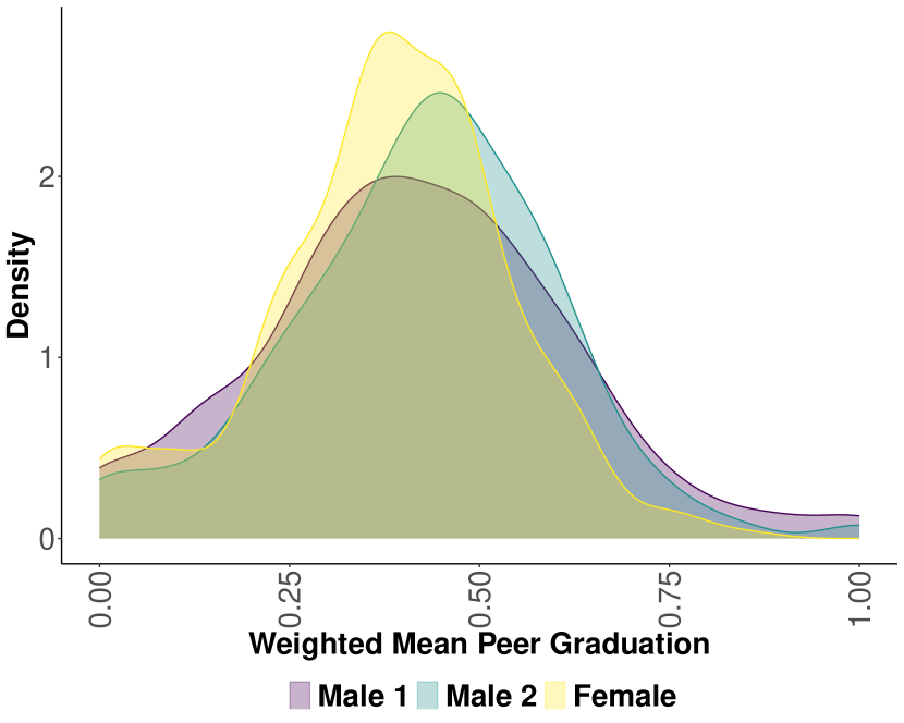
a. Graduation Status of peers

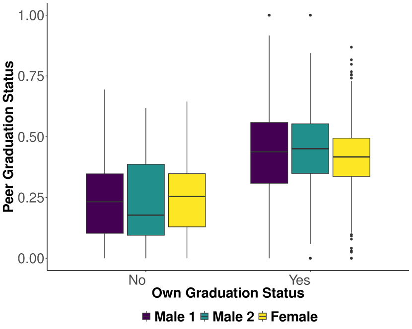
b. Peer graduation and success

Notes: We pool the data across three units for these figures. The final data-sets includes the residents for whom we observe the complete set of covariates and the affirmations network. Panel (a) shows the distribution of peer graduation status weighed by the nodes of the affirmation network as observed by residents at time $t$ when survey for graduation status was conducted. Panel (b) displays the correlation between the peer graduation as observed by each resident and their own graduation status.

Figure B2: Out of Sample AUC for Selection of $d$ using Cross-validation

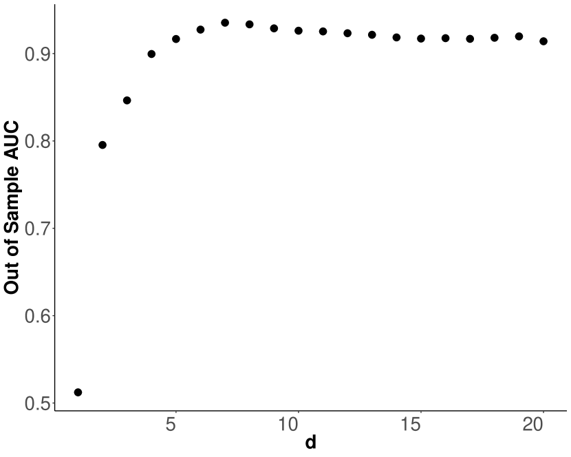
a. Male Unit 1

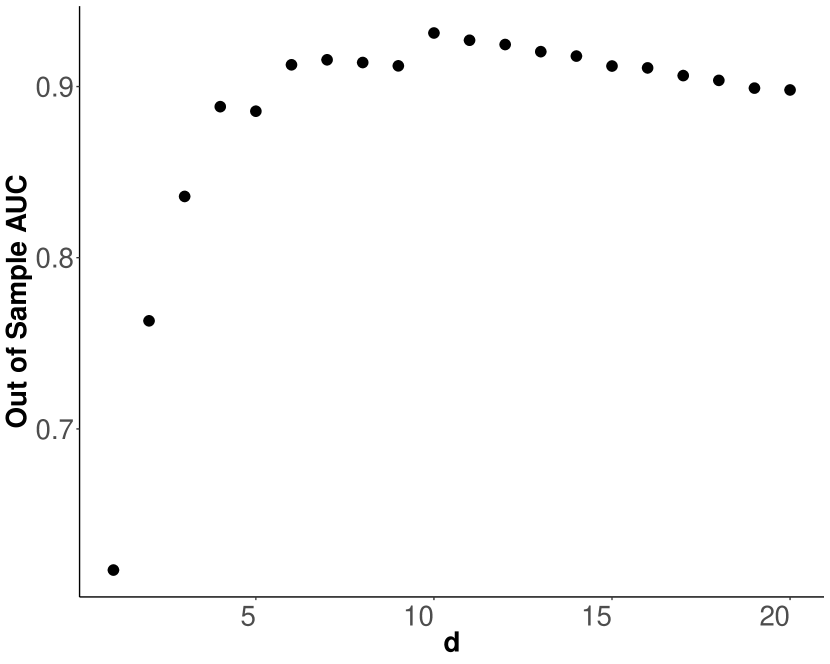
b. Male Unit 2

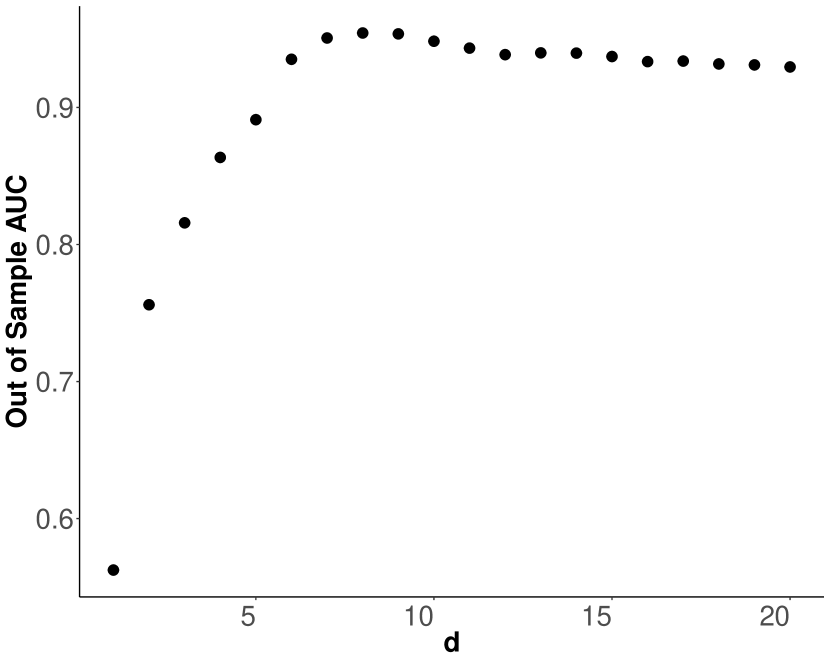
c. Female Unit

Notes: Figures (a,b and c) illustrate the out of sample as we increase $d$ from 1 to 20 in male unit 1, male unit 2 and female unit respectively. The $d$ for each unit is chosen via cross-validation using the out-of-sample AUCs.

Figure B3: Misclassification Error

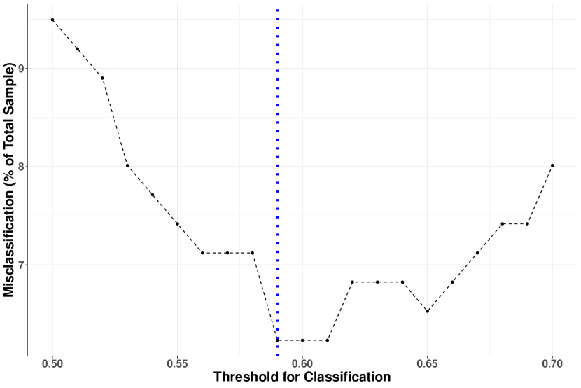
a. Male Unit 1

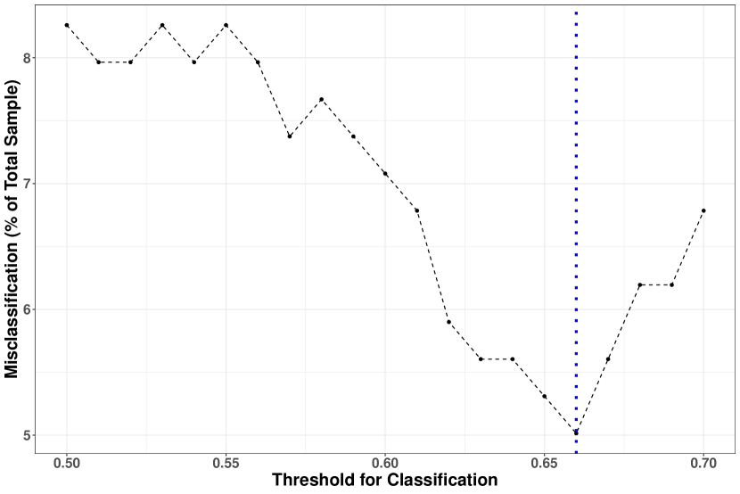
b. Male Unit 2

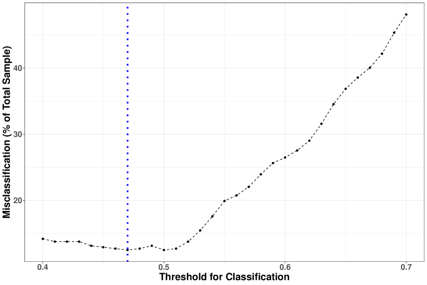
c. Female Unit

Notes: Figures (a,b and c) illustrate the misclassification error as the threshold changes. We choose the threshold that corresponds to the case with lowest misclassification error.

References

- Andrews and Bonta, (1995) Andrews, D. and Bonta, J. (1995). The level of service inventory-revised [user manual]. toronto, on: Multi-health systems.
- Aral and Nicolaides, (2017) Aral, S. and Nicolaides, C. (2017). Exercise contagion in a global social network. Nature communications, 8:14753.
- Athreya et al., (2017) Athreya, A., Fishkind, D. E., Tang, M., Priebe, C. E., Park, Y., Vogelstein, J. T., Levin, K., Lyzinski, V., and Qin, Y. (2017). Statistical inference on random dot product graphs: a survey. The Journal of Machine Learning Research, 18(1):8393–8484.
- Athreya et al., (2016) Athreya, A., Priebe, C. E., Tang, M., Lyzinski, V., Marchette, D. J., and Sussman, D. L. (2016). A limit theorem for scaled eigenvectors of random dot product graphs. Sankhya A, 78(1):1–18.
- Baird et al., (2023) Baird, M. D., Engberg, J., and Opper, I. M. (2023). Optimal allocation of seats in the presence of peer effects: Evidence from a job training program. Journal of Labor Economics, 41(2):479–509.
- BB and Mutton, (1975) BB, D. and Mutton, B. (1975). The effect of errors in the independent variables in linear regression. Biometrika, 62(2):383–391.
- Best, (2019) Best, D. (2019). What we know about recovery, desistance and reintegration. In Pathways to Recovery and Desistance, pages 1–22. Policy Press.
- Bramoullé et al., (2009) Bramoullé, Y., Djebbari, H., and Fortin, B. (2009). Identification of peer effects through social networks. Journal of econometrics, 150(1):41–55.
- Cacioppo et al., (2009) Cacioppo, J. T., Fowler, J. H., and Christakis, N. A. (2009). Alone in the crowd: the structure and spread of loneliness in a large social network. Journal of personality and social psychology, 97(6):977.
- Campbell et al., (2021) Campbell, B., Warren, K., Weiler, M., and De Leon, G. (2021). Eigenvector centrality defines hierarchy and predicts graduation in therapeutic community units. Plos one, 16(12):e0261405.
- Chan et al., (2014) Chan, T. Y., Li, J., and Pierce, L. (2014). Compensation and peer effects in competing sales teams. Management Science, 60(8):1965–1984.
- Chang et al., (2012) Chang, Y.-P., Lin, Y.-C., and Chen, L. H. (2012). Pay it forward: Gratitude in social networks. Journal of Happiness Studies, 13:761–781.
- Christakis and Fowler, (2007) Christakis, N. A. and Fowler, J. H. (2007). The spread of obesity in a large social network over 32 years. New England journal of medicine, 357(4):370–379.
- Christakis and Fowler, (2008) Christakis, N. A. and Fowler, J. H. (2008). The collective dynamics of smoking in a large social network. New England journal of medicine, 358(21):2249–2258.
- Coviello et al., (2014) Coviello, L., Sohn, Y., Kramer, A. D., Marlow, C., Franceschetti, M., Christakis, N. A., and Fowler, J. H. (2014). Detecting emotional contagion in massive social networks. PloS one, 9(3):e90315.
- De Leon et al., (1982) De Leon, G., Wexler, H. K., and Jainchill, N. (1982). The therapeutic community: Success and improvement rates 5 years after treatment. International Journal of the Addictions, 17(4):703–747.
- Dean et al., (2017) Dean, D. O., Bauer, D. J., and Prinstein, M. J. (2017). Friendship dissolution within social networks modeled through multilevel event history analysis. Multivariate behavioral research, 52(3):271–289.
- Fowler and Christakis, (2008) Fowler, J. H. and Christakis, N. A. (2008). Dynamic spread of happiness in a large social network: longitudinal analysis over 20 years in the framingham heart study. Bmj, 337:a2338.
- Goldsmith-Pinkham and Imbens, (2013) Goldsmith-Pinkham, P. and Imbens, G. W. (2013). Social networks and the identification of peer effects. Journal of Business Economic Statistics, 31(3):253–264.
- Gossop, (2000) Gossop, M. (2000). The therapeutic community: Theory, model and method. Addiction, 95(11):1720.
- Handcock et al., (2007) Handcock, M. S., Raftery, A. E., and Tantrum, J. M. (2007). Model-based clustering for social networks. Journal of the Royal Statistical Society: Series A (Statistics in Society), 170(2):301–354.
- Herbst and Mas, (2015) Herbst, D. and Mas, A. (2015). Peer effects on worker output in the laboratory generalize to the field. Science, 350(6260):545–549.
- Hernán and Cole, (2009) Hernán, M. A. and Cole, S. R. (2009). Invited commentary: causal diagrams and measurement bias. American journal of epidemiology, 170(8):959–962.
- Hoff et al., (2002) Hoff, P. D., Raftery, A. E., and Handcock, M. S. (2002). Latent space approaches to social network analysis. Journal of the american Statistical association, 97(460):1090–1098.
- Holland et al., (1983) Holland, P., Laskey, K., and Leinhardt, S. (1983). Stochastic blockmodels: some first steps. Social Networks, 5:109–137.
- Hsieh and Lee, (2016) Hsieh, C.-S. and Lee, L. F. (2016). A social interactions model with endogenous friendship formation and selectivity. Journal of Applied Econometrics, 31(2):301–319.
- Jason et al., (2022) Jason, L. A., Lynch, G., Bobak, T., Light, J. M., and Doogan, N. J. (2022). Dynamic interdependence of advice seeking, loaning, and recovery characteristics in recovery homes. Journal of Human Behavior in the Social Environment, 32(5):663–678.
- Kramer et al., (2014) Kramer, A. D., Guillory, J. E., and Hancock, J. T. (2014). Experimental evidence of massive-scale emotional contagion through social networks. Proceedings of the National Academy of Sciences, 111(24):8788–8790.
- Kreager et al., (2019) Kreager, D. A., Schaefer, D. R., Davidson, K. M., Zajac, G., Haynie, D. L., and De Leon, G. (2019). Evaluating peer-influence processes in a prison-based therapeutic community: a dynamic network approach. Drug and alcohol dependence, 203:13–18.
- Lazer, (2001) Lazer, D. (2001). The co-evolution of individual and network. Journal of Mathematical Sociology, 25(1):69–108.
- Lazer et al., (2010) Lazer, D., Rubineau, B., Chetkovich, C., Katz, N., and Neblo, M. (2010). The coevolution of networks and political attitudes. Political Communication, 27(3):248–274.
- Leenders, (2002) Leenders, R. T. A. (2002). Modeling social influence through network autocorrelation: constructing the weight matrix. Social networks, 24(1):21–47.
- Lei and Rinaldo, (2015) Lei, J. and Rinaldo, A. (2015). Consistency of spectral clustering in stochastic block models. The Annals of Statistics, 43(1):215–237.
- Manski, (1993) Manski, C. F. (1993). Identification of endogenous social effects: The reflection problem. The review of economic studies, 60(3):531–542.
- Marsden and Friedkin, (1993) Marsden, P. V. and Friedkin, N. E. (1993). Network studies of social influence. Sociological Methods & Research, 22(1):127–151.
- McFowland III and Shalizi, (2021) McFowland III, E. and Shalizi, C. R. (2021). Estimating causal peer influence in homophilous social networks by inferring latent locations. Journal of the American Statistical Association, pages 1–12.
- McPherson et al., (2001) McPherson, M., Smith-Lovin, L., and Cook, J. M. (2001). Birds of a feather: Homophily in social networks. Annual review of sociology, 27(1):415–444.
- Mericle et al., (2023) Mericle, A. A., Howell, J., Borkman, T., Subbaraman, M. S., Sanders, B. F., and Polcin, D. L. (2023). Social model recovery and recovery housing. Addiction Research & Theory, pages 1–8.
- Nakamura, (1990) Nakamura, T. (1990). Corrected score function for errors-in-variables models: Methodology and application to generalized linear models. Biometrika, 77(1):127–137.
- Novick and Stefanski, (2002) Novick, S. J. and Stefanski, L. A. (2002). Corrected score estimation via complex variable simulation extrapolation. Journal of the American Statistical Association, 97(458):472–481.
- Paul and Chen, (2016) Paul, S. and Chen, Y. (2016). Consistent community detection in multi-relational data through restricted multi-layer stochastic blockmodel. Electronic Journal of Statistics, 10(2):3807–3870.
- Paul et al., (2020) Paul, S., Chen, Y., et al. (2020). A random effects stochastic block model for joint community detection in multiple networks with applications to neuroimaging. Annals of Applied Statistics, 14(2):993–1029.
- Pearl, (2009) Pearl, J. (2009). Causality. Cambridge university press.
- Riessman, (1965) Riessman, F. (1965). The” helper” therapy principle. Social work, pages 27–32.
- Rohe et al., (2011) Rohe, K., Chatterjee, S., and Yu, B. (2011). Spectral clustering and the high-dimensional stochastic blockmodel. Ann. Statist, 39(4):1878–1915.
- Roxburgh et al., (2023) Roxburgh, A. D., Best, D., Lubman, D. I., and Manning, V. (2023). Composition of social networks to build recovery capital differ across early and stable stages of recovery. Addiction Research & Theory, pages 1–8.
- Rubin-Delanchy et al., (2022) Rubin-Delanchy, P., Cape, J., Tang, M., and Priebe, C. E. (2022). A statistical interpretation of spectral embedding: The generalised random dot product graph. Journal of the Royal Statistical Society Series B: Statistical Methodology, 84(4):1446–1473.
- Sacerdote, (2011) Sacerdote, B. (2011). Peer effects in education: How might they work, how big are they and how much do we know thus far? In Handbook of the Economics of Education, volume 3, pages 249–277. Elsevier.
- Schafer, (1987) Schafer, D. W. (1987). Covariate measurement error in generalized linear models. Biometrika, 74(2):385–391.
- Shalizi and Thomas, (2011) Shalizi, C. R. and Thomas, A. C. (2011). Homophily and contagion are generically confounded in observational social network studies. Sociological methods & research, 40(2):211–239.
- Snijders, (2017) Snijders, T. A. (2017). Stochastic actor-oriented models for network dynamics. Annual review of statistics and its application, 4:343–363.
- Sridhar et al., (2022) Sridhar, D., De Bacco, C., and Blei, D. (2022). Estimating social influence from observational data. In Conference on Causal Learning and Reasoning, pages 712–733. PMLR.
- Stefanski, (1985) Stefanski, L. A. (1985). The effects of measurement error on parameter estimation. Biometrika, 72(3):583–592.
- Stefanski et al., (1985) Stefanski, L. A., Carroll, R. J., et al. (1985). Covariate measurement error in logistic regression. The Annals of Statistics, 13(4):1335–1351.
- Sussman et al., (2012) Sussman, D. L., Tang, M., Fishkind, D. E., and Priebe, C. E. (2012). A consistent adjacency spectral embedding for stochastic blockmodel graphs. Journal of the American Statistical Association, 107(499):1119–1128.
- Tang et al., (2018) Tang, M., Priebe, C. E., et al. (2018). Limit theorems for eigenvectors of the normalized laplacian for random graphs. The Annals of Statistics, 46(5):2360–2415.
- VanderWeele, (2011) VanderWeele, T. J. (2011). Sensitivity analysis for contagion effects in social networks. Sociological Methods & Research, 40(2):240–255.
- VanderWeele and An, (2013) VanderWeele, T. J. and An, W. (2013). Social networks and causal inference. In Handbook of causal analysis for social research, pages 353–374. Springer.
- (59) Warren, K., Campbell, B., and Cranmer, S. (2020a). Tightly bound: the relationship of network clustering coefficients and reincarceration at three therapeutic communities. Journal of Studies on Alcohol and Drugs, 81(5):673–680.
- (60) Warren, K., Campbell, B., Cranmer, S., De Leon, G., Doogan, N., Weiler, M., and Doherty, F. (2020b). Building the community: Endogenous network formation, homophily and prosocial sorting among therapeutic community residents. Drug and Alcohol Dependence, 207:107773.
- (61) Warren, K., Doogan, N. J., and Doherty, F. (2021a). Difference in response to feedback and gender in three therapeutic community units. Frontiers in Psychiatry, 12.
- Warren, (2020) Warren, K. L. (2020). Senior therapeutic community members show greater consistency when affirming peers: evidence of social learning. Therapeutic Communities: The International Journal of Therapeutic Communities.
- (63) Warren, K. L., Doogan, N., Wernekinck, U., and Doherty, F. C. (2021b). Resident interactions when affirming and correcting peers in a therapeutic community for women. Therapeutic Communities: The International Journal of Therapeutic Communities.
- White and Kurtz, (2008) White, W. L. and Kurtz, E. (2008). Twelve defining moments in the history of alcoholics anonymous. Recent Developments in Alcoholism: Research on Alcoholics Anonymous and Spirituality in Addiction Recovery, pages 37–57.
- Yates et al., (2017) Yates, R., Burns, J., and McCabe, L. (2017). Integration: Too much of a bad thing? Journal of Groups in Addiction & Recovery, 12(2-3):196–206.