+91 86306 46746; +91 9632928096 Indian Institute of Science] Department of Inorganic and Physical Chemistry, Indian Institute of Science, Bangalore 560012, India IR,NMR,UV IR,NMR,UV

A demonstration of the achemso LaTeX class

Exact Results for the Tavis-Cummings and H$\boldsymbol{\ddot{u}}$ckel Hamiltonians with Diagonal Disorder

Abstract

We present an exact method to calculate the electronic states of one electron Hamiltonians with diagonal disorder. We show that the disorder averaged one particle Green’s function can be calculated directly, using a deterministic complex (non-Hermitian) Hamiltonian. For this, we assume that the molecular states have a Cauchy (Lorentz) distribution and use the supersymmetric method which has already been used in problems of solid state physics. Using the method we find exact solutions to the states of $N$ molecules, confined to a microcavity, for any value of $N$. Our analysis shows that the width of the polaritonic states as a function of $N$ depend on the nature of disorder, and hence can be used to probe the way molecular energy levels are distributed. We also show how one can find exact results for H$\ddot{u}$ckel type Hamiltonians with on-site, Cauchy disorder and demonstrate its use.

Confining molecules to micro-cavities of size such that a molecular excitation (electronic or vibrational) is resonant with an electromagnetic mode of the cavity leads to the formation of hybrid light-matter states known as polaritons. Such confinement can cause modifications of the rates of chemical processes. Rather than giving an extensive list of the many interesting developments in the area, we refer the reader to the summaries that may be found in Ebbesen et. al¹, Hartland and Scholes² and Herrera and Owrutsky³.

Light-matter coupling leads to the formation a lower and an upper polaritonic states and the energy difference between the two is the Rabi splitting $\Omega.$ The polaritonic states are an example of collective phenomena where states of a large number $N$ of molecules combine to form one state, which then combines with the cavity mode to give the two polaritonic states. The value of $N$ is very large - roughly speaking, all the molecules which are oriented in the direction of the electric field of the cavity, located at points where the electric field of the cavity mode is not very small couple. It is the coupling of this large number of molecules that leads to the large Rabi splitting whose frequency is a sizeable fraction of the energy of the molecular excitation involved. The formation of the polaritonic states is usually understood using the Tavis-Cummings ⁴ model which has $N$ excitations localized on each molecule, all having the energy $\epsilon_{a}$ and the cavity mode of energy $\epsilon_{c}$. In this simple model the $N-1$ modes that remain are completely decoupled from the radiation and hence are referred to as the dark states. While this is the ideal situation, there would be disorder in the molecular energy levels due to various reasons ⁵. The causes for this may be inhomogeneities in the material, different levels of aggregation of the molecules, solvent fluctuations or dispersal by solvent. Hence a generalized version of the Tavis-Cummings Hamiltonian with disorder has been the subject of a few recent papers ^{6, 7, 8, 9, 10} which give approximate ways of analyzing the problem.

Scholes ⁵ in an interesting paper studied excitation energy transfer in a finite collection of molecules arranged in different topologies, varying from linear to the star. A H$\ddot{u}$ckel type Hamiltonian with nearest neighbor hopping was used as the model. The effect of diagonal disorder on the spectrum of the eigenvalues as well as the inverse participation ratio was investigated. The diagonal disorder on the sites were taken to be independent identically distributed Gaussian random variables and all the quantities were numerically calculated. Among all topologies considered, the star graph (star topology) was found to have the most stable eigenvalue spectrum. Very interestingly, the Tavis-Cummings Hamiltonian has the same topology as the star graph.

In this paper we point out that it is possible to find exact results for an arbitrary one electron Hamiltonian with diagonal disorder, provided the disorder has a Cauchy distribution. The disorder numerically studied by Scholes is one in which the energy of a given site $``i"$ is given by $\epsilon_{a}+\xi_{i}$ with $\xi_{i}$ following the Gaussian distribution. In comparison, the Cauchy or Lorentz distribution is given by $P(\xi_{i})=\frac{\gamma}{\pi(\gamma^{2}+\xi_{i}^{2})}$. It has been realized long ago by Lloyd ¹¹ that some exact results can be calculated analytically for tight binding model Hamiltonians with site disorder having a Cauchy distribution. An elegant method to show this is the use of Grassmann variables ^{12, 13}. We give the barest minimum details of the method.

We consider a one electron Hamiltonian which may be written as $\hat{H}=\sum_{i,j}^{N}H_{ij}|i\rangle\langle j|,$ with diagonal disorder. $N$ is the number of sites, each having an orbital $\left|i\right\rangle$. $H_{ij}$ represents the hopping matrix element between the $i^{th}$ and $j^{th}$ sites. The site energy $H_{ii}$ has disorder and is given by $H_{ii}=\epsilon_{a}+\xi_{i},$ where $\xi_{i}$ is the random component, having the Cauchy probability distribution $P(\xi_{i})$. We shall use the symbol $\boldsymbol{H}$ to denote the matrix with matrix elements $H_{ij}$. We denote by $<..>_{\boldsymbol{\xi}}$ the average over all $\xi_{i}$s and clearly, the mean value $<\xi_{i}>_{\boldsymbol{\xi}}=0$. We are interested in calculating the Green’s matrix $\boldsymbol{G}(\omega)=\left(\omega-\boldsymbol{H}\right)^{-1}$ and its average $<\boldsymbol{G}(\omega)>_{\boldsymbol{\xi}}$. The matrix elements of $\boldsymbol{G}(\omega)$ are very useful for the calculation of the one-particle properties of the system. For example, defining the eigenstates $|m\rangle$ of the Hamiltonian by $\hat{H}|m\rangle=\varepsilon_{m}|m\rangle$ we can calculate $\rho_{i}(\omega)$ the one particle density of states on the $i^{th}$ orbital $|i\rangle$. $\rho_{i}(\omega)=\sum_{m}\left|\left\langle i\left|m\right.\right\rangle\right|^{2}\delta(\omega-\varepsilon_{m})=-\frac{1}{\pi}Im\left[G_{ii}(\omega+i\eta)\right]$, with $\eta$ being positive and infinitesimal. The quantity that is of greatest interest is the average of the density of states on the $i^{th}$ site $\left\langle\rho_{i}(\omega)\right\rangle_{\boldsymbol{\xi}},$ which implies that we need to calculate $\left\langle G_{ii}(\omega+i\eta)\right\rangle_{\boldsymbol{\xi}}$. For this we follow Zinn-Justin ¹³ and define a “generating function", $\mathfrak{Z}(\boldsymbol{A},\boldsymbol{b},\overline{\boldsymbol{b}})=\int\left(\prod_{i=1}^{N}\frac{dz_{i}d\overline{z}_{i}}{2\pi i}\right)\exp\left(-\overline{\boldsymbol{z}}.\boldsymbol{A}.\boldsymbol{z}+\overline{\boldsymbol{b}}.\boldsymbol{z}+\overline{\boldsymbol{z}}.\boldsymbol{b}\right),$where $\boldsymbol{z}=(z_{1,}z_{2},z_{3},...z_{N})^{T}$, $z_{i}$ being a complex variable and the $\boldsymbol{\overline{z}}=(\overline{z}_{1},\overline{z}_{2},...\overline{z}_{N}),$ where “bar" is used to denote the complex conjugate. $\boldsymbol{b}=(b_{1,}b_{2},b_{3},..b_{N})^{T}$ and $\boldsymbol{\overline{b}}=(\overline{b}_{1},\overline{b}_{2},..\overline{b}_{N})$ with $b_{i}$ arbitrary complex variables. The superscript $T$ is used to denote transpose of a matrix and $\overline{\boldsymbol{z}}.\boldsymbol{A}.\boldsymbol{z}=\sum_{i,j=1}^{N}\bar{z}_{i}A_{ij}z_{j},$ where $\boldsymbol{A}$ is the matrix having $A_{ij}$ as its matrix elements. Zinn-Justin ¹³ shows that $\mathfrak{Z}(\boldsymbol{A},\boldsymbol{b},\overline{\boldsymbol{b}})=|\boldsymbol{A}|^{-1}\exp\left(\overline{\boldsymbol{b}}.\boldsymbol{A^{-1}}.\boldsymbol{b}\right),$ and gives the conditions under which this is true. Here $|\boldsymbol{A}|$ stands for the determinant of the matrix $\boldsymbol{A}$. This can be rearranged to get $\left[\frac{\partial^{2}}{\partial\overline{b}_{i}\partial b_{j}}\mathfrak{Z}(\boldsymbol{A},\boldsymbol{b},\overline{\boldsymbol{b}})\right]_{\boldsymbol{b}=\boldsymbol{0}}=|\boldsymbol{A}|^{-1}\left(\boldsymbol{A}^{-1}\right)_{ij},$

$$\left(\boldsymbol{A}^{-1}\right)_{ij}=\left[|\boldsymbol{A}|\frac{\partial^{2}}{\partial\overline{b}_{i}\partial b_{j}}\mathfrak{Z}(\boldsymbol{A},\boldsymbol{b},\overline{\boldsymbol{b}})\right]_{\boldsymbol{b}=\boldsymbol{0}}.$$ (1)

For calculating $G_{ij}(\omega+i\eta)$ we put $\boldsymbol{A}=$$-i(\omega+i\eta-\boldsymbol{H)}$ . The quantity $\eta$ ensures that the integral in the definition of $\mathfrak{Z}(\boldsymbol{A},\boldsymbol{b},\overline{\boldsymbol{b}})$ is convergent. From Eq. (1), we find

$$\left\langle\left[(\omega+i\eta-\boldsymbol{H)}^{-1}\right]_{ii}\right\rangle_{\boldsymbol{\xi}}=\left[\frac{\partial^{2}}{\partial\overline{b}_{i}\partial b_{j}}\left\langle\det|-i(\omega+i\eta-\boldsymbol{H)}|\mathfrak{\quad Z}({-i(\omega+i\eta-\boldsymbol{H)}},\boldsymbol{b},\overline{\boldsymbol{b}})\right\rangle_{\boldsymbol{\xi}}\right]_{\boldsymbol{b}=\boldsymbol{0}}.$$ (2)

In our case $\boldsymbol{H}$ has the random component $\boldsymbol{\xi}$ which needs to be averaged over $\boldsymbol{\xi}$ as indicated on the right hand side of the above equation. This averaging seems impossible, because it is a product of the determinant and the quantity $\mathfrak{\quad Z}({-i(\omega+i\eta-\boldsymbol{H)}},\boldsymbol{b},\overline{\boldsymbol{b}})$ both of them dependent on $\boldsymbol{\xi}.$ Interestingly, it is possible to write the determinant in a form such that the averaging can be done easily using Grassmann variables ^{13, 12}. We note that $|-i(\omega+i\eta-\boldsymbol{H)}|=\int d\overline{\boldsymbol{\rho}}d\boldsymbol{\rho}e^{i\overline{\boldsymbol{\rho}}(\omega+i\eta-\boldsymbol{H)\boldsymbol{\rho}}},$ where $\boldsymbol{\rho}=\left(\rho_{1},\rho_{2},...\rho_{N}\right)^{T}$ and $\overline{\boldsymbol{\rho}}=\left(\overline{\rho}_{1},\overline{\rho}_{2},...\overline{\rho}_{N}\right)$ are both collections of $N$ Grassmann variables, $\bar{\rho_{i}}$ being the complex conjugate of $\rho_{i}.$ Hence,

$$\left\langle\left[(\omega+i\eta-\boldsymbol{H)}^{-1}\right]_{ii}\right\rangle_{\boldsymbol{\xi}}=\left[\frac{\partial^{2}}{\partial b_{i}^{*}\partial b_{j}}\int d\boldsymbol{z}d\overline{\boldsymbol{z}}\int d\overline{\boldsymbol{\rho}}d\boldsymbol{\rho}\left\langle e^{i\overline{\boldsymbol{\rho}}(\omega+i\eta-\boldsymbol{H})\boldsymbol{\rho}+i\overline{\boldsymbol{z}}(\omega+i\eta-\boldsymbol{H})\boldsymbol{z}+\overline{\boldsymbol{b}}.\boldsymbol{z}+\overline{\boldsymbol{z}}.\boldsymbol{b}}\right\rangle_{\boldsymbol{\xi}}\right]_{\boldsymbol{b}=\boldsymbol{0}}.$$ (3)

The integral in the above is over ordinary variables as well as the anti-commuting Grassmann variables and is referred to as a superintegral and the approach itself as the supersymmetric method. As the $\xi_{j}$s in Eq. (3) appears in the exponential, one can average each $\xi_{j}$ separately. The result of collecting together just the terms that depend on $\xi_{j}$ and then averaging is demonstrated below:

$$\left\langle e^{-i\xi_{j}(\rho_{j}^{*}\rho_{j}+z_{j}^{*}z_{j})}\right\rangle_{\boldsymbol{\xi}} = \frac{\gamma}{\pi}\int_{-\infty}^{\infty}d\xi_{j}\frac{\exp\left\{i\xi_{j}(\rho_{j}^{*}\rho_{j}+z_{j}^{*}z_{j})\right\}}{(\gamma^{2}+\xi_{j}^{2})}=e^{-\gamma(\rho_{j}^{*}\rho_{j}+z_{j}^{*}z_{j})}.$$ (4)

Using Eq. (4) in Eq. (3) we get

$\left\langle\left[{(\omega+i\eta-\boldsymbol{H})}^{-1}\right]_{ii}\right\rangle_{\boldsymbol{\xi}}=\left[\frac{\partial^{2}}{\partial b_{i}^{*}\partial b_{j}}\int d\boldsymbol{z}d\overline{\boldsymbol{z}}\int d\overline{\boldsymbol{\rho}}d\boldsymbol{\rho}e^{i\overline{\boldsymbol{\rho}}(\omega-\boldsymbol{H}_{0}+i\gamma\boldsymbol{I})\boldsymbol{\rho}+i\overline{\boldsymbol{z}}(\omega-\boldsymbol{H}_{0}+i\gamma\boldsymbol{I})\boldsymbol{z}+\overline{\boldsymbol{b}}.\boldsymbol{z}+\overline{\boldsymbol{z}}.\boldsymbol{b}}\right]_{\boldsymbol{b}=\boldsymbol{0}},\\$ which simplifies the calculation enormously. It shows that for the purpose of the calculation of the averaged quantity, the random Hamiltonian can be replaced with a complex one in which the random term $\xi_{i}$ is simply replaced by the non-random imaginary quantity $-i\gamma$. Thus one has the complex, non-Hermitian Hamiltonian $\hat{\cal H}=\sum_{i}^{N}(\epsilon_{a}-i\gamma)|i\rangle\langle i|+\sum_{i\neq j}^{N}\left\{H_{ij}|i\rangle\langle i|+H_{ji}|i\rangle\langle i|\right\},$ for which we need to calculate the Green’s matrix. From this the averaged density of states on the $i^{th}$ site may be easily calculated as $\langle\rho_{ii}(\omega)\rangle_{\boldsymbol{\xi}}=-\frac{1}{\pi}Im\langle i|\left(\omega-\hat{\cal H}\right)^{-1}|i\rangle.$ We now proceed to illustrate the utility of the approach for two Hamiltonians with diagonal disorder. They are the Tavis-Cummings Hamiltonian for molecules confined to a microcavity and the H$\ddot{u}$ckel type Hamiltonian for describing exciton transfer.

A problem of great current interest is the different excited states of a large number of molecules put inside a cavity of size such that a molecular excitation is nearly resonant with a standing mode of the cavity. This is modelled by the Tavis-Cummings Hamiltonian for which exact solution is easy to find. However, there are only approximate analyses for the case where the molecular excitation energies are randomly distributed around a mean. Recently, we have obtained an approximate analytic solution for the case the excitation energies have a Gaussian distribution ¹⁰. The solution is expected to asymptotically approach the exact solution as the number of molecules $N\rightarrow\infty.$ Using the method outlined above, we can find the analytic solution any value of $N$, small or large. In our model, the excitation energy $\epsilon_{i}$ of the $i^{th}$ molecule is taken as $\epsilon_{i}=\epsilon_{a}+\xi_{i},$ where $\xi_{i}$s are identically distributed random variables having the Cauchy probability distribution.

With such a disorder, the Hamiltonian may be written as $\hat{H}=\epsilon_{c}|c\rangle\langle c|+\sum_{i}^{N}(\epsilon_{a}+\xi_{i})|i\rangle\langle i|+\sum_{i}^{N}(V_{i}|c\rangle\langle i|+V_{i}^{*}|i\rangle\langle c|).$ $|c\rangle$ denotes the state where the cavity mode is excited to its first excited level. It has an energy of $\epsilon_{c}$. $|i\rangle$ denotes the state in which the $i^{th}$ molecule is excited. This problem has $N+1$ states, one from the cavity and one each from the $N$ molecules. The coupling constant of the cavity mode to the excited state of the $i^{th}$ molecule is denoted by $V_{i}$ and is given by $V_{i}=-\boldsymbol{E}(z_{i}).\boldsymbol{{\mu}}_{i}=-\mu_{eg}\sqrt{\frac{\epsilon_{c}}{2\epsilon_{o}{\cal V}}}=V,$ where we have assumed that all the molecules are oriented in the direction of the electric field $\boldsymbol{E}(z_{i})$ of the cavity and that the positional variation of the electric field may be neglected. ${\cal V}$ is the volume of the cavity and $\boldsymbol{{\mu}}_{i}$ is transition dipole moment of the molecular excitation, having the magnitude $\mu_{eg}$. The permittivity of matter and that of free space are denoted as $\epsilon_{c}$ and $\epsilon_{o}$ respectively. In the following, letters like $G,\boldsymbol{G},\hat{H},...$ are quantities that depend on the disorder $\boldsymbol{\xi}$. Symbols like $\cal{G},\boldsymbol{{\cal G}},\boldsymbol{{\cal H}},.....$ are quantities that have been averaged over $\boldsymbol{\xi}$.

To calculate $\left\langle G_{ij}(\omega)\right\rangle_{\boldsymbol{\xi}}=\langle i|\left[\omega-\hat{\cal H}\right]^{-1}|j\rangle,$ we need to use the complex Hamiltonian with all the random terms replaced with $-i\gamma$. This gives the new Hamiltonian $\hat{\cal H}=\epsilon_{c}|c\rangle\langle c|+\sum_{i}^{N}(\epsilon_{a}-i\gamma)|i\rangle\langle i|+\sum_{i}^{N}(V_{i}|c\rangle\langle i|+V_{i}|i\rangle\langle c|).$ We now proceed to determine the matrix elements of $\hat{\cal G}(\omega)=(\omega-\hat{\cal H})^{-1}$ following ¹⁰ and find ${\cal G}_{cc}(\omega)=\left[\omega-\epsilon_{c}-{\Sigma}(\omega)\right]^{-1},$ with the self energy $\Sigma(\omega)=\sum_{i=1}^{N}\frac{V_{i}^{2}}{\omega-\epsilon_{a}+i\gamma}=\frac{NV^{2}}{\omega-\epsilon_{a}+i\gamma}=\frac{{\cal N}\tilde{V}^{2}}{\omega-\epsilon_{a}+i\gamma}.$ We have defined $\tilde{V}=\sqrt{\cal{V}}V$ and the number density of molecules within the cavity ${\cal N}=N/\cal{V}$. See the Supporting Information for more details. Then ${\cal G}_{cc}(\omega)=\left[\omega-\epsilon_{c}-\frac{{\cal N}\tilde{V}^{2}}{\omega-\epsilon_{a}+i\gamma}\right]^{-1}.$ The poles of ${\cal G}_{cc}(\omega)$ are at $\epsilon_{\pm}=\frac{\left(\epsilon_{a}+\epsilon_{c}-i\gamma\right)}{2}\pm\sqrt{{\cal N}\tilde{V}^{2}+\left(\frac{\epsilon_{c}-\epsilon_{a}-i\gamma}{2}\right)^{2}}.$ The real part of $\epsilon_{\pm}$ determine the energies of the two polaritonic states and the imaginary part its lifetime.

The widths of the peaks are determined by the imaginary part of $\epsilon_{\pm}$. In the limit of large $\sqrt{\cal{N}}|\tilde{V}|$ it is found to be $-i\gamma/2$. This means that the two polaritons have the same width, which is equal to half the width of the distribution of the molecular states. We note that the widths of the polaritonic peaks are very sensitive to the nature of the distribution of molecular energy levels, i.e., the probability distribution $P(\xi_{i})$. In our previous work ¹⁰ we had analyzed the case of Gaussian distribution and found that the width decreases as the value of $\cal N$ becomes large. In the case of Cauchy distribution, the width remains constant provided $\sqrt{\cal{N}}|\tilde{V}|\gg\gamma$. On the other hand, if $P(\xi_{i})$ is taken as a uniform distribution in the range $(-w,w),$ then it is found that the polarionic peaks are Dirac delta functions. The absorption cross-section is given by ¹⁰: $\alpha(\omega)=-\frac{\omega}{\epsilon_{o}c\hbar}N\left|\boldsymbol{{\mu}}\right|^{2}\;Im\left[{\cal G}_{mol,mol}(\omega)\right]$ where, ${\cal G}_{mol,mol}(\omega)=(\omega-\epsilon_{c}){\cal{G}}_{cc}(\omega)\frac{1}{\mathscr{N}\tilde{V}^{2}}\Sigma(\omega).$ Derivations for this as well as other quantities may be found in the Supporting Information.

In Fig. 1 the cavity density of states is plotted against $\omega$ with varying values of $\gamma$. The cavity state is divided amongst the two polaritonic states with total area under the two peaks equals to unity. As the value of $\gamma$ increases the peak width increases as we would expect.

Figure 1: Plot for $<\rho_{c}(\omega)>_{\boldsymbol{\xi}}$ against $\omega$ for $\mathscr{N}=1.16\times 10^{25}m^{-3}$ and different values of $\gamma$. Following values were used $\epsilon_{c}=2.1\,eV$, $\epsilon_{a}=\epsilon_{c}$, $\tilde{V}=4.06\times 10^{-14}\,eVm^{3/2}$.

In Fig. 2 the change in molecular density of states $\Delta\rho_{M}(\omega)$ (expression given in Supporting Information), $\omega$ with varying values of $\gamma$. Integrating the area under the curve from $\omega=2.0\;eV$ to $\omega=2.2\;eV$ results in the value of $-1$. This means that out of the $N$ states, effectively one state contributes to the polariton formation. Further, the dip in the middle means that the states which are in close resonance to the cavity state contributes the largest to the polaritons.

Figure 2: Plot for $<\Delta\rho_{M}(\omega)>_{\boldsymbol{\xi}}$ against $\omega$ for $\mathscr{N}=1.16\times 10^{25}m^{-3}$ and different values of $\gamma$. Following values were used $\epsilon_{c}=2.1\,eV$, $\epsilon_{a}=\epsilon_{c}$, $\tilde{V}=4.06\times 10^{-14}\,eVm^{3/2}$.

It is possible to calculate absorption spectrum of the system using expressions given in Supporting Information, for varied values of $\gamma$ and the results are shown in Fig. 3.

Figure 3: Plot for absorption cross section $<\alpha(\omega)>_{\boldsymbol{\xi}}$ against $\omega$ for $\mathscr{N}=1.16\times 10^{25}m^{-3}$ and varied values of $\gamma$. Following values were used $\epsilon_{c}=2.1\,eV$, $\epsilon_{a}=\epsilon_{c}$, $\tilde{V}=4.06\times 10^{-14}\,eVm^{3/2}$, $|\boldsymbol{\mu}|=10D$.

We now consider the second Hamiltonian with disorder. In connection with the cavity problem, Scholes ⁵ posed the question: how to maximize delocalization of excitons among many sites in presence of disorder? To answer this question he did numerical investigation of different topologies of arranging the sites. The investigation involved generating many copies of the same system with randomly distributed site energies obeying a Gaussian distribution and studying the properties of eigenstates and eigenvalues averaged over the different realizations. Inspired by this, we present exact analytical results for the same kind of problem, but with Cauchy disorder.

There are $N$ sites in the model which are molecules, each of which has one electronic excitation, that can hop from one site to the next. The on-site excitation energy has the form $\alpha+\xi_{i}$ for the $i^{th}$ site. Here $\xi_{i}$ is the random component, obeying Cauchy distribution. The hopping happens only if the two molecules are connected (neighbors) and the matrix element for this is denoted as $\beta$. Without loss of generality, we take $\alpha=0$ and $\beta=1$. For such a problem with $N$ sites arranged linearly, the averaged Green’s function matrix elements $\left\langle\boldsymbol{G}(\omega)\right\rangle_{\boldsymbol{\xi}}$ may be calculated as $(\omega-{\boldsymbol{\cal H}})^{-1}$ using the complex Hamiltonian

$$\boldsymbol{\cal H}=\left[\begin{array}[]{ccccc}-i\gamma&1&...&0&0\\ 1&-i\gamma&...&..&0\\ ..&..&..&..&..\\ 0&..&..&-i\gamma&1\\ 0&0&..&1&-i\gamma\end{array}\right].$$ (5)

We note that $\boldsymbol{\cal H}=\boldsymbol{H}_{0}-i\gamma\boldsymbol{I},$ where $\boldsymbol{I}$ is the $N\times N$ identity matrix. Here $\boldsymbol{H}_{0}=\boldsymbol{\cal{H}}(\gamma=0)$. Let us denote by $\boldsymbol{U}$ the unitary matrix that diagonalises $\boldsymbol{H}_{0}$. i.e., $\boldsymbol{U}^{\dagger}{\boldsymbol{H}_{0}}\boldsymbol{U}=\boldsymbol{\varepsilon},$ where $\boldsymbol{\varepsilon}$ is the diagonal matrix having the eigenvalues $\varepsilon_{m}$, $m=1,2,3,....N$ of $\boldsymbol{H}_{0}$ as its diagonal elements. It is clear that the same $\boldsymbol{U}$ diagonalizes $\boldsymbol{\cal H}$. The eigenvalues of $\boldsymbol{\cal H}$ are given by the diagonal matrix $\boldsymbol{\varepsilon}-i\gamma\boldsymbol{I}$. Also, $\left\langle\boldsymbol{G}(\omega)\right\rangle_{\boldsymbol{\xi}}=\boldsymbol{\cal G}(\omega)=\left[\omega I-\boldsymbol{\cal H}\right]^{-1}=\boldsymbol{U}^{\dagger}\left[\omega I-\boldsymbol{U}^{\dagger}\boldsymbol{\cal H}\boldsymbol{U}\right]^{-1}\boldsymbol{U}=\boldsymbol{U}^{\dagger}\left[\left(\omega+i\gamma\right)I-\boldsymbol{\boldsymbol{\varepsilon}}\right]^{-1}\boldsymbol{U}.$ This result shows that one needs only to calculate the eigenvectors ($\boldsymbol{U}$) and eigenvalues $\boldsymbol{\boldsymbol{\varepsilon}}$ of the Hamiltonian without disorder. Then the average value $\left\langle\boldsymbol{G}(\omega)\right\rangle_{\boldsymbol{\xi}}$ may be easily calculated using the above expression.

To illustrate the method, we report the averaged total density of states for an arrangement of seven sites with star topology, in Fig. 4. The topology is shown as an inset in the same figure. The topology of this is the same as the one in the cavity problem, with the star having $N$ (=total number of molecules) arms. The density of states for the star topology with seven sites is shown in Fig. 4. Just as in the case of cavity problem, the resultant density of states has a central peak similar to dark states and two polariton like peaks on the two sides of the central peak.

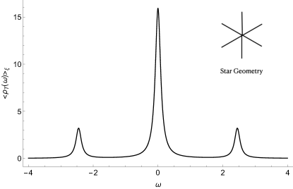
Figure 4: Plot of $\rho_{T}(\omega)$ against $\omega$ for star topology with 7 sites and $\gamma=0.1$. The central peak is 5 times more intense than each of the side peaks.

In the Supporting Information, we give results for a hexagonal unit of six sites.

In summary, we have shown that it is possible to find exact results for arbitrary one electron Hamiltonians with diagonal disorder, if the disorder has a Cauchy distribution. Using supersymmetric techniques, we showed that the the random terms in the Hamiltonian may be replaced by the non-random term $-i\gamma$ and the resultant complex Hamiltonian may be used to calculate averaged one-electron properties. Also, we showed that it is enough to diagonalize and find the eigenvalues of the Hamiltonian without any disorder, and then the results for all one particle properties for the disordered system may be obtained, avoiding the usual method of generating multiple realizations of the system, calculating the properties for each and then averaging them to get the averaged properties. Using the method, we report exact results for the disordered Tavis-Cummings Hamiltonian with arbitrary number of molecules. The solution shows the existence of two polaritonic states having a width which is half that of the distribution of the site energy on a given molecule. We pointed out that the width of the polaritonic peaks sensitively depend on the way the site energy is distributed. For a Gaussian distribution, the peaks narrow as the splitting increases, while for Cauchy is remains constant. As typical examples of other problems that could be solved exactly, we have also presented exact solutions for H$\ddot{u}$ckel type Hamiltonian, for an arrangement of sites having star topology. It is possible to use the method of this paper for any collection of sites with arbitrary topology. An interesting problem that remains is the analytical calculation of the inverse participation ratio (IPR). This requires calculation of the average of a product of two Green’s functions, and though the averaging can be done using the supersymmetric method, further progress seems difficult.

References

- Nagarajan et al. 2021 Nagarajan, K.; A, T.; W., E. T. Chemistry under Vibrational Strong Coupling. JACS 2021, 143, 16877
- Hartland and Scholes 2020 Hartland, G. V.; Scholes, G. Virtual Issue on Polaritons in Physical Chemistry. Journal of Physical Chemistry Letters 2020, 11, 7920
- Herrera and Owrutsky 2020 Herrera, F.; Owrutsky, J. Molecular polaritons for controlling chemistry with quantum optics. Journal of Chemical Physics 2020, 152, 100902
- Tavis and Cummings 1968 Tavis, M.; Cummings, F. W. Exact Solution for an N-Molecule-Radiation-Field Hamiltonian. Physical Review 1968, 170, 379–384
- Scholes 2020 Scholes, G. D. Polaritons and excitons: Hamiltonian design for enhanced coherence: Hamiltonian Design for Coherence. Proceedings of the Royal Society A: Mathematical, Physical and Engineering Sciences 2020, 476, 20200278
- Botzung et al. 2020 Botzung, T.; Hagenmuller, D.; Schutz, S.; Dubail, J.; Pupillo, G.; Schachenmayer, J. Dark state semilocalization of quantum emitters in a cavity. Physical Review B 2020, 102, 144202
- Du and Yuen-Zhou 2021 Du, M.; Yuen-Zhou, J. Can Dark States Explain Vibropolaritonic Chemistry? Arxiv 2021, http://arxiv.org/abs/2104.07214
- Sun et al. 2022 Sun, K.; Dou, C.; Gelin, M.; Zhao, Y. Dynamics of disordered Tavis–Cummings and Holstein–Tavis–Cummings models. Journal of Chemical Physics 2022, 156, 024102
- Houder et al. 1996 Houder, R.; Stanley, R. P.; Ilegems, M. Vacuum-field Rabi splitting in the presence of inhomogeneous broadening: Resolution of a homogeneous linewidth in an inhomogeneously broadened system. Physical Review A 1996, 53, 53
- Gera and Sebastian 2022 Gera, T.; Sebastian, K. L. Effects of disorder on polaritonic and dark states in a cavity using the disordered Tavis-Cummings model. arXiv:2202.06643 (quant-ph) 2022,
- Lloyd 1969 Lloyd, P. Exactly solvable model of electronic states in a three-dimensional disordered Hamiltonian: Non-existence of localized states. Journal of Physics C: Solid State Physics 1969, 2, 1717–1725
- Haake 2010 Haake, F. Quantum Signatures of Chaos; Springer, Heidelberg, 2010
- Zinn-Justin 2010 Zinn-Justin, J. Path Integrals in Quantum Mechanics; Sections 1.7 and 6.1.2; Oxford University Press, 2010