HINT: Hierarchical Neuron Concept Explainer

Abstract

To interpret deep networks, one main approach is to associate neurons with human-understandable concepts. However, existing methods often ignore the inherent relationships of different concepts (e.g., dog and cat both belong to animals), and thus lose the chance to explain neurons responsible for higher-level concepts (e.g., animal). In this paper, we study hierarchical concepts inspired by the hierarchical cognition process of human beings. To this end, we propose HIerarchical Neuron concepT explainer (HINT) to effectively build bidirectional associations between neurons and hierarchical concepts in a low-cost and scalable manner. HINT enables us to systematically and quantitatively study whether and how the implicit hierarchical relationships of concepts are embedded into neurons, such as identifying collaborative neurons responsible to one concept and multimodal neurons for different concepts, at different semantic levels from concrete concepts (e.g., dog) to more abstract ones (e.g., animal). Finally, we verify the faithfulness of the associations using Weakly Supervised Object Localization, and demonstrate its applicability in various tasks such as discovering saliency regions and explaining adversarial attacks. Code is available on https://github.com/AntonotnaWang/HINT.

1 Introduction

Deep neural networks have attained remarkable success in many computer vision and machine learning tasks. However, it is still challenging to interpret the hidden neurons in a human-understandable manner which is of great significance in uncovering the reasoning process of deep networks and increasing the trustworthiness of deep learning to humans [35, 68, 3].

Early research focuses on finding evidence from input data to explain deep model predictions [72, 38, 37, 57, 56, 60, 62, 59, 53, 31, 10, 4, 61], where the neurons remain unexplained. More recent efforts have attempted to associate hidden neurons with human-understandable concepts [80, 75, 76, 49, 50, 11, 7, 79, 9, 8, 23]. Although insightful interpretations of neurons’ semantics have been demonstrated, such as identifying the neurons controlling contents of trees [8], existing methods define the concepts in an ad-hoc manner, which heavily rely on human annotations such as manual visual inspection [80, 49, 50, 11], manually labeled classification categories [23], or hand-crafted guidance images [7, 79, 9, 8]. They thus suffer from heavy costs and scalability issues. Moreover, existing methods often ignore the inherent relationships among different concepts (e.g., dog and cat both belong to mammal), and treat them independently, which therefore loses the chance to discover neurons responsible for implicit higher-level concepts (e.g., canine, mammal, and animal) and explore whether the network can create abstractions of things like our humans do.

The above motivates us to rethink how concepts should be defined to more faithfully reveal the roles of hidden neurons. We draw inspirations from the hierarchical cognition process of human beings– human tend to organize things from specific to general categories [52, 67, 42]– and propose to explore hierarchical concepts which can be harvested from WordNet [44] (a lexical database of semantic relations between words). We investigate whether deep networks can automatically learn the hierarchical relationships of categories that were not labeled in the training data. More concretely, we aim to identify neurons for both low-level concepts such as Malamute, Husky, and Persian cat, and the implicit higher-level concepts such as dog and animal as shown in Figure 1 (a). (Note that we call less abstract concepts low-level and more abstract concepts high-level.)

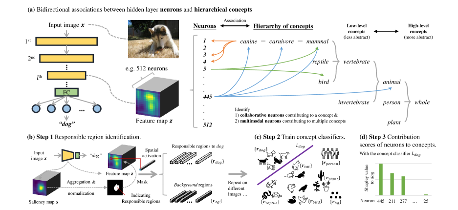
Figure 1: Overall illustration of HINT. (a) HINT is able to build bidirectional associations between hidden layer neurons and hierarchical concepts. It can also identify collaborative neurons and multimodal neurons. Further, HINT helps to indicate how the neurons learn the hierarchical relationships of categories. (b)-(c) Main steps. See Section 3.1 for Step 1, Section 3.2 for Step 2, and Section 3.3 for Step 3.

To this end, we develop HIerarchical Neuron concepT explainer (HINT) which builds a bidirectional association between neurons and hierarchical concepts (see Figure 1). First, we develop a saliency-guided approach to identify the high dimensional representations associated with the hierarchical concepts on hidden layers (noted as responsible regions in Figure 1 (b)), which makes HINT low-cost and scalable as no extra hand-crafted guidance is required. Then, we train classifiers shown in Figure 1 (c) to separate different concepts’ responsible regions where the weights represent the contribution of the corresponding neuron to the classification. Based on the classifiers, we design a Shapley value-based scoring method to fairly evaluate neurons’ contributions, considering both neurons’ individual and collaborative effects.

To our knowledge, HINT presents the first attempt to associate neurons with hierarchical concepts, which enables us to systematically and quantitatively study whether and how hierarchical concepts are embedded into deep network neurons. HINT identifies collaborative neurons contributing to one concept and multimodal neurons contributing to multiple concepts. Especially, HINT finds that, despite being trained with only low-level labels, such as Husky and Persian cat, deep neural networks automatically embed hierarchical concepts into its neurons. Also, HINT is able to discover responsible neurons to both higher-level concepts, such as animal, person and plant, and lower-level concepts, such as mammal, reptile and bird.

Finally, we verify the faithfulness of neuron-concept associations identified by HINT with a Weakly Supervised Object Localization task. In addition, HINT achieves remarkable performance in a variety of applications, including saliency method evaluation, adversarial attack explanation, and COVID19 classification model evaluation, further manifesting the usefulness of HINT.

2 Related Work

Neuron-concept Association Methods. Neuron-concept association methods aim at directly interpreting the internal computation of CNNs [12, 2, 25, 48]. Early works show that neurons on shallower layers tend to learn simpler concepts, such as lines and curves, while higher layers tend to learn more abstract ones, such as heads or legs [72, 71]. TCAV [32] and related studies [22, 24] quantify the contribution of a given concepts represented by guidance images to a target class on a chosen hidden layer. Object Detector [80] visualizes the concept-responsible region of a neuron in the input image by iteratively simplifying the image. After that, Network Dissection [7, 79, 8] quantifies the roles of neurons by assigning each neuron to a concept with the guidance of extra images. GAN Dissection [9, 8] illustrates the effect of concept-specific neurons by altering them and observing the emergence and vanishing of concept-related contents in images. Neuron Shapley [23] identifies the most influential neuron over all hidden layers to an image category by sorting Shapley values [54]. Besides pre-defined concepts, feature visualization methods [49, 50, 11] generate Deep Dream-style [47] explanations for each neuron and manually interpret their meanings. Additionally, Net2Vec [20] maps semantic concepts to vectorial embeddings to investigate the relationship between CNN filters and concepts. However, existing methods cannot systematically explain how the network learns the inherent relationships of concepts, and suffer from high cost and scalability issues. HINT is proposed to overcome the limitations and goes beyond exploring each concept individually – it adopts hierarchical concepts to explore their semantic relationships.

Saliency Map Methods. Saliency map methods are a stream of simple and fast interpretation methods which show the pixel responsibility (i.e. saliency score) in the input image for a target model output. There are two main categories of saliency map methods – backpropagation-based and perturbation-based. Backpropagation-based methods mainly generate saliency maps by gradients; they include Gradient [57], Gradient x Input [56], Guided Backpropagation [60], Integrated Gradient [62], SmoothGrad [59], LRP [5, 26], Deep Taylor [46], DeepLIFT [55], and Deep SHAP [13]. Perturbation-based saliency methods perturbate input image pixels and observe the variations of model outputs; they include Occlusion [72], RISE [51], Real-time [15], Meaningful Perturbation [21], and Extremal Perturbation [19]. Inspired by saliency methods, in HINT, we build a saliency-guided approach to identify the responsible regions for each concept on hidden layers.

3 Method

Overview. Considering a CNN classification model $f$ and a hierarchy of concepts $\mathcal{E}:\{e\}$ (see Figure 1 (a)), our goal is to identify bidirectional associations between neurons and hierarchical concepts. To this end, we develop HIerarchical Neuron concepT explainer (HINT) to quantify the contribution of each neuron $d$ to each concept $e$ by a contribution score $\phi$ where higher contribution value means stronger association between $d$ and $e$, and vice versa.

The key problem therefore becomes how to estimate the score $\phi$ for any pair of $e$ and $d$. We achieve this by identifying how the network map concept $e$ to a high dimensional space and quantifying the contribution of $d$ for the mapping. First, given a concept $e$ and an image $x$, on feature map $z$ of the $l^{th}$ layer, HINT identifies the responsible regions $\mbox{\boldmath$r$}_{e}$ to concept $e$ by developing a saliency-guided approach elaborated in Section 3.1. Then, given the identified regions for all the concepts, HINT further trains concept classifier $L_{e}$ to separate concept $e$’s responsible regions $\mbox{\boldmath$r$}_{e}$ from other regions $\mbox{\boldmath$r$}_{\mathcal{E}\backslash e}\cup\mbox{\boldmath$r$}_{b^{*}}$ where $b^{*}$ represents background (see Section 3.2). Finally, to obtain $\phi$, we design a Shapley value-based approach to fairly evaluate the contribution of each neuron $d$ from the concept classifiers (see Section 3.3).

Input: A set of images with hierarchical concepts $\{(\mbox{\boldmath$x$},e)\}$, a set of neurons $\mathcal{D}$ for experiment, modified saliency method $\Lambda$, aggregation method $\zeta$, and threshold $t\in(0,10$.

Output: Score matrix $\Phi$ where every element $\phi$ is the Shapely value of neuron $d$ to concept $e$.

Init: Responsible region containers $\mbox{\boldmath$r$}_{e}=\{\ \}$ for each $e$ in $\mathcal{E}$, background region container $\mbox{\boldmath$r$}_{b^{*}}=\{\ \}$, and score matrix $\Phi=\{0\}^{|\mathcal{D}|\times|\mathcal{E}|}$.

1

2for each $(\mbox{\boldmath$x$},e)$ do

3       feature map $\mbox{\boldmath$z$}=f_{l}(\mbox{\boldmath$x$})$ ;

4       saliency map $\mbox{\boldmath$s$}=\Lambda(\mbox{\boldmath$x$},f_{l}\ |\ e)$ ;

5       $\mbox{\boldmath$z$}\leftarrow\mbox{\boldmath$z$}_{\mathcal{D},:,:}$ ;

6       $\mbox{\boldmath$s$}\leftarrow\mbox{\boldmath$s$}_{\mathcal{D},:,:}$ ;

7       $\hat{\mbox{\boldmath$s$}}=Normalization(\zeta(\mbox{\boldmath$s$}))\in[0,1]^{H_{l}\times W_{l}}$ ;

8       $\mbox{\boldmath$z$}_{e}=\mbox{\boldmath$z$}\odot(\hat{\mbox{\boldmath$s$}}\geq t)$, add $\mbox{\boldmath$z$}_{e}$ to $\mbox{\boldmath$r$}_{e}$ ;

9       $\mbox{\boldmath$z$}_{b^{*}}=\mbox{\boldmath$z$}\odot(\hat{\mbox{\boldmath$s$}}<t)$, add $\mbox{\boldmath$z$}_{b^{*}}$ to $\mbox{\boldmath$r$}_{b^{*}}$ ;

10      

11for each $e$ in $\mathcal{E}$ do

12       Train classifier $L_{e}$ which separates $\mbox{\boldmath$r$}_{e}$ and $\mbox{\boldmath$r$}_{\mathcal{E}\backslash e}\cup\mbox{\boldmath$r$}_{b^{*}}$

13for each $e$ in $\mathcal{E}$ do

14       for each $d$ in $\mathcal{D}$ do

15             $\phi=$ Shapley value of neuron $d$ to concept $e$;

16             Update $\Phi$ with $\phi$;

17            

18      

Algorithm 1 HINT

3.1 Responsible Region Identification for Concepts

In this section, we introduce our saliency-guided approach to collect the responsible regions $\mbox{\boldmath$r$}_{e}$ for a certain concept $e\in\mathcal{E}$ to serve as the training samples of the concept classifier which will be described in Section 3.2.

Taking an image $x$ containing a concept $e$ as input, the network $f$ generates a feature map $\mbox{\boldmath$z$}\in\mathbb{R}^{D_{l}\times H_{l}\times W_{l}}$ where there are $D_{l}$ neurons in total. Generally, not all regions of $z$ are equally related to $e$ [76]. In other words, some regions have stronger correlations with $e$ while others are less correlated, as shown in Figure 1 (b) “Step 1”. Based on the above observation, we propose a saliency-guided approach to identify the closely related regions $\mbox{\boldmath$r$}_{e}$ to the concept $e$ in feature map $z$. We call them responsible regions.

First, we obtain the saliency map on the $l^{th}$ layer. As shown in Figure 1 (b) “Step 1”, with the feature map $z$ on the $l^{th}$ layer extracted, we derive the $l^{th}$ layer’s saliency map $s$ with respect to concept $e$ by the saliency map estimation approach $\Lambda$. Note that HINT is compatible with different back-propagation based saliency map estimation methods. We implement five of them [57, 56, 60, 62, 59], please refer to the Supplementary Material for more details. Note that different from existing works [57, 56, 60, 62, 59] that pass the gradients to the input image as saliency scores, we early stop the back-propagation at the $l^{th}$ layer to obtain the saliency map $s$. Here, we use modified SmoothGrad [59] as an example to demonstrate our approach: $\textstyle\Lambda=\frac{1}{N}\sum_{n=1}^{N}\frac{\partial f^{e}(\mbox{\boldmath$x$}^{{}^{\prime}})}{\partial\mbox{\boldmath$z$}^{{}^{\prime}}}$ where $\textstyle\mbox{\boldmath$x$}^{{}^{\prime}}=\mbox{\boldmath$x$}+\mathcal{N}(\mu,\sigma^{2}_{n})$ and $\mathcal{N}$ indicates normal distribution. It is notable that we may also optimally select part of the neurons $\mathcal{D}$ for analysis.

Next is to identify the responsible regions on feature map $z$ with the guidance of the saliency map $s$. Specifically, we categorize each entry $z_{\mathcal{D},i,j}$ in $z$ to be responsible to $e$ or not. To this end, the saliency map $s$ is first aggregated by an aggregation function $\zeta$ along the channel dimension and then normalized to be within $[0,1]$. Note that different aggregation functions $\zeta$ can be applied (see five different $\zeta$ shown in Supplementary Material). Here, we aggregate $s$ using Euclidean norm $\textstyle\zeta=\|\mbox{\boldmath$s$}\|$ along its first dimension. After that, we obtain $\hat{\mbox{\boldmath$s$}}\in[0,1]^{H_{l}\times W_{l}}$ with each element $s_{i,j}$ indicating the relevance of $z_{\mathcal{D},i,j}$ to concept $e$. By setting a threshold $t$ ( we set $t$ as $0.5$ in the paper) and masking $z$ with $\hat{\mbox{\boldmath$s$}}\geq t$ and $\hat{\mbox{\boldmath$s$}}<t$, we finally obtain responsible regions and background regions respectively (see the illustration of the two regions Figure 1 (b): “Step 1”).

Our saliency-guided approach extends the interpretability of saliency methods, which originally aim to find the “responsible regions” to a concept on one particular image. However, our approach is able to identify “responsible regions” to a concept on the high dimensional space of a hidden layer from multiple images, which can more accurately describe how the network represents concept $e$ internally. Therefore, our saliency-guided approach provides better interpretability as it helps us to investigate the internal abstraction of concept $e$ in the network.

3.2 Training of Concept Classifiers

For all images, we identify its responsible regions for each concept $e\in\mathcal{E}$ following the procedures described in 3.1 and construct a dataset which contains a collection of responsible regions $\mbox{\boldmath$r$}_{e}$ and a collection of background regions $\mbox{\boldmath$r$}_{b^{*}}$. Given the dataset, as shown in Figure 1 (c) “Step 2”, we use the high dimensional CNN hidden layer features to train a concept classifier $L_{e}$ which distinguishes $\mbox{\boldmath$r$}_{e}$ from $\mbox{\boldmath$r$}_{\mathcal{E}\backslash e}\cup\mbox{\boldmath$r$}_{b^{*}}$, i.e., separating concept $e$ from other concepts ${\mathcal{E}\backslash e}\cup{b^{*}}$ (Line 9 and 10 in Algorithm 1).

$L_{e}$ can have many forms: a linear classifier, a decision tree, a Gaussian Mixture Model, and so on. Here, we use the simplest form, a linear classifier, which is equivalent to a hyperplane separating concept $e$ from others in the high dimensional feature space of CNN.

$$L_{e}(r)=\sigma\left(\mbox{\boldmath$\alpha$}^{T}r\right),$$ (1)

where $r=z_{\mathcal{D},i,j}\in\mathbb{R}^{|\mathcal{D}|}$ represents spatial activation with each element representing a neuron; $\alpha$ is a vector of weights, $\sigma$ is a sigmoid function, and $L_{e}(r)\in[0,1]$ represents the confidence of $r$ related to a concept $e$.

It is notable that we can apply the concept classifier $L_{e}$ back to the feature map $z$ to visualize how $L_{e}$ detect concept $e$. Classifiers of more abstract concepts (e.g., whole) tend to activate regions of more general features, which helps us to locate the entire extent of the object. On contrary, classifiers of lower-level concepts tend to activate regions of discriminative features such as eyes and heads.

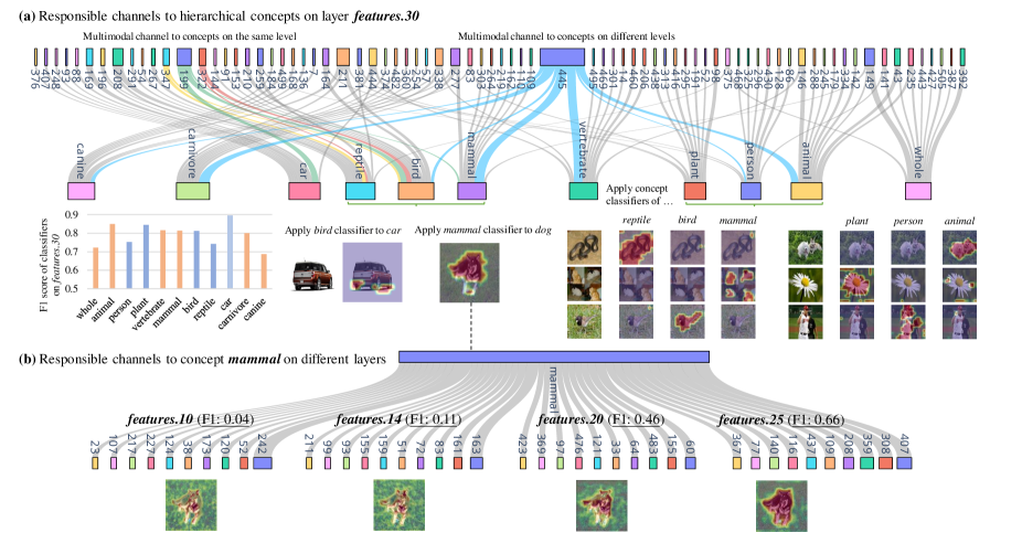
Figure 2: Bidirectional associations between neurons and hierarchical concepts. The width of the link indicates the size of the contribution score of a neuron to a concept. (a) Responsible neurons to hierarchical concepts (see the hierarchy in Figure 1) on layer features.30 in VGG19. The F1 scores of concept classifiers show their capability of distinguishing the target concepts. The pictures illustrate the results of applying concept classifiers on different images. For most of the cases, the concept classifiers only locate the objects belonging to the target concepts. However, as bird and car share multimodal neurons, the bird classifier responses to the wheels of the car. (b) Responsible neurons to mammal on different layers. The pictures and F1 scores indicate the network can more easily distinguish mammal from other concepts as the layer goes higher.

3.3 Contribution Scores of Neurons to Concepts

Next is to decode the contribution score $\phi$ from the concept classifiers. A simple method to estimate $\phi$ is to use the learned classifier weights corresponding to each neuron $e$, where a higher value typically means a larger contribution [45]. However, the assumption that $\alpha$ can serve as the contribution score is that the neurons are independent of each other, which is generally not true. To achieve a fair evaluation of neurons’ contributions to $e$, a Shapley value-based approach is designed to calculate the scores $\phi$, which can take account of neurons’ individual effects as well as the contributions coming from the collaboration with others.

Shapely value [54] is from Game Theory, which evaluates channels’ individual and collaborative effects. More specifically, if a channel cannot be used for classification independently but can greatly improve classification accuracy when collaborating with other channels, its Shapley value can still be high. Shapely value satisfies the properties of efficiency, symmetry, dummy, and additivity [45]. Monte-Carlo sampling is used to estimate the Shapley values by testing the target neuron’s possible coalitions with other neurons. Equation (2) shows how we calculate Shapley value $\phi$ of a neuron $d$ to concept $e$.

$$\phi=\frac{\sum_{\mbox{\boldmath$r$}}\left|\sum_{i=1}^{M}\left(L_{e}^{\langle\mathcal{S}\cup d\rangle}(r)-L_{e}^{\langle\mathcal{S}\rangle}(r)\right)\right|}{M|\mbox{\boldmath$r$}_{\mathcal{E}}\cup\mbox{\boldmath$r$}_{b^{*}}|}$$ (2)

where $r=z_{\mathcal{D},i,j}$ represents spatial activation from $\mbox{\boldmath$r$}_{\mathcal{E}}$ and $\mbox{\boldmath$r$}_{b^{*}}$; $\textstyle\mathcal{S}\subseteq\mathcal{D}\backslash d$ is the neuron subset randomly selected at each iteration; $\textstyle\langle*\rangle$ is an operator keeping the neurons in the brackets, i.e., $\mathcal{S}\cup d$ or $\mathcal{S}$, unchanged while randomizing others; $M$ is the number of iterations of Monte-Carlo sampling; $L_{e}^{\langle*\rangle}$ means that the classifier is re-trained with neurons in the brackets unchanged and others being randomized.

By repeating the calculation for different $e$ and $d$ (see Line 11 to line 14 in Algorithm 1), finally, we can get the score matrix $\Phi$.

3.4 Neuron-Concept Association

By repeating the score calculations for all pairs of $e$ and $d$, we obtain a score matrix $\Phi$ where each row represents a neuron $d$ and each column represents a concept $e$ in the hierarchy. By sorting the scores in the column of concept $e$, we can get collaborative neurons all having high contributions to a concept $e$. Also, by sorting the scores in the row of neuron $d$, we can test whether $d$ is multimodal (having high scores to multiple concepts) and observe a hierarchy of concepts that $d$ is responsible for.

Note that the score matrix $\Phi$ cannot tell us the exact number of responsible neurons to concept $e$. For a contribution score $\phi$ which is zero or near zero, the corresponding neuron $d$ can be regarded as irrelevant to the corresponding concept $e$. Therefore, for truncation, we may set a threshold for $\phi$. In our experiment, for a concept, we sort scores and select the top $N$ as responsible neurons.

4 Experiments

4.1 Experimental setup

HINT is a general framework which can be applied on any CNN architectures. We evaluate HINT on several models trained on ImageNet [17] with representative CNN backbones including VGG-16 [58], VGG-19 [58], ResNet-50 [27], and Inception-v3 [63]. In this paper, the layer names are from PyTorch pretrained models (e.g., “features.30” is a layer name of VGG19). The hierarchical concept set $\mathcal{E}$ is built upon the $1000$ categories of ImageNet with hierarchical relationship is defined by WordNet [44] as shown in Figure 1. Figure 3 shows the computational complexity analysis, indicating that Shapely value calculation is negligible when considering the whole cycle.

4.2 Responsible Neurons to Hierarchical Concepts

In this section, we study the responsible neurons for the concepts and show the hierarchical cognitive pattern of CNNs. We adopt the VGG-19 backbone and show the top-10 significant neurons to each concept ($N$=10). The results in Figure 2 manifest that HINT explicitly reveals the hierarchical learning pattern of the network: some neurons are responsible to concepts with higher semantic levels such as whole and animal, and others are responsible to more detailed concepts such as canine. Besides, HINT shows that there can be multiple neurons contributing to a single concept and HINT identifies multimodal neurons which have high contributions to multiple concepts.

Concepts of different levels. First, we investigate the concepts of different levels in Figure 2 (a). Among all the concepts, whole has the highest semantic level including animal, person, and plant. To study how a network recognizes a Husky (a subclass of canine) image on a given layer, HINT hierarchically identifies the neurons which are responsible for the concept from higher levels (like whole, animal) to lower ones (like canine). Besides, HINT is able to identify multimodal neurons which take responsibility to many concepts at different semantic levels. For example, the $445^{th}$ neuron delivers the most contribution to multiple concepts including animal, vertebrate, mammal, and carnivore, and also contributes to canine, manifesting that the $445^{th}$ neuron captures the general and specie-specific features which are not labeled in the training data.

Concepts of the same level. Next, we study the responsible neurons for concepts at the same level identified by HINT. For mamml, reptile, and bird, there exist multimodal neurons as the three categories share morphological similarities. For example, the $199^{th}$ and $445^{th}$ neurons contribute to both mammal and bird, while the $322^{nd}$ and $347^{th}$ neurons are individually responsible for both reptile and bird. Interestingly, HINT identifies multimodal neurons contributing to concepts which are conceptually far part to humans. For example, the $199^{th}$ neuron contributes to both bird and car. By applying the bird classifier to images of bird and car, we find that the body of the bird and the wheels of the car can be both detected.

Same concept on different layers. We also identify responsible neurons on different network layers with HINT. Figure 2 (b) illustrates the 10 most responsible neurons to mammal in other four network layers. On shallow layers, such as on layer features.10, HINT indicates that the concept of mammal cannot be recognized by the network (F1 score: 0.04). However, as the network goes deeper, the F1 score of mammal classifier increases until around 0.8 on layer features.30, which is consistent with the existing works [72, 71] that deeper layers capture higher-level and richer semantic meaningful features.

Figure 3: Time consumption for different stages of HINT. The most time consuming part is the data preparation process. Shapely value computation takes about $5$ minutes with a single NVIDIA RTX 2080, while linear classifier training takes $1-3$ minutes. Therefore, the time consumption of Shapely value calculation is negligible when considering the whole cycle.

4.3 Verification of Associations by Weakly Supervised Object Localization

With the associations between neurons and hierarchical concepts obtained by HINT, we further validate the associations using Weakly Supervised Object Localization (WSOL). Specifically, we train a concept classifier $L_{e}$ (see detailed steps in Section 3.1 and 3.2) with the top-$N$ significant neurons corresponding to concept $e$ at a certain layer, and locate the responsible regions using $L_{e}$ as the localization results. Good localization performance of $L_{e}$ indicates the $N$ neurons also have high contributions to concept $e$.

Comparison of localization accuracy. Quantitative evaluation in Table 1 and 2 show that HINT achieves comparable performance with existing WSOL approaches, thus validating the associations. We train animal (Table 1) and whole (Table 2) classifiers with 10%, 20%, 40%, 80% neurons sorted and selected by Shapley values on layer “features.26” (512 neurons) of VGG16, layer “layer3.5” (1024 neurons) of ResNet50, and layer “Mixed_6b” (768 neurons) of Inception v3, respectively. To be consistent with the commonly-used WSOL metric, Localization Accuracy measures the ratio of images with IoU of groundtruth and predicted bounding boxes larger than 50%. In Table 1, we compare HINT with the state-of-the-art methods on dataset CUB-200-2011 [65], which contains images of 200 categories of birds. Note that existing localization methods need to re-train the model on the CUB-200-2011 as they are tailored to the classifier while HINT directly adopts the classifier trained on ImageNet without further finetuning on CUB-200-2011. Even so, HINT still achieves a comparable performance when adopting VGG16 and Inception v3, and performs the best when adopting ResNet50. However, Table 2 shows that HINT outperforms all existing methods on all models on ImageNet. Besides, the differences of localization accuracy may indicate different models have different learning modes. Precisely, few neurons in VGG16 are responsible for animal or whole while most neurons in ResNet50 contribute to identifying animal or whole. In conclusion, the results quantitatively prove that the associations are valid and HINT achieves comparable performance to WSOL. More analysis is included in the supplementary file.

Table 1: Comparison of Localization Accuracy on CUB-200-2011. * indicates fine-tuning on CUB-200-2011.

	VGG16	ResNet50	Inception v3
CAM* [81]	34.4%	42.7%	43.7%
ACoL* [77]	45.9%	-	-
SPG* [78]	-	-	46.6%
ADL* [14]	52.4%	62.3%	53.0%
DANet* [69]	52.5%	-	49.5%
EIL* [41]	57.5%	-	-
PSOL* [73]	66.3%	70.7%	65.5%
GCNet* [36]	63.2%	-	-
RCAM* [6]	59.0%	59.5%	-
FAM* [43]	69.3%	73.7%	70.7%
Ours (10%)	66.6%	60.2%	49.0%
Ours (20%)	65.2%	67.1%	55.8%
Ours (40%)	61.3%	77.3%	52.8%
Ours (80%)	64.8%	80.2%	56.2%

Table 2: Comparison of Localization Accuracy on ImageNet.

	VGG16	ResNet50	Inception v3
CAM [81]	42.8%	-	-
ACoL [77]	45.8%	-	-
SPG [78]	-	-	48.6%
ADL [14]	44.9%	48.5%	48.7%
DANet [69]	-	-	48.7%
EIL [41]	46.8%	-	-
PSOL [73]	50.9%	54.0%	54.8%
GCNet [36]	-	-	49.1%
RCAM [6]	44.6%	49.4%	-
FAM [43]	52.0%	54.5%	55.2%
Ours (10%)	64.7%	59.7%	53.1%
Ours (20%)	66.1%	66.6%	54.1%
Ours (40%)	64.4%	69.4%	54.3%
Ours (80%)	62.6%	70.7%	58.7%

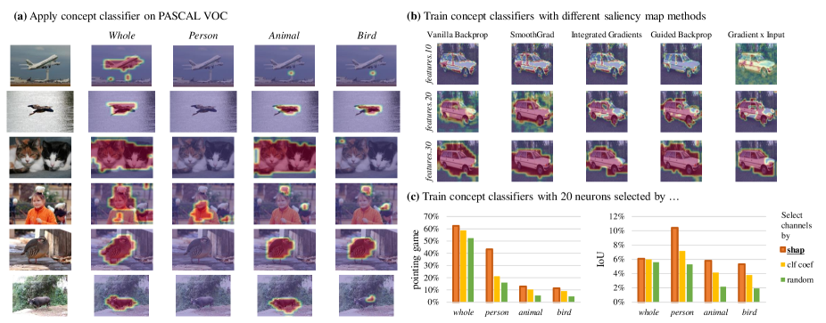
Figure 4: Results of Weakly Supervised Object Localization and ablation study. (a) Illustration of applying different concept classifiers on PASCAL VOC 2007, showing that HINT can locate objects of chosen concepts. (b) Ablation study showing the results of different saliency methods. (c) Ablation study showing Shapley values are good measures of neurons’ contributions. The concept classifiers are trained with 20 neurons selected by different approaches. The pointing game (mask intersection over the groundtruth mask) and IoU (mask intersection over union of masks) scores show the accuracy of whole, person, animal, and bird concept classifiers on PASCAL VOC 2007.

Flexible choice of localization targets. When locating objects, HINT has a unique advantage: a flexible choice of localization targets. We can locate objects on different levels in the concept hierarchy (e.g., bird, mammal, and animal). In experiments, we train concept classifiers of whole, person, animal, and bird using 20 most important neurons on layer features.30 of VGG19 and apply them on PASCAL VOC 2007 [18]. Figure 4 (a) shows that HINT can accurately locate the objects belonging to different concepts.

Extension to locate the entire extent of the object. Many existing WSOL methods adapt the model architecture and develop training techniques to highlight the entire extent rather than discriminative parts of object [69, 41, 73, 36, 6, 43]. However, can we effectively achieve this goal without model adaptation and retraining? HINT provid es an approach to utilize the implicit concepts learned by the model. As shown in Figure 4 (c), classifiers of higher-level concepts (e.g. whole) tend to draw larger masks on objects than classifiers of lower-level concepts (e.g. bird). It is because that the responsible regions of whole contain all the features of its subcategories. Naturally, the whole classifier tends to activate full object regions rather than object parts.

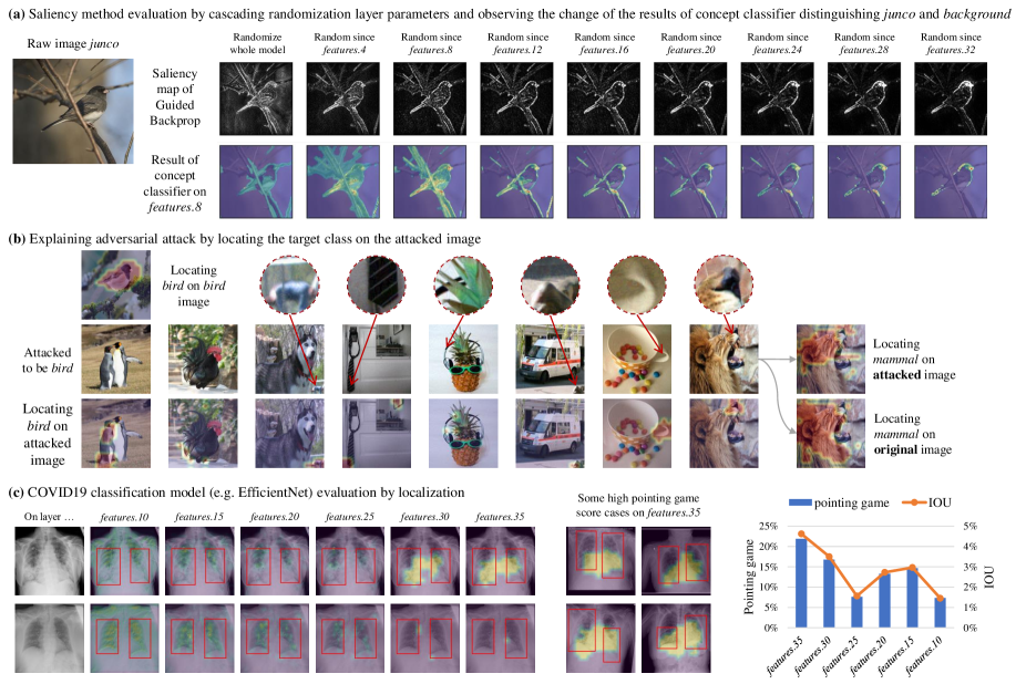
Figure 5: Other applications of HINT. (a) Saliency method evaluation. (b) Explaining adversarial attack. (c) COVID19 classification model evaluation.

4.4 Ablation Study

We perform an ablation study to show that HINT is general and can be implemented with different saliency methods, and Shapley values are good measures of neurons’ contributions to concepts.

Implementation with different saliency methods. We train concept classifiers with five modified saliency methods (see Supplementary Material). Then, we apply the classifiers to the object localization task. Figure 4 (b) shows that the five saliency methods all perform well. This shows that HINT is general, and different saliency methods can be integrated into HINT,

Shapley values. To test the effectiveness of Shapley values, we train concept classifiers using 20 neurons on layer features.30 of VGG19 by different selection approaches, including Shapley values (denoted as shap), absolute values of linear classifier coefficients (denoted as clf_coef), and random selection (denoted as random). We then use the classifiers to perform localization tasks on PASCAL VOC 2007 (see Figure 4 (c)). Two metrics are used: pointing game (mask intersection over the groundtruth mask, usually used by other interpretation methods) [74] and IoU (mask intersection over the union of masks). The results show that “shap” outperforms “clf_coef” and “random” when locating different targets. This suggests that Shapley value is a good measure of neuron contribution as it considers both the individual and collaborative effects of neurons. On contrary, linear classifier coefficients assume that neurons are independent of each other.

4.5 More Applications

We further demonstrate HINT’s usefulness and extensibility by saliency method evaluation, adversarial attack explanation, and COVID19 classification model evaluation (Figure 5). Please refer to Supplementary Material for detailed descriptions.

Saliency method evaluation. Guided Backpropagation can pass the sanity test in [1, 30] if we observe the hidden layer results (see Figure 5 (a)). On layer features.8, with less randomized layers, the classifier-identified regions are more concentrated on the key features of the bird – its beak and tail, thereby suggesting that Guided Backpropagation detects the salient regions.

Explaining adversarial attack. We attack images of various classes to be bird using PGD [40] and apply the bird classifier to their feature map. The responsible regions for concept bird highlighted in those fake bird images may imply that, for certain images, adversarial attack does not change the whole body of the object to be another class but captures some details of the original image, where there exist shapes similar to bird (see Figure 5 (b)). For example, in the coffee mug image where most shapes are round, adversarial attack catches the only pointed shape and attacks it to be like bird. Upon above observations, we design a quantitative evaluation on the faithfulness of our explanations. First, we attack 300 images of other categories excluding bird to be birds based on VGG19 model. Then, we use a bird classifier to find the regions corresponding to the adversarial features of bird on the attacked images. By visual inspection, we find most regions contain point shapes. Based on the regions, we train an adversarial attacked “bird” classifier (“ad clf”). Finally, we use the “ad clf” to perform the WSOL task on real bird images. The accuracy is 64.3% (for true bird classifier, it is 70.1%), indicating HINT captures the adversarial bird features and validates the explanation: some kind of adversarial attacks may be caused by attacking the similar shapes of the target class.

COVID19 classification model evaluation Applying deep learning to the detection of COVID19 in chest radiographs has the potential to provide quick diagnosis and guide management in molecular test resource-limited situations. However, the robustness of those models remains unclear [16]. We do not know whether the model decisions rely on confounding factors or medical pathology in chest radiographs. Object localization with HINT can check whether the identified responsible regions overlap with the lesion regions drawn by doctors (see Figure 5 (c)). As you can see, the pointing game and IoU are not high. Many cases having low pointing game and IoU values show that the model does not focus on the lesion region, while for the cases with high pointing game and IoU values, further investigation is still required to see whether they capture the medical pathology features or they just accidentally focus on the area of the stomach.

5 Limitations of Interpretations

HINT can systematically and quantitatively identify the responsible neurons to implicit high-level concepts. However, our approach cannot handle concepts that are not included in the concept hierarchy. And it is not effective to identify responsible neurons to concepts lower than the bottom level of the hierarchy which are the classification categories. More explorations are needed if we want to build such neuron-concept associations.

6 Conclusion

We have presented HIerarchical Neuron concepT explainer (HINT) method which builds bidirectional associations between neurons and hierarchical concepts in a low-cost and scalable manner. HINT systematically and quantitatively explains whether and how the neurons learn the high-level hierarchical relationships of concepts in an implicit manner. Besides, it is able to identify collaborative neurons contributing to the same concept but also the multimodal neurons contributing to multiple concepts. Extensive experiments and applications manifest the effectiveness and usefulness of HINT. We open source our development package and hope HINT could inspire more investigations in this direction.

7 Acknowledgments

This work has been supported in part by Hong Kong Research Grant Council - Early Career Scheme (Grant No. 27209621), HKU Startup Fund, and HKU Seed Fund for Basic Research. Also, we thank Mr. Zhengzhe Liu for his insightful comments and careful editing of this manuscript.

Supplementary File

In this supplementary file, first, we show the five modified saliency methods and five aggregation approaches with which HINT can be implemented in Section A and B respectively. Second, we explain the properties that HINT’s Shapley value-based neuron contribution scoring approach satisfies in Section C. Third, we provide detailed descriptions of applications of HINT – saliency method evaluation, explaining adversarial attack, and evaluation of COVID19 classification models – in Section D. Next, we demonstrate more neuron-concept associations and the activation maps of multimodal neurons in Section E. Then, we show more quantitative analysis and illustrations of the results of applying HINT for Weakly Supervised Object Localization tasks in Section F. Finally, we provide more illustrations of ablation studies on modified saliency methods and Shapley value-based scoring approach in Section G.

Appendix A Modified Saliency Methods

Table S.1: Modified saliency methods and aggregation approaches

Modified saliency methods $\Lambda$ on the $l^{th}$ layer with respect to concept $e$		Aggregation approaches $\zeta$
Vanilla Backpropagation [57]	$\textstyle\frac{\partial f^{e}(\mbox{\boldmath$x$})}{\partial\mbox{\boldmath$z$}}$	Norm	$\textstyle\|\mbox{\boldmath$s$}\|$
Gradient x Input [56]	$\textstyle\mbox{\boldmath$z$}\odot\frac{\partial f^{e}(\mbox{\boldmath$x$})}{\partial\mbox{\boldmath$z$}}$	Filter norm	$\textstyle\left\|\mbox{\boldmath$s$}>0\odot\mbox{\boldmath$s$}\right\|$
Guided Backpropagation [60]	$\textstyle\left(\frac{\partial f^{e}(\mbox{\boldmath$x$})}{\partial\mbox{\boldmath$z$}}\right)_{l+1}>0\odot\frac{\partial f^{e}(\mbox{\boldmath$x$})}{\partial\mbox{\boldmath$z$}}$	Max	$\textstyle\max(\mbox{\boldmath$s$})$
Integrated Gradient [62]	$\textstyle f_{l}(\mbox{\boldmath$x$}-\bar{\mbox{\boldmath$x$}})\odot\int_{0}^{1}\frac{\partial f^{e}(\mbox{\boldmath$x$}+\alpha(\mbox{\boldmath$x$}-\bar{\mbox{\boldmath$x$}}))}{\partial\mbox{\boldmath$z$}}\ d\alpha$	Abs max	$\textstyle\max(|\mbox{\boldmath$s$}|)$
SmoothGrad [59]	$\textstyle\frac{1}{N}\sum_{n=1}^{N}\frac{\partial f^{e}(\mbox{\boldmath$x$}^{{}^{\prime}})}{\partial\mbox{\boldmath$z$}^{{}^{\prime}}},\mbox{\boldmath$x$}^{{}^{\prime}}=\mbox{\boldmath$x$}+\mathcal{N}(\mu,\sigma^{2}_{n})$	Abs sum	$\textstyle\sum(|\mbox{\boldmath$s$}|)$

Inspired by backpropagation-based saliency methods, we develop a saliency-guided approach to identify responsible regions in feature map $z$. Equation (S.1) shows how the representative backpropagation-based saliency method, Gradient (Vanilla Backpropagation) [57], calculates the contribution of pixel $\mbox{\boldmath$x$}_{:,i_{0},j_{0}}$ to a class $C_{k}$.

$$\frac{\partial f^{C_{k}}(\mbox{\boldmath$x$})}{\partial\mbox{\boldmath$x$}_{:,i_{0},j_{0}}}$$ (S.1)

where $f$ is a deep network, $f^{C_{k}}(\mbox{\boldmath$x$})$ is the logit of $x$ to class $C_{k}$, and $\mbox{\boldmath$x$}_{:,i_{0},j_{0}}$ is a pixel.

We extend the idea of saliency maps to hidden layers. We take concept $e$ and neurons $\mathcal{D}$ on the $l^{th}$ layer as an example. Given an image $x$ with label $C_{k}$ where $C_{k}$ is concept $e$ or a subcategory of concept $e$, the contribution of spatial activation $\mbox{\boldmath$z$}_{\mathcal{D},i_{l},j_{l}}$ to class $C_{k}$ (also to concept $e$) is shown in Equation (S.2)

$$\mbox{\boldmath$s$}_{\mathcal{D},i_{l},j_{l}}=\frac{\partial f^{C_{k}}(\mbox{\boldmath$z$})}{\partial\mbox{\boldmath$z$}_{\mathcal{D},i_{l},j_{l}}}$$ (S.2)

where $\mbox{\boldmath$s$}_{\mathcal{D},i_{l},j_{l}}\in\mathbb{R}^{|\mathcal{D}|}$ is a vector and $\mbox{\boldmath$s$}_{\mathcal{D},i_{l},j_{l}}$s for each $i_{l}$ and $j_{l}$ form the saliency map $s$.

As shown in Table S.1, we modify five backpropagation-based saliency methods. All of them can be used in HINT.

Appendix B Aggregation Approaches

With saliency map $s$, the next step is to aggregate $\mbox{\boldmath$s$}_{\mathcal{D},i_{l},j_{l}}$, and the aggregated value will be used to decide whether $\mbox{\boldmath$z$}_{\mathcal{D},i_{l},j_{l}}$s belong to responsible foreground regions or irrelevant background regions. We implement five aggregation approaches shown in Table S.1. All of them can be applied to HINT. Note that the aggregation is only conducted along the first dimension of $s$.

Appendix C Properties of HINT’s Shapley Value-based Neuron Contribution Scoring Approach

In the main paper, the Shapley value $\phi$ of a neuron $d$ to a concept $e$ is calculated as Equation (S.3).

$$\phi=\frac{\sum_{\mbox{\boldmath$r$}}\left|\sum_{i=1}^{M}\left(L_{e}^{\langle\mathcal{S}\cup d\rangle}(r)-L_{e}^{\langle\mathcal{S}\rangle}(r)\right)\right|}{M|\mbox{\boldmath$r$}_{\mathcal{E}}\cup\mbox{\boldmath$r$}_{b^{*}}|}$$ (S.3)

where $\mathcal{D}$ is the set of neurons; $L_{e}$ is the classifier for concept $e$; $r=z_{\mathcal{D},i,j}$ represents spatial activation; $\mbox{\boldmath$r$}_{\mathcal{E}}$ and $\mbox{\boldmath$r$}_{b^{*}}$ are responsible regions of all concept $e\in\mathcal{E}$ and background regions; $\textstyle\mathcal{S}\subseteq\mathcal{D}\backslash d$ is the neuron subset randomly selected at each iteration; $\textstyle\langle*\rangle$ is an operator keeping the neurons in the brackets, i.e., $\mathcal{S}\cup d$ or $\mathcal{S}$, unchanged while randomizing others; $M$ is the number of iterations of Monte-Carlo sampling; $L_{e}^{\langle*\rangle}$ means that the classifier is re-trained with neurons in the brackets unchanged and others being randomized.

The following explains the properties of efficiency, symmetry, dummy, and additivity that Shapley values satisfy [45], i.e., our Shapley value-based scoring approach satisfies.

Efficiency.

The sum of neuron contributions should be equal to the difference between the prediction for $r$ and its expectation as shown in Equation (S.4).

$$\sum_{\mathcal{D}}\phi=\frac{\sum_{\mbox{\boldmath$r$}}\left(L_{e}(r)-E(L_{e}(r))\right)}{|\mbox{\boldmath$r$}_{\mathcal{E}}\cup\mbox{\boldmath$r$}_{b^{*}}|}$$ (S.4)

Symmetry.

The contribution scores of neuron $d_{n}$ and $d_{m}$ should be the same if they contribute equally to concept $e$.

If

$$L_{e}^{\langle\mathcal{S}\cup d_{n}\rangle}(r)=L_{e}^{\langle\mathcal{S}\cup d_{m}\rangle}(r),\forall\mathcal{S}\subseteq\mathcal{D}\backslash\{d_{n},d_{m}\}$$ (S.5)

Then

$$\phi_{d_{n}}=\phi_{d_{m}}$$ (S.6)

where $\textstyle\langle*\rangle$ is an operator keeping the neurons in the brackets, i.e., $\mathcal{S}\cup d_{n}$ or $\mathcal{S}\cup d_{m}$, unchanged while randomizing others.

Dummy.

If a neuron $d$ has no contribution to concept $e$, which means $d$’s individual contribution is zero and $d$ also has no contribution when it collaborates with other neurons, $d$’s contribution score should be zero.

If

$$L_{e}^{\langle\mathcal{S}\cup d\rangle}(r)=L_{e}^{\langle\mathcal{S}\rangle}(r),\forall\mathcal{S}\subseteq\mathcal{D}\backslash d$$ (S.7)

Then

$$\phi_{d}=0$$ (S.8)

Additivity.

If $L_{e}$ is a random forest including different decision trees, the Shapley value of neuron $d$ of the random forest is the sum of the Shapley value of neuron $d$ of each decision tree.

$$\phi_{d}=\sum_{t=1}^{T}\phi_{d}^{t}$$ (S.9)

where there are $T$ decision trees.

Appendix D Other Applications

We demonstrate more applications of HINT as follows.

Figure S.1: Other applications of HINT. (a) Saliency method evaluation. See Section D.1. (b) Explaining adversarial attack. See Section D.2. (c) Evaluation of COVID19 classification model. See Section D.3.

D.1 Saliency Method Evaluation

With the emergence of various saliency methods, different sanity evaluation approaches have been proposed [1, 70, 33]. However, as most saliency methods only show responsible pixels on the input images, feature maps on hidden layers are not considered, which makes the sanity evaluation not comprehensive enough. For example, [1] proposed a sanity test by comparing the saliency map before and after cascading randomization of model parameters from the top to the bottom layers. Guided Backpropagation failed the test because its results remained invariant.

We propose to apply the concept classifier implemented with the target saliency method to identify the responsible regions on hidden layer feature maps for the sanity test. The target saliency method passes the sanity test if meaningful responsible regions can be observed. As shown in Figure S.1 (a), on the hidden layer features.8, when fewer layers are randomized, the responsible regions are more focused on the key features of the bird – its beak and tail, which means that Guided Backpropagation does reveal the salient region and Guided Backpropagation could pass the sanity test if hidden layer results are considered.

D.2 Explaining Adversarial Attack

Concept classifiers can also be applied to explain how the object in an adversarial attacked image is shifted to be another class. As shown in Figure S.1 (b), we attack images of various classes to be bird using PGD [40] and apply the bird classifier to the attacked images’ feature maps. The responsible regions for concept bird highlighted in those fake bird images imply that adversarial attack does not change all the content of the original object to be another class but captures some details of the original image where there exist shapes similar to bird. For example, in the image of a coffee mug where most shapes are round, adversarial attack catches the only pointed shape and attacks it to be like bird. Additionally, we find the attacked image still preserves features of the original class. In Figure S.1 (b), the result of applying mammal classifier on the attacked lion image shows the most parts of the lion face are highlighted, while the result of applying mammal classifier on the original lion image shows a similar pattern.

D.3 COVID19 Classification Model Evaluation

Applying deep learning to the detection of COVID19 in chest radiographs has the potential to provide quick diagnosis and guide management in molecular test resource-limited situations. However, the robustness of those models remains unclear [16, 30]. We do not know whether the model decisions rely on confounding factors or medical pathology in chest radiographs. To tackle the challenge, object localization by HINT can be used to see whether the identified responsible regions overlap with the lesion regions drawn by doctors. With the COVID19 dataset from SIIM-FISABIO-RSNA COVID-19 Detection competition [34], we trained models used by high-ranking teams and other baseline models for classification. The localization results of COVID19 cases with typical symptoms by EfficientNet [64] are shown in Figure S.1 (c). As you can see, the pointing game and IoU are not high. Many cases having low pointing game and IoU values show that the model does not focus on the lesion region, while for the cases with high pointing game and IoU values, further investigation is still required to see whether they capture the medical pathology features or they just accidentally focus on the area of the stomach.

Table S.2: Pointing game (pointing) and IoU of the localization results of different models on the chest radiographs of COVID19 cases with typical symptoms.

Model	Layer	pointing	IoU
EfficientNet [64]	features.35	21.8%	4.6%
DenseNet161 [28]	denseblock4	94.1%	18.2%
Inception v3 [63]	Mixed_6c	17.3%	3.2%
ResNet50 [27]	layer3.3	15.7%	2.9%
ShuffleNet v2 [39]	stage3.5	22.2%	3.8%
SqueezeNet1 [29]	features.9	0%	0%
VGG19 [58]	features.40	9.9%	1.6%

Figure S.3 illustrates results of other models and Table S.2 quantitatively compares the different models by metrics of pointing game (pointing) and IoU. The accuracy values indicate that the hidden layers of SqueezeNet1 may fail to learn the concept of COVID19 pulmonary lesion. This can also be observed from Figure S.3 that SqueezeNet1 locates background regions. Note that although the pointing game score and IoU of DenseNet161 are very high, it is still possible that DenseNet161 fails to learn the concept of COVID19 pulmonary lesion as it highlights all the regions (see Figure S.3).

Appendix E Identification of Responsible Neurons to Hierarchical Concepts

Figure S.2: A hierarchy of concepts.

E.1 More Neuron-concept Associations

This section illustrates more associations between neurons and concepts. The Sankey diagram in Figure S.4 shows the top-10 responsible neurons on layer features.30 of VGG19 to each concept in the hierarchy (see Figure S.2). And the Sankey diagram in Figure S.5 shows the case on layer layer3.5 of ResNet50.

Different layers.

Figure S.6 shows the top-10 responsible neurons on different layers on VGG19 to concepts of mammal, bird, and reptile.

Different models.

Figure S.7 shows top-10 responsible neurons on layer features.26 of VGG16, layer3.5 of ResNet50, and Mixed_6b of Inception v3 to concepts of animal, person, and plant.

E.2 Contribution Scores (Shapley Values) of Neurons to Concepts.

Concepts of different levels.

The bar charts in Figure S.8, S.9, S.10, and S.11 show the contribution scores (Shapley values) of neurons on layer features.30 of VGG19 to concepts of animal, vertebrate, mammal, and carnivore respectively. As we can see, the $445^{th}$ neuron has the highest contribution to all the concepts.

Concepts of the same level.

The bar charts in Figure S.14, S.15, S.16 show the contribution scores (Shapley values) of neurons on layer Mixed_6b of Inception v3 to concepts of animal, person, and plant respectively. There are 768 neurons on layer Mixed_6b in total. For animal, there are 711 neurons with contribution scores larger than zero. For person, the number is 615. And for plant, the number is 387. This indicates that there are less neurons responsible for plant, which may reflect the bias of the training data that only few categories of plants were included and plant images only take a small percentage of the whole dataset.

Different models.

The bar charts in Figure S.8, S.12, S.13, and S.14 show the the contribution scores (Shapley values) of neurons on different layers of VGG19, VGG16, ResNet50, and Inception v3 to the concept of animal respectively. As we can see, the drop of the neurons’ contribution scores of ResNet50 is less sharp compared with VGG16 and Inception v3, which means that the neurons of ResNet50 more rely on collaboration to detect animal.

E.3 Activation Maps of Multimodal Neurons

As shown in S.4, the $445^{th}$ neuron on layer features.30 of VGG19 contribute strongly to multiple concepts, indicating it is multimodal. We show the activation maps of the $445^{th}$ neuron on images of animal (see Figure S.17), mammal (see Figure S.18), and canine (see Figure S.19) respectively.

Also, we show the activation maps of the $199^{th}$ neuron on layer features.30 of VGG19 which contributes strongly to both bird and car in Figure S.20 and S.21. The results indicate the $199^{th}$ neuron activates the head of bird while deactivating the wheels of car. Therefore, it is multimodal and can detect both bird and car.

Appendix F Weakly Supervised Object Localization

F.1 Localization Accuracy on CUB-200-2011

Table S.3: Comparison of Localization Accuracy on CUB-200-2011. * indicates fine-tuning on CUB-200-2011. ”rand” indicates the neurons are randomly selected.

	VGG16	ResNet50	Inception v3
CAM* [81]	34.4%	42.7%	43.7%
ACoL* [77]	45.9%	-	-
SPG* [78]	-	-	46.6%
ADL* [14]	52.4%	62.3%	53.0%
DANet* [69]	52.5%	-	49.5%
EIL* [41]	57.5%	-	-
PSOL* [73]	66.3%	70.7%	65.5%
GCNet* [36]	63.2%	-	-
RCAM* [6]	59.0%	59.5%	-
FAM* [43]	69.3%	73.7%	70.7%
Ours (10%)	66.6%	60.2%	49.0%
Ours (10%, rand)	56.2%	4.7%	14.2%
Ours (20%)	65.2%	67.1%	55.8%
Ours (20%, rand)	58.4%	35.9%	34.2%
Ours (40%)	61.3%	77.3%	52.8%
Ours (40%, rand)	60.5%	68.6%	48.1%
Ours (80%)	64.8%	80.2%	56.2%
Ours (80%, rand)	61.5%	76.5%	53.0%

As shown in Table S.3, the localization accuracy of HINT is compared with existing methods on the CUB-200-2011 [65] dataset. We train animal classifiers with 10%, 20%, 40%, 80% neurons sorted and selected by Shapley values using different models. Besides, we add a baseline tests of HINT where the neurons are randomly chosen. The results verify that Shapley values are good measurements of neuron contributions and show that different models might have different learning modes: ResNet50 and Inception v3 rely more on neurons’ collaboration while neurons in VGG16 work more independently. This can be observed from the Localization Accuracy values. The Localization Accuracy of ResNet50 and Inception v3 increase steadily when more neurons are included in the concept classifier while the Localization Accuracy of VGG16 only has minor increase when more neurons are added.

F.2 Quantitative Results of Applying Concept Classifiers on ImageNet

In this section, because many images in ImageNet only have classification labels, we use the hidden layer saliency map as the mask of the target object. And we apply metrics of pointing game (pointing) [74], Spearman’s correlation (spearman cor), and structure similarity index (SSMI) [66] to evaluate concept classifiers’ performances on ImageNet. VGG19 is used for testing.

Table S.4: Apply whole classifier trained on layer features.30 to images of different concepts.

Images of	pointing	spearman cor	SSMI
whole	88.0%	52.2%	34.4%
person	34.0%	32.0%	26.5%
plant	60.4%	37.9%	24.6%
animal	81.9%	62.8%	38.1%
mammal	77.7%	63.4%	43.5%
bird	86.7%	60.3%	44.1%
reptile	68.5%	56.3%	35.8%
carnivore	82.2%	68.3%	42.4%
primate	82.6%	53.7%	36.9%
aquatic mammal	56.9%	57.0%	43.5%

Images of different concepts.

As shown in Table S.4, we apply whole classifier trained on layer features.30 to images of different concepts. The results indicate that the whole classifier can locate all the target objects as the concepts are all subcategories of whole. Also, we test the mammal classifier to images of other concepts which have no intersection with mammal, showing that the mammal classifier only responses to image contents of mammal (see Table S.5).

Table S.5: Apply mammal classifier trained on layer features.30 to person and plant images.

Images of	pointing	spearman cor	SSMI
person	8.8%	6.4%	8.6%
plant	3.6%	9.3%	0.9%

Different layers.

As shown in Table S.6, we apply mammal classifier trained on different layers to mammal images. The accuracy values increase as the layer goes higher, indicating the network can learn abstract concepts such as mammal on high layers.

Table S.6: Apply mammal classifier trained on different layers to mammal images.

Layer	pointing	spearman cor	SSMI
features.2	11.7%	4.9%	3.7%
features.7	13.0%	13.7%	6.1%
features.10	28.7%	30.5%	8.9%
features.14	35.1%	34.5%	9.7%
features.20	58.4%	45.3%	15.4%
features.25	67.8%	51.7%	25.3%
features.30	76.4%	59.8%	37.7%

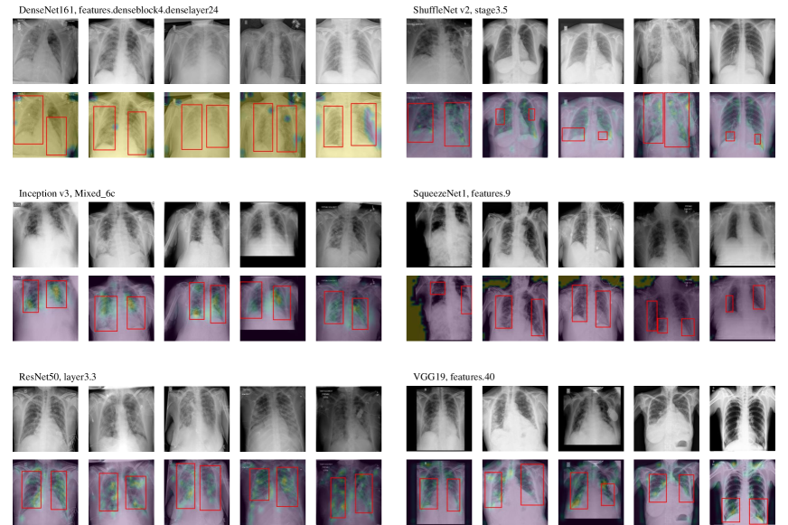
Figure S.3: Localization results of different models on the radiographs of COVID19 cases with typical symptoms. The red bounding boxes are the lesion regions drawn by doctors.

F.3 Visualizations of Localization Results on ImageNet, CUB-200-2011, and PASCAL VOC

ImageNet.

Figure S.22, S.23, S.24, S.25, and S.26 illustrate the localization results of applying whole classifier on images containing contents of whole, plant, animal, bird, and canine respectively. Figure S.27, S.28, and S.29 illustrate the localization results of applying mammal classifier on images containing contents of animal, mammal, and canine respectively. Note that some animals are not mammals and cannot be located. Figure S.26, S.29, and S.30 illustrate the localization results of applying whole, mammal, and carnivore classifiers on images containing contents of canine respectively.

CUB-200-2011.

Figure S.31, S.32, and S.33 illustrate the localization results of applying animal classifier trained on layer Mixed_6b of Inception v3, layer3.5 of ResNet50, and features.26 of VGG16 on the images from CUB-200-2011 respectively.

PASCAL VOC.

Figure S.34 shows the sample images from PASCAL VOC used for test with masks indicating the target objects. Figure S.35, S.36, and S.37 illustrate the localization results of applying whole, animal, and bird classifiers on the sample images. The classifiers are all trained on layer features.30 of VGG19 with 20 neurons selected by Shapley values. The results indicate the unique advantage of HINT for object localization: a flexible choice of localization targets.

Appendix G Ablation study

Illustration of the localization results of concept classifiers implemented with different saliency methods.

Figure S.38 shows the localization results of concept classifiers using Guided Backpropagation, Vanilla Backpropgation, Gradient x Input, Integrated Gradients, and SmoothGrad on dataset CUB-200-2011. The illustration indicates that HINT is general and can be implemented with different saliency methods.

Illustration of the localization results of concept classifiers trained with neurons chosen by shap, clf_coef, and random

Figure S.35, S.39, and S.40 show the localization results of applying whole classifiers on the sample images from PASCAL VOC, where the classifiers are trained on layer features.30 of VGG19 with 20 neurons selected by Shapley values (shap), selected by the coefficients of the linear classifier (clf_coef), and randomly selected (random) respectively. From observation, ”shap” locates more whole objects and larger object contents, indicating that Shapley values are good measures of neurons’ contributions to concepts.

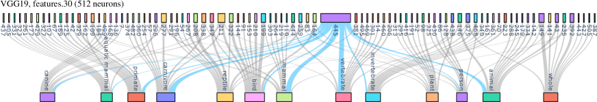
Figure S.4: Top-10 responsible neurons to concepts on layer “features.30” of VGG19.

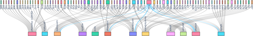
Figure S.5: Top-10 responsible neurons to concepts on layer “layer3.5” of ResNet50.

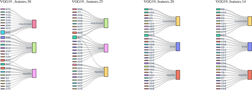
Figure S.6: Top-10 responsible neurons to concepts of mammal, bird, and reptile on different layer of VGG19.

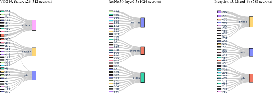
Figure S.7: Top-10 responsible neurons to concepts of animal, person, and plant of other models.

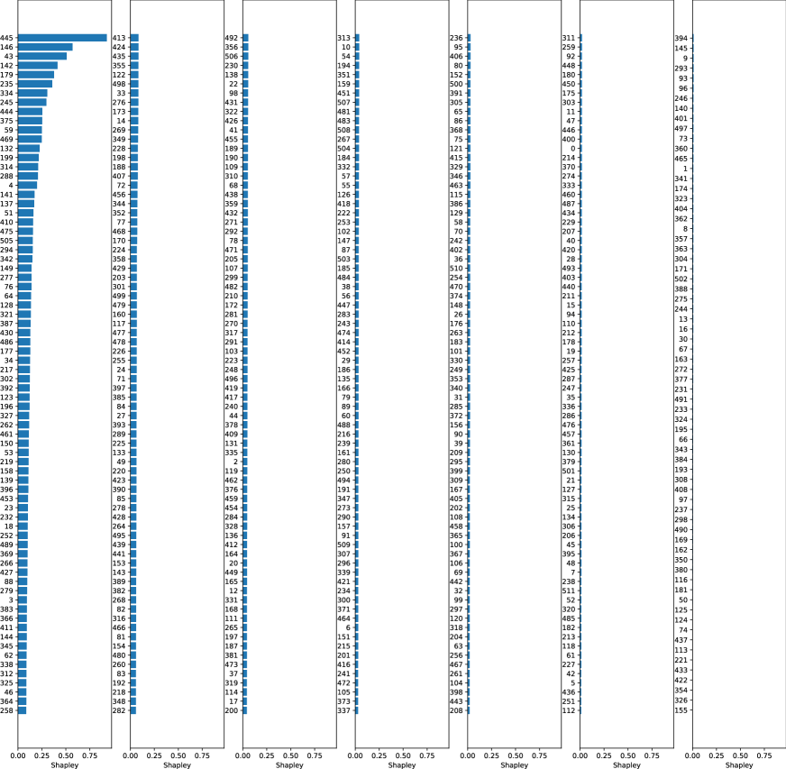
Figure S.8: Contribution scores (Shapley values) of neurons on layer features.30 of VGG19 to the concept of animal.

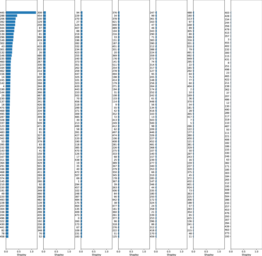
Figure S.9: Contribution scores (Shapley values) of neurons on layer features.30 of VGG19 to the concept of vertebrate.

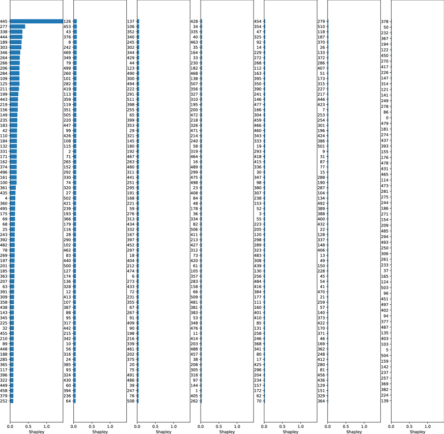
Figure S.10: Contribution scores (Shapley values) of neurons on layer features.30 of VGG19 to the concept of mammal.

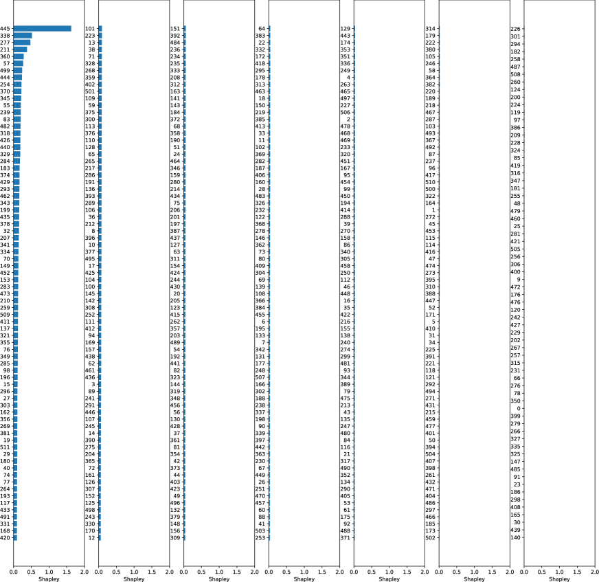
Figure S.11: Contribution scores (Shapley values) of neurons on layer features.30 of VGG19 to the concept of carnivore.

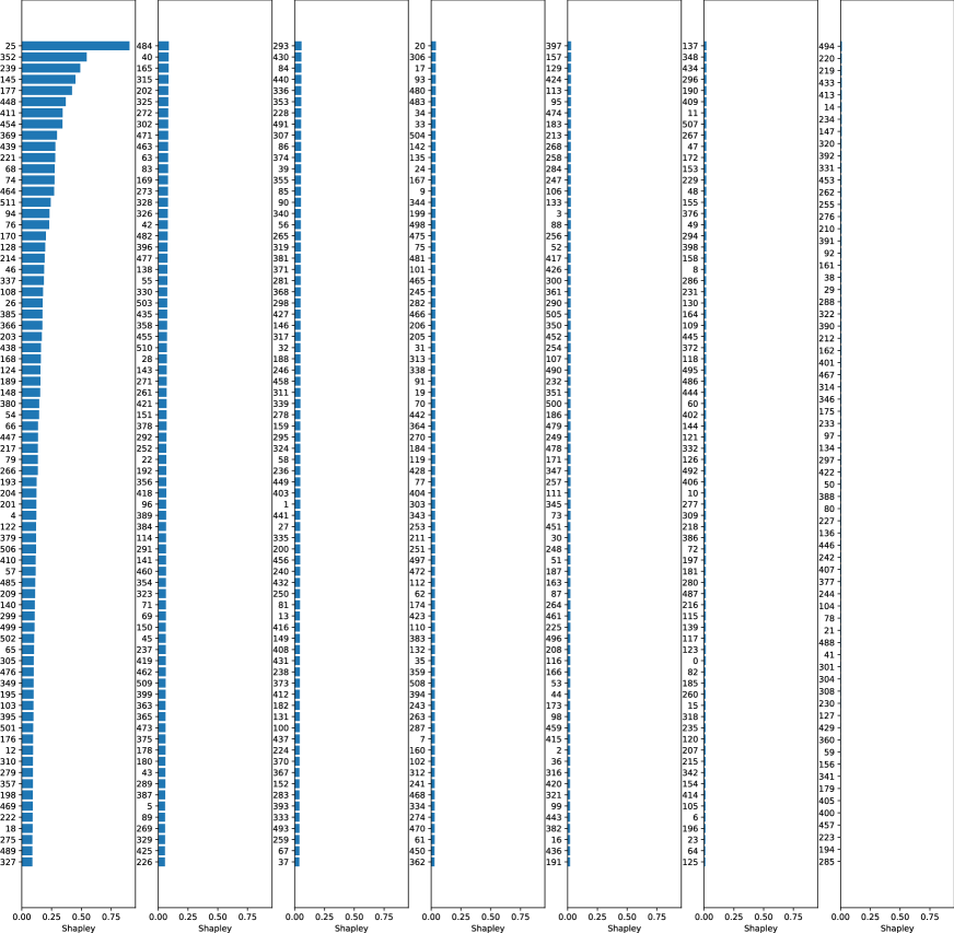
Figure S.12: Contribution scores (Shapley values) of neurons on layer features.26 of VGG16 to the concept of animal.

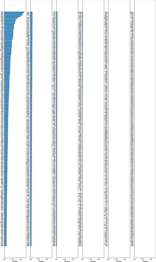
Figure S.13: Contribution scores (Shapley values) of neurons on layer layer3.5 of ResNet50 to the concept of animal.

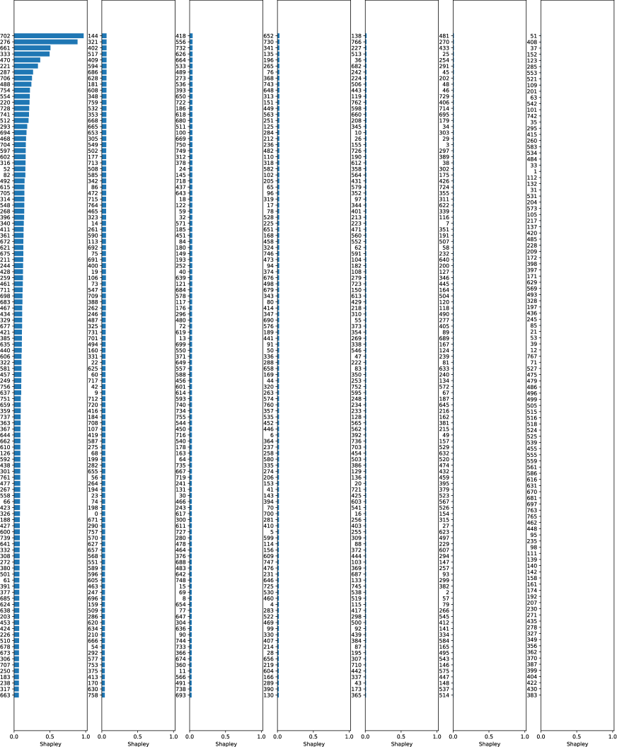
Figure S.14: Contribution scores (Shapley values) of neurons on layer Mixed_6b of Inception v3 to the concept of animal.

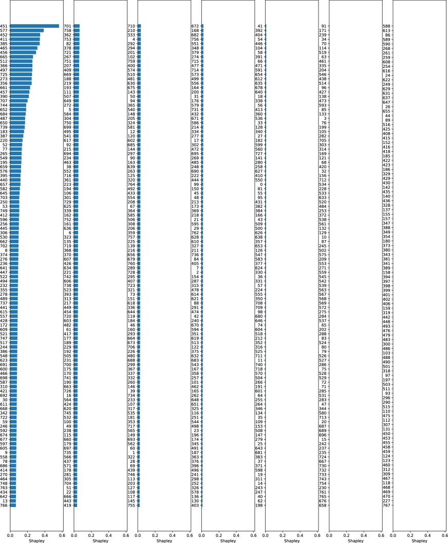
Figure S.15: Contribution scores (Shapley values) of neurons on layer Mixed_6b of Inception v3 to the concept of person.

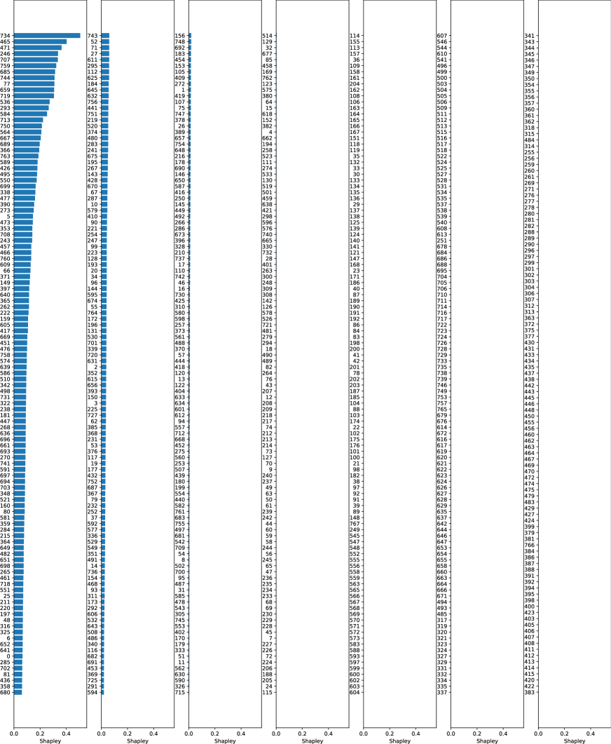
Figure S.16: Contribution scores (Shapley values) of neurons on layer Mixed_6b of Inception v3 to the concept of plant.

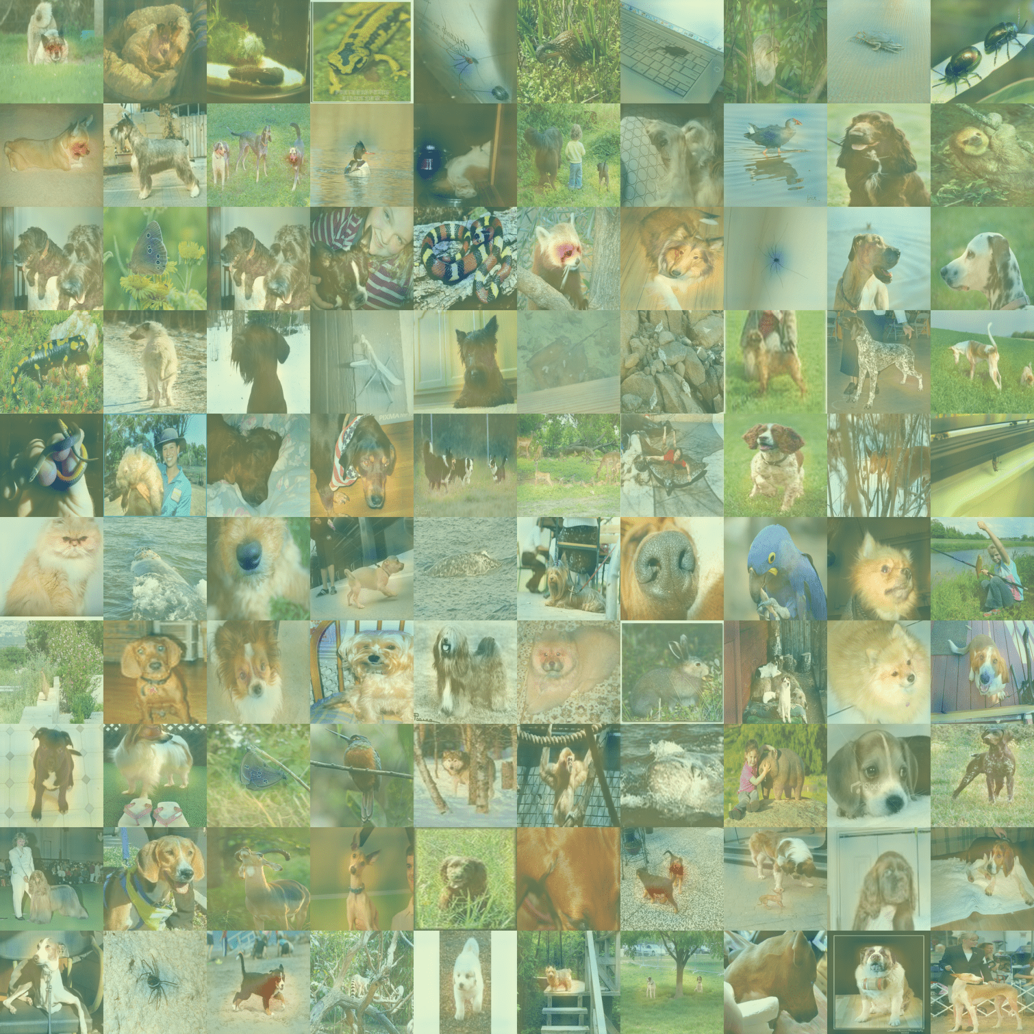
Figure S.17: Activation map of the $445^{th}$ neuron on animal images.

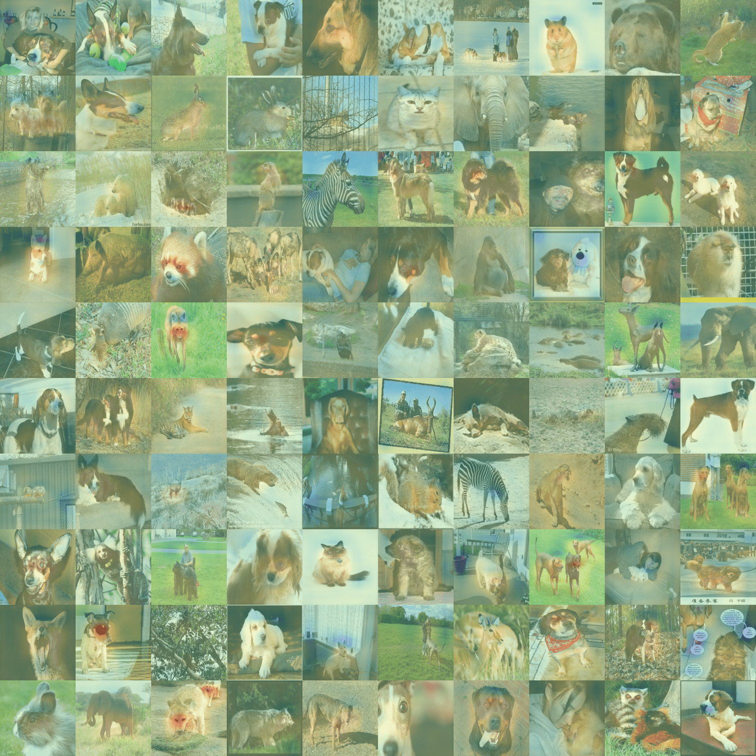
Figure S.18: Activation map of the $445^{th}$ neuron on mammal images.

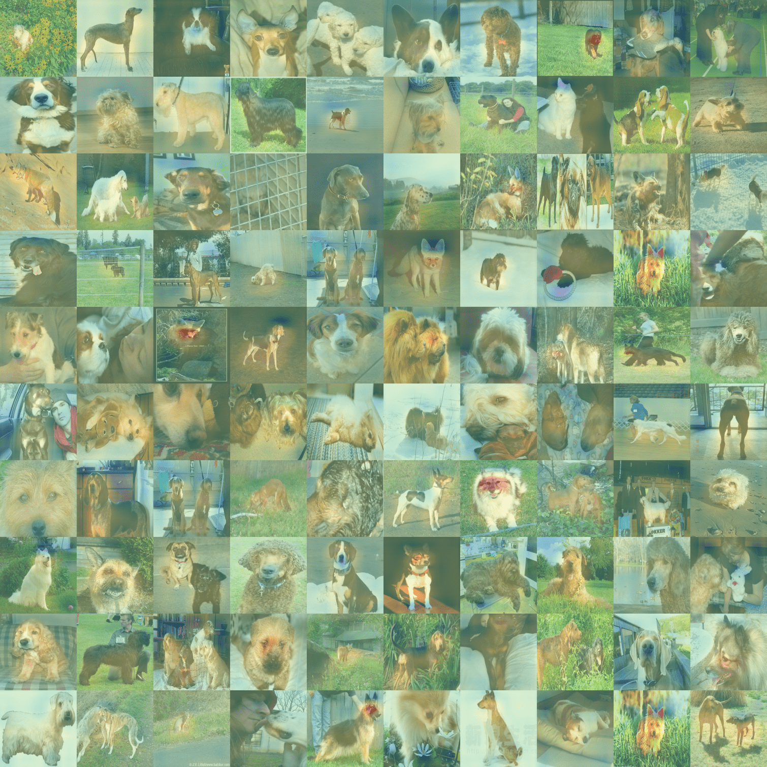
Figure S.19: Activation map of the $445^{th}$ neuron on canine images.

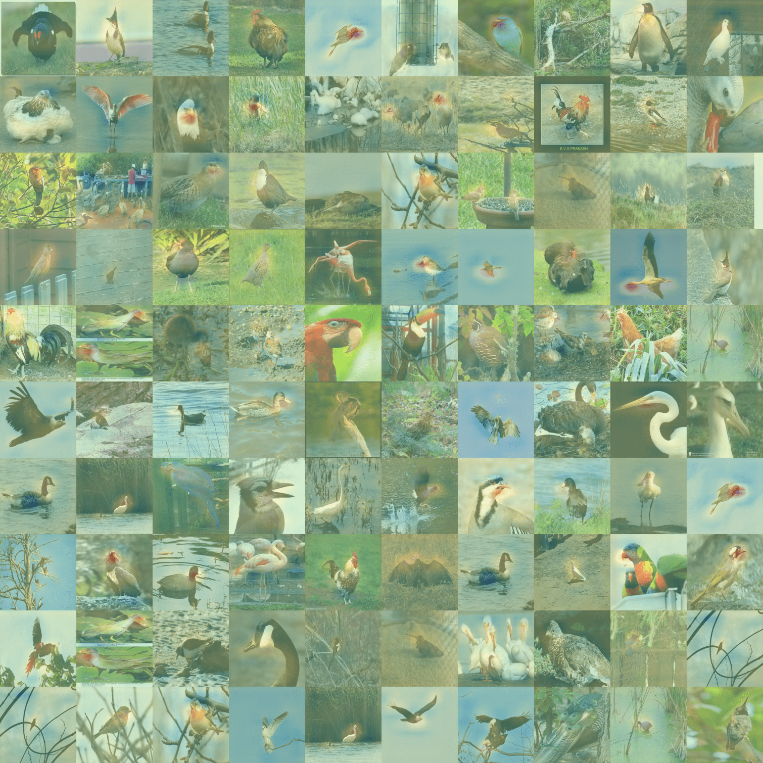
Figure S.20: Activation map of the $199^{th}$ neuron on bird images.

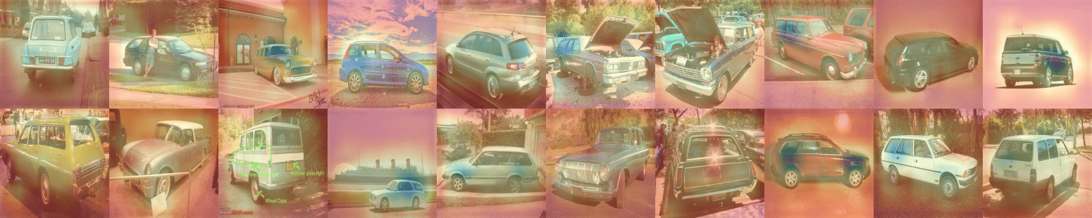
Figure S.21: Activation map of the $199^{th}$ neuron on car images.

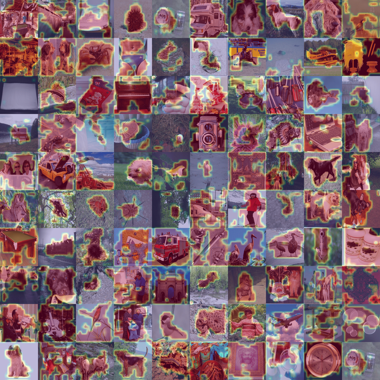
Figure S.22: Localization results of applying whole classifier on the images containing the concept of whole from ImageNet.

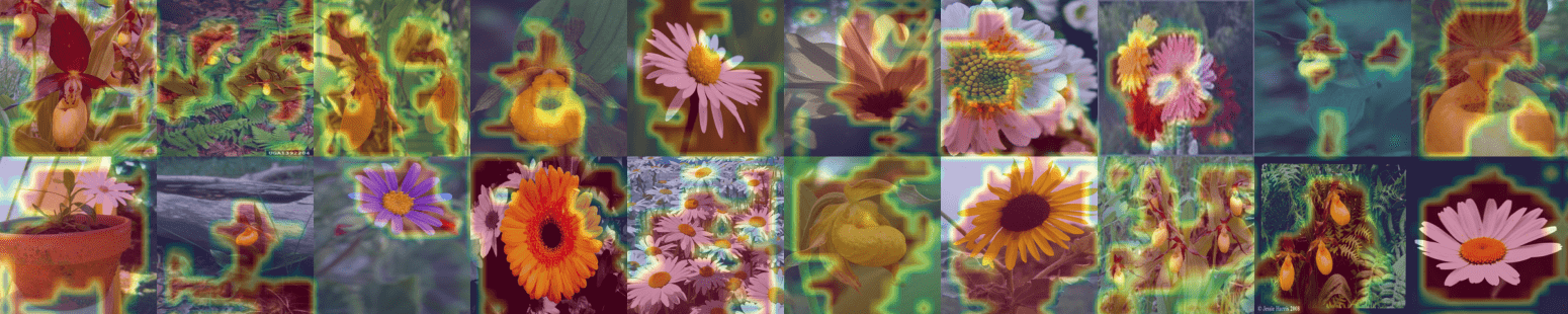
Figure S.23: Localization results of applying whole classifier on the images containing the concept of plant from ImageNet.

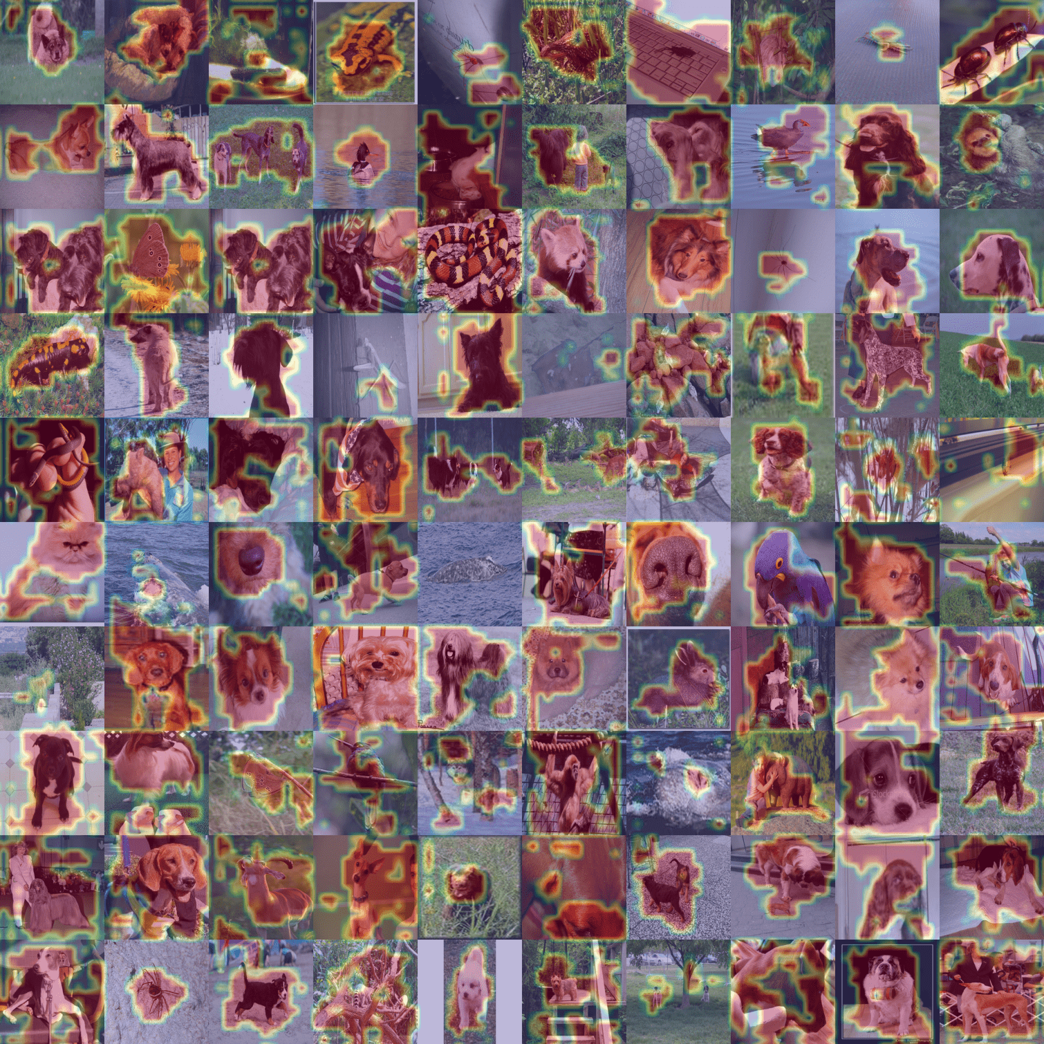
Figure S.24: Localization results of applying whole classifier on the images containing the concept of animal from ImageNet.

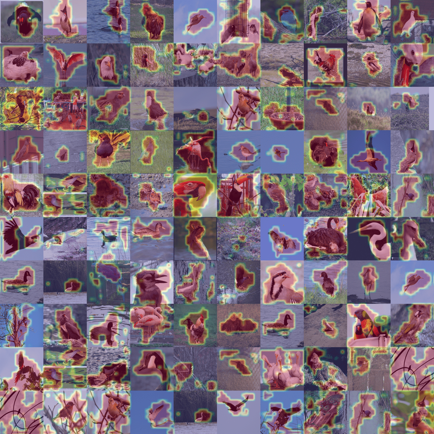
Figure S.25: Localization results of applying whole classifier on the images containing the concept of bird from ImageNet.

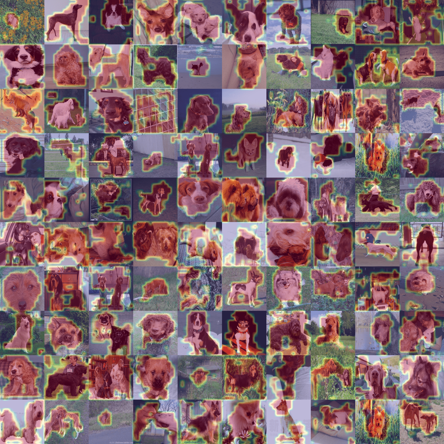
Figure S.26: Localization results of applying whole classifier on the images containing the concept of canine from ImageNet.

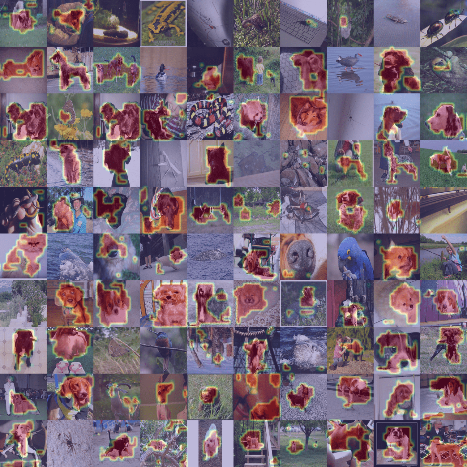
Figure S.27: Localization results of applying mammal classifier on the images containing the concept of animal from ImageNet. Note that some animals are not mammals and cannot be located.

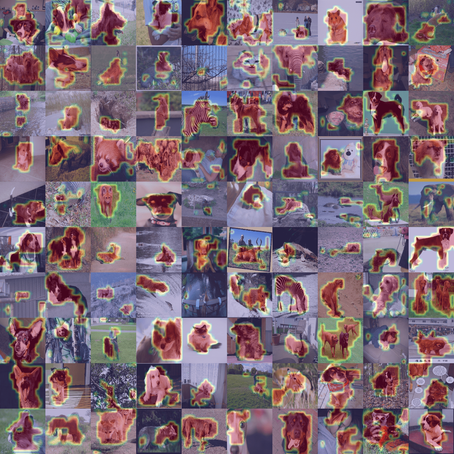
Figure S.28: Localization results of applying mammal classifier on the images containing the concept of mammal from ImageNet.

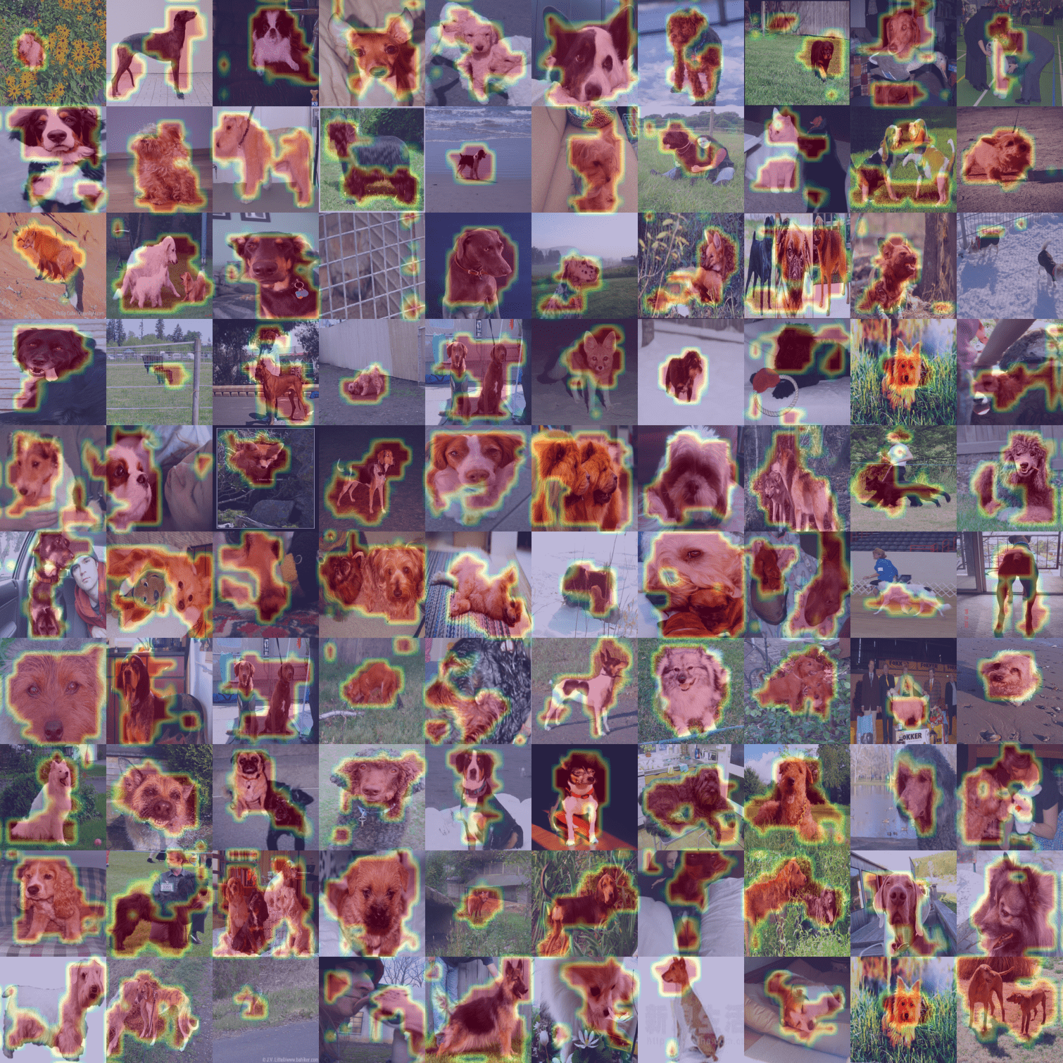
Figure S.29: Localization results of applying mammal classifier on the images containing the concept of canine from ImageNet.

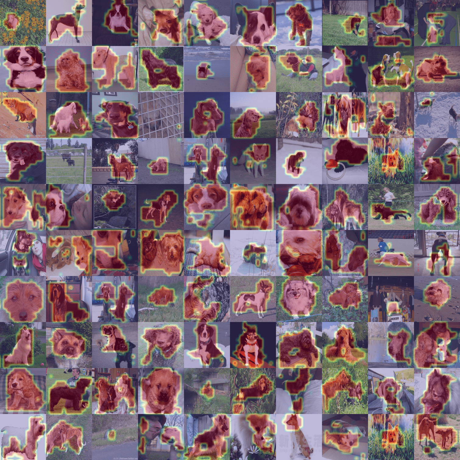
Figure S.30: Localization results of applying carnivore classifier on the images containing the concept of canine from ImageNet.

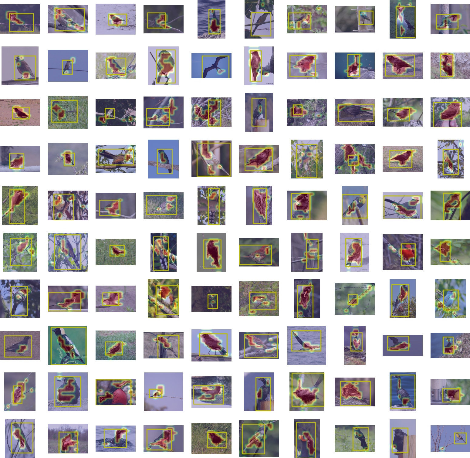
Figure S.31: Localization results of applying animal classifier trained on layer Mixed_6b of Inception v3 on the images from CUB-200-2011. The yellow bounding boxes are the groundtruth.

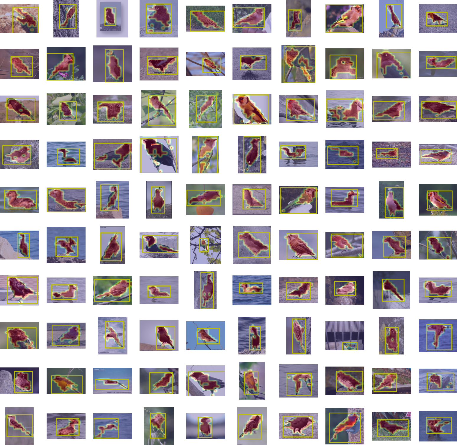
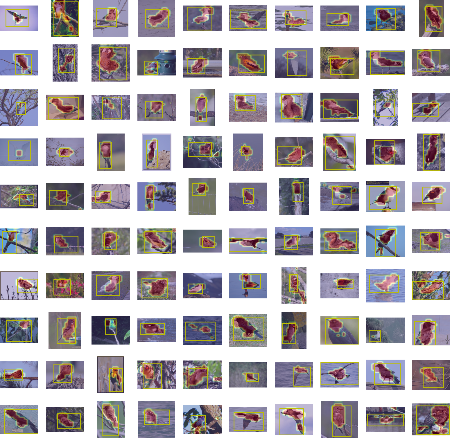
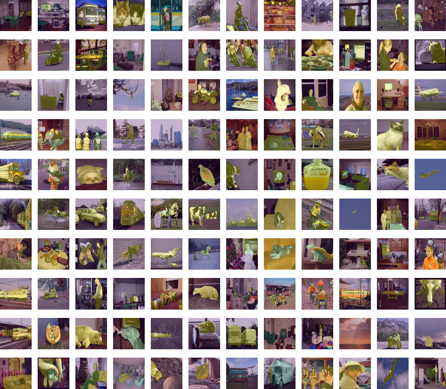
Figure S.32: Localization results of applying animal classifier trained on layer layer3.5 of ResNet50 on the images from CUB-200-2011. The yellow bounding boxes are the groundtruth.

Figure S.33: Localization results of applying animal classifier trained on layer features.26 of VGG16 on the images from CUB-200-2011. The yellow bounding boxes are the groundtruth.

Figure S.34: Sample images from PASCAL VOC with masks indicating the target objects.

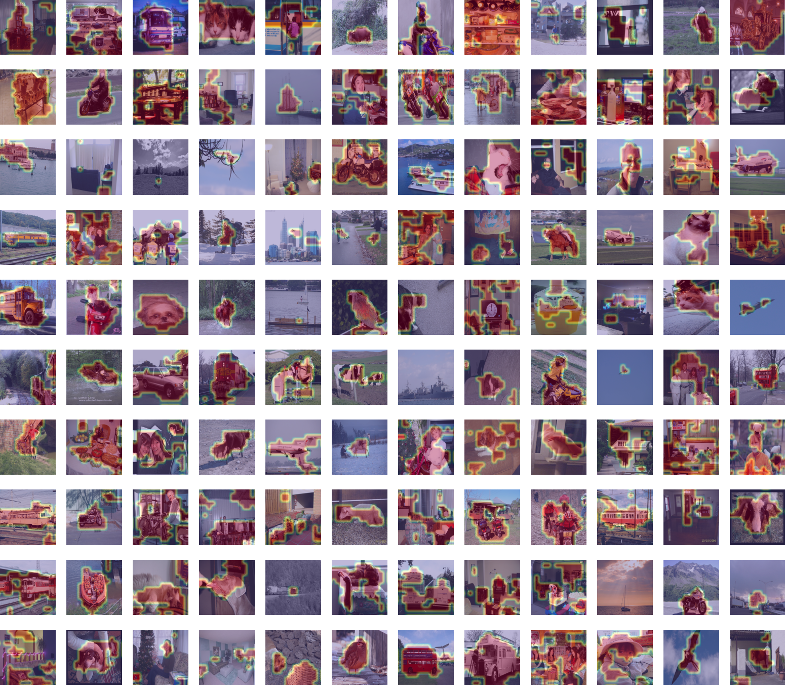
Figure S.35: Localization results of applying whole classifier on the sample images from PASCAL VOC. The classifier is trained on layer features.30 of VGG19 with 20 neurons selected by Shapley values.

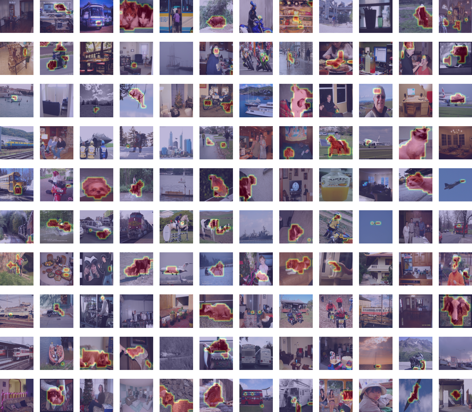
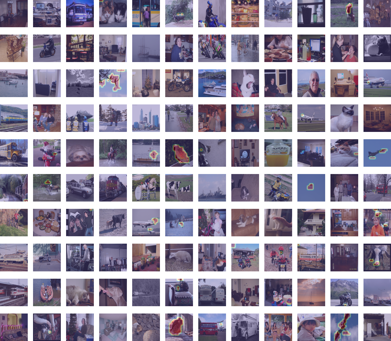
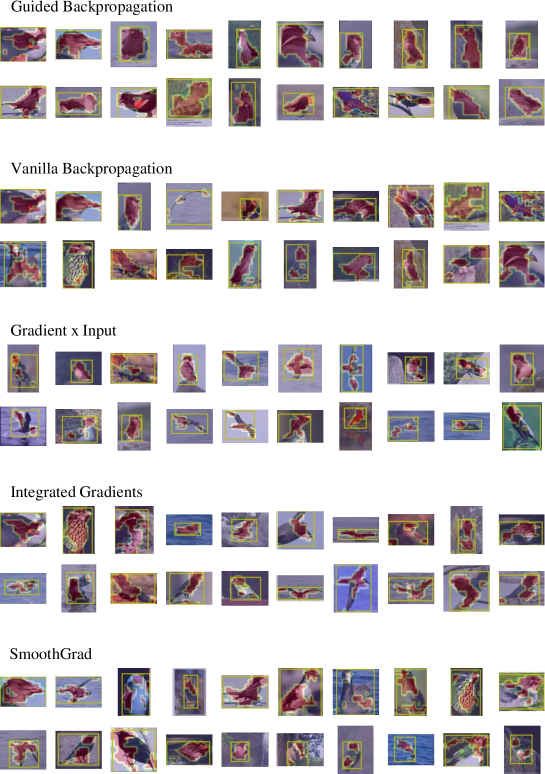
Figure S.36: Localization results of applying animal classifier on the sample images from PASCAL VOC. The classifier is trained on layer features.30 of VGG19 with 20 neurons selected by Shapley values.

Figure S.37: Localization results of applying bird classifier on the sample images from PASCAL VOC. The classifier is trained on layer features.30 of VGG19 with 20 neurons selected by Shapley values.

Figure S.38: Localization results of animal classifiers implemented with different modified saliency methods.

Figure S.39: Localization results of applying whole classifier on the sample images from PASCAL VOC. The classifier is trained on layer features.30 of VGG19 with 20 neurons selected by the coefficients of the linear classifier.

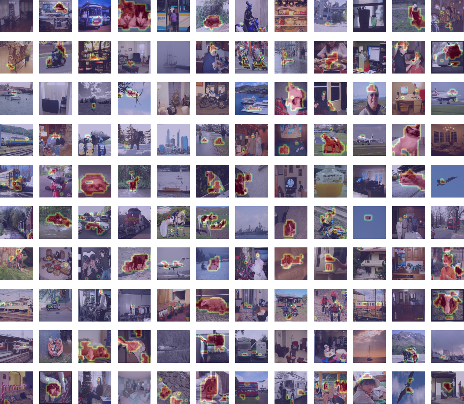
Figure S.40: Localization results of applying whole classifier on the sample images from PASCAL VOC. The classifier is trained on layer features.30 of VGG19 with 20 neurons randomly selected.

References

- [1] Julius Adebayo, Justin Gilmer, Michael Muelly, Ian Goodfellow, Moritz Hardt, and Been Kim. Sanity checks for saliency maps. arXiv preprint arXiv:1810.03292, 2018.
- [2] Sarah Adel Bargal, Andrea Zunino, Vitali Petsiuk, Jianming Zhang, Kate Saenko, Vittorio Murino, and Stan Sclaroff. Guided zoom: Questioning network evidence for fine-grained classification. In British Machine Vision Conference (BMVC), 2019.
- [3] Muhammad Aurangzeb Ahmad, Carly Eckert, and Ankur Teredesai. Interpretable machine learning in healthcare. In Proceedings of the 2018 ACM international conference on bioinformatics, computational biology, and health informatics, pages 559–560, 2018.
- [4] Anish Athalye, Logan Engstrom, Andrew Ilyas, and Kevin Kwok. Synthesizing robust adversarial examples. In International conference on machine learning, pages 284–293. PMLR, 2018.
- [5] Sebastian Bach, Alexander Binder, Grégoire Montavon, Frederick Klauschen, Klaus-Robert Müller, and Wojciech Samek. On pixel-wise explanations for non-linear classifier decisions by layer-wise relevance propagation. PloS one, 10(7):e0130140, 2015.
- [6] Wonho Bae, Junhyug Noh, and Gunhee Kim. Rethinking class activation mapping for weakly supervised object localization. In European Conference on Computer Vision, pages 618–634. Springer, 2020.
- [7] David Bau, Bolei Zhou, Aditya Khosla, Aude Oliva, and Antonio Torralba. Network dissection: Quantifying interpretability of deep visual representations. In Proceedings of the IEEE conference on computer vision and pattern recognition, pages 6541–6549, 2017.
- [8] David Bau, Jun-Yan Zhu, Hendrik Strobelt, Agata Lapedriza, Bolei Zhou, and Antonio Torralba. Understanding the role of individual units in a deep neural network. Proceedings of the National Academy of Sciences, 117(48):30071–30078, 2020.
- [9] David Bau, Jun-Yan Zhu, Hendrik Strobelt, Bolei Zhou, Joshua B Tenenbaum, William T Freeman, and Antonio Torralba. Gan dissection: Visualizing and understanding generative adversarial networks. arXiv preprint arXiv:1811.10597, 2018.
- [10] Tom B Brown, Dandelion Mané, Aurko Roy, Martín Abadi, and Justin Gilmer. Adversarial patch. arXiv preprint arXiv:1712.09665, 2017.
- [11] Shan Carter, Zan Armstrong, Ludwig Schubert, Ian Johnson, and Chris Olah. Exploring neural networks with activation atlases. Distill., 2019.
- [12] Chaofan Chen, Oscar Li, Daniel Tao, Alina Barnett, Cynthia Rudin, and Jonathan K Su. This looks like that: deep learning for interpretable image recognition. Advances in neural information processing systems, 32, 2019.
- [13] Hugh Chen, Scott Lundberg, and Su-In Lee. Explaining models by propagating shapley values of local components. In Explainable AI in Healthcare and Medicine, pages 261–270. Springer, 2021.
- [14] Junsuk Choe and Hyunjung Shim. Attention-based dropout layer for weakly supervised object localization. In Proceedings of the IEEE/CVF Conference on Computer Vision and Pattern Recognition, pages 2219–2228, 2019.
- [15] Piotr Dabkowski and Yarin Gal. Real time image saliency for black box classifiers. arXiv preprint arXiv:1705.07857, 2017.
- [16] Alex J DeGrave, Joseph D Janizek, and Su-In Lee. Ai for radiographic covid-19 detection selects shortcuts over signal. Nature Machine Intelligence, pages 1–10, 2021.
- [17] Jia Deng, Wei Dong, Richard Socher, Li-Jia Li, Kai Li, and Li Fei-Fei. Imagenet: A large-scale hierarchical image database. In 2009 IEEE conference on computer vision and pattern recognition, pages 248–255. Ieee, 2009.
- [18] M. Everingham, L. Van Gool, C. K. I. Williams, J. Winn, and A. Zisserman. The PASCAL Visual Object Classes Challenge 2007 (VOC2007) Results. http://www.pascal-network.org/challenges/VOC/voc2007/workshop/index.html.
- [19] Ruth Fong, Mandela Patrick, and Andrea Vedaldi. Understanding deep networks via extremal perturbations and smooth masks. In Proceedings of the IEEE/CVF International Conference on Computer Vision, pages 2950–2958, 2019.
- [20] Ruth Fong and Andrea Vedaldi. Net2vec: Quantifying and explaining how concepts are encoded by filters in deep neural networks. In Proceedings of the IEEE conference on computer vision and pattern recognition, pages 8730–8738, 2018.
- [21] Ruth C Fong and Andrea Vedaldi. Interpretable explanations of black boxes by meaningful perturbation. In Proceedings of the IEEE international conference on computer vision, pages 3429–3437, 2017.
- [22] Amirata Ghorbani, James Wexler, James Zou, and Been Kim. Towards automatic concept-based explanations. arXiv preprint arXiv:1902.03129, 2019.
- [23] Amirata Ghorbani and James Zou. Neuron shapley: Discovering the responsible neurons. arXiv preprint arXiv:2002.09815, 2020.
- [24] Mara Graziani, Vincent Andrearczyk, and Henning Müller. Regression concept vectors for bidirectional explanations in histopathology. In Understanding and Interpreting Machine Learning in Medical Image Computing Applications, pages 124–132. Springer, 2018.
- [25] Jindong Gu and Volker Tresp. Semantics for global and local interpretation of deep neural networks. arXiv preprint arXiv:1910.09085, 2019.
- [26] Jindong Gu, Yinchong Yang, and Volker Tresp. Understanding individual decisions of cnns via contrastive backpropagation. In Asian Conference on Computer Vision, pages 119–134. Springer, 2018.
- [27] Kaiming He, Xiangyu Zhang, Shaoqing Ren, and Jian Sun. Deep residual learning for image recognition. In Proceedings of the IEEE conference on computer vision and pattern recognition, pages 770–778, 2016.
- [28] Gao Huang, Zhuang Liu, Laurens Van Der Maaten, and Kilian Q Weinberger. Densely connected convolutional networks. In Proceedings of the IEEE conference on computer vision and pattern recognition, pages 4700–4708, 2017.
- [29] Forrest N Iandola, Song Han, Matthew W Moskewicz, Khalid Ashraf, William J Dally, and Kurt Keutzer. Squeezenet: Alexnet-level accuracy with 50x fewer parameters and¡ 0.5 mb model size. arXiv preprint arXiv:1602.07360, 2016.
- [30] Ashkan Khakzar, Sabrina Musatian, Jonas Buchberger, Icxel Valeriano Quiroz, Nikolaus Pinger, Soroosh Baselizadeh, Seong Tae Kim, and Nassir Navab. Towards semantic interpretation of thoracic disease and covid-19 diagnosis models. In International Conference on Medical Image Computing and Computer-Assisted Intervention, pages 499–508. Springer, 2021.
- [31] Been Kim, Rajiv Khanna, and Oluwasanmi O Koyejo. Examples are not enough, learn to criticize! criticism for interpretability. Advances in neural information processing systems, 29, 2016.
- [32] Been Kim, Martin Wattenberg, Justin Gilmer, Carrie Cai, James Wexler, Fernanda Viegas, et al. Interpretability beyond feature attribution: Quantitative testing with concept activation vectors (tcav). In International conference on machine learning, pages 2668–2677. PMLR, 2018.
- [33] Pieter-Jan Kindermans, Sara Hooker, Julius Adebayo, Maximilian Alber, Kristof T Schütt, Sven Dähne, Dumitru Erhan, and Been Kim. The (un) reliability of saliency methods. In Explainable AI: Interpreting, Explaining and Visualizing Deep Learning, pages 267–280. Springer, 2019.
- [34] Paras Lakhani, John Mongan, Chinmay Singhal, Quan Zhou, Katherine P Andriole, William F Auffermann, Prasanth Prasanna, Theresa Pham, Michael Peterson, Peter J Bergquist, et al. The 2021 siim-fisabio-rsna machine learning covid-19 challenge: Annotation and standard exam classification of covid-19 chest radiographs. OSF Preprints, 2021.
- [35] Zachary C Lipton. The mythos of model interpretability. int. conf. In Machine Learning: Workshop on Human Interpretability in Machine Learning, 2016.
- [36] Weizeng Lu, Xi Jia, Weicheng Xie, Linlin Shen, Yicong Zhou, and Jinming Duan. Geometry constrained weakly supervised object localization. In Computer Vision–ECCV 2020: 16th European Conference, Glasgow, UK, August 23–28, 2020, Proceedings, Part XXVI 16, pages 481–496. Springer, 2020.
- [37] Scott M Lundberg, Gabriel G Erion, and Su-In Lee. Consistent individualized feature attribution for tree ensembles. arXiv preprint arXiv:1802.03888, 2018.
- [38] Scott M Lundberg and Su-In Lee. A unified approach to interpreting model predictions. In Proceedings of the 31st international conference on neural information processing systems, pages 4768–4777, 2017.
- [39] Ningning Ma, Xiangyu Zhang, Hai-Tao Zheng, and Jian Sun. Shufflenet v2: Practical guidelines for efficient cnn architecture design. In Proceedings of the European conference on computer vision (ECCV), pages 116–131, 2018.
- [40] Aleksander Madry, Aleksandar Makelov, Ludwig Schmidt, Dimitris Tsipras, and Adrian Vladu. Towards deep learning models resistant to adversarial attacks. arXiv preprint arXiv:1706.06083, 2017.
- [41] Jinjie Mai, Meng Yang, and Wenfeng Luo. Erasing integrated learning: A simple yet effective approach for weakly supervised object localization. In Proceedings of the IEEE/CVF conference on computer vision and pattern recognition, pages 8766–8775, 2020.
- [42] James L McClelland and Timothy T Rogers. The parallel distributed processing approach to semantic cognition. Nature reviews neuroscience, 4(4):310–322, 2003.
- [43] Meng Meng, Tianzhu Zhang, Qi Tian, Yongdong Zhang, and Feng Wu. Foreground activation maps for weakly supervised object localization. In Proceedings of the IEEE/CVF International Conference on Computer Vision, pages 3385–3395, 2021.
- [44] George A Miller. Wordnet: a lexical database for english. Communications of the ACM, 38(11):39–41, 1995.
- [45] Christoph Molnar. Interpretable machine learning. Lulu. com, 2020.
- [46] Grégoire Montavon, Sebastian Lapuschkin, Alexander Binder, Wojciech Samek, and Klaus-Robert Müller. Explaining nonlinear classification decisions with deep taylor decomposition. Pattern Recognition, 65:211–222, 2017.
- [47] Alexander Mordvintsev, Christopher Olah, and Mike Tyka. Inceptionism: Going deeper into neural networks. Google AI Blog, 2015.
- [48] Jesse Mu and Jacob Andreas. Compositional explanations of neurons. Advances in Neural Information Processing Systems, 33:17153–17163, 2020.
- [49] Chris Olah, Alexander Mordvintsev, and Ludwig Schubert. Feature visualization: How neural networks build up their understanding of images. distill, 2018.
- [50] Chris Olah, Arvind Satyanarayan, Ian Johnson, Shan Carter, Ludwig Schubert, Katherine Ye, and Alexander Mordvintsev. The building blocks of interpretability. Distill, 3(3):e10, 2018.
- [51] Vitali Petsiuk, Abir Das, and Kate Saenko. Rise: Randomized input sampling for explanation of black-box models. arXiv preprint arXiv:1806.07421, 2018.
- [52] MR Quillian and Semantic Memory’in. Semantic information processing, ed. m. minsky, 1968.
- [53] Marco Tulio Ribeiro, Sameer Singh, and Carlos Guestrin. ” why should i trust you?” explaining the predictions of any classifier. In Proceedings of the 22nd ACM SIGKDD international conference on knowledge discovery and data mining, pages 1135–1144, 2016.
- [54] Lloyd S Shapley. 17. A value for n-person games. Princeton University Press, 2016.
- [55] Avanti Shrikumar, Peyton Greenside, and Anshul Kundaje. Learning important features through propagating activation differences. In International Conference on Machine Learning, pages 3145–3153. PMLR, 2017.
- [56] Avanti Shrikumar, Peyton Greenside, Anna Shcherbina, and Anshul Kundaje. Not just a black box: Learning important features through propagating activation differences. arXiv preprint arXiv:1605.01713, 2016.
- [57] Karen Simonyan, Andrea Vedaldi, and Andrew Zisserman. Deep inside convolutional networks: Visualising image classification models and saliency maps. arXiv preprint arXiv:1312.6034, 2013.
- [58] Karen Simonyan and Andrew Zisserman. Very deep convolutional networks for large-scale image recognition. arXiv preprint arXiv:1409.1556, 2014.
- [59] Daniel Smilkov, Nikhil Thorat, Been Kim, Fernanda Viégas, and Martin Wattenberg. Smoothgrad: removing noise by adding noise. arXiv preprint arXiv:1706.03825, 2017.
- [60] Jost Tobias Springenberg, Alexey Dosovitskiy, Thomas Brox, and Martin Riedmiller. Striving for simplicity: The all convolutional net. arXiv preprint arXiv:1412.6806, 2014.
- [61] Jiawei Su, Danilo Vasconcellos Vargas, and Kouichi Sakurai. One pixel attack for fooling deep neural networks. IEEE Transactions on Evolutionary Computation, 23(5):828–841, 2019.
- [62] Mukund Sundararajan, Ankur Taly, and Qiqi Yan. Axiomatic attribution for deep networks. In International Conference on Machine Learning, pages 3319–3328. PMLR, 2017.
- [63] Christian Szegedy, Vincent Vanhoucke, Sergey Ioffe, Jon Shlens, and Zbigniew Wojna. Rethinking the inception architecture for computer vision. In Proceedings of the IEEE conference on computer vision and pattern recognition, pages 2818–2826, 2016.
- [64] Mingxing Tan and Quoc Le. Efficientnet: Rethinking model scaling for convolutional neural networks. In International Conference on Machine Learning, pages 6105–6114. PMLR, 2019.
- [65] C. Wah, S. Branson, P. Welinder, P. Perona, and S. Belongie. The Caltech-UCSD Birds-200-2011 Dataset. Technical Report CNS-TR-2011-001, California Institute of Technology, 2011.
- [66] Zhou Wang and Alan C Bovik. Mean squared error: Love it or leave it? a new look at signal fidelity measures. IEEE signal processing magazine, 26(1):98–117, 2009.
- [67] Elizabeth K Warrington. The selective impairment of semantic memory. The Quarterly journal of experimental psychology, 27(4):635–657, 1975.
- [68] Daniel S Weld and Gagan Bansal. The challenge of crafting intelligible intelligence. Communications of the ACM, 62(6):70–79, 2019.
- [69] Haolan Xue, Chang Liu, Fang Wan, Jianbin Jiao, Xiangyang Ji, and Qixiang Ye. Danet: Divergent activation for weakly supervised object localization. In Proceedings of the IEEE/CVF International Conference on Computer Vision, pages 6589–6598, 2019.
- [70] Chih-Kuan Yeh, Cheng-Yu Hsieh, Arun Suggala, David I Inouye, and Pradeep K Ravikumar. On the (in) fidelity and sensitivity of explanations. Advances in Neural Information Processing Systems, 32:10967–10978, 2019.
- [71] Jason Yosinski, Jeff Clune, Anh Nguyen, Thomas Fuchs, and Hod Lipson. Understanding neural networks through deep visualization. arXiv preprint arXiv:1506.06579, 2015.
- [72] Matthew D Zeiler and Rob Fergus. Visualizing and understanding convolutional networks. In European conference on computer vision, pages 818–833. Springer, 2014.
- [73] Chen-Lin Zhang, Yun-Hao Cao, and Jianxin Wu. Rethinking the route towards weakly supervised object localization. In Proceedings of the IEEE/CVF Conference on Computer Vision and Pattern Recognition, pages 13460–13469, 2020.
- [74] Jianming Zhang, Sarah Adel Bargal, Zhe Lin, Jonathan Brandt, Xiaohui Shen, and Stan Sclaroff. Top-down neural attention by excitation backprop. International Journal of Computer Vision, 126(10):1084–1102, 2018.
- [75] Quanshi Zhang, Ruiming Cao, Feng Shi, Ying Nian Wu, and Song-Chun Zhu. Interpreting cnn knowledge via an explanatory graph. In Thirty-Second AAAI Conference on Artificial Intelligence, 2018.
- [76] Quanshi Zhang, Yu Yang, Haotian Ma, and Ying Nian Wu. Interpreting cnns via decision trees. In Proceedings of the IEEE/CVF Conference on Computer Vision and Pattern Recognition, pages 6261–6270, 2019.
- [77] Xiaolin Zhang, Yunchao Wei, Jiashi Feng, Yi Yang, and Thomas S Huang. Adversarial complementary learning for weakly supervised object localization. In Proceedings of the IEEE conference on computer vision and pattern recognition, pages 1325–1334, 2018.
- [78] Xiaolin Zhang, Yunchao Wei, Guoliang Kang, Yi Yang, and Thomas Huang. Self-produced guidance for weakly-supervised object localization. In Proceedings of the European conference on computer vision (ECCV), pages 597–613, 2018.
- [79] Bolei Zhou, David Bau, Aude Oliva, and Antonio Torralba. Interpreting deep visual representations via network dissection. IEEE transactions on pattern analysis and machine intelligence, 41(9):2131–2145, 2018.
- [80] Bolei Zhou, Aditya Khosla, Agata Lapedriza, Aude Oliva, and Antonio Torralba. Object detectors emerge in deep scene cnns. arXiv preprint arXiv:1412.6856, 2014.
- [81] Bolei Zhou, Aditya Khosla, Agata Lapedriza, Aude Oliva, and Antonio Torralba. Learning deep features for discriminative localization. In Proceedings of the IEEE conference on computer vision and pattern recognition, pages 2921–2929, 2016.