Laser-induced electron Fresnel diffraction by XUV pulses at extreme intensity

Abstract

Ionization of atoms and molecules in laser fields can lead to various interesting interference structures in the photoelectron spectrum. For the case of a super-intense extreme ultraviolet laser pulse, we identify a novel petal-like interference structure in the electron momentum distribution along the direction of the laser field propagation. We show that this structure is quite general and can be attributed to the Fresnel diffraction of the electronic wavepacket by the nucleus. Our results are demonstrated by numerically solving the time-dependent Schrödinger equation of the atomic hydrogen beyond the dipole approximation. By building an analytical model, we find that the electron displacement determines the aforementioned interference pattern. In addition, we establish the physical picture of laser-induced electron Fresnel diffraction which is reinforced by both quantum and semiclassical models.

As a fundamental law of quantum mechanics, the superposition of coherent electronic wavefunctions will result in interference. When exposed to external laser fields, the electrons in atoms and molecules can be ionized at different temporal and spatial positions Arbó et al. (2010); Xu et al. (2011); Waitz et al. (2016), which leads to various interference structures in the photoelectron spectrum. The dynamical and structural information Gopal et al. (2009); Korneev et al. (2012); Arbó et al. (2006a) is encoded in the spectrum through the phase of electronic wavefunction de Morisson Faria and Maxwell (2020). Experimentally, one can acquire the information about the targets by measuring the photoelectron momentum distribution (PMD) using the cold-target recoil-ion-momentum spectroscopy (COLTRIMS) Ullrich et al. (1997) or the velocity map imaging (VMI) spectrometers Chandler and Houston (1987); Eppink and Parker (1997). The theoretical analysis can be carried out by numerical solution of the time-dependent Schrödinger equation (TDSE) with high precision Huismans et al. (2011); Jiang et al. (2020), or by more intuitive semiclassical methods Li et al. (2014); Geng et al. (2015); Shvetsov-Shilovski et al. (2016) through the integration of the Newton equation of the electron, together with its classical phase de Morisson Faria and Maxwell (2020).

While the works mentioned above were carried out within the dipole approximation, strong-field physics beyond that approximation has attracted increasingly more interest in recent years Wang et al. (2020). It has been shown both experimentally and theoretically that nondipole corrections to the Hamiltonian can induce a photon-momentum transfer to the photoelectron Smeenk et al. (2011); Chelkowski et al. (2014); He et al. (2017); Wang et al. (2017); Liang et al. (2018); Chen et al. (2020); Ni et al. (2020). Besides, when atoms are exposed to the extreme ultraviolet (XUV) pulse of high intensity, the nondipole corrections can alter the dynamic interference Wang et al. (2018). With the further increase of the laser intensity, the nondipole effects become even more remarkable and the photoelectron angular distribution can be largely modified Førre et al. (2006) due to the strong interplay between the external electromagnetic and the internal Coulomb forces. The short-wavelength lasers at extreme intensities have been an everlasting pursuit Young and et al. (2018). In this regime, many new phenomena will be further identified.

In this Letter, we theoretically investigate the ionization dynamics of atoms exposed to a super-intense XUV laser pulse, based on the accurate numerical solution to TDSE beyond the dipole approximation. Our TDSE method is based on the finite element discrete variable representation Rescigno and McCurdy (2000) and the Arnoldi propagator Park and Light (1986). In the low-energy part of the PMD, we observe a novel petal-like interference structure along the direction of the pulse propagation. In this regime of laser parameters, the structure is quite robust and can be attributed to the Fresnel diffraction of the electronic wavepacket by the nucleus. Quantum and semiclassical models have been proposed to quantitatively reproduce the petal-like structures, which corroborate the physical mechanism of the laser-induced electron Fresnel diffraction.

Quantum-mechanical dynamics of an electron in a classical electromagnetic field is governed by the Schrödinger equation $i\partial_{t}\Psi({\mathbf{r}},t)=H\Psi({\mathbf{r}},t)$, in which the nondipole Hamiltonian $H$ in the propagation gauge and the long-wavelength approximation can be written as Førre and Simonsen (2016); Førre and Selstø (2020)

$$H =\frac{{\mathbf{p}}^{2}}{2}+{\mathbf{A}}(t)\cdot{\mathbf{p}}+V({\mathbf{r}})+\frac{{\mathbf{A}}^{2}(t)({\hat{\mathbf{k}}}\cdot{\mathbf{p}})}{2c}$$

$$+\frac{({\hat{\mathbf{k}}}\cdot{\mathbf{p}})({\mathbf{A}}(t)\cdot{\mathbf{p}})}{c}-\frac{({\hat{\mathbf{k}}}\cdot{\mathbf{r}})({\mathbf{\nabla}}V({\mathbf{r}})\cdot{\mathbf{A}}(t))}{c},$$ (1)

where all corrections of order $1/c$ beyond the dipole approximation have been included. (Atomic units are employed throughout the Letter unless otherwise stated, where $c\approx 137\,{\rm a.u.}$ is the speed of light.) Note that, in the dipole approximation, the Hamiltonian only contains the first three terms on the right hand side of Eq. (1).

In this Letter, we consider a linearly polarized laser pulse with the propagation vector $\hat{\mathbf{k}}$ in the $z$-direction. Its vector potential ${\mathbf{A}}(t)$ is given by

$${\mathbf{A}}(t)=\frac{\sqrt{I_{0}}}{\omega}\exp(-\frac{4\ln 2\,t^{2}}{\tau^{2}})\sin(\omega t){\hat{\mathbf{e}}_{x}},$$ (2)

where $I_{0}$ is the peak intensity, $\omega$ is the carrier frequency, and $\tau$ represents the full width at half maximum (FWHM). The corresponding electric field is ${\mathbf{E}}(t)=-\mathrm{d}{\mathbf{A}}(t)/\mathrm{d}t$.

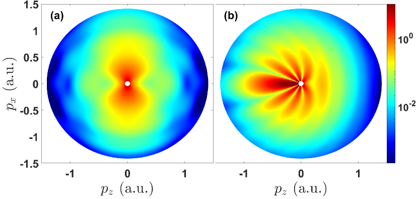
Figure 1: The PMDs in the $xz$-plane calculated either within (a) or beyond (b) the dipole approximation. See the main text for laser parameters.

Let us first examine the ionization of the ground state of the hydrogen atom by a laser pulse with $\omega=3\,{\rm a.u.}$, $\tau=2\sqrt{2}\pi\,{\rm a.u.}$, and $I_{0}=4\times 10^{20}\,{\rm W/{cm}^{2}}$. In Fig. 1, we show the PMDs within and beyond the dipole approximation. Only the low-energy parts below the one-photon ionization peak are demonstrated as the majority of the ionization occurs in this region. Although the spectra in both cases center around the zero momentum, they exhibit very distinct features. The PMD calculated within the dipole approximation is elongated in the $x$-direction. In the nondipole case, on the other hand, the PMD is most pronounced along the negative $z$-axis and is asymmetric about the $x$-axis. Compared to the simulations in Ref. Førre et al. (2006), novel petal-like interference lobes are present. We have numerically checked that the first nondipole term ${\mathbf{A}}^{2}(t)({\hat{\mathbf{k}}}\cdot{\mathbf{p}})/(2c)$ in Eq. (1), which originates from the radiation pressure Reiss (2014); Smeenk et al. (2011), is mainly responsible for the nondipole effects considered in our case. This term also indicates that a magnetic force ${\mathbf{F}}_{\rm m}=-{\rm A}(t){\rm E}(t)/c{\hat{\mathbf{e}}_{z}}$ is imposed on the electron Førre et al. (2006).

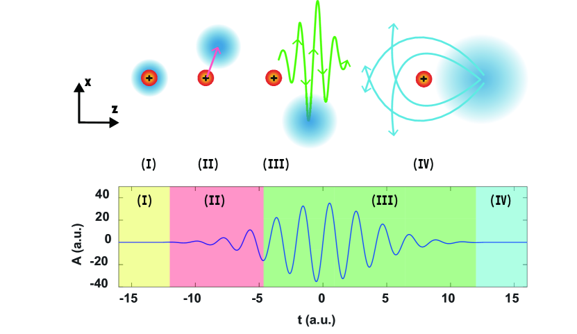
Figure 2: The cartoon representing the ionization process via four steps. The lines with arrows represent the trajectories of electrons. (I) The hydrogen atom is stationary without the laser field. (II) The electronic wave packet is non-adiabatically pulled away by the pulse in the rising portion of the envelope. (III) Next, it oscillates with the vector potential and moves forwards in the direction of pulse propagation. (IV) Finally, the electronic wave packet is diffracted by the nucleus. In addition, after step (II), the wave packet diffuses with time. Here, the nucleus is fixed at each step of the process whereas the vector potential as a function of time is plotted at the bottom.

In order to get more insight into the dynamics of photoelectrons, we present a movie in the Supplemental Materials mov , illustrating how the probability density distribution in the $xz$-plane varies in time. We note that the entire electronic wave packet is first pulled away from the nucleus. This is in contrast to the atomic stabilization in the Kramers-Henneberger frame Eberly and Kulander (1993), where the wave packet is split into two portions along the direction of field polarization and stays stable against ionization. This difference follows the fact that the adiabatic condition is not satisfied in our case Dörr and Potvliege (2000). After being pulled away, the electronic wave packet drifts in the laser field in the $\hat{\mathbf{k}}$ direction due to the magnetic force ${\mathbf{F}}_{\rm m}$. After the end of the laser pulse, the group velocity of the electronic wave packet is close to zero. Then, the diffusion of the wave packet induces spherical waves centered at a fixed position. The nucleus can be deemed as an obstruction for the induced spherical waves. One can compare this situation to the Fresnel diffraction in wave optics where the distance from the source to the obstruction is finite.

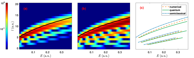
Figure 3: Color mappings of the energy-angular momentum distribution calculated from the TDSE (a) and quantum model (b), together with the relation (4) (black line). The comparison of the peak positions of these results is shown in (c), against the the semiclassical predictions (5) for $n=0,1,2$ from the top to the bottom, respectively.

The above mechanism can be depicted by a cartoon shown in Fig. 2. During the quiver motion of the electron, we have seen the isotropic diffusion of its wave packet mov , which indicates that the Coulomb force does not affect much the electron dynamics much when the intense laser field is present. Neglecting the Coulomb interaction, we obtain that the electron has a velocity component ${A^{2}}(t)/(2c){\hat{\mathbf{e}}_{z}}$, which is induced by the magnetic force. Hence, a classical electron displacement $z_{0}$ after the pulse (2) can be calculated,

$$z_{0}=\int_{-\infty}^{\infty}\frac{A^{2}(t)}{2c}dt\approx\sqrt{\frac{\pi}{2{\rm ln}2}}\,\frac{I_{0}\tau}{8\omega^{2}c}.$$ (3)

In wave optics, the distance from the source to the obstruction determines the Fresnel diffraction. Similarly, we shall show now that our diffraction patterns mainly depend on the classical displacement (3). This will be demonstrated analytically and confirmed numerically for various pulse durations and carrier frequencies.

According to Refs. Arbó et al. (2006b, 2008), the photoelectron angular distribution can be decomposed into contributing partial waves. Thus, one can examine the energy-angular momentum distributions of the ionized electrons. It was shown in Refs. Arbó et al. (2006b, 2008) that, for a low-energy electron ionized by an infrared laser, its angular momentum satisfies a classical relation $l=\sqrt{2\alpha+2\alpha^{2}E}$, where $E$ is the photoelectron energy and $\alpha$ is the amplitude of its quiver motion. For the low-energy spectrum in our case, we can carry out similar decompositions and the normalized $(E,l)$ joint distributions are presented in Fig. 3(a), in which the black line shows the special case of $\alpha=z_{0}$, i.e.,

$$l=\sqrt{2z_{0}+2z_{0}^{2}E}.$$ (4)

It is intriguing that the black line coincides with the main branch of the distribution though the electron is ionized by a very different pulse. Note that the classical angular momentum has been decreased by 0.5 for a better comparison with the TDSE results. Besides the main one, branches with smaller $l$ also appear in Fig. 3(a). They lead to the asymmetry of the PMDs about the $x$-axis. To further interpret our ab initio results in terms of the Fresnel diffraction, we recall that the electron dynamics can be described by a set of classical trajectories including phase in the semiclassical picture Li et al. (2014); Shvetsov-Shilovski et al. (2016). In our case, the induced spherical waves imply classical electrons with the same probability of emission in all directions. They are launched at $z_{0}$ when the pulse ends, which promises that there is more than one classical trajectory corresponding to each $(E,l)$ state, some of which have been intuitively depicted in Fig. 2 (IV). For a given angular momentum, there are two trajectories with the same energy that will contribute to interference (for electrons moving towards and away from the nucleus). The branches correspond to the interference enhancement of contributing orbits in the semiclassical picture. It can be shown that the $(E,l)$ relation is determined by sem

$$\int_{r_{\text{min}}}^{z_{0}}\sqrt{2(E-\frac{l^{2}}{2r^{2}}+\frac{1}{r})}dr=n\pi,$$ (5)

where $r_{\text{min}}={(\sqrt{1+2El^{2}}-1)}/{2E}$ and $n$ is a non-negative integer. These semiclassical results for $n=0,1,2$ are plotted in Fig. 3(c). The case for $n=0$ follows Eq. (4), which corresponds to the condition that the initial velocity of the electron is perpendicular to the $z$-axis in the semiclassical picture.

Our ab initio numerical results can also be understood based on a simplified quantum model. It is known that the radial part of the scattering state $R_{kl}(r)$ is analytically given in terms of the confluent hypergeometric function Landau and Lifshitz (2013). For the present case, the electronic wave function after the end of the pulse can be approximately written as $\delta(r-z_{0})\delta(\cos\theta-1)/r^{2}$, the $(E,l)$ distribution can then be shown to be

$$\left|a(E,l)\right|^{2}\propto\frac{2l+1}{\sqrt{E}}\left|R_{\sqrt{2E}l}(z_{0})\right|^{2}.$$ (6)

The results based on this formula are shown for comparison in Fig. 3(b), which reproduces the main interference features in Fig. 3(a). There do exist some differences, e.g., the simple quantum model overestimates the signals for smaller $l$ components. One also notes that the discrepancies become larger with the increase of $E$. They may be attributed to the finite volume of the electronic wave packet and to the effect of the Coulomb potential on the quiver motion of the electron.

For a better comparison, in Fig. 3(c), we draw the peak positions of results from the ab initio calculations and the quantum model against the prediction of the semiclassical model. Indeed, this comparison confirms that the numerically identified petal-like interference structures can be reproduced quantitatively by the simple quantum model and be understood qualitatively by the semiclassical one, which are based on the electron Fresnel diffraction by the nucleus.

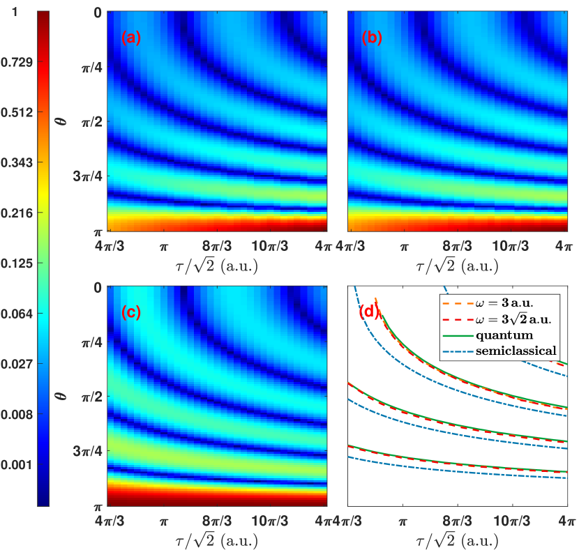
Figure 4: The normalized angular momentum distribution at $E_{s}=10^{-4}\,{\rm a.u.}$ for different FWHM $\tau$. The numerical color mappings are for $\omega=3\,{\rm a.u.}$ (a), $\omega=3\sqrt{2}\,{\rm a.u.}$ (b), and the analytical result (c) [Eq. (7)]. The comparison of the peak positions of different results is shown in (d).

As can be seen from Eqs. (5) and (6), the $(E,l)$ distributions of photoelectrons are determined by the classical displacement $z_{0}$. This in turn indicates that, in both semiclassical and quantum models, $z_{0}$ plays a major role in forming the diffraction patterns in PMDs. As it follows from the definition of the displacement $z_{0}$ [Eq. (3)], it changes with the peak intensity, the carrier frequency, and the duration of the laser pulse. To confirm the general validity of our models based on the Fresnel diffraction, numerical calculations of two other cases have been carried out. In the first case, the FWHM of the laser pulse $\tau$ varies from $4\sqrt{2}\pi/3\,{\rm a.u.}$ to $4\sqrt{2}\pi\,{\rm a.u.}$, whereas other parameters of the pulse are kept the same as before. In the second case, the duration $\tau$ is also gradually varied in the same interval, but the carrier frequency and the peak intensity of the pulse is changed to $\sqrt{2}\omega$ and $2I_{0}$ respectively. Note that, for both cases, the displacement $z_{0}$ is the same for a given $\tau$, which means that one should obtain the same PMDs. Without loss of generality for the discussion of the diffraction, one can consider the case of a small energy at $E_{s}=10^{-4}\,{\rm a.u.}$ In Figs. 4(a) and 4(b), we show the normalized photoelectron angular distributions at $E_{s}$ for the two cases respectively. First, we find that both color mappings are identical, which meets our expectations. In addition, we observe that the number of peaks in the angular distribution of photoelectrons increases for a longer pulse duration, which can be successfully accounted for by our semiclassical and quantum models. For the quantum model, when $E\rightarrow 0$, the scattering state of Coulomb potential becomes $R_{kl}/\sqrt{k}\,|_{\lim_{k\to 0}}=\sqrt{4\pi/r}J_{2l+1}(\sqrt{8r})$, where $J$ is the Bessel function Landau and Lifshitz (2013). Therefore, the angular distribution can be written as

$$\left|a(\theta,z_{0})\right|^{2}\propto\left|\sum_{l=0}^{l_{\max}}\frac{2l+1}{\sqrt{z_{0}}}J_{2l+1}(\sqrt{8z_{0}})P_{l}(\cos\theta)\right|^{2},$$ (7)

where $P_{l}$ is the Legendre polynomial and $l_{\max}$ is set to 25 in the present calculations. The normalized result according to Eq. (7) is presented in Fig. 4(c), which quantitatively reproduces the patterns shown in Figs. 4(a) and (b). Equivalently, the angular distribution patterns can also be qualitatively interpreted by our semiclassical model. For the zero-energy case, the semiclassical orbits become parabolas and thus the angular distribution can be described analytically as sem

$$\left|a(\theta,z_{0})\right|^{2}\propto\left|1+\exp[i4\sqrt{2z_{0}}\sin({\theta}/{2})]\right|^{2}.$$ (8)

It can be proven that the quantum model leads to the same PMDs as those of the semiclassical model when $z_{0}\to\infty$. For a better comparison, the peak positions of results from both TDSE and the quantum model are drawn against that of the semiclassical model, as shown in Fig. 4 (d). We can see that the ab initio results for the two cases almost coincide with the prediction of the quantum model, and the result of the semiclassical model qualitatively agrees with them.

Before concluding, we shall stress the differences of the diffraction discussed here from the laser-induced electron diffraction for molecules and rescattering for atoms, which are known in the literature Yurchenko et al. (2004); Meckel et al. (2008); Becker et al. (2018). For the latter two cases, recolliding electrons can be represented by plane waves with nonzero effective momenta. This can be interpreted as the Fraunhofer diffraction. In our case, however, the group velocity of the electron after it interacts with the pulse is zero, so the diffusion of the electron induces spherical waves centered at the distance $z_{0}$. These are the spherical waves rather than plane waves that diffract at the Coulomb potential. In other words, as already shown, we deal here with the Fresnel-type of diffraction. Though two types of diffraction are both induced by the combined action of the laser pulse and Coulomb force, the Fresnel-type diffraction induces more low-energy photoelectrons and is usually slower than the other one.

In conclusion, we have studied the dynamics of photoelectrons interacting with a super-intense XUV pulse. We found a novel petal-like diffraction structure along the laser pulse propagation direction in the low-energy part of the PMDs, which have been attributed to the laser-induced Fresnel diffraction of the electronic wave packet by the nucleus. Based on this diffraction picture, an intuitive semiclassical and a simplified quantum model have been developed and can analytically account for the novel interference patterns due to the nondipole effects. In addition, we show that this diffraction phenomenon is quite robust and general in the regime of super-intense XUV pulses.

This work is supported by the National Natural Science Foundation of China (NSFC) under Grant Nos. 11961131008 and 11725416, by the National Key R&D Program of China under Grant No. 2018YFA0306302, and by the National Science Centre (Poland) under Grant No. 2018/30/Q/ST2/00236.

References

- Arbó et al. (2010) D. G. Arbó, K. L. Ishikawa, K. Schiessl, E. Persson, and J. Burgdörfer, Phys. Rev. A 81, 021403(R) (2010).
- Xu et al. (2011) M.-H. Xu, L.-Y. Peng, Z. Zhang, and Q. Gong, J. Phys. B 44, 021001 (2011).
- Waitz et al. (2016) M. Waitz, D. Metz, J. Lower, C. Schober, M. Keiling, M. Pitzer, K. Mertens, M. Martins, J. Viefhaus, S. Klumpp, T. Weber, H. Schmidt-Böcking, L. P. H. Schmidt, F. Morales, S. Miyabe, T. N. Rescigno, C. W. McCurdy, F. Martín, J. B. Williams, M. S. Schöffler, T. Jahnke, and R. Dörner, Phys. Rev. Lett. 117, 083002 (2016).
- Gopal et al. (2009) R. Gopal, K. Simeonidis, R. Moshammer, T. Ergler, M. Dürr, M. Kurka, K.-U. Kühnel, S. Tschuch, C.-D. Schröter, D. Bauer, J. Ullrich, A. Rudenko, O. Herrwerth, T. Uphues, M. Schultze, E. Goulielmakis, M. Uiberacker, M. Lezius, and M. F. Kling, Phys. Rev. Lett. 103, 053001 (2009).
- Korneev et al. (2012) P. A. Korneev, S. V. Popruzhenko, S. P. Goreslavski, T.-M. Yan, D. Bauer, W. Becker, M. Kübel, M. F. Kling, C. Rödel, M. Wünsche, and G. G. Paulus, Phys. Rev. Lett. 108, 223601 (2012).
- Arbó et al. (2006a) D. G. Arbó, E. Persson, and J. Burgdörfer, Phys. Rev. A 74, 063407 (2006a).
- de Morisson Faria and Maxwell (2020) C. F. de Morisson Faria and A. S. Maxwell, Rep. Prog. Phys. 83, 034401 (2020).
- Ullrich et al. (1997) J. Ullrich, R. Moshammer, R. Dörner, O. Jagutzki, V. Mergel, H. Schmidt-Böcking, and L. Spielberger, J. Phys. B 30, 2917 (1997).
- Chandler and Houston (1987) D. W. Chandler and P. L. Houston, J. Chem. Phys. 87, 1445 (1987).
- Eppink and Parker (1997) A. T. J. B. Eppink and D. H. Parker, Rev. Sci. Instrum. 68, 3477 (1997).
- Huismans et al. (2011) Y. Huismans, A. Rouzée, A. Gijsbertsen, J. Jungmann, A. Smolkowska, P. Logman, F. Lepine, C. Cauchy, S. Zamith, T. Marchenko, et al., Science 331, 61 (2011).
- Jiang et al. (2020) W.-C. Jiang, S.-G. Chen, L.-Y. Peng, and J. Burgdörfer, Phys. Rev. Lett. 124, 043203 (2020).
- Li et al. (2014) M. Li, J.-W. Geng, H. Liu, Y. Deng, C. Wu, L.-Y. Peng, Q. Gong, and Y. Liu, Phys. Rev. Lett. 112, 113002 (2014).
- Geng et al. (2015) J.-W. Geng, W.-H. Xiong, X.-R. Xiao, L.-Y. Peng, and Q. Gong, Phys. Rev. Lett. 115, 193001 (2015).
- Shvetsov-Shilovski et al. (2016) N. I. Shvetsov-Shilovski, M. Lein, L. B. Madsen, E. Räsänen, C. Lemell, J. Burgdörfer, D. G. Arbó, and K. Tőkési, Phys. Rev. A 94, 013415 (2016).
- Wang et al. (2020) M.-X. Wang, S.-G. Chen, H. Liang, and L.-Y. Peng, Chin. Phys. B 29, 013302 (2020).
- Smeenk et al. (2011) C. T. L. Smeenk, L. Arissian, B. Zhou, A. Mysyrowicz, D. M. Villeneuve, A. Staudte, and P. B. Corkum, Phys. Rev. Lett. 106, 193002 (2011).
- Chelkowski et al. (2014) S. Chelkowski, A. D. Bandrauk, and P. B. Corkum, Phys. Rev. Lett. 113, 263005 (2014).
- He et al. (2017) P.-L. He, D. Lao, and F. He, Phys. Rev. Lett. 118, 163203 (2017).
- Wang et al. (2017) M.-X. Wang, X.-R. Xiao, H. Liang, S.-G. Chen, and L.-Y. Peng, Phys. Rev. A 96, 043414 (2017).
- Liang et al. (2018) H. Liang, M.-X. Wang, X.-R. Xiao, Q. Gong, and L.-Y. Peng, Phys. Rev. A 98, 063413 (2018).
- Chen et al. (2020) S.-G. Chen, W.-C. Jiang, S. Grundmann, F. Trinter, M. S. Schöffler, T. Jahnke, R. Dörner, H. Liang, M.-X. Wang, L.-Y. Peng, and Q. Gong, Phys. Rev. Lett. 124, 043201 (2020).
- Ni et al. (2020) H. Ni, S. Brennecke, X. Gao, P.-L. He, S. Donsa, I. Březinová, F. He, J. Wu, M. Lein, X.-M. Tong, and J. Burgdörfer, Phys. Rev. Lett. 125, 073202 (2020).
- Wang et al. (2018) M.-X. Wang, H. Liang, X.-R. Xiao, S.-G. Chen, W.-C. Jiang, and L.-Y. Peng, Phys. Rev. A 98, 023412 (2018).
- Førre et al. (2006) M. Førre, J. P. Hansen, L. Kocbach, S. Selstø, and L. B. Madsen, Phys. Rev. Lett. 97, 043601 (2006).
- Young and et al. (2018) L. Young and et al., J. Phys. B 51, 032003 (2018).
- Rescigno and McCurdy (2000) T. N. Rescigno and C. W. McCurdy, Phys. Rev. A 62, 032706 (2000).
- Park and Light (1986) T. J. Park and J. Light, J. Chem. Phys. 85, 5870 (1986).
- Førre and Simonsen (2016) M. Førre and A. S. Simonsen, Phys. Rev. A 93, 013423 (2016).
- Førre and Selstø (2020) M. Førre and S. Selstø, Phys. Rev. A 101, 063416 (2020).
- Reiss (2014) H. R. Reiss, J. Phys. B 47, 204006 (2014).
- (32) See Supplemental Material for the movie of the probability density varying with time .
- Eberly and Kulander (1993) J. Eberly and K. Kulander, Science 262, 1229 (1993).
- Dörr and Potvliege (2000) M. Dörr and R. Potvliege, J. Phys. B 33, L233 (2000).
- Arbó et al. (2006b) D. G. Arbó, S. Yoshida, E. Persson, K. I. Dimitriou, and J. Burgdörfer, Phys. Rev. Lett. 96, 143003 (2006b).
- Arbó et al. (2008) D. G. Arbó, K. I. Dimitriou, E. Persson, and J. Burgdörfer, Phys. Rev. A 78, 013406 (2008).
- (37) See Supplemental Material for details .
- Landau and Lifshitz (2013) L. D. Landau and E. M. Lifshitz, Quantum mechanics: non-relativistic theory, Vol. 3 (Elsevier, 2013).
- Yurchenko et al. (2004) S. N. Yurchenko, S. Patchkovskii, I. V. Litvinyuk, P. B. Corkum, and G. L. Yudin, Phys. Rev. Lett. 93, 223003 (2004).
- Meckel et al. (2008) M. Meckel, D. Comtois, D. Zeidler, A. Staudte, D. Pavičić, H. Bandulet, H. Pépin, J. Kieffer, R. Dörner, D. Villeneuve, et al., Science 320, 1478 (2008).
- Becker et al. (2018) W. Becker, S. Goreslavski, D. Milošević, and G. Paulus, J. Phys. B 51, 162002 (2018).
- Landau and Lifshitz (1976) L. D. Landau and E. M. Lifshitz, Mechanics: Volume 1 (Butterworth-Heinemann, 1976).
- Feynman et al. (2010) R. P. Feynman, A. R. Hibbs, and D. F. Styer, Quantum mechanics and path integrals (Courier Corporation, 2010).