RSTT: Real-time Spatial Temporal Transformer for Space-Time Video Super-Resolution

Abstract

Space-time video super-resolution (STVSR) is the task of interpolating videos with both Low Frame Rate (LFR) and Low Resolution (LR) to produce High-Frame-Rate (HFR) and also High-Resolution (HR) counterparts. The existing methods based on Convolutional Neural Network (CNN) succeed in achieving visually satisfied results while suffer from slow inference speed due to their heavy architectures. We propose to resolve this issue by using a spatial-temporal transformer that naturally incorporates the spatial and temporal super resolution modules into a single model. Unlike CNN-based methods, we do not explicitly use separated building blocks for temporal interpolations and spatial super-resolutions; instead, we only use a single end-to-end transformer architecture. Specifically, a reusable dictionary is built by encoders based on the input LFR and LR frames, which is then utilized in the decoder part to synthesize the HFR and HR frames. Compared with the state-of-the-art TMNet [54], our network is $60\%$ smaller (4.5M vs 12.3M parameters) and $80\%$ faster (26.2fps vs 14.3fps on $720\times 576$ frames) without sacrificing much performance. The source code is available at https://github.com/llmpass/RSTT.

1 Introduction

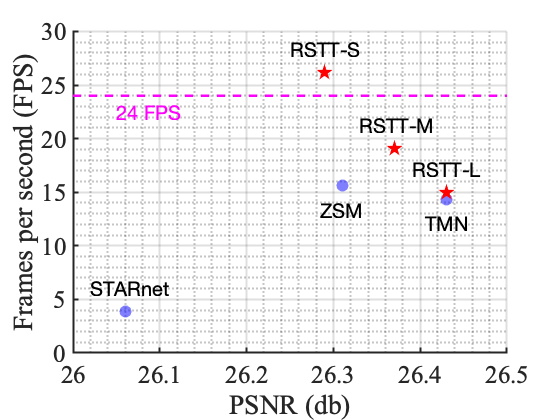
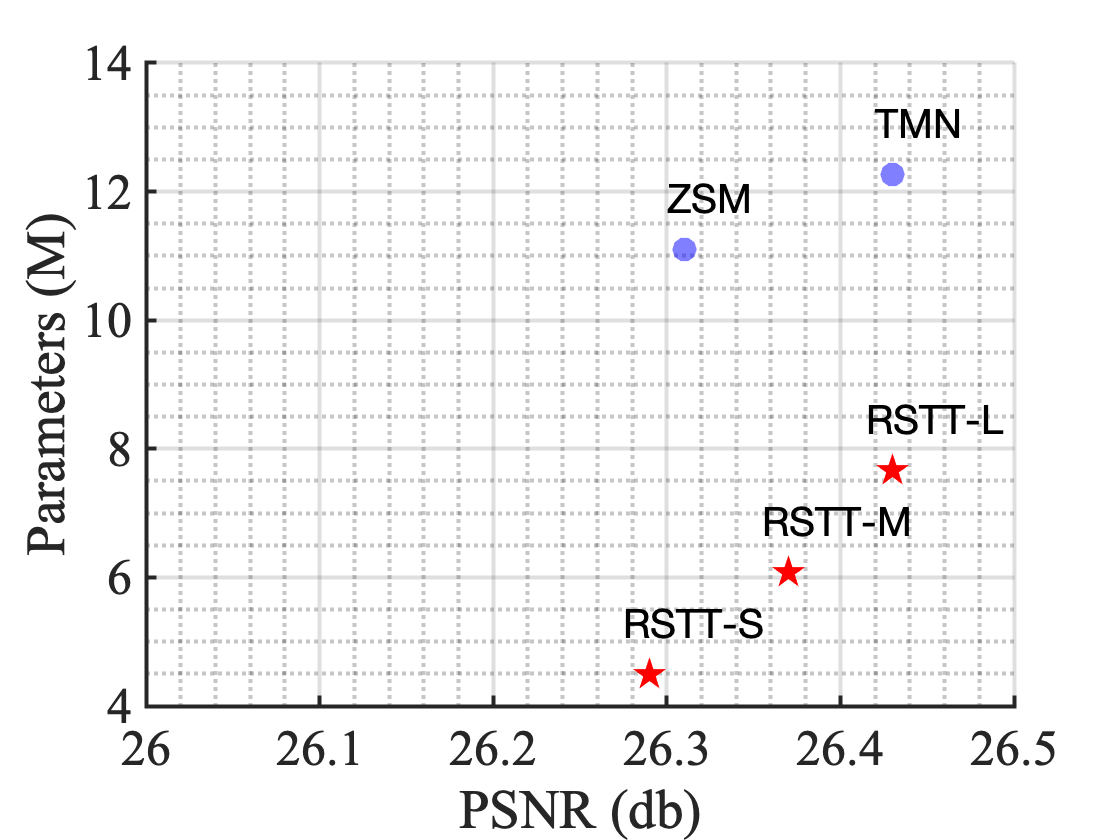
Figure 1: Performance of RSTT on Vid4 dataset [21] using small (S), medium (M) and large (L) architectures compared to other baseline models. In the top, we plot FPS versus PSNR. Note that 24 FPS is the standard cinematic frame rate [42]. In the bottom, we plot the number of parameters (in millions) versus PSNR. We omit the STARnet here since it is significantly larger than others while performs the worst; see Table 1 for details.

Space-time video super-resolution (STVSR) refers to the task of simultaneously increasing spatial and temporal resolutions of low-frame-rate (LFR) and low-resolution (LR) videos, which appears in a wide variety of multimedia applications such as video compression [36], video streaming [51], video conferencing [45] and so on. In the stage of deployment, many of them have stringent requirements for the computational efficiency, and only LFR and LR frames can be transferred in real-time. STVSR becomes a natural remedy in this scenario for recovering the high-frame-rate (HFR) and high-resolution (HR) videos. However, the performance of existing STVSR approaches are far from being real-time, and a fast method without sacrificing much visual quality is crucial for practical applications.

The success of traditional STVSR approaches usually relies on strong illumination consistency assumptions [29, 39], which can be easily violated in real world dynamic patterns. Ever since the era of deep neural network (DNN), convolutional neural network (CNN) exhibits promising results in many video restoration tasks, , video denoising [44, 8], video inpainting [18, 47], video super-resolution (VSR) [21, 17, 59, 49, 14] and video frame interpolation (VFI) [16, 1, 6, 33, 32, 30, 31, 11]. One straightforward way to tackle the STVSR problem is that by treating it as a composite task of VFI and VSR one can sequentially apply VFI, , SepConv [33], DAIN [1], CDFI [11], and VSR, , DUF [17], RBPN [14], EDVR [49], on the input LFR and LR video. Nevertheless, this simple strategy has two major drawbacks: first, it fails to utilize the inner connection between the temporal interpolation and spatial super-resolution [52, 54]; second, both VFI and VSR models need to extract and utilize features from nearby LR frames, which results in duplication of work. Additionally, such two-stage models usually suffer from slow inference speed due to the large amount of parameters, hence prohibits from being deployed on real-time applications.

To alleviate the above problems, recent learning based methods train a single end-to-end model [15, 52, 53, 54], where features are extracted from the input LFR and LR frames only once and then are upsampled in time and space sequentially inside the network. However, researches in this line still consist of two sub-modules: a temporal interpolation network, , Deformable ConvLSTM [52, 53] and Temporal Modulation Block [54], and a spatial reconstruction network, , residual blocks used in both Zooming SloMo [52, 53] and TMnet [54]. One natural question to ask is that whether we can have a holistic design such that it increases the spatial and temporal resolutions simultaneously without separating out the two tasks.

In this paper, we propose a single spatial temporal transformer that incorporates the temporal interpolation and spatial super resolution modules for the STVSR task. This approach leads to a much smaller network compared with the existing methods, and is able to achieve a real-time inference speed without sacrificing much performance. Specifically, we make the following contributions:

• We propose a Real-time Spatial Temporal Transformer (RSTT) to increase the spatial and temporal resolutions without explicitly modeling it as two sub-tasks. To the best of our knowledge, this is the first time that a transformer is utilized to solve the STVSR problem.

• Inside RSTT, we design a cascaded UNet-style architecture to effectively incorporate all the spatial and temporal information for synthesizing HFR and HR videos. In particular, the encoder part of RSTT builds dictionaries at multi-resolutions, which are then queried in the decoder part for directly reconstructing HFR and HR frames.

• We propose three RSTT models with different number of encoder and decoder pairs, resulting in small (S), medium (M) and larger (L) architectures. Experiments show that RSTT is significantly smaller and faster than the state-of-the-art STVSR methods while maintains similar performance: (i) RSTT-L performs similarly as TMNet [54] with $40\%$ less parameters, RSTT-M outperforms Zooming SlowMo [52] with $50\%$ less parameters and RSTT-S outperforms STARNet [15] with $96\%$ less parameters; (ii) RSTT-S achieves a frame rate of more than 24 per second (the standard cinematic frame rate) on $720\times 576$ frames. It achieves the performance of Zooming SlowMo [52] with a $75\%$ speedup, and outperforms STARNet [15] with around $700\%$ speedup (see Figure 1).

2 Related work

2.1 Video frame interpolation (VFI)

VFI aims at synthesizing an intermediate frame given two consecutive frames in a video sequence, hence the temporal resolution is increased. Conventionally, it is formulated as an image sequence estimation problem, , the path-based [26] and phase-based approach [27, 28], while it fails in scenes with fast movements or complex image details. CNN-based VFI methods can be roughly categorized into three types: flow-based, kernel-based and deformable-convolution-based. Flow-based methods [24, 16, 34, 57, 60, 30, 31] perform VFI by estimating optical flow between frames and then warping input frames with the estimated flow to synthesize the missing ones. Instead of using only pixel-wise information for interpolation, kernel-based methods [32, 33, 1, 2] propose to synthesize the image by convolving over local patches around each output pixel, which largely preserves the local textual details. Recently, deformable-convolution-based methods [19, 40, 7, 6, 11] combine flow-based and kernel-based methods by taking the advantages of flexible spatial sampling introduced by deformable convolution [9, 64]. This key improvement accommodates to both larger motions and complex textures.

2.2 Video super resolution (VSR)

VSR aims to recover HR video sequences from LR ones, hence the spatial resolution is increased. Most deep learning based VSR methods [22] adopt the strategy of fusing spatial features from multiple aligned frames (or features), which highly depends on the quality of the alignment. Earlier methods [4, 43, 37, 48, 57] utilize optical flow to perform explicit temporal frames alignment. However, the computation of optical flow can be expensive and the estimated flow can be inaccurate. In parallel, TDAN [59] introduces deformable convolution to implicitly align temporal features and achieves impressive performance, while EDVR [49] incorporates deformable convolution into a multi-scale module to further improve the feature alignments.

2.3 Space-time video super-resolution (STVSR)

The goal of STVSR is to increase both spatial and temporal resolutions of LFR and LR videos. Dating back two decades, [38] performs super-resolution simultaneously in time and space by modeling the dynamic scene as 3D representation. However, it requires input sequences of several different space-time resolutions to construct a new one. Due to the recent success of CNN, [15] proposes an end-to-end network STARnet to increase the spatial resolution and frame rate by jointly learning spatial and temporal contexts. Xiang et. al [52] propose a one-stage framework, named Zooming SlowMo, by firstly interpolating temporal features using deformable convolution and then fusing mutli-frame features through deformable ConvLSTM. Later, Xu et. al [54] incorporate temporal modulation block into Zooming SlowMo [52], named TMNet, so that the model is able to interpolate arbitrary intermediate frames and achieves better visual consistencies in between resulting frames. Nevertheless, these approaches either explicitly or implicitly treat the STVSR problem as a combination of VFI and VSR by designing separate modules for the sub-tasks, which is computationally expensive. Zhou et al. point out in a more recent work [63] that VFI and VSR mutually benefit each other. They present a network that cyclically uses the intermediate results generated by one task to improve another and vice versa. While achieving better performance, this idea results in a relatively larger network (about three times larger than Zooming SlowMo [52]). Our work also makes use of such mutual benefits from VFI and VSR, while avoids the repeated feature computations, and thus ends in a light-weight design.

2.4 Vision transformer

Transformer [46] is a dominant architecture in Natural Language Processing (NLP) and achieves state-of-the-art performance in various tasks [10, 3, 55]. Recently, transformers gain popularity in computer vision field. The pioneering Vision Transformer (ViT) [12] computes attentions between flattened image patches to solve image classification problems and outperforms CNN-based methods to a large extent. Due to transformer’s strong ability of learning long dependencies between different image regions, follow-up work using variants of ViT refreshes the state-of-the-art results in many applications, such as segmentation [41, 62], object detection [58, 56] and depth estimation [35]. In the meantime, Liu et al. [23] propose a novel transformer-based backbone for vision tasks, , Shifted window (Swin) Transformer, to reduce computational complexity by restricting the attention computations inside local and later shifted local windows. Thereafter, [50] proposes a U-shape network based on Swin Transformer for general image restoration. SwinIR [20] tackles the image restoration task using Swin Transformer and introduces residual Swin Transformer blocks. In this work, we also use Swin Transformer as basic building blocks to extract local information. However, instead of building dictionaries and queries from identical single frames [23, 5, 50, 20], we compute window and shifted window attentions from multiple input frames, which are then utilized to build reusable dictionaries to synthesize multiple output frames at once. We emphasize that this design is the key that leads to the acceleration of inference time and reduction of model size.

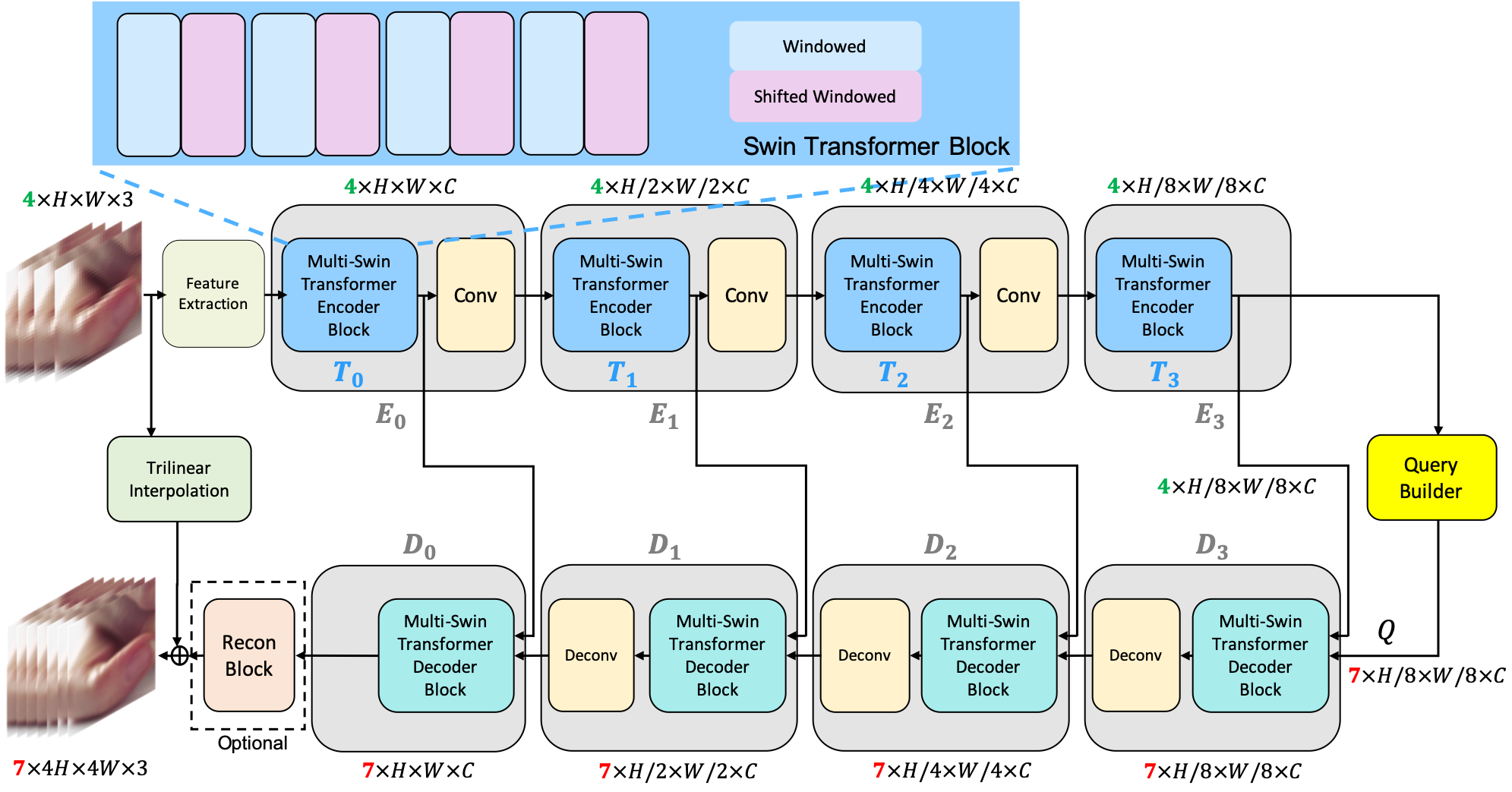
Figure 2: The architecture of the proposed RSTT. The features extracted from four input LFR and LR frames are processed by encoders $E_{k},k=0,1,2,3$ to build dictionaries that will be used as inputs for the decoders $D_{k},k=0,1,2,3$. The query builder generates a vector of queries ${Q}$ which are then used to synthesize a sequence of seven consecutive HFR and HR frames. The Multi-Swin transformer encoder and decoder blocks contain a set of repeated Swin Transformer Blocks, which are illustrated in more details in Figure 3 and 4.

3 The proposed method

In this section, we first give an overview of the proposed approach in Section 3.1. Then we explain the encoder and decoder part of our spatial-temporal transformer in Section 3.2 and Section 3.3, respectively. Finally, the training details are given in Section 3.4.

3.1 Network overview

Given $(n+1)$ LFR and LR frames $\mathcal{I}^{L}=\{I_{2t-1}^{L}\}_{t=1}^{n+1}$ of size $H\times W\times 3$, a STVSR model generates $2n+1$ HFR and HR frames $\mathcal{I}^{H}=\{I_{t}^{H}\}_{t=1}^{2n+1}$ of size $4H\times 4W\times 3$, where $t$ denotes the time stamp of a frame. Note that only frames with odd time stamp in $\mathcal{I}^{H}$ has the LR counterparts in $\mathcal{I}^{L}$.

We propose a cascaded UNet-style transformer, named Real-time Spatial Temporal Transformer (RSTT), to interpolate the LR sequence $\mathcal{I}^{L}$ in both time and space simultaneously without having explicit separations of the model into spatial and temporal interpolation modules. One may shortly observe that this design is a distinct advantage over the existing CNN-based methods since it leads to a real-time inference speed while maintains similar performance.

We let $f$ denote the underlying function modeled by RSTT, which takes four consecutive LFR and LR frames in $\mathcal{I}^{L}$ and outputs seven HFR and HR frames in the sequence:

$$\begin{split}f&:(I_{2t-1}^{L},I_{2t+1}^{L},I_{2t+3}^{L},I_{2t+5}^{L})\\ &\mapsto(I_{2t-1}^{H},I_{2t}^{H},I_{2t+1}^{H},I_{2t+2}^{H},I_{2t+3}^{H},I_{2t+4}^{H},I_{2t+5}^{H})\end{split}$$ (1)

As illustrated in Figure 2, RSTT mainly consists of four encoders $E_{k},k=0,1,2,3$, and corresponding decoders $D_{k},k=0,1,2,3$. In RSTT, a feature extraction block firstly extracts the features of the four input frames, denoted by $(F_{2t-1}^{L},F_{2t+1}^{L},F_{2t+3}^{L},F_{2t+5}^{L})$; then, a multi-video Swin Transformer encoder block $\mathcal{T}_{\text{swin}}$ takes the features as input:

$$T_{0}=\mathcal{T}_{\text{swin}}(F_{2t-1}^{L},F_{2t+1}^{L},F_{2t+3}^{L},F_{2t+5}^{L}),$$

where $T_{0}$ is the embedded feature generated by Swin Transformer. Let $\Phi$ denote the convolutional block in $E_{0},E_{1}$ and $E_{2}$, one can write $E_{0}=\Phi(T_{0})$. Subsequently, we have

$$\begin{cases}T_{k}=\mathcal{T}_{\text{swin}}(E_{k-1}),&\quad k=1,2,3\\ E_{k}=\Phi(T_{k}),&\quad k=1,2\\ E_{3}=T_{3}\end{cases}$$ (2)

Note that each of the encoders $E_{k},k=0,1,2,3$, has four output channels corresponding to the four time stamps of the input LFR and LR frames. To make it clear, we use

$$E_{k}\equiv(E_{k,2t-1},E_{k,2t+1},E_{k,2t+3},E_{k,2t+5})$$

to denote the four output feature maps of each $E_{k}$. In fact, a reusable dictionary is built in each $E_{k}$, and the details of the encoder architecture are presented in Section 3.2.

After computing $E_{3}$, RSTT constructs a query builder that generates features for interpolating HFR and HR frames at finer time stamps. Specifically, we define the query $Q$ as seven-channel feature maps with

$$\begin{split}Q:=\Big{(}E_{3,2t-1},&\tfrac{1}{2}(E_{3,2t-1}+E_{3,2t+1}),E_{3,2t+1},\\ &\tfrac{1}{2}(E_{3,2t+1}+E_{3,2t+3}),E_{3,2t+3},\\ &\tfrac{1}{2}(E_{3,2t+3}+E_{3,2t+5}),E_{3,2t+5}\Big{)}\end{split}$$ (3)

As indicated in (3), for odd HFR and HR frames which already have their LFR and LR counterparts, we just adopt the learnt features from the encoder $E_{3}$ as the queries; while for even frames that have no LFR and LR counterparts, we use the mean features of their adjacent frames as the queries.

We are now ready to synthesize the HFR and HR frames by feeding the decoders with the query and the outputs of encoders. As shown in Figure 2, similar to (2), we have

$$\begin{cases}D_{3}=\Phi^{-1}(\mathcal{T}^{-1}_{\text{swin}}(T_{3},Q)),\\ D_{k}=\Phi^{-1}(\mathcal{T}^{-1}_{\text{swin}}(T_{k},D_{k+1})),&\quad k=1,2\\ D_{0}=\mathcal{T}^{-1}_{\text{swin}}(T_{0},D_{1})\end{cases}$$ (4)

where $\mathcal{T}^{-1}_{\text{swin}}$ is the multi-video Swin Transformer decoder block and $\Phi^{-1}$ denotes the deconvolutional block in $D_{1},D_{2}$ and $D_{3}$. The details of the decoder architecture are presented in Section 3.3. For the final synthesis, we learn the residuals instead of the HFR and HR frames themselves. We simply use a trilinear interpolation of the input frames to work as a warming start of the output frames.

We remark that the key to the architecture of RSTT is the reusable dictionaries built in the encoders $E_{k}$ based on the input LFR and LR frames, which are then utilized in decoders ${D}_{k}$ combined with queries to synthesize the HFR and HR frames. This design is advantageous over the duplicate feature fusions appearing in many existing methods, , deformable convolutions and ConvLSTM in Zooming SlowMo [52] and TMNet [54]), and thus accelerates the inference speed to a large extent.

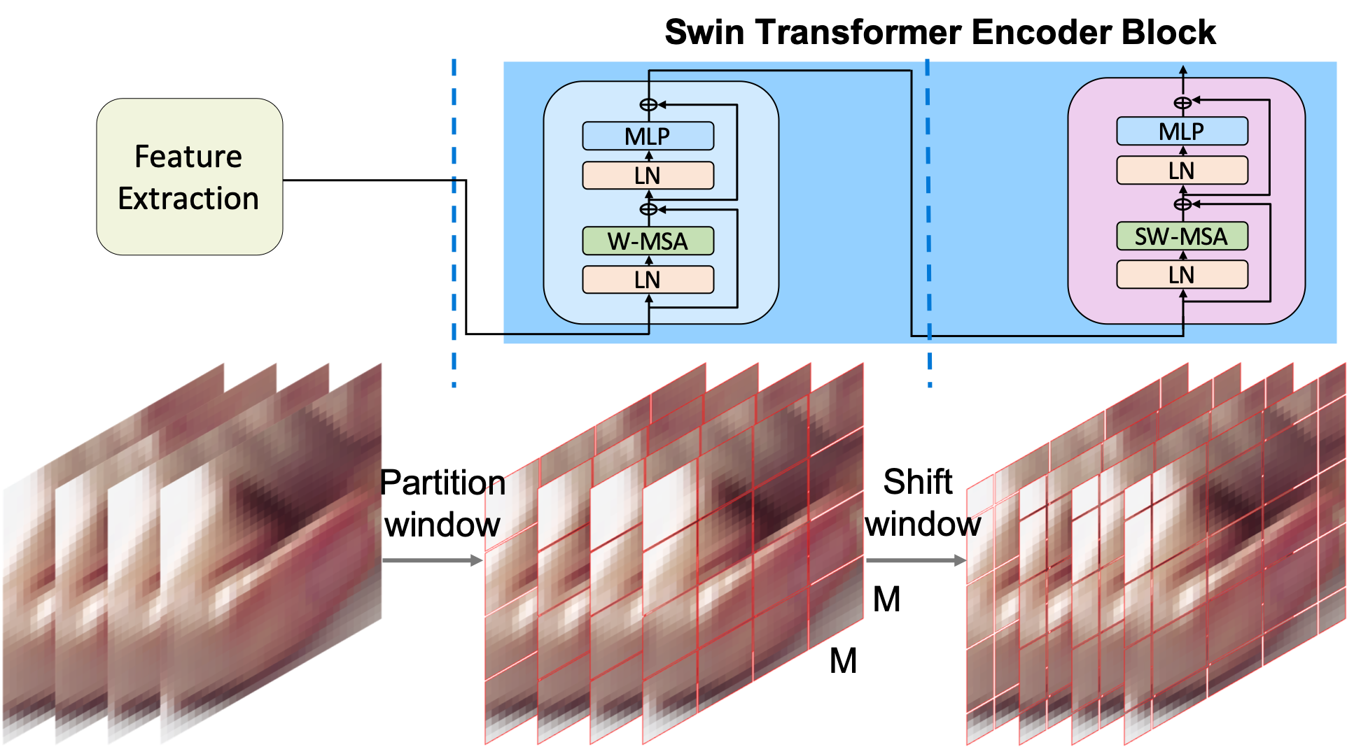
Figure 3: The basic Swin Transformer encoder block used in $\bm{E_{k},k=0,1,2,3}$ of RSTT; see Figure 2. It first computes multi-head self attentions in each window partition, and then in each shifted window partition. Here, LN stands for Layer Normalization, W-MSA is Windowed Multi-Head Self-Attention and SW-MSA is Shifted Windowed Multi-Head Self-Attention.

3.2 Encoder

In this subsection, we explain in details the encoder architecture of our RSTT. Before moving on, for the feature extraction module shown in Figure 2, we use a single convolutional layer with kernel size $3\times 3$ to extract $C$ features from four input LFR and LR RGB frames. This shallow feature extractor is significantly smaller than the five residual blocks used in Zooming SlowMo [52, 53] and TMNet [54], and thus is computationally efficient.

Following the light-weight feature extractor, the encoder part of RSTT consists of four stages, denoted by $E_{k},k=0,1,2,3$, each of which is a stack of Swin Transformer [23] blocks followed by a convolution layer (except $E_{3}$). Inside $E_{k}$, Swin Transformer blocks take the approach of shifting non-overlapping windows to reduce the computational cost while keeping the ability of learning long-range dependencies. As demonstrated in Figure 3, given a pre-defined window size $M\times M$, a Swin Transformer block partitions the input video frames of size $N\times H\times W\times C$ into $N\times\lceil\frac{H}{M}\rceil\times\lceil\frac{W}{M}\rceil\times C$ non-overlapping windows, where we choose $N=4$, $M=4$ and $C=96$ in our experiments. After flattening the features in each window to produce feature maps of size $\frac{NHW}{M^{2}}\times M^{2}\times C$, Layer Normalization (LN) is applied to the features before Window-based Multi-head Self-Attention (W-MSA) [23] computes the local attention inside each window. Next, a Multi-Layer Perception (MLP) following another LN layer are used for further transformation. An additional Swin Transformer block with Shifted Window-based Multi-head Self-Attention (SW-MSA) [23] is then applied to introduce the cross-window connections. In this second Swin Transformer block, every module is the same as the previous block except that the input features are shifted by $\lfloor\frac{M}{2}\rfloor\times\lfloor\frac{M}{2}\rfloor$ before window partitioning. In this way, Swin Transformer blocks are able to reduce computational costs while capturing long-range dependencies along both the spatial and temporal dimension. Finally, the output of a stack of such Swin Transformer blocks are downsampled by a convolutional layer with stride of two, serving as the input of the next encoder stage and the decoder stage.

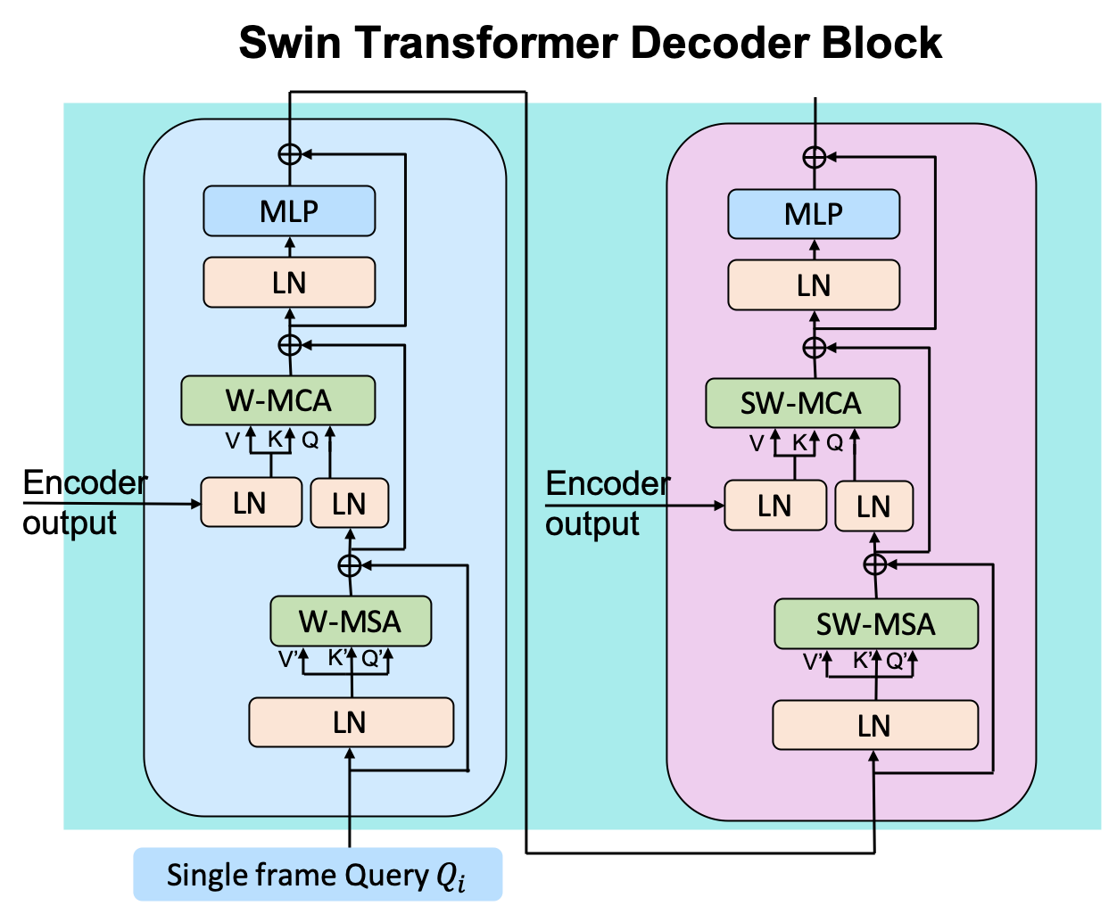
Figure 4: The basic Swin Transformer decoder block used in $\bm{D_{k},k=0,1,2,3}$ of RSTT; see Figure 2. It takes a query $Q$ and the output from the corresponding encoder $E_{k}$ as the input, and outputs HFR and HR features for spatial-temporal interpolation. Here, MCA stands for Multi-Head Cross-Attention, and other notations are similar to those in Figure 3.

Method	Vid4		Vimeo-Fast		Vimeo-Medium		Vimeo-Slow		FPS	Parameters
VFI+(V)SR/STVSR	PSNR$\uparrow$	SSIM$\uparrow$	PSNR$\uparrow$	SSIM$\uparrow$	PSNR$\uparrow$	SSIM$\uparrow$	PSNR$\uparrow$	SSIM$\uparrow$	$\uparrow$	(Millions) $\downarrow$
SuperSloMo [16] + Bicubic	22.84	0.5772	31.88	0.8793	29.94	0.8477	28.37	0.8102	-	19.8
SuperSloMo [16] + RCAN [61]	23.80	0.6397	34.52	0.9076	32.50	0.8884	30.69	0.8624	-	19.8+16.0
SuperSloMo [16] + RBPN [14]	23.76	0.6362	34.73	0.9108	32.79	0.8930	30.48	0.8584	-	19.8+12.7
SuperSloMo [16] + EDVR [49]	24.40	0.6706	35.05	0.9136	33.85	0.8967	30.99	0.8673	-	19.8+20.7
SepConv [33] + Bicubic	23.51	0.6273	32.27	0.8890	30.61	0.8633	29.04	0.8290	-	21.7
SepConv [33] + RCAN [61]	24.92	0.7236	34.97	0.9195	33.59	0.9125	32.13	0.8967	-	21.7+16.0
SepConv [33] + RBPN [14]	26.08	0.7751	35.07	0.9238	34.09	0.9229	32.77	0.9090	-	21.7+12.7
SepConv [33] + EDVR [49]	25.93	0.7792	35.23	0.9252	34.22	0.9240	32.96	0.9112	-	21.7+20.7
DAIN [1] + Bicubic	23.55	0.6268	32.41	0.8910	30.67	0.8636	29.06	0.8289	-	24.0
DAIN [1] + RCAN [61]	25.03	0.7261	35.27	0.9242	33.82	0.9146	32.26	0.8974	-	24.0+16.0
DAIN [1] + RBPN [14]	25.96	0.7784	35.55	0.9300	34.45	0.9262	32.92	0.9097	-	24.0+12.7
DAIN [1] + EDVR [49]	26.12	0.7836	35.81	0.9323	34.66	0.9281	33.11	0.9119	-	24.0+20.7
STARnet [15]	26.06	0.8046	36.19	0.9368	34.86	0.9356	33.10	0.9164	3.85	111.61
Zooming SlowMo [52]	26.31	0.7976	36.81	0.9415	35.41	0.9361	33.36	0.9138	15.59	11.10
TMNet [54]	26.43	0.8016	37.04	0.9435	35.60	0.9380	33.51	0.9159	14.33	12.26
RSTT-L	26.43	0.7994	36.80	0.9403	35.66	0.9381	33.50	0.9147	14.98	7.67
RSTT-M	26.37	0.7978	36.78	0.9401	35.62	0.9377	33.47	0.9143	19.07	6.08
RSTT-S	26.29	0.7941	36.58	0.9381	35.43	0.9358	33.30	0.9123	26.19	4.49

Table 1: Quantitative comparisons on various datasets with the state-of-the-art STVSR methods. PSNR and SSIM are computed on Y channel only, as same as [52]. Top three numbers of each column are bolded, with the best in red and the second best in blue. FPS is computed on Nvidia Quadro RTX 6000 machine and on Vid4 dataset, which has the output frame size of $720\times 576$.

3.3 Decoder

Same as the encoder part, we use four stages of decoders followed by a deconvolutional layer for feature up-sampling. The decoders $D_{k},k=0,1,2,3$ generate per-output-frame features in each level of details by repeatedly querying the dictionaries (the key-value pairs $(K,V)$ as shown in Figure 4) constructed from the encoders $E_{k}$’s in the same level. Each decoder consists of several (the same number as its corresponding encoder) Swin Transformer blocks, and each of the blocks takes two inputs: one is the output features from the encoder and the other is a single frame query, as shown in Figure 2 and Figure 4.

In RSTT, the first stage query $Q=\{Q_{i}\}_{i=1}^{7}$ for $D_{3}$ is interpolated from the the last encoder $E_{3}$ (see (3)) and the later queries are the outputs of the previous decoders. To generate seven HFR and HR output frames, each Swin Transformer decoder block queries the dictionary seven times. As a result, for a decoder contains $S$ such blocks, we need to query $7S$ times. In practice, the query is performed by Windowed Multi-Head Cross-Attention (W-MCA) [23] and its shifted version (SW-MCA) [23] (see Figure 4). Note that only the first Swin Transformer decoder block uses $Q$ as query while the rest $S-1$ blocks use the output of the previous block as query. Importantly, dictionaries provided by the encoders are pre-computed for reuse in each block. Suppose we have three Swin Transformer decoder blocks in each $D_{k}$, the spatial-temporal dictionaries built from the encoders are queried (reused) for $7\times 3=21$ times, which is advantageous over the duplication of future fusions in the existing approaches. This design is both computationally efficient and helpful in reducing the model size.

Final reconstruction module. The output features of the last decoder $D_{0}$ can be further processed by an optional reconstruction module to generate the final frames (see Figure 2). We use a module consisting of a 1-to-4 PixelShuffle operation and a single convolutional layer. This design is much more light-weight compared to the practices adopted in Zooming SlowMo [52] and TMNet [54], both of which use $40$ residual blocks to perform the spatial super resolution. We compare the performance of RSTT with and without such spatial reconstruction module in Section 4.3.

Ground-truth                               Ground-truth                  StarNet [15]         Zooming SlowMo [52]           TMNet [54]

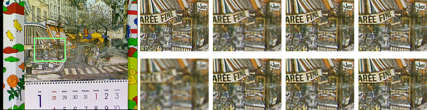
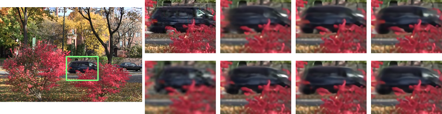
                                                          Overlaid                    RSTT-S                      RSTT-M                      RSTT-L
                 Ground-truth                               Ground-truth                  StarNet [15]         Zooming SlowMo [52]           TMNet [54]

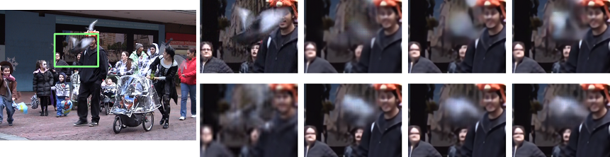
                                                          Overlaid                    RSTT-S                      RSTT-M                      RSTT-L
                 Ground-truth                               Ground-truth                  StarNet [15]         Zooming SlowMo [52]           TMNet [54]

                                                          Overlaid                    RSTT-S                      RSTT-M                      RSTT-L

Figure 5: Visual comparisons on the Vid4 dataset [21]. RSTT with three different sizes of architectures achieve the state-of-the-art performance in terms of visual qualities on various scenarios.

3.4 Training details

We train the proposed RSTT model using Adam with $\mathcal{L}_{2}$ and decoupled weight decay [25] by setting $\beta_{1}=0.9$ and $\beta_{2}=0.99$. The initial learning rate is set to $2\times 10^{-4}$ and is gradually decayed following the scheme of Cosine annealing with restart [13] set to $10^{-7}$. The restart performs at every 30,000 iterations. We train our model on two Nvidia Quadro RTX 6000 with batch size set to 7$\sim$10, depending on the particular model architecture.

Objective function. The Charbonnier loss is computed between the estimated frame $I^{H}$ and the ground truth $\hat{I}^{H}$:

$$L(\hat{I}^{H},I^{H})=\sqrt{\lVert\hat{I}^{H}-I^{H}\rVert^{2}+\epsilon^{2}},$$

where $\epsilon$ is set to $10^{-3}$ in our experiments.

Training dataset. We train our models on Vimeo-90K [57], which contains over 60,000 seven-frame video sequences. Many state-of-the-art methods [52, 53, 54] also use this dataset for training. For Vimeo-90K, the input LFR and LR frames are four frames of size $112\times 64$, and the output HFR and HR frames are seven frames of size $448\times 256$ (exactly $4\times$ larger in both height and width).

Evaluation. The models are evaluated on Vid4 [21] and Vimeo-90K [57] datasets. Vid4 is a small dataset consists of four video sequences of different scenes with $180\times 144$ input frames and $720\times 576$ output frames. Vimeo-90K validation set is split into fast, medium and slow motion sets as in [52] that contains 1225, 4972 and 1610 video clips.

4 Experiments

We train the proposed RSTT for three versions with small (S), medium (M) and large (L) architectures, corresponding to the number of Swin Transformer blocks used in each stage of encoder $E_{k}$ and decoder $D_{k}$ set to 2, 3 and 4, respectively. We term the three models as RSTT-S, RSTT-M and RSTT-L, and then compare them with other existing methods quantitatively and qualitatively.

4.1 Quantitative evaluation

We use Peak Signal to Noise Ratio (PSNR) and Structural Similarity (SSIM) as evaluation metrics for quantitative comparison. We also compare the model inference time in Frame Per Second (FPS) and model size in terms of the number of parameters, as shown in Table 1. We do not list the FPS of methods that sequentially apply separated VFI and VSR models, since they are much slower than the other competitors, as reported in [52, 54].

Method	Vid4		Vimeo-Fast		Vimeo-Medium		Vimeo-Slow		FPS	Parameters
VFI+(V)SR/STVSR	PSNR$\uparrow$	SSIM$\uparrow$	PSNR$\uparrow$	SSIM$\uparrow$	PSNR$\uparrow$	SSIM$\uparrow$	PSNR$\uparrow$	SSIM$\uparrow$	$\uparrow$	(Millions) $\downarrow$
RSTT-M-Recon	26.37	0.7988	36.80	0.9400	35.66	0.9381	33.58	0.9160	17.02	7.74
RSTT-M	26.37	0.7978	36.78	0.9401	35.62	0.9377	33.47	0.9143	19.07	6.08
RSTT-S-Recon	26.29	0.7951	36.56	0.9376	35.45	0.9361	33.40	0.9140	22.62	6.15
RSTT-S	26.29	0.7941	36.58	0.9381	35.43	0.9358	33.30	0.9123	26.19	4.49

Table 2: Quantitative comparisons of RSTT with and without the spatial reconstruction block. Top-three numbers of each column are bolded, with the best in red and the second best in blue.

We observe that all the RSTT models achieve state-of-the-art performance in both Vid4 and Vimeo-90K datasets with significantly smaller model size and substantially higher inference speed. Moreover, the performance grows steadily with increasing number of Swin Transformer blocks stacked in the architecture, from RSTT-S, -M to -L. Specifically, in Table 1, one can see that the smallest model RSTT-S performs similarly as Zooming SlowMo [52], while RSTT-M outperforms Zooming SlowMo [52] in Vid4, Vimeo-Medium and Vimeo-Slow with significantly smaller number of parameters and faster inference speed. Our largest model RSTT-L outperforms TMNet [54] on Vimeo-Medium, which is the largest dataset in Table 1, with $40\%$ smaller model size. We remark that our RSTT-S achieves a real-time rendering speed (more than 26 FPS) without sacrificing much performance.

4.2 Qualitative evaluation

We visually compare RSTT with other state-of-the art STVSR methods in Figure 5. We choose three different scenarios for the purpose of illustration:

• The first row shows the video of a still calendar in front of a moving camera. We observe that RSTT-S recovers details around the character. Texture details look more apparent compared with the result of StarNet [15].

• The second row shows the video taken by a still camera in the wild with fast moving vehicles. It is clear that RSTT outperforms StarNet [15] and Zooming SlowMo [52] with better contours of the moving vehicle.

• The third row illustrates a difficult case, where both the camera and the foreground objects are moving, especially the fast-flying pigeon. From the overlaid view, one can see that the pigeons in consecutive frames are barely overlapped. Our models give relatively better motion interpolations in this case compared with other state-of-the-arts. In addition, with the increasing sizes of our models, from RSTT-S to RSTT-L, we observe better interpolations.

4.3 Advantages of RSTT

We analyze the effectiveness of the Swin Transformer blocks used in encoders and decoders by comparing with using an optional spatial reconstruction block in Figure 2 with $10$ residual blocks (see Table 2). This block is similar to but smaller than the $40$ residual blocks used in Zooming SlowMo [52] and TMNet [54]. We observe that the additional reconstruction block only slightly changes the evaluation results. There are hardly any differences in performance ($\pm$0.02db in psnr) on Vid4, Vimeo-Fast and Vimeo-Medium datasets between RSTT models with and without adding reconstruction blocks. However, both the inference time and the network size are largely increased. Furthermore, RSTT-M (6.08M parameters) exhibits non-negligible improvement over RSTT-S-Recon (6.15M parameters) in all of the datasets ($\geq$0.2db in PSNR on Vimeo-Fast) with an even smaller model size. This reveals the effectiveness of our design, indicating larger spatial reconstruction block is unnecessary to RSTT. Note that we do not train a model with such additional block on RSTT-L due to the limited time, but we believe a similar pattern holds.

4.4 Limitations of RSTT

Long training time. Like other transformer-based methods [12], the required training time of RSTT is relatively long. It takes more than twenty-five days for convergence with the usage of two Nvidia Quadro RTX 6000 cards.

Lack the flexibility to interpolate at arbitrary time stamps. Unlike TMNet [54], RSTT lacks the flexibility of interpolating an intermediate frame at arbitrary time stamps since the Query $Q$ defined by (3) is fixed. However, we remark that this can be achieved by slightly rephrasing Query $Q$ for Decoder $D_{3}$. Suppose we would like to interpolate $n-1$ frames (at $n-1$ time stamps) between two frames, e.g., $E_{3,2t-1}$ and $E_{3,2t+1}$, we just need to make queries on $\{\frac{i}{n}E_{3,2t-1}+(1-\frac{i}{n})E_{3,2t+1}\}_{i=1}^{n-1}$ instead of $\frac{1}{2}E_{3,2t-1}+\frac{1}{2}E_{3,2t+1}$ where $n=2$ as a special case in (3). One might need to retrain the model to adopt such modifications, and we leave it as future work.

5 Conclusion

We presented a real-time spatial-temporal transformer (RSTT) for generating HFR and HR videos from LFR and LR ones. We considered to solve the space-time video super-resolution problem with a unified transformer architecture without having explicit separations of temporal and spatial sub-modules. Specifically, LFR and LR spatial-temporal features extracted from different levels of encoders are used to build dictionaries, which are then queried many times in the decoding stage for interpolating HFR and HR frames simultaneously. We emphasize that the key innovation of the work is the novel holistic formulation of self-attentions in encoders and cross-attentions in decoders. This holistic design leads to a significantly smaller model with much faster (real-time) inference speed compared with the state-of-the-art methods without noticeable difference in model performance.

Future directions along this line include but are not limited to: fusions of dictionaries built in different levels of encoders to make computations more efficient; controllable temporal super-resolution with the flexibility to interpolate frames at arbitrary time stamps; and sophisticated training loss functions that helps to improve the visual quality.

6 Supplementary Materials

6.1 Attention visualization

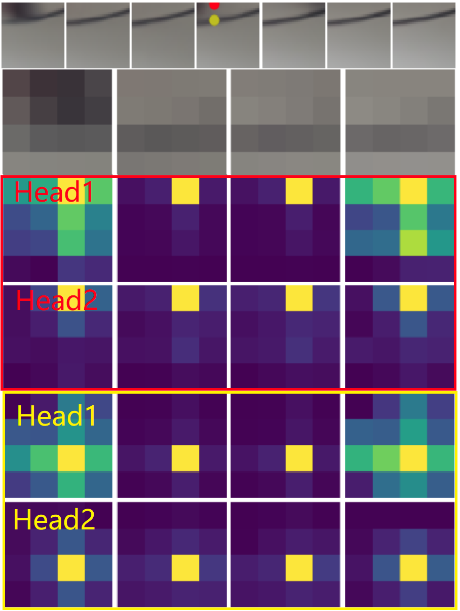
Figure 6: Windowed 2-Head attention of the last decoder.

To better understand the mechanism of RSTT, We show windowed 2-Head cross attentions of the last decoder on a sequence in Vimeo-Fast at two different locations (see Figure 6). Images bounded within red (yellow) box correspond to the red (yellow) dot highlighted in the outputs. We observe that the learnt attentions generally capture the local image structures in the finest level of detail.

6.2 Effectiveness of Multi-head Cross Attention

Decoder	Vid4		Vimeo-Fast
	PSNR$\uparrow$	SSIM$\uparrow$	PSNR$\uparrow$	SSIM$\uparrow$
MCA	26.29	0.7941	36.58	0.9381
Concat	26.18	0.7879	36.29	0.9346
Add	26.13	0.7865	36.25	0.9340

Table 3: Quantitative comparisons on Vid4 and Vimeo-Fast datasets between MCA and other information fusion methods. PSNR and SSIM are computed on Y channel only.

Decoder	Vimeo-Medium		Vimeo-Slow
	PSNR$\uparrow$	SSIM$\uparrow$	PSNR$\uparrow$	SSIM$\uparrow$
MCA	35.43	0.9358	33.30	0.9123
Concat	35.20	0.9332	33.15	0.9099
Add	35.15	0.9327	33.07	0.9090

Table 4: Quantitative comparisons on Vimeo-Medium and Vimeo-Slow datasets between MCA and other information fusion methods. PSNR and SSIM are computed on Y channel only.

RSTT employs Multi-head Cross Attention (MCA) to generate features in Decoders based on corresponding Encoders and Queries. To further investigate the effectiveness of this design, we replace MCA in RSTT-S with other ways of information combinations: concatenation and addition. The performance comparisons are shown in Table 3 and 4.

Here, both Windowed-MCA and Shifted Windowed-MCA are replaced by feature concatenation or feature addition by simply using 1d convolutions to match the feature sizes of stacked queries and the encoder outputs before this information fusion. Metrics in both Table 3 and 4 clearly testify the effectiveness of MCA over feature concatenation and feature addition.

References

- [1] Wenbo Bao, Wei-Sheng Lai, Chao Ma, Xiaoyun Zhang, Zhiyong Gao, and Ming-Hsuan Yang. Depth-aware video frame interpolation. In Proceedings of the IEEE Conference on Computer Vision and Pattern Recognition, pages 3703–3712, 2019.
- [2] Wenbo Bao, Wei-Sheng Lai, Xiaoyun Zhang, Zhiyong Gao, and Ming-Hsuan Yang. Memc-net: Motion estimation and motion compensation driven neural network for video interpolation and enhancement. IEEE transactions on pattern analysis and machine intelligence, 2019.
- [3] Tom B Brown, Benjamin Mann, Nick Ryder, Melanie Subbiah, Jared Kaplan, Prafulla Dhariwal, Arvind Neelakantan, Pranav Shyam, Girish Sastry, Amanda Askell, et al. Language models are few-shot learners. arXiv preprint arXiv:2005.14165, 2020.
- [4] Jose Caballero, Christian Ledig, Andrew Aitken, Alejandro Acosta, Johannes Totz, Zehan Wang, and Wenzhe Shi. Real-time video super-resolution with spatio-temporal networks and motion compensation. In Proceedings of the IEEE Conference on Computer Vision and Pattern Recognition, pages 4778–4787, 2017.
- [5] Hanting Chen, Yunhe Wang, Tianyu Guo, Chang Xu, Yiping Deng, Zhenhua Liu, Siwei Ma, Chunjing Xu, Chao Xu, and Wen Gao. Pre-trained image processing transformer. In Proceedings of the IEEE/CVF Conference on Computer Vision and Pattern Recognition, pages 12299–12310, 2021.
- [6] Xianhang Cheng and Zhenzhong Chen. Multiple video frame interpolation via enhanced deformable separable convolution. arXiv preprint arXiv:2006.08070, 2020.
- [7] Xianhang Cheng and Zhenzhong Chen. Video frame interpolation via deformable separable convolution. In AAAI, pages 10607–10614, 2020.
- [8] Michele Claus and Jan van Gemert. Videnn: Deep blind video denoising. In Proceedings of the IEEE/CVF Conference on Computer Vision and Pattern Recognition Workshops, pages 0–0, 2019.
- [9] Jifeng Dai, Haozhi Qi, Yuwen Xiong, Yi Li, Guodong Zhang, Han Hu, and Yichen Wei. Deformable convolutional networks. In Proceedings of the IEEE international conference on computer vision, pages 764–773, 2017.
- [10] Jacob Devlin, Ming-Wei Chang, Kenton Lee, and Kristina Toutanova. Bert: Pre-training of deep bidirectional transformers for language understanding. arXiv preprint arXiv:1810.04805, 2018.
- [11] Tianyu Ding, Luming Liang, Zhihui Zhu, and Ilya Zharkov. Cdfi: Compression-driven network design for frame interpolation. In Proceedings of the IEEE/CVF Conference on Computer Vision and Pattern Recognition, pages 8001–8011, 2021.
- [12] Alexey Dosovitskiy, Lucas Beyer, Alexander Kolesnikov, Dirk Weissenborn, Xiaohua Zhai, Thomas Unterthiner, Mostafa Dehghani, Matthias Minderer, Georg Heigold, Sylvain Gelly, Jakob Uszkoreit, and Neil Houlsby. An image is worth 16x16 words: Transformers for image recognition at scale. In International Conference on Learning Representations, 2021.
- [13] Akhilesh Gotmare, Nitish Shirish Keskar, Caiming Xiong, and Richard Socher. A closer look at deep learning heuristics: Learning rate restarts, warmup and distillation. In International Conference on Learning Representations (ICLR), 2018.
- [14] Muhammad Haris, Greg Shakhnarovich, and Norimichi Ukita. Recurrent back-projection network for video super-resolution. In IEEE Conference on Computer Vision and Pattern Recognition (CVPR), 2019.
- [15] Muhammad Haris, Greg Shakhnarovich, and Norimichi Ukita. Space-time-aware multi-resolution video enhancement. In IEEE Conference on Computer Vision and Pattern Recognition (CVPR), 2020.
- [16] Huaizu Jiang, Deqing Sun, Varun Jampani, Ming-Hsuan Yang, Erik Learned-Miller, and Jan Kautz. Super slomo: High quality estimation of multiple intermediate frames for video interpolation. In Proceedings of the IEEE Conference on Computer Vision and Pattern Recognition, pages 9000–9008, 2018.
- [17] Younghyun Jo, Seoung Wug Oh, Jaeyeon Kang, and Seon Joo Kim. Deep video super-resolution network using dynamic upsampling filters without explicit motion compensation. In 2018 IEEE/CVF Conference on Computer Vision and Pattern Recognition, pages 3224–3232, 2018.
- [18] Dahun Kim, Sanghyun Woo, Joon-Young Lee, and In So Kweon. Deep video inpainting. In Proceedings of the IEEE/CVF Conference on Computer Vision and Pattern Recognition, pages 5792–5801, 2019.
- [19] Hyeongmin Lee, Taeoh Kim, Tae-young Chung, Daehyun Pak, Yuseok Ban, and Sangyoun Lee. Adacof: Adaptive collaboration of flows for video frame interpolation. In Proceedings of the IEEE/CVF Conference on Computer Vision and Pattern Recognition, pages 5316–5325, 2020.
- [20] Jingyun Liang, Jiezhang Cao, Guolei Sun, Kai Zhang, Luc Van Gool, and Radu Timofte. Swinir: Image restoration using swin transformer. In Proceedings of the IEEE/CVF International Conference on Computer Vision, pages 1833–1844, 2021.
- [21] Ce Liu and Deqing Sun. A bayesian approach to adaptive video super resolution. In CVPR 2011, pages 209–216. IEEE, 2011.
- [22] Hongying Liu, Zhubo Ruan, Peng Zhao, Chao Dong, Fanhua Shang, Yuanyuan Liu, and Linlin Yang. Video super resolution based on deep learning: A comprehensive survey. arXiv preprint arXiv:2007.12928, 2020.
- [23] Ze Liu, Yutong Lin, Yue Cao, Han Hu, Yixuan Wei, Zheng Zhang, Stephen Lin, and Baining Guo. Swin transformer: Hierarchical vision transformer using shifted windows. In Proceedings of the IEEE/CVF International Conference on Computer Vision (ICCV), pages 10012–10022, October 2021.
- [24] Ziwei Liu, Raymond A Yeh, Xiaoou Tang, Yiming Liu, and Aseem Agarwala. Video frame synthesis using deep voxel flow. In Proceedings of the IEEE International Conference on Computer Vision, pages 4463–4471, 2017.
- [25] Ilya Loshchilov and Frank Hutter. Decoupled weight decay regularization. In International Conference on Learning Representations (ICLR), 2018.
- [26] Dhruv Mahajan, Fu-Chung Huang, Wojciech Matusik, Ravi Ramamoorthi, and Peter Belhumeur. Moving gradients: a path-based method for plausible image interpolation. ACM Transactions on Graphics (TOG), 28(3):1–11, 2009.
- [27] Simone Meyer, Abdelaziz Djelouah, Brian McWilliams, Alexander Sorkine-Hornung, Markus Gross, and Christopher Schroers. Phasenet for video frame interpolation. In Proceedings of the IEEE Conference on Computer Vision and Pattern Recognition, pages 498–507, 2018.
- [28] Simone Meyer, Oliver Wang, Henning Zimmer, Max Grosse, and Alexander Sorkine-Hornung. Phase-based frame interpolation for video. In Proceedings of the IEEE conference on computer vision and pattern recognition, pages 1410–1418, 2015.
- [29] Uma Mudenagudi, Subhashis Banerjee, and Prem Kumar Kalra. Space-time super-resolution using graph-cut optimization. IEEE Transactions on Pattern Analysis and Machine Intelligence, 33(5):995–1008, 2010.
- [30] Simon Niklaus and Feng Liu. Context-aware synthesis for video frame interpolation. In Proceedings of the IEEE Conference on Computer Vision and Pattern Recognition, pages 1701–1710, 2018.
- [31] Simon Niklaus and Feng Liu. Softmax splatting for video frame interpolation. In Proceedings of the IEEE/CVF Conference on Computer Vision and Pattern Recognition, pages 5437–5446, 2020.
- [32] Simon Niklaus, Long Mai, and Feng Liu. Video frame interpolation via adaptive convolution. In Proceedings of the IEEE Conference on Computer Vision and Pattern Recognition, pages 670–679, 2017.
- [33] Simon Niklaus, Long Mai, and Feng Liu. Video frame interpolation via adaptive separable convolution. In Proceedings of the IEEE International Conference on Computer Vision, pages 261–270, 2017.
- [34] Junheum Park, Keunsoo Ko, Chul Lee, and Chang-Su Kim. Bmbc: Bilateral motion estimation with bilateral cost volume for video interpolation. arXiv preprint arXiv:2007.12622, 2020.
- [35] René Ranftl, Alexey Bochkovskiy, and Vladlen Koltun. Vision transformers for dense prediction. In Proceedings of the IEEE/CVF International Conference on Computer Vision, pages 12179–12188, 2021.
- [36] Oren Rippel, Sanjay Nair, Carissa Lew, Steve Branson, Alexander G Anderson, and Lubomir Bourdev. Learned video compression. In Proceedings of the IEEE/CVF International Conference on Computer Vision, pages 3454–3463, 2019.
- [37] Mehdi SM Sajjadi, Raviteja Vemulapalli, and Matthew Brown. Frame-recurrent video super-resolution. In Proceedings of the IEEE Conference on Computer Vision and Pattern Recognition, pages 6626–6634, 2018.
- [38] Eli Shechtman, Yaron Caspi, and Michal Irani. Increasing space-time resolution in video. In European Conference on Computer Vision, pages 753–768. Springer, 2002.
- [39] Eli Shechtman, Yaron Caspi, and Michal Irani. Space-time super-resolution. IEEE Transactions on Pattern Analysis and Machine Intelligence, 27(4):531–545, 2005.
- [40] Zhihao Shi, Xiaohong Liu, Kangdi Shi, Linhui Dai, and Jun Chen. Video interpolation via generalized deformable convolution. arXiv preprint arXiv:2008.10680, 2020.
- [41] Robin Strudel, Ricardo Garcia, Ivan Laptev, and Cordelia Schmid. Segmenter: Transformer for semantic segmentation. arXiv preprint arXiv:2105.05633, 2021.
- [42] Benjamin Tag, Junichi Shimizu, Chi Zhang, Kai Kunze, Naohisa Ohta, and Kazunori Sugiura. In the eye of the beholder: The impact of frame rate on human eye blink. In Proceedings of the 2016 CHI Conference Extended Abstracts on Human Factors in Computing Systems, pages 2321–2327, 2016.
- [43] Xin Tao, Hongyun Gao, Renjie Liao, Jue Wang, and Jiaya Jia. Detail-revealing deep video super-resolution. In Proceedings of the IEEE International Conference on Computer Vision, pages 4472–4480, 2017.
- [44] Matias Tassano, Julie Delon, and Thomas Veit. Fastdvdnet: Towards real-time deep video denoising without flow estimation. In Proceedings of the IEEE/CVF Conference on Computer Vision and Pattern Recognition, pages 1354–1363, 2020.
- [45] Thierry Turletti and Christian Huitema. Videoconferencing on the internet. IEEE/ACM Transactions on networking, 4(3):340–351, 1996.
- [46] Ashish Vaswani, Noam Shazeer, Niki Parmar, Jakob Uszkoreit, Llion Jones, Aidan N Gomez, Łukasz Kaiser, and Illia Polosukhin. Attention is all you need. In Advances in neural information processing systems, pages 5998–6008, 2017.
- [47] Chuan Wang, Haibin Huang, Xiaoguang Han, and Jue Wang. Video inpainting by jointly learning temporal structure and spatial details. In Proceedings of the AAAI Conference on Artificial Intelligence, volume 33, pages 5232–5239, 2019.
- [48] Longguang Wang, Yulan Guo, Zaiping Lin, Xinpu Deng, and Wei An. Learning for video super-resolution through hr optical flow estimation. In Asian Conference on Computer Vision, pages 514–529. Springer, 2018.
- [49] Xintao Wang, Kelvin C.K. Chan, Ke Yu, Chao Dong, and Chen Change Loy. Edvr: Video restoration with enhanced deformable convolutional networks. In The IEEE Conference on Computer Vision and Pattern Recognition Workshops (CVPRW), June 2019.
- [50] Zhendong Wang, Xiaodong Cun, Jianmin Bao, and Jianzhuang Liu. Uformer: A general u-shaped transformer for image restoration. arXiv preprint arXiv:2106.03106, 2021.
- [51] Dapeng Wu, Yiwei Thomas Hou, Wenwu Zhu, Ya-Qin Zhang, and Jon M Peha. Streaming video over the internet: approaches and directions. IEEE Transactions on circuits and systems for video technology, 11(3):282–300, 2001.
- [52] Xiaoyu Xiang, Yapeng Tian, Yulun Zhang, Yun Fu, Jan P. Allebach, and Chenliang Xu. Zooming slow-mo: Fast and accurate one-stage space-time video super-resolution. In IEEE/CVF Conference on Computer Vision and Pattern Recognition (CVPR), pages 3370–3379, June 2020.
- [53] Xiaoyu Xiang, Yapeng Tian, Yulun Zhang, Yun Fu, Jan P Allebach, and Chenliang Xu. Zooming slowmo: An efficient one-stage framework for space-time video super-resolution, 2021.
- [54] Gang Xu, Jun Xu, Zhen Li, Liang Wang, Xing Sun, and Mingming Cheng. Temporal modulation network for controllable space-time video super-resolution. In IEEE/CVF Conference on Computer Vision and Pattern Recognition (CVPR), June 2021.
- [55] Haoran Xu, Benjamin Van Durme, and Kenton Murray. Bert, mbert, or bibert? a study on contextualized embeddings for neural machine translation. arXiv preprint arXiv:2109.04588, 2021.
- [56] Mengde Xu, Zheng Zhang, Han Hu, Jianfeng Wang, Lijuan Wang, Fangyun Wei, Xiang Bai, and Zicheng Liu. End-to-end semi-supervised object detection with soft teacher. arXiv preprint arXiv:2106.09018, 2021.
- [57] Tianfan Xue, Baian Chen, Jiajun Wu, Donglai Wei, and William T Freeman. Video enhancement with task-oriented flow. International Journal of Computer Vision, 127(8):1106–1125, 2019.
- [58] Jianwei Yang, Chunyuan Li, Pengchuan Zhang, Xiyang Dai, Bin Xiao, Lu Yuan, and Jianfeng Gao. Focal self-attention for local-global interactions in vision transformers. arXiv preprint arXiv:2107.00641, 2021.
- [59] Yun Fu Yapeng Tian, Yulun Zhang and Chenliang Xu. Tdan: Temporally deformable alignment network for video super-resolution. In IEEE/CVF Conference on Computer Vision and Pattern Recognition (CVPR), pages 3360–3369, June 2020.
- [60] Liangzhe Yuan, Yibo Chen, Hantian Liu, Tao Kong, and Jianbo Shi. Zoom-in-to-check: Boosting video interpolation via instance-level discrimination. In Proceedings of the IEEE Conference on Computer Vision and Pattern Recognition, pages 12183–12191, 2019.
- [61] Yulun Zhang, Kunpeng Li, Kai Li, Lichen Wang, Bineng Zhong, and Yun Fu. Image super-resolution using very deep residual channel attention networks. In ECCV, 2018.
- [62] Sixiao Zheng, Jiachen Lu, Hengshuang Zhao, Xiatian Zhu, Zekun Luo, Yabiao Wang, Yanwei Fu, Jianfeng Feng, Tao Xiang, Philip HS Torr, et al. Rethinking semantic segmentation from a sequence-to-sequence perspective with transformers. In Proceedings of the IEEE/CVF Conference on Computer Vision and Pattern Recognition, pages 6881–6890, 2021.
- [63] Chengcheng Zhou, Zongqing Lu, Linge Li, Qiangyu Yan, and Jing-Hao Xue. How Video Super-Resolution and Frame Interpolation Mutually Benefit, page 5445–5453. Association for Computing Machinery, New York, NY, USA, 2021.
- [64] Xizhou Zhu, Han Hu, Stephen Lin, and Jifeng Dai. Deformable convnets v2: More deformable, better results. In Proceedings of the IEEE Conference on Computer Vision and Pattern Recognition, pages 9308–9316, 2019.