A construction of exotic metallic states

Abstract

We discuss examples of two dimensional metallic states with charge fractionalization, and we will demonstrate that the mechanism of charge fractionalization leads to exotic metallic behaviors at low and intermediate temperature. The simplest example of such state is constructed by fermionic partons at finite density coupled to a $Z_{N}$ gauge field, whose properties can be studied through rudimentary methods. This simple state has the following exotic features: (1) at low temperature this state is a “bad metal” whose resistivity can be much larger than the Mott-Ioffe-Regel limit; (2) while increasing temperature $T$ the resistivity $\rho(T)$ is a nonmonotonic function, and it crosses over from a bad metal at low $T$ to a good metal at relatively high $T$; (3) the optical conductivity $\sigma(\omega)$ has a small Drude weight at low $T$, and a larger Drude weight at intermediate $T$; (4) at low temperature the metallic state has a large Lorenz number, which strongly violates the Wiedemann-Franz law. A more complex example with fermionic partons at finite density coupled to a ${\rm SU}(N)$ gauge field will also be constructed.

I Introduction

Dimensionless quantities in nature can be universal, meaning they are insensitive to the microscopic details of the system. Dimensionless universal quantities can arise from two different mechanisms: either criticality, or topology. At a critical point (either classical or quantum critical point), the diverging correlation length renders most of the the microscopic details irrelevant to infrared physics, hence each universality class is characterized by a series of numbers referred to as critical exponents. Examples of these critical points include various two dimensional statistical mechanics models such as the Ising model Yang (1952), the “Yang-Lee singularity” Lee and Yang (1952), and the Wilson-Fisher fixed points of three dimensional systems Wilson and Fisher (1972). Topology can lead to universal quantities due to topological quantization. The simplest example of such is the magnetic flux quantization in Dirac monopole Dirac (1931), and in superconductor Deaver and Fairbank (1961a, b). The Hall conductivity of quantum Hall systems (either integer or fractional) is a discrete universal number, it is related to the level of the Chern-Simons topological field theory Zhang et al. (1989); Wen and Niu (1990); ZHANG (1992); WEN (1990), which has to be quantized due to mathematical consistency.

Electrical resistivity/conductivity is a dimensionless quantity in two spatial dimensions, hence it can in principle take universal values that are independent of the microscopic details of the system. A universal resistivity can arise with various mechanisms. Besides the Hall resistivity of the quantum Hall states mentioned above, the resistivity of $(2+1)d$ quantum critical points with gapless charge degree of freedom Fisher et al. (1990); Cha et al. (1991), the resistivity jump at $(2+1)d$ metal-insulator transition driven by interaction Senthil (2008a, b); Witczak-Krempa et al. (2012), and the criterion of the so-called “bad metal” in two dimensions Hussey et al. (2004); Takagi et al. (1992); Emery and Kivelson (1995) are all “universal”. In all these examples, the resistivity (or the bound of resistivity) is always an order-unity dimensionless number times $h/e^{2}$.

This work concerns the metallic states with finite charge density and finite charge compressibility. The usual theory that describes the transport of a metal is the Boltzmann equation. The Boltzmann equation most conveniently applies when the concept of quasiparticles remains valid in the system , which usually requires that $l_{\mathrm{m}}k_{F}\gg 1$, where $l_{\mathrm{m}}$ is the mean free path, and $k_{F}$ is the Fermi wave vector. When $l_{\mathrm{m}}k_{F}$ becomes order 1, the resistivity saturates the Mott-Ioffe-Regel (MIR) limit of a metal, and the system becomes a “bad metal” Hussey et al. (2004); Takagi et al. (1992); Emery and Kivelson (1995), where descriptions based on quasiparticles break down. For a purely two dimensional system, the condition of $l_{\mathrm{m}}k_{F}\sim l_{\mathrm{m}}n^{1/2}\sim 1$ implies that the resistivity $\rho$ should be at the order of $h/e^{2}$. When the measured resistivity $\rho$ of a purely two dimensional metal is significantly larger than $h/e^{2}$, or in other words the estimated value of $l_{\mathrm{m}}k_{F}$ exceeds order unity for a $2d$ metal, one has to abandon the conventional description based on quasiparticles, and resort to other theoretical tools.

In real systems metallic states without quasiparticles usually arise from coupling electrons to bosonic gapless quantum critical modes. The theoretical formalism for these states usually start with a decoupled system with noninteracting electrons, and analyze how the fermion-boson coupling modifies the system Polchinski (1994); Nayak and Wilczek (1994a, b); Lee (2009); Mross et al. (2010); Metlitski and Sachdev (2010a, b). Through various perturbative renormalization group methods, one can show that the coupling between the Fermi surface and the gapless bosonic modes is relevant, and potentially drive the system into a non-Fermi liquid fixed point without quasiparticles. In recent years, a new route of constructing non-Fermi liquid has been explored, which was based on models that are soluble in certain limit (such as the Sachdev-Ye-Kitaev model and other related models) Sachdev and Ye (1993); Kitaev (2015); Maldacena and Stanford (2016); Witten (2016); Klebanov and Tarnopolsky (2017). These models have no notion of spatial dimensions, but solution of these models already have no quasiparticles. Lattice models built upon these soluble models quite naturally lead to non-Fermi liquids in various spatial dimensions Song et al. (2017); Werman et al. (2017); Werman and Berg (2016); Patel et al. (2018); Patel and Sachdev (2018); Chowdhury et al. (2018); Wu et al. (2018, 2019).

In this work we explore an alternative construction of exotic metallic states. The constructions used in this work are not based on soluble lattice models of interacting electrons, but there are sufficient theoretical arguments to show that these are indeed stable states. Though these examples are far from weakly interacting electrons with quasiparticles, the design of these states allows them to be studied through rudimentary theoretical tools.

II $Z_{N}$ fractionalized metal

The central idea of our construction is “charge fractionalization”. Fractionalization of quantum numbers is most well-known and well established in particle physics Gell-Mann (1964), but it is also predicted and observed in condensed matter systems such as fractional quantum Hall states Laughlin (1983); de Picciotto et al. (1997); Saminadayar et al. (1997). Quantum number fractionalization is also one of the signatory phenomena in quantum spin liquids Anderson (1973); Kalmeyer and Laughlin (1987); Wen et al. (1989); Read and Sachdev (1991); Wen (2002). Electric charge fractionalization was discussed in the context of Mott transition in systems with partially filled $3d$ pyrochlore lattice Chen et al. (2014). Recently, motivated by experiments on transition metal dichalcogenide (TMD) moiré heterostructures Li et al. (2021), effects of charge fractionalization at the metal-insulator transition in pure $2d$ systems have been discussed in Ref. Xu et al., 2021; Musser et al., 2021. In this work we will explore the consequences of charge fractionalization in a metallic state.

The first example we consider is a $Z_{N}$ topological order enriched with a global ${\rm U}(1)$ symmetry, which corresponds to the ordinary electric charge conservation. The elementary anyon $f_{\alpha}$ of the $Z_{N}$ topological order carries a $Z_{N}$ gauge charge, and it is also a spin-1/2 fermion with fractional electric charge $e_{*}=e/N$. When $N$ is an odd integer, the gauge invariant states of the system include fermions that carry odd integer electric charges and half-integer spins; as well as bosons with even integer charges and integer spins. This is the same Hilbert space as a many-body electron system.

It is known that the discrete gauge field at two spatial dimensions has a stable deconfined phase at zero temperature, in which the anyon $f_{\alpha}$ can be separated infinitely far from each other, hence the anyon $f_{\alpha}$ plays the role as the charge carriers in the system at least at zero temperature. Although we do not pursue an exactly soluble model based on electrons in this work, the state discussed here should be a stable state of electrons, given that a discrete gauge theory is free from confinement at zero temperature in $(2+1)d$. At finite temperature the thermal equilibrium state of the system is in a confined phase, but at low temperature the observable physics should still crossover to the deconfined phase at zero temperature. In fact, the finite temperature confinement of the $Z_{N}$ gauge field is caused by thermally activated population of gauge fluxes with nontrivial mutual statistics with $f_{\alpha}$. The confinement length $\xi(T)$, i.e. the distance that a single $f_{\alpha}$ can be separated from the “crowd”, takes the form of $\xi(T)\sim\exp(c\Delta/T)$, where $\Delta$ is the gap of $Z_{N}$ gauge fluxes, and $c$ is a constant. We argue that when $\xi(T)$ simultaneously satisfy two criteria, namely (i.) $\xi(T)$ is large compared with the distance between $f_{\alpha}$ anyons (assuming a sufficiently large charge density), and (ii.) $\xi(T)$ is large compared with the mean free path $l_{\mathrm{m}}$, the anyon $f_{\alpha}$ still plays the role of charge carrier in the nonequilibrium process of charge transport, as $f_{\alpha}$ does not travel long enough between two consecutive scatterings to “feel” the confinement.

— Charge Transport

In the follows we will discuss various properties of the state described above. We first consider electrical resistivity at zero temperature. The key advantage of this construction is that, at zero temperature, the $Z_{N}$ gauge field dynamics is gapped, and does not lead to any scattering to the gapless charged partons below the gap of the $Z_{N}$ gauge fields. The main source of relaxation of electric current at zero temperature still comes from conventional mechanisms, such as impurities, which give the partons a mean free length $l_{\mathrm{m}}$. If we assume the electric charge density is $en_{e}$, in an ordinary system without fractionalization, the rudimentary semiclassical theory of transport breaks down when $l_{\mathrm{m}}n_{e}^{1/2}\sim 1$, i.e. $l_{\mathrm{m}}\sim 1/n_{e}^{1/2}$. Since the parton carries charge $e/N$, the density of the parton is $n_{\ast}=Nn_{e}$, hence the usual transport theory can be applicable for even smaller $l_{\mathrm{m}}$, i.e. $l_{\mathrm{m}}\sim 1/(n_{\ast})^{1/2}\sim 1/(Nn_{e})^{1/2}$. When $l_{\mathrm{m}}$ saturates this limit, the system should be a “bad metal of partons”, with an “upper bound” of resistivity

$$\rho_{max}\sim\frac{h}{e_{*}^{2}}\sim N^{2}\frac{h}{e^{2}}.$$ (1)

When $l_{\mathrm{m}}\sim 1/(n_{\ast})^{1/2}>1$, rudimentary formalism of describing metallic states should still apply; the only difference is that now the charge carrier $f_{\alpha}$ carries charge $e_{\ast}=e/N$, and the density of $f_{\alpha}$ is higher than electric charge density.

At low temperature, a $2d$ $Z_{N}$ gauge field will cause confinement in equilibrium. As we mentioned above, the confinement of a $2d$ $Z_{N}$ gauge theory is caused by the thermally activated gauge fluxes, and the confinement length $\xi(T)$ is roughly the distance between two thermally activated gauge fluxes, hence $\xi(T)\sim\exp(c\Delta/T)$, where $\Delta$ is the energy gap for the $Z_{N}$ gauge flux. We need to compare $\xi(T)$ with other length scales of the system: the distance between anyons $f_{\alpha}$, which is given by $1/n_{\ast}^{1/2}$; the lattice constant $a$; and the mean free path $l_{\mathrm{m}}$. To ensure that the transport of the state can be studied with controlled methods, we assume that the mean free length $l_{\mathrm{m}}$ is at the order of, or larger than $N^{1/2}/n_{e}^{1/2}$; or equivalently $l_{\mathrm{m}}n_{\ast}^{1/2}$ is at the order of, or greater than $N$. In this limit, at least at low temperature, the following hierarchy of length scales holds: $\xi(T)>l_{\mathrm{m}}>1/n_{\ast}^{1/2}$. In this limit the simple theory of metal, such as the Drude formula still applies. The conductivity at zero and low temperature would be

$$\sigma_{0}=\frac{n_{\ast}e_{\ast}^{2}l_{\mathrm{m}}}{m_{\ast}v^{\ast}_{F}}\sim\frac{e_{\ast}^{2}}{h}(l_{\mathrm{m}}n_{\ast}^{1/2})\sim\frac{1}{N}\frac{e^{2}}{h},$$ (2)

which can still be a bad metal, even with the choice of relatively long mean free length.

We assume that $l_{\mathrm{m}}$ mostly arises from scattering with impurities with a hard-sphere like potential, and hence is insensitive to temperature. With rising temperature, the resistivity first increases with conventional mechanism, such as scattering with phonon, or interaction between the partons. These scattering are still suppressed due to the small electric charge carried by the partons. For example, the parton-phonon interaction is down by a factor of $1/N$ compared with the electron-phonon interaction, and the resistivity due to parton-phonon interaction is down by a factor of $1/N^{2}$. For short-range parton-parton interactions which presumably leads to Fermi liquid like scaling of resistivity (i.e. $\rho\sim\rho_{0}+AT^{2}$), if the short-range interaction arises from screened Coulomb interaction, the interaction is suppressed by a factor of $1/N^{2}$ .

When temperature rises further, the confinement length $\xi(T)$ becomes shorter, and eventually at temperature scale $T_{1}$ where $\xi(T_{1})\sim l_{\mathrm{m}}$, the semiclassical picture of $f_{\alpha}$ breaks down. At even higher temperature scale where the confinement length $\xi(T)$ is comparable with the lattice constant $a$, i.e. $T>T_{2}$ with $\xi(T_{2})\sim a$, the partons are fully confined, and the charge carriers should still be viewed as electrons. The electron density is $n_{e}$, and since we assumed a hard-sphere like potential of the impurities, $l_{\mathrm{m}}$ from impurities remains approximately unchanged from before. The conductivity at temperature $T_{2}$ should be

$$\sigma(T_{2})\sim\frac{n_{e}e^{2}l_{\mathrm{m}}}{mv_{F}}\sim N^{1/2}\frac{e^{2}}{h},$$ (3)

which can be a good metal. Hence with rising temperature, the resistivity evolves in a nonmonotonic way; it will crossover from a bad metal with $T<T_{1}$ to a good metal at $T\sim T_{2}$. The schematic behavior of $\rho(T)$ is sketched in Fig. 1.

We have chosen $l_{\mathrm{m}}$ so that the simple pictures of metal such as the Drude theory applies for both temperature ranges $T<T_{1}$ and $T>T_{2}$. In the low temperature range the semiclassical theory of metal with fractional charge carrier $f_{\alpha}$ becomes applicable; while with $T>T_{2}$ the system becomes a conventional metal with electrons. We lack the reliable theoretical tools to describe the intermediate temperature range $T_{1}<T<T_{2}$, but sufficient argument can lead to the conclusion that the system crossover from a bad metal phase at low temperature range, to a good metal phase in the higher temperature range. Also, if the optical conductivity is measured, our construction implies that the Drude weight of the optical conductivity is small at $T<T_{1}$, but the Drude weight will crossover to a larger value proportional to $\sigma(T_{2})$ at $T\sim T_{2}$.

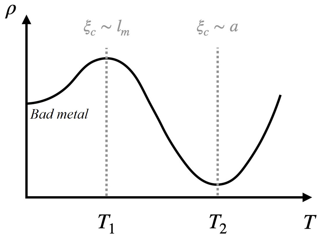
Figure 1: The schematic behavior of resistivity $\rho(T)$ constructed with fermionic partons carrying fractional charges coupled with a $Z_{N}$ gauge field.

— Hall Effect

For both temperature ranges $T<T_{1}$ and $T>T_{2}$, the transport coefficients can be derived with the rudimentary semiclassical theory of metal. We take the semiclassical Boltzmann transport equation under the relaxation-time approximation

$$\frac{\partial g}{\partial t}+\dot{\bm{x}}\cdot\frac{\partial g}{\partial\bm{x}}+\dot{\bm{k}}\cdot\frac{\partial g}{\partial\bm{k}}=\left(\frac{\partial g}{\partial t}\right)_{\textrm{coll}}\approx-\frac{\delta g}{\tau},$$ (4)

where $g(t,\bm{x},\bm{k})$ denotes the non-equilibrium distribution function, and $\delta g$ is its deviation from the equilibrium distribution $f(\epsilon)$. This Boltzman equation can be applied to the parton $f_{\alpha}$ at temperature $T<T_{1}$, and to electrons at temperature $T>T_{2}$.

At low temperature, according to the Ong’s formula Ong (1991) based on the Jones-Zener solution to Eq. 4, the weak-field Hall conductivity in $2d$ metals has a geometric interpretation

$$\sigma_{xy}=\frac{e_{*}^{2}}{h}\frac{\mathcal{A}_{l}}{\pi(l_{B}^{*})^{2}}$$ (5)

where $l_{B}^{*}=\sqrt{\hbar/(e_{*}B)}$ is the magnetic length for partons, and $\mathcal{A}_{l}$ is the area swept out by the vector $\bm{l}(\bm{k})=\tau(\epsilon(\bm{k}))\bm{v}(\bm{k})$ when $\bm{k}$ moves around the FS, i.e.,

$$\mathcal{A}_{l}=\frac{\bm{B}}{B}\cdot\int_{\textrm{FS}}d\bm{l}(\bm{k})\times\bm{l}(\bm{k})\sim l_{\textrm{m}}^{2}.$$ (6)

If we assume electrons and partons share the same isotropic $l_{\textrm{m}}$ and therefore the same area $\mathcal{A}_{l}$, there is a large ratio between $\sigma_{xy}$ at low temperature and the second crossover temperature $T_{2}$:

$$\frac{\sigma_{xy}(T_{2})}{\sigma_{xy}(T<T_{1})}\sim N^{3}.$$ (7)

The situation is different in the strong field limit. In this limit the collision integral in Eq. 4 can be neglected. Taking the directions $\bm{B}=B\hat{z}$ and $\bm{E}=E\hat{y}$, one obtains the solution $\delta g=(\hbar k_{x}E/B)(\partial f/\partial\epsilon)$ which has no explicit dependence on $N$. In this case, the integral of $v_{x}(\bm{k})\delta g(\bm{k})$ over the Brillouin zone gives $n_{*}E/B$, which leads to the high-field Hall conductivity

$$\sigma_{xy}=\frac{n_{\ast}e_{\ast}}{B}=\frac{n_{e}e}{B}.$$ (8)

The answer only depends on the total charge density.

— Thermoelectric Properties

In the presence of nonzero electric field $\bm{E}$ and temperature gradient $-\nabla T$, the linear response of electric current $\bm{J}^{e}$ and heat current $\bm{J}^{h}$ are usually organized in one equation

$$\left(\begin{array}[]{c}\bm{J}^{e}\\ \bm{J}^{h}\end{array}\right)=\left(\begin{array}[]{cc}\sigma&\alpha\\ T\alpha&\bar{\kappa}\end{array}\right)\left(\begin{array}[]{c}\bm{E}\\ -\nabla T\end{array}\right).$$ (15)

The electrical conductivity $\sigma$ and thermoelectric transport coefficients $\alpha,\bar{\kappa}$ are matrices of spatial coordinates. When $\bm{J}^{e}=0$, the thermal conductivity is given by $\kappa=\bar{\kappa}-T\alpha\sigma^{-1}\alpha$. The semiclassical equation of motion of partons in electric and magnetic fields reads

$$\dot{\bm{x}} \equiv\bm{v}_{n}(\bm{k})=\frac{1}{\hbar}\frac{\partial\epsilon_{n}(\bm{k})}{\partial\bm{k}}-\dot{\bm{k}}\times\bm{\Omega}_{n}(\bm{k}),$$

$$\hbar\dot{\bm{k}} =-e_{\ast}\bm{E}(\bm{x})-e_{\ast}\dot{\bm{x}}\times\bm{B}(\bm{x}),$$ (17)

where $n$ is the band index, and $\bm{\Omega}_{n}(\bm{k})$ is the Berry curvature associated with each band.

We first evaluate the diagonal thermoelectric response by neglecting the magnetic field $\bm{B}$ and the Berry curvature $\bm{\Omega}_{n}$. With nonzero electric field and temperature gradient, the solution of the Boltzmann equation Eq. 4 for deconfined partons reads

$$\delta g=-\left(e_{\ast}\bm{E}+\frac{\epsilon(\bm{k})-\mu}{T}\nabla T\right)\cdot\bm{v}(\bm{k})\tau(\epsilon(\bm{k}))\left(-\frac{\partial f}{\partial\epsilon}\right),$$ (18)

which leads to the diagonal transport coefficients

$$\sigma_{xx} =e_{*}^{2}\mathsf{s}_{xx}(\epsilon_{F}^{*})\sim\frac{\mathsf{s}_{xx}(\epsilon_{F}^{*})}{N^{2}},$$ (19)

$$\alpha_{xx} =-\frac{e_{*}}{T}\int d\epsilon\left(-\frac{\partial f}{\partial\epsilon}\right)(\epsilon-\mu)\mathsf{s}_{xx}(\epsilon)\sim\frac{T\mathsf{s}_{xx}^{\prime}(\epsilon_{F}^{*})}{N},$$

$$\bar{\kappa}_{xx} =\frac{1}{T}\int d\epsilon\left(-\frac{\partial f}{\partial\epsilon}\right)(\epsilon-\mu)^{2}\mathsf{s}_{xx}(\epsilon)\sim T\mathsf{s}_{xx}(\epsilon_{F}^{*}),$$

where we have used $(-\partial f/\partial\epsilon)\approx\delta(\epsilon-\epsilon_{F}^{*})$ and $\mu\approx\epsilon_{F}^{*}$ at low temperature, and the function $\mathsf{s}_{ij}(\epsilon)$ is defined as

$$\mathsf{s}_{ij}(\epsilon)=\tau(\epsilon)\int\frac{d^{2}\bm{k}}{(2\pi)^{2}}\delta(\epsilon-\epsilon(\bm{k}))v_{i}(\bm{k})v_{j}(\bm{k}).$$ (20)

Assuming the band mass is isotropic and $\bm{k}$-independent, one reproduces the Drude form for partons $\mathsf{s}_{ij}=\delta_{ij}\tau n_{*}/m_{*}$. The thermopower $Q$ (i.e., Seebeck coefficient) of the charge fractionalized metal is given by:

$$Q(T<T_{1})=\frac{\alpha_{xx}}{\sigma_{xx}}=-N\frac{\pi^{2}}{3}\frac{k_{B}^{2}T}{e}\frac{\sigma^{\prime}}{\sigma}.$$ (21)

Note that the mean free path $l_{\textrm{m}}$ gets cancelled in the ratio.

Experimentally, one clear signature for a charge fractionalized metal is the strong violation of the Wiedemann-Franz law. The Lorentz number acquires a large factor due to charge fractionalization:

$$L(T<T_{1})=\frac{\kappa_{xx}}{T\sigma_{xx}}=N^{2}\frac{\pi^{2}}{3}\frac{k_{B}^{2}}{e^{2}}.$$ (22)

This strong violation of the Wiedemann-Franz law can be naively understood by the fact that, though each fermionic parton carries a much smaller charge, it still carries the same entropy as an electron.

When the temperature reaches $T_{2}$ and the partons are fully confined, we expect these transport coefficients to decrease due to confinement

$$\frac{Q(T_{2})}{Q(T<T_{1})}\sim\frac{1}{N},\qquad\frac{L(T_{2})}{L(T<T_{1})}\sim\frac{1}{N^{2}}.$$ (23)

For systems that break time-reversal symmetry such as a ferromagnetic metal, the transport coefficients $\sigma,\alpha,\kappa$ could have nonzero off-diagonal terms even in the absence of $\bm{B}$. They receive intrinsic contributions from the Berry curvature in the band structure. Considering the nonzero Berry curvature $\bm{\Omega}(\bm{k})$ in Eq. 17, the parton wave packet acquires an anomalous velocity orthogonal to $\bm{E}$, which leads to the anomalous Hall conductivity

$$\sigma_{xy}(\epsilon)=\frac{e_{*}^{2}}{\hbar}\int\frac{d^{2}\bm{k}}{(2\pi)^{2}}\Theta(\epsilon-\epsilon(\bm{k}))\Omega^{z}(\bm{k}),$$ (24)

where $\Theta(\epsilon)$ is the Heaviside step function. Similar to their diagonal counterparts, the thermal Hall conductivity $\kappa_{xy}$ is given by

$$\kappa_{xy}(\epsilon)=\frac{\pi^{2}}{3}\frac{k_{B}^{2}T}{e_{*}^{2}}\sigma_{xy}(\epsilon).$$ (25)

At low temperature, the transverse Wiedemann-Franz law is still strongly violated due to charge fractionalization.

III Fractionalized metal with ${\rm SU}(N)$ gauge field

In this section we consider a more complex example of metal with charge fractionalization. For simplicity we will consider spin polarized electrons, hence the electron operator no longer carries a spin index. The first step of our construction is a parton construction:

$$c_{j}\sim\sum_{\{\alpha_{i}\}}\epsilon_{\alpha_{1},\alpha_{2},\cdots\alpha_{N}}f_{j,\alpha_{1}}f_{j,\alpha_{2}}\cdots f_{j,\alpha_{N}}.$$ (26)

This parton construction introduces a ${\rm SU}(N)$ gauge degree of freedom with an odd integer $N$. The nonabelian gauge field was also first introduced for particle physics Yang and Mills (1954), but later used broadly in the study of spin liquids (see for example Ref. Wen, 2002), and other strongly correlated electron systems Kaul et al. (2007); Xu and Sachdev (2010). The parton $f_{\alpha}$ with $\alpha=1\cdots N$ carries a fundamental representation of the ${\rm SU}(N)$ gauge group, and also physical electric charge $e_{*}=e/N$. The starting point of our analysis is the following Lagrangian:

$$\mathcal{L}_{\rm UV}\left[\Psi^{\dagger},\Psi,a\right]=\mathcal{L}_{{\rm UV},\left[\Psi,a\right]}+\mathcal{L}_{{\rm UV},a}$$

$$\mathcal{L}_{{\rm UV},\left[\Psi,a\right]}=\Psi^{\dagger}\left(\mathrm{i}\partial_{t}+ga_{0}^{I}t^{I}+e_{*}A_{0}+\mu\right)\Psi$$

$$\qquad\qquad\quad-\frac{1}{2m}\Psi^{\dagger}\left(-\mathrm{i}\partial_{i}+ga^{I}_{i}t^{I}+e_{*}A_{i}\right)^{2}\Psi$$

$$\mathcal{L}_{{\rm UV},a}=-\frac{1}{4}F^{I}_{\mu\nu}(F^{I})^{\mu\nu}$$ (27)

where $\Psi=(f_{1},f_{2},...,f_{N})^{t}$, $a^{I}_{\mu}=(a^{I}_{0},\ \vec{a}^{I})$ is the ${\rm SU}(N)$ gauge field with $\mu=0,1,2$; $t^{I}$ is the ${\rm SU}(N)$ Lie algebra in the fundamental representation, with $I=1,2,...,N^{2}-1$. $g$ is the strength of the gauge coupling, the non-Abelian gauge field stress tensor is $F^{I}_{\mu\nu}=\partial_{\mu}a_{\nu}^{I}-\partial_{\nu}a_{\mu}^{I}+g\mathsf{\epsilon}^{IJK}a^{J}_{\mu}a^{K}_{\nu}$; $A_{\mu}=(A_{0},\ \vec{A})$ is the background ${\rm U}(1)$ electromagnetic field.

Just like all systems that involve nonabelian gauge fields, Eq. (27) needs gauge fixing. The systematic method of gauge fixing is through the Faddeev-Popov procedure Faddeev and Popov (1967), by introducing the ghost fields. Since our system does not have Lorentz invariance to begin with, we will consider the Coulomb gauge $\bm{\nabla}\cdot\vec{a}=0$. It was shown in Ref. Zou and Chowdhury, 2020 that the ghost fields are decoupled from the system in the infrared limit. Further more, the nondynamical component of the gauge field $a_{0}$ is suppressed by the Thomas-Fermi screening of the Fermi surface, hence will be dropped in the rest of the consideration.

Eq. 27 with a finite Fermi surface is a highly challenging theory to study. Starting with the Lagrangian Eq. 27, one standard approximate treatment is to construct the low energy effective theory assuming that the Fermi energy is the largest energy scale in the problem, and $T\ll E_{F}$. Below the cutoff $\Lambda$ that satisfies $T\ll\Lambda\ll E_{F}$, the fermion operators can be expanded on two opposite patches of the Fermi surface. A patch model can be constructed following the logic of Ref. Polchinski, 1994; Nayak and Wilczek, 1994a, b; Lee, 2009; Mross et al., 2010; Metlitski and Sachdev, 2010a, b; Metlitski et al., 2015; Zou and Chowdhury, 2020. The patch lagrangian $\mathcal{L}_{{\rm patch},\left[\Psi,a\right]}$ reads

$$\mathcal{L}_{{\rm patch},\left[\Psi,a\right]} = \Psi^{\dagger}\left[\mathrm{i}\eta\partial_{t}-(lv_{F}k_{x}+\frac{k_{y}^{2}}{2m})\right]\Psi$$

$$- lgv_{F}\Psi^{\dagger}a_{x}^{I}t^{I}\Psi;$$

$$\mathcal{L}_{{\rm patch},a} = \frac{1}{2}q_{y}^{2}(a_{x}^{I})^{2}.$$ (31)

$x$ and $y$ are the local coordinates orthogonal and transverse to the patch Fermi surface of interest, $l=\pm 1$ labels the antipodal patches that can be connected by the transverse gauge fluctuations. The form of the patch Lagrangian implies the following scaling of space-time coordinates under coarse graining

$$\omega^{\prime}=b^{z_{f}}\omega,\ k^{\prime}_{x}=bk_{x},\ k^{\prime}_{y}=b^{1/2}k_{y}$$ (32)

with $z_{f}=1$, and $b>1$. Due to the different scaling dimensions of the $x$ and $y$ coordinate and the Coulomb gauge constraint, we find $\Delta_{a_{y}}=\Delta_{a_{x}}+1/2$, where $\Delta_{\mathcal{O}}$ is the scaling dimension of a field or coupling $\mathcal{O}$, e.g. $a^{\prime}_{y}=b^{\Delta_{a_{y}}}a_{y}$, $a^{\prime}_{x}=b^{\Delta_{a_{x}}}a_{x}$. Due to the highly anisotropic scaling of space-time, the form of the Lagrangian of the patch theory Eq. 31 is very different from a standard Lorentz invariant theory.

Unlike the ${\rm U}(1)$ gauge theory, a non-Abelian gauge field has self-interactions. It can be argued within the framework of the patch theory Zou and Chowdhury (2020) that the self-interaction between gauge bosons is irrelevant in the infrared, hence we can use Eq. 31 as the starting point of RG analysis. Note that the irrelevance of gauge field self-interactions is due to the highly anisotropic scaling of local coordinates $x$ and $y$ in Eq. 31. To get a controlled interacting RG fixed point, we need one more step of transformation of Eq. 31: we consider a small $\epsilon$ expansion by replacing $q_{y}^{2}$ with $q_{y}^{1+\epsilon}$, as was first introduced by Ref. Nayak and Wilczek, 1994a, b. At the leading order of $\epsilon$, only the 1-loop diagrams contribute, which leads to a weakly interacting RG fixed point Nayak and Wilczek (1994a, b); Mross et al. (2010). The self-energy correction to the parton propagator $\mathrm{G}=-\mathrm{i}\langle T_{t}\Psi\bar{\Psi}\rangle$ obtained by integrating out modes from $q_{y}=\Lambda$ to $q_{y}=\Lambda/b^{1/2}$ reads

$$\delta\Sigma=-\mathrm{i}\omega\frac{g^{2}v_{F}}{4\pi^{2}}\mathbb{c}_{2}\bm{1}\ln b$$ (33)

where $\mathbb{c}_{2}\bm{1}=\sum_{I}t^{I}t^{I}=\frac{N^{2}-1}{2N}\bm{1}$, with $\mathbb{c}_{2}$ the quadratic Casimir operator for the fundamental representation of ${\rm SU}(N)$; and $\bm{1}$ is the identity matrix in the color space. The vertex correction vanishes at the leading order $\epsilon$-expansion, as was argued in Ref. Mross et al., 2010. Eventually the one-loop corrections lead to a new fixed point $g_{*}^{2}=2\pi^{2}\epsilon/(\mathbb{c}_{2}v_{F})$. The existence of this fixed point is physically due to the screening of the gauge coupling from matter fields with finite density of states.

Physical properties at this new fixed point can be self-consistently solved. To be general, we consider the gauge field kinetic energy as $k_{y}^{2}\rightarrow|k_{y}|^{1+\epsilon}$, while $\epsilon$ is not necessarily small for the self-consistent calculation. Assuming that the parton self-energy does not depend on the momentum, which can be checked posteriori, the self-consistent equation reads

$$\Sigma_{\alpha\alpha^{\prime}}(\mathrm{i}\omega,\bm{k})=\sigma_{f}(\mathrm{i}\omega,\bm{k})\delta_{\alpha\alpha^{\prime}};$$ (36)

$$\sigma_{f}(\mathrm{i}\omega,\bm{k})=(-)g^{2}v_{F}^{2}\mathbb{c}_{2}$$

$$\times \int\frac{\mathrm{d}\nu\mathrm{d}q_{x}\mathrm{d}q_{y}}{(2\pi)^{3}}\frac{1}{\mathrm{i}(\omega+\nu)+\sigma_{f}(\omega+\nu)-\xi_{\bm{k}+\bm{q}}}$$ (38)

$$\times \frac{1}{\mathrm{i}\nu+\pi_{a}(\mathrm{i}\nu,\bm{q})+q_{y}^{1+\epsilon}};$$ (45)

$$\Pi_{IJ}(\mathrm{i}\nu,\bm{q})=\pi(\mathrm{i}\nu,\bm{q})\delta_{IJ};$$

$$\pi(\mathrm{i}\nu,\bm{q})=g^{2}v_{F}^{2}\mathbb{c}\int\frac{\mathrm{d}\bm{k}\mathrm{d}\omega}{(2\pi)^{3}}\frac{1}{\mathrm{i}\omega+\sigma_{f}(\omega)-\xi_{\bm{k}}}$$

$$\times \frac{1}{\mathrm{i}(\omega+\nu)+\sigma_{f}(\omega+\nu)-\xi_{\bm{k}+\bm{q}}}.$$ (47)

The solution for the fermion and gauge boson self-energy is

$$\mathrm{\Sigma}_{\alpha\alpha^{\prime}}(\omega) = -\mathrm{i}\frac{\mathbb{c}_{2}\mathbb{c}^{-\epsilon/(2+\epsilon)}}{2(8\pi)^{\epsilon/(2+\epsilon)}}\csc(\frac{2\pi}{2+\epsilon})\,\bar{g}^{\frac{2}{2+\epsilon}}E_{f}^{\frac{\epsilon}{2+\epsilon}}$$

$$\times |\omega|^{\frac{2}{2+\epsilon}}{\rm sgn}(\omega)\delta_{\alpha\alpha^{\prime}}$$

$$\pi(\mathrm{i}\nu,\bm{q}) = \frac{1}{v_{F}^{2+\epsilon}}\frac{\mathbb{c}}{8\pi}\bar{g}E_{f}^{1+\epsilon}\left|\frac{\nu}{\bm{q}}\right|.$$ (51)

Here we have defined a dimensionless coupling constant $\bar{g}=\frac{g^{2}v_{F}^{1-\epsilon}}{(2m)^{\epsilon}}$. One can see that the standard Landau damping term emerges in the self-consistent solution of the gauge boson self-energy. And the fermion self-energy takes the form of a non-Fermi liquid.

— Confinement and Crossover at finite temperature

To evaluate transport properties at different temperature scales, like the $Z_{N}$ gauge theory discussed earlier, we need to determine the two temperature scales $T_{1}$ and $T_{2}$ at which the confinement length satisfies $\xi_{c}(T_{1})\sim l_{\mathrm{m}}$ and $\xi_{c}(T_{2})\sim a$. When $\xi_{c}>l_{\mathrm{m}}$ the transport is governed by fractionalized charges. Like the case with the $Z_{N}$ gauge field, here we need to evaluate the scaling of $\xi_{c}$ with temperature at the fixed point discussed above, and in this section we are going to take $\epsilon=1$. First of all, the gauge fields would become classical when $g_{\ast}^{2}\frac{|\nu_{n=1}|}{q}>q^{2}$, where $\nu_{n}$ is the $n$-th Matsubara frequency. This gives a quantum-classical crossover length $\xi_{\rm cl}\sim q_{\rm cl}^{-1}\sim(Tg_{\ast}^{2})^{-\frac{1}{3}}$ above which the gauge field dynamics is classical. A classical gauge theory in $2d$ is described by the action

$$\mathcal{S}_{\rm classical}=\int\mathrm{d}\bm{x}\ \sum_{I}\frac{1}{Tg^{2}}(F^{I}_{\mu\nu})^{2}$$ (52)

The scaling dimension of $Tg^{2}$ now becomes $\Delta_{Tg^{2}}=2$. At the confinement length $\xi_{c}$, $Tg^{2}$ renormalizes to $Tg^{2}\sim 1$. We then find

$$\frac{Tg(\xi_{c})^{2}}{Tg_{\ast}^{2}}\sim\frac{1}{Tg_{\ast}^{2}}\sim\left(\frac{\xi_{c}}{\xi_{\rm cl}}\right)^{2}$$ (53)

$$\rightarrow \xi_{c}(T)\sim(Tg_{\ast}^{2})^{-5/6}\sim T^{-5/6}.$$ (55)

Hence at low temperature $T$, due to the Landau damping physics arising from the Fermi surface, when we observe the system with increasing length scale, physics of the gauge field will first crossover to classical at $\xi_{\rm cl}\sim(Tg_{\ast}^{2})^{-1/3}$, then crossover to confinement at an even longer scale $\xi_{c}(T)\sim(Tg_{\ast}^{2})^{-5/6}$. This analysis implies that the crossover temperature $T_{1}$ scales with the mean free path $T_{1}\sim l_{\mathrm{m}}^{-6/5}$.

— Transport Properties

At low temperature, we assume that the impurity still dominates the momentum relaxation. This assumption is valid at strictly zero temperature, and also valid at finite temperature with the artificial limit of small $\epsilon$, since the fixed point gauge coupling $g_{\ast}^{2}\sim\epsilon$, scattering with the gauge field is weak in this limit. The resistivity caused by gauge boson scattering can be computed following the procedure in Ref. Lee and Nagaosa, 1992. One key difference from the $Z_{N}$ example we discussed before is that, there are $N$ species of the fermionic partons now, each with the same density as the electron, and hence the same size of Fermi sea as the electron, $i.e.$ $n_{\ast}=n_{e}$, and $k_{F}^{\ast}=k_{F}$. In this case, the conductivity of the fractionalized metal at zero temperature reads

$$\sigma(T=0)=N\left(\frac{n_{\ast}e_{\ast}^{2}l_{\mathrm{m}}}{m_{\ast}v^{\ast}_{F}}\right)\sim\frac{1}{N}\frac{e^{2}}{h}(l_{\mathrm{m}}n_{e}^{1/2}),$$ (56)

which can still be a bad metal. Notice that in other parton constructions for example in Ref. Senthil, 2008a, the total electrical conductivity is governed by the Ioeffe-Larkin rule Ioffe and Larkin (1989); while in our case the conductivity should be a direct sum of conductivity of each parton. Once again, when the confinement length $\xi_{c}$ becomes the order of lattice constant $a$ (which occurs at temperature $T_{2}$ with $\xi_{c}(T_{2})\sim a$ ), the partons are fully confined to electron, and the conductivity is given by the standard form $\sigma(T_{2})=\frac{e^{2}}{h}(l_{\mathrm{m}}n_{e}^{1/2})$.

At low temperature, both the partons and the gauge bosons will contribute to the thermal transport. But it was shown that the gauge boson contribution is subdominant Nave and Lee (2007) compared with the fermionic partons, hence it will be ignored in the following discussion. At low temperature the thermal transport of the fermionic partons will also be mostly determined by their scattering with impurities:

$$\frac{\kappa}{T}=N\left(\frac{\pi^{2}}{3}\frac{k_{B}^{2}n_{\ast}l_{\mathrm{m}}}{m_{\ast}v_{F}^{\ast}}\right)\sim N\frac{\pi^{2}}{3}\frac{k_{B}^{2}}{h}(l_{\mathrm{m}}n_{e}^{1/2}),$$ (57)

again we have taken into account of the fact that, there are $N$ color species of the partons, and for each species $n_{\ast}=n_{e}$. There is still a strong violation of the Wiedmann Franz law same as the $Z_{N}$ gauge field case Eq. (22) at zero temperature:

$$L(T=0)=\frac{\kappa_{xx}}{T\sigma_{xx}}=N^{2}\frac{\pi^{2}}{3}\frac{k_{B}^{2}}{e^{2}}.$$ (58)

IV Summary and Discussion

We proposed two constructions of exotic metallic phases based on the idea of charge fractionalization. It was proposed before that charge fractionalization may be playing an important role Xu et al. (2021) in the metal-insulator transition (MIT) observed in transition metal dichalcogenide (TMD) moiré heterostructures Li et al. (2021), where an anomalously large resistivity was observed at low temperature near and at the MIT, followed by a rapid drop of resistivity at slightly higher temperature, analogous to the physics discussed between $T_{1}$ and $T_{2}$ in Fig. 1. Similar physics has also been observed in another TMD moiré sample Zhang et al. (2022).

The two constructions discussed in this work are actually related to each other. The ${\rm SU}(N)$ gauge group always has a $Z_{N}$ center, hence the ${\rm SU}(N)$ gauge field can be broken down to a $Z_{N}$ gauge field by condensing Higgs fields Higgs (1964); Englert and Brout (1964); Guralnik et al. (1964) with the right representation. The condensed Higgs field is also expected to mix the different color species and lift the degeneracy of the fermionic parton Fermi surface. In fact, a spin liquid usually has a ${\rm U}(1)$ or even ${\rm SU}(2)$ gauge degrees of freedom in the UV, but the gauge group can be broken down to $Z_{2}$ through the Higgs mechanism, hence in the infrared the system becomes a $Z_{2}$ spin liquid Wen et al. (1989); Read and Sachdev (1991); Wen (2002).

Xu’s group is supported by NSF Grant No. DMR-1920434, and the Simons Investigator program; Z.L.is supported by the Simons Collaborations on Ultra-Quantum Matter, grant 651440 (LB); M.Y. was supported in part by the Gordon and Betty Moore Foundation through Grant GBMF8690 to UCSB, and by the NSF Grant No. PHY-1748958. The authors thank Chao-Ming Jian for very helpful discussions.

References

- Yang (1952) C. N. Yang, Phys. Rev. 85, 808 (1952), URL https://link.aps.org/doi/10.1103/PhysRev.85.808.
- Lee and Yang (1952) T. D. Lee and C. N. Yang, Phys. Rev. 87, 410 (1952), URL https://link.aps.org/doi/10.1103/PhysRev.87.410.
- Wilson and Fisher (1972) K. G. Wilson and M. E. Fisher, Phys. Rev. Lett. 28, 240 (1972), URL https://link.aps.org/doi/10.1103/PhysRevLett.28.240.
- Dirac (1931) P. A. M. Dirac, Proceedings of the Royal Society of London. Series A, Containing Papers of a Mathematical and Physical Character 133, 60 (1931), eprint https://royalsocietypublishing.org/doi/pdf/10.1098/rspa.1931.0130, URL https://royalsocietypublishing.org/doi/abs/10.1098/rspa.1931.%0130.
- Deaver and Fairbank (1961a) B. S. Deaver and W. M. Fairbank, Phys. Rev. Lett. 7, 43 (1961a), URL https://link.aps.org/doi/10.1103/PhysRevLett.7.43.
- Deaver and Fairbank (1961b) B. S. Deaver and W. M. Fairbank, Phys. Rev. Lett. 7, 43 (1961b), URL https://link.aps.org/doi/10.1103/PhysRevLett.7.43.
- Zhang et al. (1989) S. C. Zhang, T. H. Hansson, and S. Kivelson, Phys. Rev. Lett. 62, 82 (1989), URL https://link.aps.org/doi/10.1103/PhysRevLett.62.82.
- Wen and Niu (1990) X. G. Wen and Q. Niu, Phys. Rev. B 41, 9377 (1990), URL https://link.aps.org/doi/10.1103/PhysRevB.41.9377.
- ZHANG (1992) S. C. ZHANG, International Journal of Modern Physics B 06, 25 (1992), eprint https://doi.org/10.1142/S0217979292000037, URL https://doi.org/10.1142/S0217979292000037.
- WEN (1990) X. G. WEN, International Journal of Modern Physics B 04, 239 (1990), eprint https://doi.org/10.1142/S0217979290000139, URL https://doi.org/10.1142/S0217979290000139.
- Fisher et al. (1990) M. P. A. Fisher, G. Grinstein, and S. M. Girvin, Phys. Rev. Lett. 64, 587 (1990), URL https://link.aps.org/doi/10.1103/PhysRevLett.64.587.
- Cha et al. (1991) M.-C. Cha, M. P. A. Fisher, S. M. Girvin, M. Wallin, and A. P. Young, Phys. Rev. B 44, 6883 (1991), URL https://link.aps.org/doi/10.1103/PhysRevB.44.6883.
- Senthil (2008a) T. Senthil, Phys. Rev. B 78, 035103 (2008a), URL https://link.aps.org/doi/10.1103/PhysRevB.78.035103.
- Senthil (2008b) T. Senthil, Phys. Rev. B 78, 045109 (2008b), URL https://link.aps.org/doi/10.1103/PhysRevB.78.045109.
- Witczak-Krempa et al. (2012) W. Witczak-Krempa, P. Ghaemi, T. Senthil, and Y. B. Kim, Phys. Rev. B 86, 245102 (2012), URL https://link.aps.org/doi/10.1103/PhysRevB.86.245102.
- Hussey et al. (2004) N. E. Hussey, K. Takenaka, and H. Takagi, Philosophical Magazine 84, 2847 (2004), eprint https://doi.org/10.1080/14786430410001716944, URL https://doi.org/10.1080/14786430410001716944.
- Takagi et al. (1992) H. Takagi, B. Batlogg, H. L. Kao, J. Kwo, R. J. Cava, J. J. Krajewski, and W. F. Peck, Phys. Rev. Lett. 69, 2975 (1992), URL https://link.aps.org/doi/10.1103/PhysRevLett.69.2975.
- Emery and Kivelson (1995) V. J. Emery and S. A. Kivelson, Phys. Rev. Lett. 74, 3253 (1995), URL https://link.aps.org/doi/10.1103/PhysRevLett.74.3253.
- Polchinski (1994) J. Polchinski, Nuclear Physics B 422, 617 (1994), ISSN 0550-3213, URL http://www.sciencedirect.com/science/article/pii/055032139490%4499.
- Nayak and Wilczek (1994a) C. Nayak and F. Wilczek, Nuclear Physics B 417, 359 (1994a), ISSN 0550-3213, URL http://www.sciencedirect.com/science/article/pii/055032139490%4774.
- Nayak and Wilczek (1994b) C. Nayak and F. Wilczek, Nuclear Physics B 430, 534 (1994b), ISSN 0550-3213, URL http://www.sciencedirect.com/science/article/pii/055032139490%1589.
- Lee (2009) S.-S. Lee, Phys. Rev. B 80, 165102 (2009), URL https://link.aps.org/doi/10.1103/PhysRevB.80.165102.
- Mross et al. (2010) D. F. Mross, J. McGreevy, H. Liu, and T. Senthil, Phys. Rev. B 82, 045121 (2010), URL https://link.aps.org/doi/10.1103/PhysRevB.82.045121.
- Metlitski and Sachdev (2010a) M. A. Metlitski and S. Sachdev, Phys. Rev. B 82, 075127 (2010a), URL https://link.aps.org/doi/10.1103/PhysRevB.82.075127.
- Metlitski and Sachdev (2010b) M. A. Metlitski and S. Sachdev, Phys. Rev. B 82, 075128 (2010b), URL https://link.aps.org/doi/10.1103/PhysRevB.82.075128.
- Sachdev and Ye (1993) S. Sachdev and J. Ye, Physical Review Letters 70, 3339 (1993), eprint cond-mat/9212030.
- Kitaev (2015) A. Kitaev, A simple model of quantum holography, http://online.kitp.ucsb.edu/online/entangled15/kitaev/,http://online.kitp.ucsb.edu/online/entangled15/kitaev2/. (2015), Talks at KITP, April 7, 2015 and May 27, 2015.
- Maldacena and Stanford (2016) J. Maldacena and D. Stanford, Phys. Rev. D 94, 106002 (2016), eprint 1604.07818.
- Witten (2016) E. Witten, ArXiv e-prints (2016), eprint 1610.09758.
- Klebanov and Tarnopolsky (2017) I. R. Klebanov and G. Tarnopolsky, Phys. Rev. D 95, 046004 (2017), URL https://link.aps.org/doi/10.1103/PhysRevD.95.046004.
- Song et al. (2017) X.-Y. Song, C.-M. Jian, and L. Balents, Phys. Rev. Lett. 119, 216601 (2017), URL https://link.aps.org/doi/10.1103/PhysRevLett.119.216601.
- Werman et al. (2017) Y. Werman, S. A. Kivelson, and E. Berg, npj Quantum Materials 2 (2017), ISSN 2397-4648, URL http://dx.doi.org/10.1038/s41535-017-0009-8.
- Werman and Berg (2016) Y. Werman and E. Berg, Phys. Rev. B 93, 075109 (2016), URL https://link.aps.org/doi/10.1103/PhysRevB.93.075109.
- Patel et al. (2018) A. A. Patel, J. McGreevy, D. P. Arovas, and S. Sachdev, Phys. Rev. X 8, 021049 (2018), URL https://link.aps.org/doi/10.1103/PhysRevX.8.021049.
- Patel and Sachdev (2018) A. A. Patel and S. Sachdev, Phys. Rev. B 98, 125134 (2018), URL https://link.aps.org/doi/10.1103/PhysRevB.98.125134.
- Chowdhury et al. (2018) D. Chowdhury, Y. Werman, E. Berg, and T. Senthil, Phys. Rev. X 8, 031024 (2018), URL https://link.aps.org/doi/10.1103/PhysRevX.8.031024.
- Wu et al. (2018) X. Wu, X. Chen, C.-M. Jian, Y.-Z. You, and C. Xu, Phys. Rev. B 98, 165117 (2018), URL https://link.aps.org/doi/10.1103/PhysRevB.98.165117.
- Wu et al. (2019) X.-C. Wu, C.-M. Jian, and C. Xu, Phys. Rev. B 100, 075101 (2019), URL https://link.aps.org/doi/10.1103/PhysRevB.100.075101.
- Gell-Mann (1964) M. Gell-Mann, Physics Letters 8, 214 (1964), ISSN 0031-9163, URL https://www.sciencedirect.com/science/article/pii/S0031916364%920013.
- Laughlin (1983) R. B. Laughlin, Phys. Rev. Lett. 50, 1395 (1983), URL https://link.aps.org/doi/10.1103/PhysRevLett.50.1395.
- de Picciotto et al. (1997) R. de Picciotto, M. Reznikov, M. Heiblum, V. Umansky, G. Bunin, and D. Mahalu, Nature 389, 162 (1997).
- Saminadayar et al. (1997) L. Saminadayar, D. C. Glattli, Y. Jin, and B. Etienne, Phys. Rev. Lett. 79, 2526 (1997), URL https://link.aps.org/doi/10.1103/PhysRevLett.79.2526.
- Anderson (1973) P. Anderson, Materials Research Bulletin 8, 153 (1973), ISSN 0025-5408, URL https://www.sciencedirect.com/science/article/pii/00255408739%01670.
- Kalmeyer and Laughlin (1987) V. Kalmeyer and R. B. Laughlin, Phys. Rev. Lett. 59, 2095 (1987), URL https://link.aps.org/doi/10.1103/PhysRevLett.59.2095.
- Wen et al. (1989) X. G. Wen, F. Wilczek, and A. Zee, Phys. Rev. B 39, 11413 (1989), URL https://link.aps.org/doi/10.1103/PhysRevB.39.11413.
- Read and Sachdev (1991) N. Read and S. Sachdev, Phys. Rev. Lett. 66, 1773 (1991), URL https://link.aps.org/doi/10.1103/PhysRevLett.66.1773.
- Wen (2002) X.-G. Wen, Phys. Rev. B 65, 165113 (2002), URL https://link.aps.org/doi/10.1103/PhysRevB.65.165113.
- Chen et al. (2014) G. Chen, H.-Y. Kee, and Y. B. Kim, Phys. Rev. Lett. 113, 197202 (2014), URL https://link.aps.org/doi/10.1103/PhysRevLett.113.197202.
- Li et al. (2021) T. Li, S. Jiang, L. Li, Y. Zhang, K. Kang, J. Zhu, K. Watanabe, T. Taniguchi, D. Chowdhury, L. Fu, et al., Nature 597, 350C354 (2021), ISSN 1476-4687, URL http://dx.doi.org/10.1038/s41586-021-03853-0.
- Xu et al. (2021) Y. Xu, X.-C. Wu, M.-X. Ye, Z.-X. Luo, C.-M. Jian, and C. Xu, Metal-insulator transition with charge fractionalization (2021), eprint 2106.14910.
- Musser et al. (2021) S. Musser, T. Senthil, and D. Chowdhury, Theory of a continuous bandwidth-tuned wigner-mott transition (2021), eprint 2111.09894.
- Ong (1991) N. P. Ong, Phys. Rev. B 43, 193 (1991), URL https://link.aps.org/doi/10.1103/PhysRevB.43.193.
- Yang and Mills (1954) C. N. Yang and R. L. Mills, Phys. Rev. 96, 191 (1954), URL https://link.aps.org/doi/10.1103/PhysRev.96.191.
- Kaul et al. (2007) R. K. Kaul, Y. B. Kim, S. Sachdev, and T. Senthil, Nature Physics 4, 28 (2007), URL https://doi.org/10.1038%2Fnphys790.
- Xu and Sachdev (2010) C. Xu and S. Sachdev, Phys. Rev. Lett. 105, 057201 (2010), URL https://link.aps.org/doi/10.1103/PhysRevLett.105.057201.
- Faddeev and Popov (1967) L. Faddeev and V. Popov, Physics Letters B 25, 29 (1967), ISSN 0370-2693, URL https://www.sciencedirect.com/science/article/pii/03702693679%00676.
- Zou and Chowdhury (2020) L. Zou and D. Chowdhury, Phys. Rev. Research 2, 023344 (2020), URL https://link.aps.org/doi/10.1103/PhysRevResearch.2.023344.
- Metlitski et al. (2015) M. A. Metlitski, D. F. Mross, S. Sachdev, and T. Senthil, Phys. Rev. B 91, 115111 (2015), URL https://link.aps.org/doi/10.1103/PhysRevB.91.115111.
- Lee and Nagaosa (1992) P. A. Lee and N. Nagaosa, Phys. Rev. B 46, 5621 (1992), URL https://link.aps.org/doi/10.1103/PhysRevB.46.5621.
- Ioffe and Larkin (1989) L. B. Ioffe and A. I. Larkin, Phys. Rev. B 39, 8988 (1989), URL https://link.aps.org/doi/10.1103/PhysRevB.39.8988.
- Nave and Lee (2007) C. P. Nave and P. A. Lee, Phys. Rev. B 76, 235124 (2007), URL https://link.aps.org/doi/10.1103/PhysRevB.76.235124.
- Zhang et al. (2022) M. Zhang, X. Zhao, K. Watanabe, T. Taniguchi, Z. Zhu, F. Wu, Y. Li, and Y. Xu, Pomeranchuk effect and tunable quantum phase transitions in 3l-mote2/wse2 (2022), URL https://arxiv.org/abs/2203.01010.
- Higgs (1964) P. W. Higgs, Phys. Rev. Lett. 13, 508 (1964), URL https://link.aps.org/doi/10.1103/PhysRevLett.13.508.
- Englert and Brout (1964) F. Englert and R. Brout, Phys. Rev. Lett. 13, 321 (1964), URL https://link.aps.org/doi/10.1103/PhysRevLett.13.321.
- Guralnik et al. (1964) G. S. Guralnik, C. R. Hagen, and T. W. B. Kibble, Phys. Rev. Lett. 13, 585 (1964), URL https://link.aps.org/doi/10.1103/PhysRevLett.13.585.
- Kim et al. (1995) Y. B. Kim, P. A. Lee, and X.-G. Wen, Phys. Rev. B 52, 17275 (1995), URL https://link.aps.org/doi/10.1103/PhysRevB.52.17275.