NUNet: Deep Learning for Non-Uniform Super-Resolution of Turbulent Flows

Abstract

Deep Learning (DL) algorithms are becoming increasingly popular for the reconstruction of high-resolution turbulent flows (aka super-resolution). However, current DL approaches perform spatially uniform super-resolution – a key performance limiter for scalability of DL-based surrogates for Computational Fluid Dynamics (CFD).

To address the above challenge, we introduce NUNet, a deep learning-based adaptive mesh refinement (AMR) framework for non-uniform super-resolution of turbulent flows. NUNet divides the input low-resolution flow field into patches, scores each patch, and predicts their target resolution. As a result, it outputs a spatially non-uniform flow field, adaptively refining regions of the fluid domain to achieve the target accuracy. We train NUNet with Reynolds-Averaged Navier-Stokes (RANS) solutions from three different canonical flows, namely turbulent channel flow, flat plate, and flow around ellipses. NUNet shows remarkable discerning properties, refining areas with complex flow features, such as near-wall domains and the wake region in flow around solid bodies, while leaving areas with smooth variations (such as the freestream) in the low-precision range. Hence, NUNet demonstrates an excellent qualitative and quantitative alignment with the traditional OpenFOAM AMR solver. Moreover, it reaches the same convergence guarantees as the AMR solver while accelerating it by $3.2-5.5\times$, including unseen-during-training geometries and boundary conditions, demonstrating its generalization capacities. Due to NUNet’s ability to super-resolve only regions of interest, it predicts the same target $1024\times 1024$ spatial resolution $7-28.5\times$ faster than state-of-the-art DL methods and reduces the memory usage by $4.4-7.65\times$, showcasing improved scalability.

Keywords Adaptive mesh refinement, deep learning, superresolution, turbulent flows

1 Introduction

Computational Fluid Dynamics (CFD) is the de-facto method for solving the Navier-Stokes equations, a set of Partial Differential Equations (PDEs), both for laminar and turbulent flow problems [1, 2, 3, 4, 5, 6]. Practical turbulent CFD simulations require high spatial resolutions (such as 1024 $\times$ 1024 [7]), making these simulations computationally expensive. There are widespread efforts to address this challenge and improve the performance and scalability of solving these systems [8, 9, 10] for faster design space exploration. Inspired by the remarkable success of deep learning (DL) algorithms in both computer vision (CV) [11] and natural language processing (NLP) [12], recent works have leveraged DL algorithms for accelerating CFD simulations via super-resolution, that is, reconstructing expensive high-resolution (HR) solutions from their cost-effective low-resolution (LR) counterpart [13, 14, 15, 16, 17].

State-of-the-art (SOTA) DL models for super-resolution have shown promise as domain-agnostic models and real-time predictors that can generalize to a broad set of flow configurations and conditions. However, they all suffer from the fundamental limitation of performing uniform super-resolution, that is, every pixel of the input LR image is refined to the target high resolution. As a result, SOTA [16, 13, 15] methods for super-resolution need higher computational resources - increased inference times and memory requirements - since the target high-resolution solution is output in the entire physical domain. Figure 1 shows the maximum allowable batch size with increasing target spatial resolution of these methods. On a 16GB NVIDIA V100 GPU, these approaches do not allow more than 2 samples per batch during inference at high spatial resolutions, such as $1024\times 1024$, where more aspects of the physical phenomena can be modeled. This severely limits the deployment of DL methods for accelerating design space exploration in CFD.

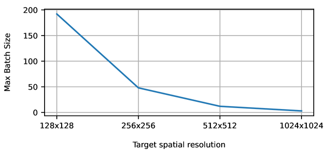
Figure 1: Maximum allowable batch size during inference at different target spatial resolutions for SOTA DL super-resolution methods [16] on a 16GB NVIDIA V100 GPU with 16-bit floating point precision.

Spatially uniform outputs are computationally inefficient for two other reasons. First, they can under-resolve areas with complex flow features and over-resolve regions with smooth fluctuations in the flow properties. It is critical to capture this versatility for complex systems with large variations in their local solutions, such as turbulent flows. Second, current uniform super-resolution approaches need to know the target resolution a priori. As a result, they require a large number of HR labels at that specific resolution. They hence need to rely either on publicly available datasets or on performing data collection. Since the resolutions of the publicly available datasets are very limited, the majority of works [13, 15, 18, 19] end up performing computationally challenging high-resolution data collection.

Due to the large scale of many applications, it is often infeasible to solve the problem on a uniform mesh to achieve the desired accuracy. For this reason, traditional numerical solvers do not refine the entire mesh but do so adaptively, refining only regions of strong flow variability for scalability and performance - a method commonly referred to as Adaptive Mesh Refinement (AMR) [20, 21]. However, traditional AMR methods in CFD suffer from two fundamental limitations. First, a high degree of user intervention in the refining/coarsening decisions: these decisions are based on heuristics that require problem-specific knowledge and do not generalize well. Second, the mesh is refined iteratively, requiring more compute time and memory compared to direct methods.

In this paper, we tackle all these challenges and present NUNet, a novel DL framework for Non-Uniform super-resolution. NUNet takes as input a LR flow field and outputs, in one-shot, its final non-uniform HR solution, as seen in Figure 2. Since only regions in areas that present complex flow phenomena are refined, it requires less computational resources. This enables larger batch sizes during inference at high spatial resolutions while reaching the target accuracy compared to SOTA methods for super-resolution. NUNet distinguishes between different regions of the domain by dividing the input LR flow field into fixed-size patches, adaptively increasing or maintaining the spatial resolution of each patch, and predicting a non-uniform HR flow field. We present NUNet as an end-to-end DL-physics solver framework where the non-uniform output field from the model inference is input to a traditional physics solver that drives the solution to convergence. As a result, NUNet meets the same convergence guarantees as AMR solvers which is critical for practitioners [22, 16, 23].

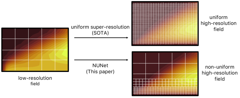
Figure 2: Current DL algorithms for super-resolution output the solution on a uniform fine mesh (top). Our objective with NUNet is to predict a spatially non-uniform output where only areas that require higher accuracy are refined (bottom). Hence, NUNet requires less compute time and memory resources while achieving the target accuracy.

Specifically, NUNet makes the following contributions:

• Non-uniform super-resolution. To enable non-uniform super-resolution, we propose a novel scorer-ranker-decoder DL algorithm, where the scorer finds the spatial score of each patch, the ranker places each patch in its corresponding bin based on its score (which determines the target resolution of a patch), and the decoder reconstructs every patch in each bin to its final target resolution using semi-supervised learning.

• Requires minimal user intervention. NUNet’s training is semi-supervised - the loss function that guides its optimization process is formed by the governing equations of the problem - which poses a two-fold advantage. First, the refinement or coarsening decisions are based on physics principles with the least possible human intervention, as opposed to traditional AMR solvers that require expert, domain, and even problem-specific knowledge and a high degree of user intervention [21]. From one single training, NUNet reaches SOTA refining/coarsening decisions for different flow problems that exhibit very different flow phenomena, showcasing remarkable generalization properties. Second, NUNet does not require to know the target resolution a priori and hence eliminates the need of expensive high-resolution data collection.

• Outperforms traditional AMR solvers. We evaluate NUNet on three canonical turbulent flows obtained from Reynolds-Averaged Navier-Stokes (RANS) simulations on seven flow configurations unseen during training – three unseen geometries and four unseen boundary conditions. NUNet’s adaptively refined meshes show excellent flow discerning properties and agreement with the baseline OpenFOAM AMR solver in refining regions of interest such as near-wall areas in wall-bounded problems (channel flow, flat plate), in flow around smooth solid bodies (flow around an airfoil), and the wake region in flow around thick solid bodies (flow around a cylinder) while maintaining less complex flow areas, such as the freestream, at low resolution. NUNet predicts the non-uniformly refined final flow field in a single inference step as opposed to traditional AMR solvers that require several iterations. As a result, NUNet reaches the same convergence guarantees as the AMR solver while accelerating it by $3.2-5.5\times$.

• Requires less computational resources. Due to NUNet’s ability to only refine specific areas of the flow and avoid high-resolution inferences in the entire the domain, it achieves a speedup of $7-28.5\times$ and reduces the memory usage by $4.4-7.65\times$ at $1024\times 1024$ spatial resolutions compared to SOTA DL methods that perform uniform super-resolution while reaching SOTA accuracies.

2 Related Work

Adaptive Mesh Refinement (AMR). AMR is a popular technique that makes it feasible to solve problems that are intractable on uniform grids and it has been widely applied in traditional finite volume-based solvers. When PDEs are solved numerically, they are often limited to a pre-determined computational grid or mesh. However, different areas of the domain can require different precisions where non-uniform grids are better suited. AMR algorithms adaptively and dynamically identify regions that require finer resolution (such as discontinuities, steep gradients, and shocks) and refine or coarsen the mesh to achieve the target accuracy. Therefore, AMR can scale to resolutions that would otherwise be infeasible on uniform meshes resulting in increased computational efficiency and storage savings. Moreover, the adaptive strategy offers more control over the grid resolution compared to the fixed resolution of the static grid approaches. The most popular AMR techniques apply to traditional finite volume/finite element based numerical solvers. Even though recent approaches have notably pushed the scalability boundaries of these systems [10, 21, 20] their core strategy results from the early work of  Berger and Oliger [24], who introduced local adaptive mesh refinement. This algorithm starts with a coarse mesh from which certain cells are marked for refinement according to either a user-supplied criterion or based on the Richardson extrapolation [25]. The principle of marking cells for refinement is widespread. Two main approaches exist for identifying cells for refinement. First, adjoint-based AMR [26], which estimates the discretization error in each cell and adapts the mesh for lowering these errors. However, the optimal rationale for error estimation remains unknown [27]. Second, feature-based AMR [28], where the user supplies the variables (or features) to track and refines the computational cells that meet a user-defined value of those variables. Feature-based AMR is the most popular approach due to less challenging implementations and accurate results in a wide range of problems. However, feature-based AMR approaches require both a high degree of user intervention and expert, domain, and even specific knowledge of the problem at hand, and therefore have poor generalization properties. Existing AMR methods are based on a handful of heuristics whose long-term or general optimality remains unknown. To overcome this limitation,  Yang et al. [29] designed the AMR procedure as a Markov Decision Process. However, the training is done with ground truth data generated from analytical solutions and can not be extended to turbulent flows.

There have been recent attempts to perform DL-based AMR. In [30], the authors increase the number of solution points in those areas where the residual is highest. However, this mesh-free method imposes the same refinement heuristics as traditional physical solvers and hence suffers from the same limitations. In [31], the authors develop AMRNet, a CNN-based model that performs multi-resolution, where the network outputs a uniform flow field at different resolutions. Since the output is uniform there is no discrimination between different areas of the flow. As opposed to the above approaches, we design a DL algorithm for AMR, where the output is non-uniform and we do not impose any heuristic during the optimization process of the network. Instead, the training is guided by the governing equations of the problem that inform refining decisions (described in Section 3.2).

Super-resolution. DL algorithms have shown impressive results for super-resolution. We find super-resolution techniques applied to both CV and CFD problems. Two main research directions exist in CV: single-image super-resolution (SISR) and reference-based super-resolution (RefSR). However, both SISR and RefSR have a target resolution that is both known a priori and uniform [32, 33, 34]. In [34], the authors present the texture transformer, where the query, key, and value of their attention module are formed by upsampled and downsampled images of the input image together with a reference image from which textures are extracted. In [35], the authors provide a differentiable module that selects the most salient patches of the input image for image classification. However, the unselected patches are unused. In this paper, we are interested in super-resolution, and therefore we keep all patches that cover the entire domain.

In CFD, we also find successful super-resolution attempts. Recent works use CNNs as finite-dimensional maps  [17, 15, 19]. However, these approaches know the target resolution a priori, perform uniform SR, and require large amounts of HR labels. To eliminate the need for large amounts of HR labels, authors in [16] developed SURFNet, a transfer learning-based uniform SR framework. This work reduces the HR data requirement by $15\times$ while achieving resolution invariance. However, it’s also limited to uniform SR. Mesh-free, resolution-invariant methods [13, 36, 37, 18, 38] are a potential alternative to finite-dimensional maps because they can query the solution at any point in the domain and hence are prone to perform non-uniform SR. In [13], the authors developed MeshFreeFlowNet, an efficient framework for super-resolution of turbulent flows that demonstrates improved accuracy compared to baseline models [39].  Lu et al. introduced a neural operator, which provides a set of network parameters compatible with different discretizations and hence exhibits resolution-invariance – achieving constant accuracy across discretizations. However, this class of methods do not intrinsically discriminate between different regions of the flow and hence end up yielding uniform output resolutions. Moreover, they also suffer from the limitation of extensive HR data collection.

In this paper, we present a semi-supervised DL algorithm that adaptively refines the input mesh and outputs a non-uniform HR flow field, improving both inference times and memory requirements for scaling to large problem sizes. NUNet does not require knowledge of the target resoluton a priori, hence eliminates both the need for collecting extensive HR training data and the dependence on existing datasets that are limited to specific resolutions.

3 NUNet: DL for AMR

Our objective is three-fold. First, to predict fine-grid turbulent flows from their coarse-grid counterpart only in the regions of interest. Second, to design a DL algorithm for AMR where these areas to refine are identified with the least possible user intervention. Third, to output a solution that meets the same convergence guarantees as classical AMR solvers.

In this section, we present NUNet, a novel DL framework for adaptive super-resolution. We first describe in detail the neural network architecture and then, present our semi-supervised learning approach that leverages a hybrid loss function. Finally, we outline the end-to-end framework, which reconstructs a non-uniform HR flow field while reaching the same convergence as the state-of-the-art AMR solvers.

3.1 Neural Network Architecture

We choose a deep neural network (DNN) for the task of non-uniform super-resolution. The input to the DNN is a low-resolution flow field, which is divided into fixed-size regions or patches. The output is a non-uniform resolution flow field, where high-resolution is given only at specific patches of the domain. The RANS equations with the Spalart-Allmaras model (described in Section 4.1) predict four main flow variables – mean x-velocity ($U$), mean y-velocity ($V$), the mean kinematic pressure ($p$), and the eddy viscosity ($\tilde{\nu}$). Therefore, the input LR flow field consists of a four-channel tensor image where each channel represents the values of one flow variable in the entire computational grid. The DNN scores, ranks (or bins), and predicts the target resolution of each patch. Figure 3 illustrates the architecture composed of a scorer network, a ranker, and a decoder network.

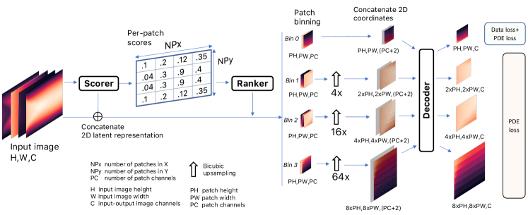
Figure 3: NUNet’s DNN. The input is a four-channel LR image where each channel represents one flow variable. The LR image is first input to the scorer, which divides it into patches and outputs the score of each patch. The ranker uses these scores to assign each patch to a bin, which is subsequently upsampled using a bicubic interpolation to its target resolution. Then, the upsampled patches are concatenated with their coordinates. Finally, the decoder maps this upsampled, intermediate representation to the final values of each patch. NUNet’s DNN’s output is multiple, consisting of a list of four-channel images at different spatial resolutions.

Scorer. The LR flow field is first input to the scorer network. This is a trainable network whose goal is to score each patch of the LR image via its 2D spatial latent representation, as illustrated in Figure 4. This network is inspired by the work of  Cordonnier et al. [35] that use a similar network for finding salient patches from the input image for classification.

Figure 4: The scorer network. It consists of four convolutional layers followed by maxpool and softmax layers. The first three convolutional layers extract a single-channel 2D latent spatial representation from the input LR flow field. This 2D latent representation is used to obtain the scores of each patch via a maxpooling and a softmax layer. It is also output and concatenated with the original LR image.

The scorer network consists of a shallow CNN followed by a maxpooling layer and a softmax layer. The first three convolutional layers extract an abstract representation of the LR flow field. Their kernel size is $(5,5)$ and the stride is 1. This overlap captures the spatial relationships between and among the input flow variables – a $(5,5)$ kernel can capture both short and long-range dependencies and a stride of 1 maintains the spatial dimensionality. After the first three convolutional layers, we apply a single-filter convolutional layer to squeeze and encapsulate the extracted abstract spatial information in a single-channel image. This image is a 2D latent representation of the spatial dependencies in the variables of the LR flow field and plays a key role in determining the scores of each patch. This single-channel image is input to the maxpooling layer that splits the domain into ${NP}_{x}\times{NP}_{y}=N$ patches – where ${NP}_{x}$ is the number of patches in the horizontal direction, ${NP}_{y}$ is the number of patches in the vertical direction, and $N$ is the total number of patches. The pool size and the stride are both $(ph,pw)$, where $ph$ is the height of the patch and $pw$ is the width of the patch. Hence, each value in this image represents the non-normalized score of each patch. The softmax layer normalizes these scores to a $0-1$ scaled probability distribution. The scorer network’s output is twofold: the scaled scores and the 2D latent representation.

Before passing the scores to the ranker, we concatenate the 2D spatial latent representation with the LR flow field. This is motivated by two reasons. First, the latent representation already contains spatial correlations from the LR flow field. Second, it allows to dynamically change the scores of the patches since the scorer’s weights are propagated during the backward pass of the training process. Hence, the LR flow field becomes a five-channel image (in Figure 3, $PC=5$). Finally, we pass the scores from the scorer to the ranker.

Ranker. This is a non-trainable module that tracks the score and the ID of each patch. The ranker locates each patch in the new five-channel LR flow field, isolates it from the rest of the image, and places it in a bin according to its score. We refer to this process as binning, and it is illustrated in Figure 3. Binning consists of splitting the $0-1$ range of values of the scores into $b$ bins uniformly. For instance, if $b=2$, the first bin consists of patches with scores between $0-0.5$, and the second bin with scores $0.5-1$. The ranker plays a significant role in determining the final resolution of each patch: training consists of mapping the highest-scored patches to the highest target resolution, and as scores gradually decrease, so does the target resolution of the patch. The patches with the lowest scores remain low-resolution.

After the binning finishes, we perform two additional steps before passing the patches to the decoder. First, we upsample (refine) each patch to its target resolution using bicubic interpolation, as seen in Figure 3. Then, we concatenate the 2D coordinates to each patch needed to compute the gradients of the flow variables using automatic differentiation [40]. This leads to a seven-channel image (in Figure 3, $PC+2$). Once we upsample and concatenate the coordinates to the patches, it is input to the decoder.

Decoder. The goal of this trainable network illustrated in Figure 5 is to reconstruct the high-resolution solution of each patch. Each patch in each bin passes through the same decoder, which is shared among resolutions. Note that the patches placed in the low-resolution bin also passes through the decoder. The choice of a shared decoder is motivated by two reasons. First, we have a smaller number of learnable parameters compared to a separate decoder for each resolution. Thus, we stress NUNet’s ability to recover different resolutions for different patches with a lower computational cost. Second, the low-resolution patches have not been upsampled and the decoder can extract the true spatial correlations between the flow variables and coordinates in those patches. We expect this to help in recovering the true values of the high-resolution patches.

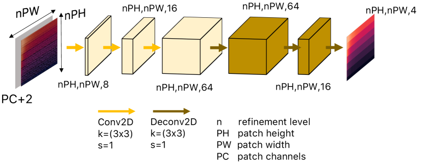
Figure 5: The decoder network. The input to the decoder is the intermediate patch representation concatenated with the 2D coordinates at its target resolution. This network consists of 3 convolutional layers followed by 3 deconvolutional layers that reconstruct the final values of the patch at its target resolution. The output is, therefore, a four-channel image, where each channel is the value of a flow variable.

This network is a 6-layer network; 3 convolutional layers followed by 3 deconvolutional layers. The number of filters is 8, 16, 64, 64, 16, 4; the kernel size is $(3,3)$, and the stride is 1. The choice of this architecture is twofold. First, recent works have successfully leveraged similar architectures for flow super-resolution [14, 16]. Second, the convolutional layers aim at extracting a deep, abstract representation used by the deconvolution layers to reconstruct the high-resolution output. We use a stride of 1 to not lose any spatial information.

The decoder’s output consists of a list of patches. Each patch is a four-channel image, and each channel represents the values of the four flow variables ($U$, $V$, $p$, and $\tilde{\nu}$) at steady-state at their new spatial resolution. Each patch in the list can have a different spatial resolution. This list is then passed to the loss function.

3.2 Loss function

Recent DL-based super-resolution approaches have leveraged data-only loss functions [16, 15], where CFD simulations generate the ground truth labels. Other approaches use a combination of data and PDE residual loss function [13, 14], where the governing equations are imposed in the loss function. We adhere to the latter practice for a couple of reasons. First, it is physically and numerically inconsistent to merge CFD-originated data from different spatial resolutions. Second, we do not train with ground truth data from AMR solvers because that would make the network learn the solver’s heuristics that have a high degree of user intervention. The goal is for NUNet to make its own refining decisions to obtain a DL-based model for AMR. Equation 1 shows our loss function.

$$\mathbb{L}=\frac{1}{np\cdot nc\cdot fv}\sum_{i=1}^{np}\sum_{j=1}^{nc}\sum_{k=1}^{fv}\left\lVert\hat{y}_{ijk}-y_{ijk}\right\rVert^{2}+\frac{\lambda}{NC\cdot ne}\sum_{i=1}^{NC}\sum_{j=1}^{ne}\left\lVert P_{j}(i)\right\rVert^{2}$$ (1)

Our loss function $\mathbb{L}$ is formed by two parts. The first term in the right hand side of Equation 1 is the data loss. We take the mean squared error (MSE) of the prediction of each flow variable ($fv$) at each cell ($nc$) of the low-resolution patches ($np$) only with the ground truth data obtained with the physics solver. The second term in the right hand side is the L2 norm of the residual of each PDE ($ne$) for all cells ($NC$) of the output image, belonging to either low or high resolution patches. We impose the continuity equation and the two conservation of momentum equations (hence, $ne=3$), described in Equations (2) and (3). The gradients of the variables are computed through automatic differentiation [40]. To constrain the PDE residual of the high-resolution patches, we downsample them using bicubic interpolation to the lowest resolution and match the ground truth data in the downsampled space [14]. With this semi-supervised learning formulation, we avoid HR labels, an advantage over SOTA super-resolution methods that require expensive HR training data [13, 37, 18, 38].

3.3 End-to-end framework

Once the network is trained and calibrated, we use it to predict the non-uniform high-resolution flow field of a new problem. However, this prediction has an approximation error and might not satisfy the same convergence constraints as traditional physics solvers with PDE residual values close to the machine round-off errors, which is critical for many practitioners. We correct this by refining the DNN’s prediction using the physics solver [23, 22, 16].

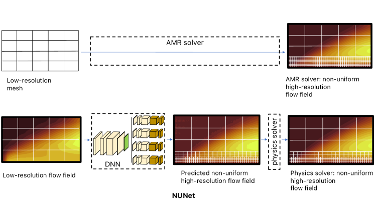
Figure 6: Top: Traditional AMR solver simulation. Bottom: NUNet framework. After performing non-uniform super-resolution with the DNN, we feed the output field into the physics solver, which takes the inferred solution to convergence.

Figure 6 illustrates NUNet’s end-to-end framework compared with the traditional AMR solver. In NUNet, the LR flow field is input to a DNN, whose architecture is detailed in Section 3.1. After inference, we feed the DNN’s non-uniform output into the physics solver, impose the boundary conditions that well-pose the problem, and let the physics solver drive this inference to convergence. Note that the physics solver does not do any further refinement or coarsening. The final discretization is an output of the DNN.

As a result, we obtain a solution that satisfies the same convergence constraints as traditional numerical methods. Since we anticipate the DNN’s inference to be "close" to the final solution, convergence is accelerated. Section 5.1 empirically evaluates the performance of NUNet against both classical AMR solvers and SOTA DL models.

4 Experiment Setup

In this section, we present the methodology to train and evaluate NUNet. We first describe the governing equations then, present the dataset to train and validate NUNet along with the training/testing setup, parameters, and results. Finally, we describe the physics solver and the traditional AMR heuristics used for comparison.

4.1 Background

We use steady incompressible Reynolds-Averaged Navier-Stokes problems for our non-uniform super-resolution task. The RANS equations describe turbulent flows as follows:

$$\frac{\partial\bar{U}_{i}}{\partial x_{i}} =0$$ (2)

$$\bar{U}_{j}\frac{\partial\bar{U}_{i}}{\partial x_{j}} =\frac{\partial}{\partial x_{j}}\left[-\left(\bar{p}\right)\delta_{ij}+\left(\nu+\nu_{t}\right)\left(\frac{\partial\bar{U}_{i}}{\partial x_{j}}+\frac{\partial\bar{U}_{j}}{\partial x_{i}}\right)\right]$$ (3)

where $\bar{U}$ is the mean velocity, $\bar{p}$ is the kinematic mean pressure, $\nu$ is the fluid laminar viscosity, and $\nu_{t}$ is the eddy viscosity. Equation 3 is a vector equation that yields two scalar equations - one for each spatial direction. The RANS equations are a time-averaged solution to the incompressible Navier-Stokes equations but result in a non-closed equation. We close the equation with Boussinesq’s approximation [1] by relating the Reynolds stresses with the mean flow: we model the Reynolds stresses with the eddy viscosity and the main rate of the strain tensor. We then model the eddy visccosity with the Spalart-Allmaras (SA) one-equation model, that provides a transport equation to compute the eddy viscosity [41], described in Equation 4

$$\bar{U}_{i}\frac{\partial\tilde{\nu}}{\partial x_{i}}=C_{b1}\left(1-f_{t2}\right)\tilde{S}\tilde{\nu}-\left[C_{w1}f_{w}-\frac{C_{b1}}{\kappa^{2}}f_{t2}\right]\left(\frac{\tilde{\nu}}{d}^{2}\right)\\ +\frac{1}{\sigma}\left[\frac{\partial}{\partial x_{i}}\left(\left(\nu+\tilde{\nu}\right)\frac{\partial\tilde{\nu}}{\partial x_{i}}\right)+C_{b2}\frac{\partial\tilde{\nu}}{\partial x_{j}}\frac{\partial\tilde{\nu}}{\partial x_{j}}\right]$$ (4)

From Equation 4 we can compute the eddy viscosity from $\tilde{\nu}$ as $\nu_{t}=\tilde{\nu}f_{v1}$. These equations represent the most popular implementation of the Spalart-Allmaras model. The terms $f_{v1}$, $\tilde{S}$, and $f_{t2}$ are model-specific and contain, for instance, first order flow features (magnitude of the vorticity). $C_{b1}$, $C_{w1}$, $C_{b2}$, $\kappa$, and $\sigma$ are constants specific to the model, found experimentally. $d$ is the closest distance to a solid surface. We choose the RANS equations with the Spalart-Allmaras turbulence model because (1) it is a one-equation model and, therefore, computationally convenient, and (2) it has been widely explored in all our benchmark cases (see Section 4.2), including aerospace applications for which SA was designed. If we can mimic the AMR behavior with SA, we are optimistic that our approach can be applied to many RANS turbulence models. The constants of the model are those in its original reference [41].

4.2 Dataset Overview and Flow Description

We gather low-resolution data from three well-known canonical flows for training the DNN in Figure 3. The resolution for this dataset is $64\times 256$, since it is a common resolution for low-resolution solutions for all our training cases [1].

Turbulent flow in a channel. 2D channel flow has been widely studied in the literature [42]. A common strategy to evaluate channel flow is to vary the input velocity to the channel. This is the same as varying the Reynolds number since Re $=\frac{UL}{\nu}$, where $U$ is the input velocity to the channel, $L$ is the diameter of the channel, and $\nu$ is the laminar viscosity of the problem. Here, we adhere to this practice and vary the input velocity to the channel to collect $10000$ samples. Specifically, we collect 300 samples from Re = $2103$ (when turbulent effects start to appear [1]) to Re = $2.3103$, and then, 9700 more samples from Re = $2.7103$ to Re = $1.35104$. We leave Re = $2.5103$ and Re = 1.5e4 as our test cases. Section 5 presents a more in-depth discussion of the selection of the test cases. The physical domain of the channel flow is a diameter of 0.1 meters and a length of 6 meters so we find fully developed flow. The inlet is at the left and the outlet at the right. The top and the bottom are both walls and hence have the no-slip boundary condition. The velocity boundary conditions are uniform inlet at the inlet, no-gradient at the outlet, and 0 at the walls. The pressure boundary conditions are no-gradient at the inlet, 0 uniform at the outlet, and no-gradient at the walls. The modified eddy viscosity boundary conditions are $3\times$(laminar viscosity) at the inlet, no-gradient at the outlet, and 0 at the walls. The laminar viscosity is set to $110-4$ $\mathrm{m}^{2}\mathrm{/}\mathrm{s}$ .

Turbulent flow over a flat plate. Flat plate is also a canonical flow, part of the wall-bounded flows family, used to study the boundary layer in both laminar and turbulent conditions [1]. By varying the incoming velocity we collect 10000 samples. For flat plate, incompressible turbulent effects do not appear [1] up until Re = $1.35105$ and scale up to Re = $5106$. We collect 2000 samples from Re = $1.35105$ to Re = $2105$ and another 8000 additional samples from Re = 3e5 until Re = 1.1e6. We leave Re = $2.5105$ and Re = $1.35106$ as test cases. The physical domain of the flat plate case is a height of 0.2 meters and a length of 10 meters, as found in different benchmarks. The boundaries are a wall at the bottom (the flat plate), symmetry at the top, an inlet at the left, and an outlet at the right. The velocity boundary conditions are uniform inlet at the inlet, no-slip condition at the bottom wall, no-gradient both at the outlet. The pressure boundary condition is no-gradient at the inlet and bottom wall, and 0 at the outlet. The modified eddy viscosity boundary conditions are $3\times$(laminar viscosity) at the inlet, 0 at the bottom wall, and no-gradient at the outlet. The laminar viscosity is set to $110-4$ $\mathrm{m}^{2}\mathrm{/}\mathrm{s}$.

Turbulent flow around ellipses. External aerodynamics simulations are relevant for aerospace industrial applications. We gather low-resolution solutions from flow around ellipses. In real scenarios, different geometries at a variety of flow conditions are explored. Our training data consists of 10000 samples of flow around different ellipses at different flow conditions. Figure 7 shows these configurations.

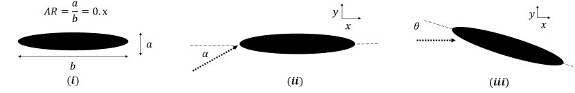
Figure 7: Sketch of the (i) ellipse aspect ratio, (ii) angle of attack $\alpha$, and (iii) pitch angle $\theta$.

The training data is obtained by changing the aspect ratio of the ellipses: $0.05,0.07,0.09,0.1,0.15,0.2,0.25,0.35,0.55$, and $0.75$. Each of these ellipses is simulated under 5 different flow conditions by changing randomly the angle of attack $\alpha$ and the pitching angle $\theta$ between $-2$ and $6$ degrees. We collect all of these configurations at 200 different Re numbers between $5104$ and $9104$. We select flow around a cylinder at Re = $1105$, flow around a symmetric airfoil (NACA0012) at Re = $2.5104$, and flow around a non-symmetric airfoil (NACA1412) at Re = $2.5104$. The physical domain of the ellipse/cylinder/airfoil cases consists of a solid body of chord ( c ) 1 meter, and the far-field limit is located 30c from the tip and tail of the solid body (O-grid type of mesh). The velocity boundary conditions are no-slip at the wall and uniform velocity at the far-field; the pressure boundary conditions are no-gradient at the wall and uniform 0 in the far-field; the modified eddy viscosity boundary conditions are 0 at the wall and uniform $3\times$(laminar viscosity) in the far-field, where the laminar viscosity is $110-4$ $\mathrm{m}^{2}\mathrm{/}\mathrm{s}$ uniform in the entire domain.

The total training set size is composed of $30000$ samples, $10000$ from each canonical flow. From this training dataset, $27000$ samples are used for training the DNN and $3000$ samples are used for validation.

4.3 Training and Testing Setup

The methodology described in Section 3 allows for multiple combinations of parameters in addition to those in neural network optimization. For instance, we can select different patch sizes or different number of bins (and therefore, different number of target resolutions). In this section, we explain our training design choices.

First, NUNet’s DNN’s convolutional kernels of size $5\times 5$ and $3\times 3$ require a minimum input image size to extract relevant information. Therefore, we fix our patch sizes at $ph\times pw=16\times 16$, which leads to $N=64$ total number of patches for each train/validation/test sample. Larger patch sizes (for instance, $32\times 32$) do not offer enough granularity to make critical distinctions between regions of the flow. Second, we choose the number of bins $b=4$, and hence four different target resolutions. Each target resolution refines the original low-resolution patch by $4^{(n)}\times$, where $n=0,1,2,3$. We choose $b=4$ because not more than 4 levels of refinement is an extended practice in the AMR literature [24, 28] to avoid tiny computational cells. This also allows us to compare NUNet with SOTA approaches that attempt $64\times$ super-resolutions. The patch size and the number of bins are the same at test time and during the evaluation of the results.

We implement the DNN using the Tensorflow 2.4 backend, and perform distributed training on four Tesla V100 GPUs connected with PCIe. After training the network with a batch size of $8$, a learning rate of $1e-4$, no specific initialization, and using the Adam optimizer [43] for 350 epochs, the training and validation data and PDE residual loss for all equations reach a MSE of 9e-6. Note that the training of NUNet’s DNN is done on the Tesla V100 GPUs. However, NUNet is implemented entirely on the CPU for a fair comparison with the AMR solver, which only supports CPU. Hence, both NUNet and the AMR solver are executed on the CPU.

4.4 Physics solver and AMR solver

Once the network is calibrated, it is used for inference. Recall that the DNN’s output is input into the physics solver to drive the flow field from inference to convergence (see Section 3.3). We use OpenFOAM’s pimpleFoam [3, 44] solver as the physics solver in this paper. For the pressure, we use the GAMG solver, with a relative tolerance of 0.1, and the GaussSeidel smoother from OpenFOAM. For the velocity and the eddy viscosity, we use the smoothSolver with a relative tolerance of 0.1. The number of outer and inner correctors are set to 1, and the time scheme is set to steady-state.

As for the AMR solver to compare NUNet with, we use the dynamicMeshRefine utility in OpenFOAM. This utility performs AMR as long as it is used together with pimpleFoam solver. The combination of the pimpleFoam solver with the
dynamicMeshRefine utility forms the AMR solver used in this paper. This solver is a feature-based AMR solver, which is the most popular method in the literature [21]. Therefore, it requires user intervention: for all of the test cases, we set the AMR solver to refine those areas where the gradients of the eddy viscosity are the highest, and the maximum level of refinement is set to 4. This heuristic is popular and works well for a wide range of problems, including our test problems [1].

Architecture and Libraries. All the OpenFOAM simulations are run in parallel on a dual-socket Intel Xeon Gold 6148 using double precision due to the lack of GPU support. Each socket has 20 cores, for a total of 40 cores. We use the OpenMPI implementation of MPI integrated with OpenFOAM v8 that is optimized for shared-memory communication. The grid domain is decomposed into 40 partitions using the integrated Scotch partitioner and each partition is assigned to 1 MPI process that is pinned to a single core. We set the numactl -localalloc flag to bind each MPI process to its local memory.

5 Results and Discussion

After training and validating the network, we evaluate NUNet’s ability for non-uniform super-resolution on two different use cases, as outlined below:

1. Same geometry, different boundary conditions. We use NUNet to refine the LR solution of flow on a geometry observed during training but at a different boundary condition. Here, our test flows configurations are channel flow and flat plate on interpolated (int) and extrapolated (ext) boundary conditions. For the former, we test on Re = $2.5103$ (int) and Re = $15103$ (ext). For the latter, we test on Re = $2.5105$ (int) and Re = $1.35106$ (ext).

2. Different geometry, different boundary conditions. We stress the generalization capacity of NUNet by finding the non-uniform high-resolution solution of flow around geometries unseen during training. We use the same network to predict the flow around a cylinder at Re = $1105$, the flow around a symmetric NACA0012 [7] airfoil atRe = $2.5104$, and the non-symmetric NACA1412 airfoil at Re = $2.5104$, as seen in Figure 8.

For the described test cases, we first present the accuracy and correctness of NUNet by comparing it, both qualitatively and quantitatively, with the traditional AMR solver (described in Section 4.4). Then, we present the performance analysis of NUNet by showing (1) its speedup over the AMR solver and (2) the improved inference time and memory usage over the SOTA neural network models that perform uniform super-resolution. The baseline neural network used for comparison is described in Section 5.2.

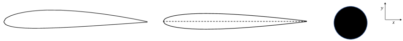
Figure 8: Non-symmetric NACA1412 airfoil (left), symmetric NACA0012 airfoil (center), and cylinder (right) as test geometries. These test cases stress the generalization capacity of NUNet on unseen-during-training geometries.

5.1 Correctness and Accuracy of NUNet

Once the DNN is trained, we build the NUNet framework and study its correctness and accuracy by comparing it with the traditional AMR solver. We first conduct a qualitative evaluation by visualizing (a) the refined/unrefined areas and (b) the final flow field by the two algorithms. Because of the difference in their inherent heuristics (NUNet follows an optimization process containing different flow cases while the AMR solver follows user-given heuristics as explained in Section 4.4), we do not expect the exact same output. However, the qualitative results evaluate whether NUNet can act as an AMR surrogate for multiple flow problems resulting from a single training.

After, we present a quantitative comparison between the two using a grid convergence study [45]. Recall that both NUNet and the AMR solver solve the same problem. We impose the same strong-form boundary conditions in the fluid domain, which well-pose the problem and guarantee uniqueness [46]. The only metric that changes between the two is the mesh, and therefore, they will present different discretization errors. However, these discretization errors reduce as we increase the resolution of refinement and global quantities tend to converged solutions [1]. Hence, to evaluate the quality of NUNet’s inferred mesh, we compare the solution from both NUNet’s mesh and the AMR solver mesh as we increase the required levels of refinement. Both meshes are refined $4^{n}\times$ gradually, from $n=0$ to $n=3$. Then, we report the value of specific quantities of interest (QoI) at steady-state. The choice of the QoI follows the CFD literature [1].

5.1.1 Qualitative Results

Figure 9 shows the refined/unrefined results for five test cases: channel flow at Re = $2.5103$, flat plate at Re = $1.35106$, cylinder, and the two airfoil test cases. Figure 9 shows NUNet’s predicted mesh (left) and the AMR solver’s output mesh (right). NUNet splits the domain into 64 $16\times 16$ patches and we show the output resolution (with respect to the coarse resolution) of each patch. Because the AMR solver allows more granularity as it performs mesh refinement on a per-cell basis, the domain is divided into smaller ($4\times 8$) patches. At the borders of each test case, we show the physical boundaries of each case which play a key role in determining the areas where both algorithms refine the mesh.

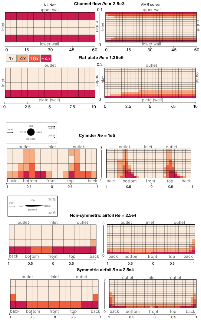
Figure 9: Per-patch fluid domain and the level of refinement of each patch for all our test cases. First row: channel flow at Re = $2.5103$. Second row: flat plate at Re = $1.35106$. Third row: cylinder at Re = $1105$. Fourth row: non-symmetric NACA1412 airfoil at Re = $2.5104$. Fifth row: symmetric NACA0012 airfoil at Re = $2.5104$. We compare NUNet’s prediction (left) versus AMR solver’s output (right). Both axes are in meters.

We make three main observations. First, NUNet can distinguish between boundary conditions. For the channel flow case (first row in Figure 9), NUNet refines the fluid areas close to both the upper and the lower wall, whereas, for the flat plate case (second row), it refines the areas close to the wall but leaves the outer regions (outlet/freestream) at low resolution. Second, NUNet respects the symmetry of the problem, as we observe in the channel flow case (first row of Figure 9) and in the symmetric airfoil case (fifth row in Figure 9). Third, NUNet’s fine/coarse regions are in excellent agreement with those of the AMR solver for the channel flow, flat plate, and airfoil cases. This agreement in the cylinder case is also notable. For instance, NUNet refines the region of the flow from the back of the cylinder to the outlet (i.e., the wake behind the cylinder). However, we observe some discrepancy in the back-bottom-front-top region. The front-bottom-back and front-top-back regions (which refer to the entire solid boundary of the cylinder) require a higher resolution from NUNet. This difference, together with the channel flow and flat plate results, indicates that the DNN is refining those areas with higher values of the gradients for all fluid variables, which take place in solid wall boundaries [1]. This is opposed to the AMR solver’s heuristic, that focuses only on areas with high gradients of the eddy viscosity.

During the calibration of the DNN, it is key to balance both components of the loss function - the data loss and the PDE residual loss (described in Section 3.2) so neither dominates the other. In our experiments, we observe the best predictive results at $\lambda=0.03$, which yields a balanced contribution of each component of the loss. The data and PDE residual loss reached a value of $910-6$ for both the training and the validation samples. During training, we scale the value of the variables between 0 and 1 for learning stability purposes. However, we can not scale the value of the gradients found by automatic differentiation because this would result in inconsistent PDE residual loss. These gradients reach higher absolute values than those of the data, especially in areas of the flow with higher variability, and hence get the attention of the MSE loss function. Moreover, this also allows NUNet to refine the back-outlet area, where the wake region of the flow after the cylinder meets the freestream (outlet) and we find a high gradient of the eddy viscosity. The difference in the refining patterns between the cylinder and the airfoil case is that the former presents flow separation from the wall boundary that generates a wide wake region, whereas in the airfoil case the flow remains attached to the solid.

Figure 9 also shows that in the channel flow, flat plate, and airfoil test cases, the AMR solver reduces the refinement level gradually as we increase the distance from the wall boundary. Instead, NUNet infers the maximum level of refinement in the patches close to the wall and does not show this gradual reduction. This is due to the maxpooling layer in the design of NUNet’s scorer network (see Section 3.1). Recall that the maxpooling layer chooses the highest score present in the $16\times 16$ region defined by the patch. Choosing a maxpooling layer over an average pooling is a desired conservative approach. Since an entire patch shares a resolution in NUNet, it is advantageous to choose the highest required resolution even if only few cells within a patch require it for accuracy. Figure 9 shows that NUNet and the AMR solver have inherently different heuristics for mesh refinement/coarsening and do not produce the same mesh - as expected. However, both are in excellent agreement in their steady flow field prediction, as we qualitatively observe in Figures 10, 11, 12,  13, and 14.

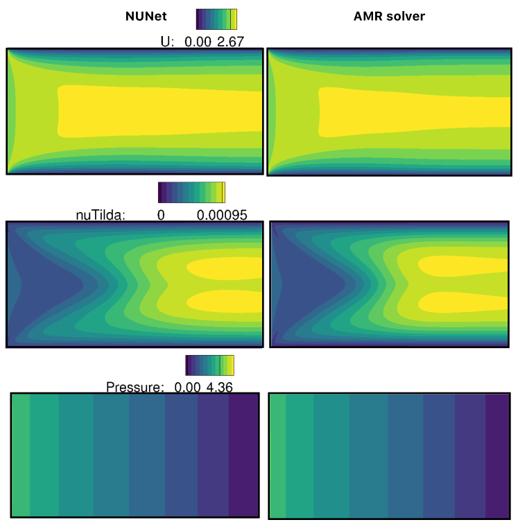
Figure 10: Channel flow at Re = $2.5103$. Velocity in $\mathrm{m}\text{\,}{\mathrm{s}}^{-1}$ (top), kinematic pressure in $\mathrm{m}^{2}\mathrm{/}\mathrm{s}^{2}$ (bottom), and modified eddy viscosity in $\mathrm{m}^{2}\mathrm{/}\mathrm{s}$ (middle). Comparison between NUNet’s result (left) and the AMR solver result (right) for $b=4$ levels of refinement.

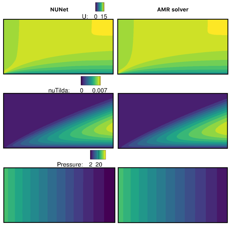
Figure 11: Flat plate at Re = $1.35106$. Velocity in $\mathrm{m}\text{\,}{\mathrm{s}}^{-1}$ (top), kinematic pressure in $\mathrm{m}^{2}\mathrm{/}\mathrm{s}^{2}$ (bottom), and modified eddy viscosity in $\mathrm{m}^{2}\mathrm{/}\mathrm{s}$ (middle). Comparison between NUNet’s result (left) and the AMR solver result (right) for $b=4$ levels of refinement.

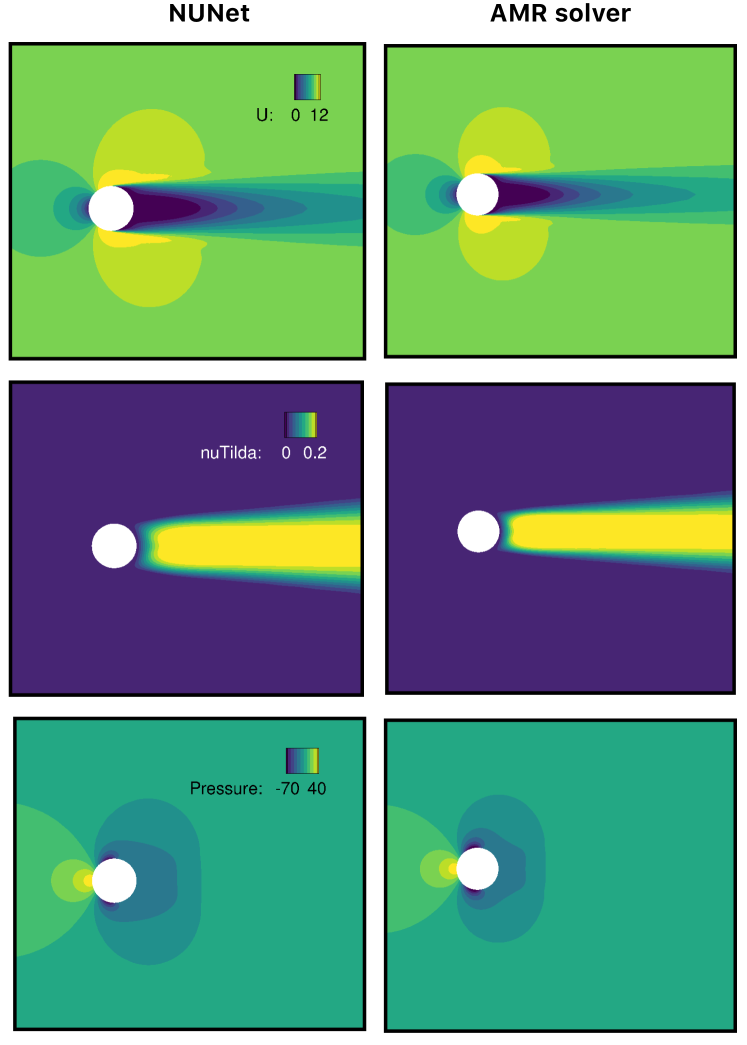
Figure 12: Flow around a cylinder at Re = $1105$. Velocity in $\mathrm{m}\text{\,}{\mathrm{s}}^{-1}$ (top), kinematic pressure in $\mathrm{m}^{2}\mathrm{/}\mathrm{s}^{2}$ (bottom), and modified eddy viscosity in $\mathrm{m}^{2}\mathrm{/}\mathrm{s}$ (middle). Comparison between NUNet’s result and the AMR solver result for $b=4$ levels of refinement.

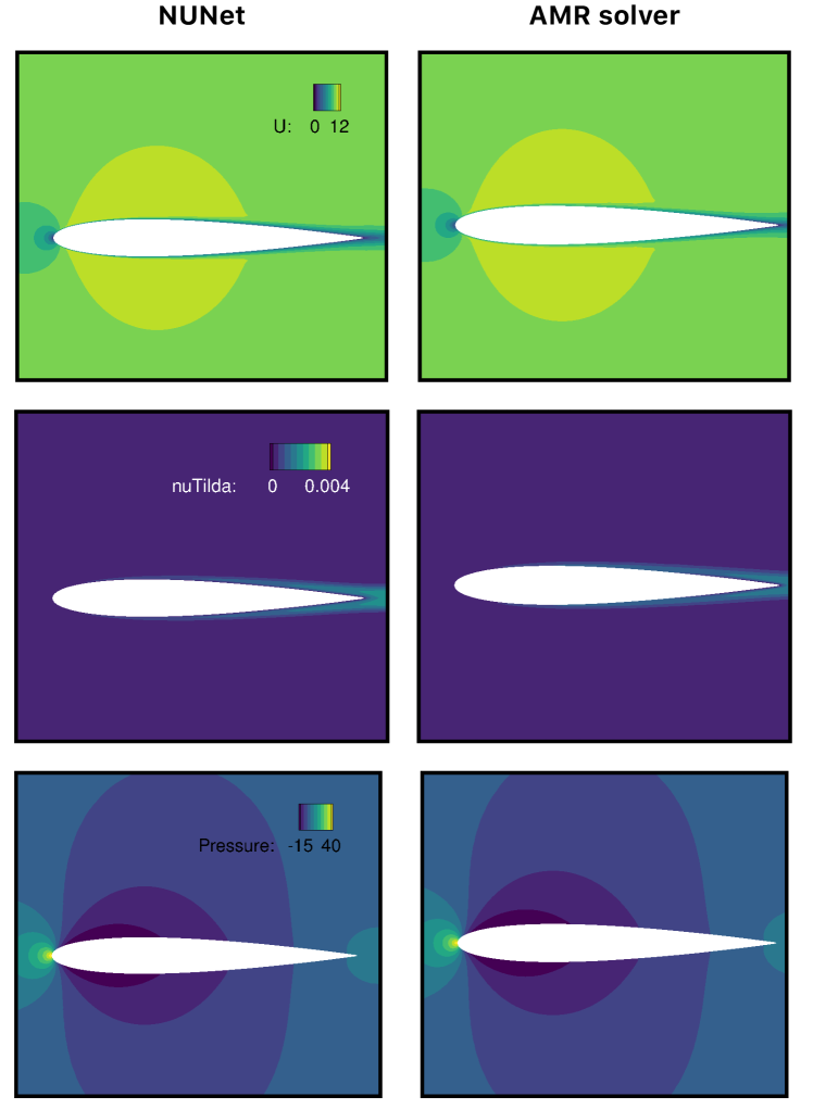
Figure 13: Flow around the symmetric NACA0012 airfoil at Re = $2.5104$. Velocity in $\mathrm{m}\text{\,}{\mathrm{s}}^{-1}$ (top), kinematic pressure in $\mathrm{m}^{2}\mathrm{/}\mathrm{s}^{2}$ (bottom), and modified eddy viscosity in $\mathrm{m}^{2}\mathrm{/}\mathrm{s}$ (middle). Comparison between NUNet’s result and the AMR solver result for $b=4$ levels of refinement.

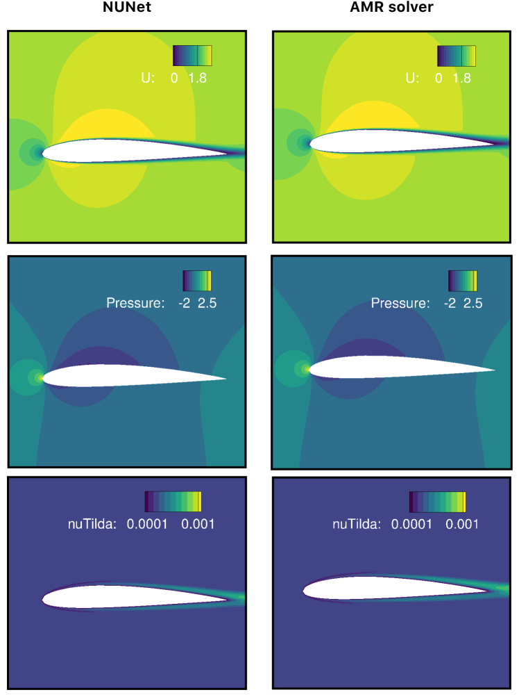
Figure 14: Flow around the non-symmetric NACA1412 airfoil at Re = $2.5104$. Velocity in $\mathrm{m}\text{\,}{\mathrm{s}}^{-1}$ (top), kinematic pressure in $\mathrm{m}^{2}\mathrm{/}\mathrm{s}^{2}$ (bottom), and modified eddy viscosity in $\mathrm{m}^{2}\mathrm{/}\mathrm{s}$ (middle). Comparison between NUNet’s result and the AMR solver result for $b=4$ levels of refinement.

5.1.2 Quantitative results

We present a quantitative comparison between NUNet and the AMR solver using a grid convergence study. We report, for the flat plate test cases, the coefficient of friction ($C_{f}$) at $x=0.95L$, where $L$ is the length of the flat plate. For the channel flow test cases, we also report the $C_{f}$ on the lower wall at $x=0.95L$. For the cylinder and airfoil test cases, we monitor the coefficient of drag or $C_{D}$. Figure 15 shows the value of the QoI for each test case with increasing refinement level $n$.

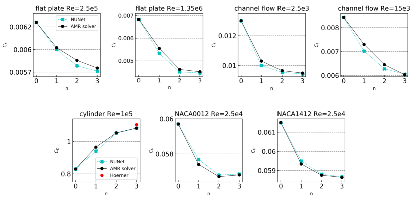
Figure 15: Value of the QoI versus refinement level $n$ for NUNet (blue) and the AMR solver (black) for each test case. $C_{f}$ refers to coefficient of friction, and $C_{D}$ to coefficient of drag. The red dot is the experimental value for the cylinder case found in [47]. Both algorithms converge as we increase the mesh refinement level from the original coarse mesh.

We make two main observations from the plots in Figure 15. First, we observe a good agreement between the QoI reported by NUNet and the AMR solver at all levels of refinement. At $n=0$, the value of the QoI is the same because they start with the same coarse mesh. Second, we observe how NUNet’s and the AMR solver’s reported QoI show a notable convergence trend after $n=1$. The plot referring to the cylinder case in Figure 15 shows, in red, the experimental value of $C_{D}$ reported in Hoerner [47], which is $1.108$, while NUNet reports $1.0835$, a $2.2\%$ deviation, and the AMR solver reports $1.085$, a $2.1\%$ deviation. These errors are in line with those in the literature when comparing experimental results with RANS simulations using the SA model [48].

5.2 Performance Analysis of NUNet

In this section , we evaluate NUNet’s performance. We first compare its time-to-convergence (TTC) with the AMR solver’s TTC in obtaining the results in Figure 15 at $n=3$. Recall that NUNet’s TTC is the sum of the inference time and the time the physics solver takes to drive the solution from inference to convergence. Table 1 shows these times and reports the iterations-to-convergence (ITC) taken by both the physics solver and the AMR solver. For the channel flow case, NUNet achieves a $4.3\times$ speedup for the interpolated boundary condition case. For the flat plate, we obtain a $5.5\times$ (interpolated case) and a $4.7\times$ speedup (extrapolated case) over the AMR solver. NUNet obtains an impressive $3.2\times$ speedup for a flow around a cylinder, which is an unseen-during-training geometry. The cylinder case is the most challenging test case for NUNet since accurately predicting the wake region behind the cylinder (as seen in Figure 12), a region with highly nonlinear, complex flow behavior, is challenging. Therefore, the physics solver spends a significant amount of time fixing that region and its speedup is the lowest among all test cases. Overall, NUNet refines regions of interest such as near-wall areas (channel flow and flat plate) and the wake behind the solid body (cylinder), shows excellent grid convergence properties, and significantly accelerates the traditional AMR solver by $3.2-5.5\times$.

	AMR solver		NUNet
	ITC	TTC	ITC	TTC inf + ps	speedup
channel flow Re = $2.5103$	3369	3	2261	$1.210-2$ + 0.68	4.3$\times$
channel flow Re = $15103$	4940	3.1	2022	$1.110-1$ + 0.8	3.8$\times$
flat plate Re = $2.5105$	3389	2.7	1364	$810-3$ + 0.48	5.5$\times$
flat plate Re = $1.35106$	5000	2	2214	$910-3$ + 0.42	4.7$\times$
cylinder Re = $1105$	11155	4.8	4598	$6.310-3$ + 1.5	3.2$\times$
N0012 Re = $2.5104$	2267	2	1150	$510-3$ + 0.55	3.5$\times$
N1412 Re = $2.5104$	2637	2.1	1720	$510-3$ + 0.62	3.3$\times$

Table 1: Comparison of the time-to-convergence in minutes (TTC) and iterations-to-convergence (ITC) of NUNet and the AMR solver. For NUNet, we report separately the time spent in inference (inf) and the time spent by the physics solver (ps) driving the solution from inference to convergence, together with the speedup over the AMR solver.

Next, we evaluate NUNet’s performance by comparing it with a baseline neural network. Recall that one of the goals of this paper is to perform non-uniform super-resolution to avoid high-resolution inference in areas that do not require it. We hypothesize that NUNet is advantageous over SOTA methods that perform uniform super-resolution [13, 14, 16, 15] because these methods require $64\times$ larger labels for $64\times$ super-resolutions. To prove our hypothesis, we build the SURFNet [16] framework and use it as our baseline. We compare NUNet with SURFNet using two metrics. For a $64\times$ super-resolution, we report, first, the time to achieve the same accuracy. The SURFNet’s framework also consists of a DNN inference followed by a physics solver that guarantees convergence requirements. Hence, we compare both end-to-end frameworks and report both the inference time and the physics solver time. Second, we compare the memory consumption at inference. Because both NUNet and SURFNet perform inference on a CPU, we report these metrics on the CPU described in 4.4. The results are presented in Table 2.

	Memory usage			Time inf + ps
	SURFNet	NUNet	rf	SURFNet	NUNet	speedup
cf Re = $2.5103$	3.9	0.88	4.4$\times$	0.25 + 14	$1.210-2$ + 0.68	20.6$\times$
cf Re = $15103$	3.9	0.82	4.8$\times$	0.25 + 14.5	$1.110-2$ + 0.8	18.2$\times$
fp Re = $2.5105$	3.9	0.62	6.3$\times$	0.25 + 11	$810-3$ + 0.48	23$\times$
fp Re = $1.35106$	3.9	0.68	5.7$\times$	0.25 + 12	$910-3$ + 0.42	28.5$\times$
cyl Re = $1105$	3.9	0.52	7.5$\times$	0.25 + 10.3	$6.310-3$ + 1.5	7$\times$
N0012 Re = $2.5104$	3.9	0.54	7.2$\times$	0.25 + 8.35	$510-3$ + 0.55	15.5$\times$
N1412 Re = $2.5104$	3.9	0.51	7.65$\times$	0.25 + 8.6	$510-3$ + 0.62	14.1$\times$

Table 2: Comparison of NUNet with SURFNet. Left column compares the GB of memory consumed at each test case’s inference and shows the reduction factor (rf) achieved by NUNet. Right column compares, in minutes, the inference time (inf) and the time to convergence by the physics solver (ps) of both approaches and shows NUNet’s speedup over SURFNet. cf = channel flow, fp = flat plate, cyl = cylinder, N0012 = NACA0012 (symmetric airfoil), and N1412 = NACA1412 (non-symmetric airfoil).

Table 2’s shows that NUNet significantly outperforms SURFNet for a $64\times$ super-resolution for all test cases. Specifically, we observe $7-28.5\times$ speedups over SURFNet. We observe the same behavior with the memory usage at inference. SURFNet requires almost 4 GB whereas NUNet significantly reduces the memory consumption, realizing $4.4-7.5\times$ reduction factors. Note that NUNet’s inference time and memory usage is not consistent through the test cases because the fine/coarse regions change, as opposed to SURFNet that performs uniform super-resolution.

6 Conclusions

This paper presented NUNet, a deep learning algorithm that predicts adaptive mesh refinement. It is an end-to-end framework for non-uniform super-resolution of turbulent flows that predicts high-resolution accuracy only in specific regions of the domain while keeping areas with less complex flow features in the low-precision range for scalability and performance. NUNet is trained with low-resolution data from three different canonical flows and predicts non-uniform flow fields for flow cases that have boundary conditions/geometries unseen during training. NUNet shows excellent discerning properties in all test cases, producing higher resolution outputs in regions with complex flow features, such as near-wall areas or the wake region behind a cylinder, and keeping low-resolution patches in those areas that have smooth variations, such as the flow freestream.

NUNet reaches the same convergence guarantees as traditional AMR solvers, shows excellent quantitative agreement with their heuristics, and accelerates them by $3.2-5.5\times$ in all test cases. Due to its ability to super-resolve only regions of interest, it reduces the end-to-end time and the memory usage by $7-28.5\times$ and $4.4-7.65\times$, respectively, over state-of-the-art DL methods that perform uniform super-resolution. Future work includes experimenting with different combinations of the number of bins, larger domains with larger patch sizes, different binning strategies, and generalization to a larger class of geometries and boundary conditions.

7 Acknowledgement

This work was partly supported by the National Science Foundation (NSF) under the award number 1750549. Any opinions, findings and conclusions expressed in this material are those of the authors and do not necessarily reflect those of NSF. We thank the HPC3 cluster at the University of California, Irvine, for providing the required hardware to conduct this research.

References

- Pope [2001] Stephen B Pope. Turbulent flows, 2001.
- Lee et al. [2013] Myoungkyu Lee, Nicholas Malaya, and Robert D Moser. Petascale direct numerical simulation of turbulent channel flow on up to 786k cores. pages 1–11, 2013.
- Jasak et al. [2007] Hrvoje Jasak, Aleksandar Jemcov, Zeljko Tukovic, et al. Openfoam: A c++ library for complex physics simulations. In International workshop on coupled methods in numerical dynamics, volume 1000, pages 1–20. IUC Dubrovnik Croatia, 2007.
- Reynolds [1895] Osborne Reynolds. Iv. on the dynamical theory of incompressible viscous fluids and the determination of the criterion. Philosophical transactions of the royal society of london.(a.), (186):123–164, 1895.
- Mostafazadeh Davani et al. [2017] Bahareh Mostafazadeh Davani, Ferran Marti, Behnam Pourghassemi, Feng Liu, and Aparna Chandramowlishwaran. Unsteady navier-stokes computations on GPU architectures. In 23rd AIAA Computational Fluid Dynamics Conference, page 4508, 2017.
- Mostafazadeh et al. [2018] Bahareh Mostafazadeh, Ferran Marti, Feng Liu, and Aparna Chandramowlishwaran. Roofline guided design and analysis of a multi-stencil CFD solver for multicore performance. In Proc. 32nd IEEE Int’l. Parallel and Distributed Processing Symp. (IPDPS), pages 753–762, Vancouver, British Columbia, Canada, May 2018.
- [7] NACA0012 grids. https://turbmodels.larc.nasa.gov/naca0012numerics_grids.html.
- Ghia et al. [1982] UKNG Ghia, Kirti N Ghia, and CT Shin. High-re solutions for incompressible flow using the navier-stokes equations and a multigrid method. Journal of computational physics, 48(3):387–411, 1982.
- Salvadore et al. [2013] Francesco Salvadore, Matteo Bernardini, and Michela Botti. GPU accelerated flow solver for direct numerical simulation of turbulent flows. Journal of Computational Physics, 235:129–142, 2013.
- Dubey et al. [2021] Anshu Dubey, Martin Berzins, Carsten Burstedde, Michael L. Norman, Didem Unat, and Mohammed Wahib. Structured adaptive mesh refinement adaptations to retain performance portability with increasing heterogeneity. Computing in Science Engineering, 23(5):62–66, 2021. doi: 10.1109/MCSE.2021.3099603.
- Dosovitskiy et al. [2021] Alexey Dosovitskiy, Lucas Beyer, Alexander Kolesnikov, Dirk Weissenborn, Xiaohua Zhai, Thomas Unterthiner, Mostafa Dehghani, Matthias Minderer, Georg Heigold, Sylvain Gelly, et al. An image is worth 16x16 words: Transformers for image recognition at scale. International Conference on Learning Representations (ICLR), 2021.
- Devlin et al. [2018] Jacob Devlin, Ming-Wei Chang, Kenton Lee, and Kristina Toutanova. BERT: Pre-training of deep bidirectional transformers for language understanding. arXiv preprint arXiv:1810.04805, 2018.
- Jiang et al. [2020] Chiyu Max Jiang, Soheil Esmaeilzadeh, Kamyar Azizzadenesheli, Karthik Kashinath, Mustafa Mustafa, Hamdi A Tchelepi, Philip Marcus, Anima Anandkumar, et al. MeshfreeFlowNet: A Physics-Constrained Deep Continuous Space-Time Super-Resolution Framework. The International Conference for High Performance Computing, Networking, Storage, and Analysis (SC), 2020.
- Gao et al. [2021] Han Gao, Luning Sun, and Jian-Xun Wang. Super-resolution and denoising of fluid flow using physics-informed convolutional neural networks without high-resolution labels. Physics of Fluids, 33(7):073603, 2021.
- Fukami, Kai and Fukagata, Koji and Taira, Kunihiko [2021] Fukami, Kai and Fukagata, Koji and Taira, Kunihiko. Machine-learning-based spatio-temporal super resolution reconstruction of turbulent flows. Journal of Fluid Mechanics, 909, 2021.
- Obiols-Sales et al. [2021] Octavi Obiols-Sales, Abhinav Vishnu, Nicholas Malaya, and Aparna Chandramowliswharan. SURFNet: Super-resolution of turbulent flows with transfer learning using small datasets. In 30th International Conference on Parallel Architectures and Compilation Techniques (PACT), pages 1–11, 2021.
- Fukami et al. [2019] Kai Fukami, Koji Fukagata, and Kunihiko Taira. Super-resolution reconstruction of turbulent flows with machine learning. Journal of Fluid Mechanics, 870:106–120, 2019.
- Bhattacharya et al. [2020] Kaushik Bhattacharya, Bamdad Hosseini, Nikola B Kovachki, and Andrew M Stuart. Model reduction and neural networks for parametric pdes. arXiv preprint arXiv:2005.03180, 2020.
- Liu et al. [2020] Bo Liu, Jiupeng Tang, Haibo Huang, and Xi-Yun Lu. Deep learning methods for super-resolution reconstruction of turbulent flows. Physics of Fluids, 32(2):025105, 2020.
- Bryan et al. [2014] Greg L Bryan, Michael L Norman, Brian W O’Shea, Tom Abel, John H Wise, Matthew J Turk, Daniel R Reynolds, David C Collins, Peng Wang, Samuel W Skillman, et al. Enzo: An adaptive mesh refinement code for astrophysics. The Astrophysical Journal Supplement Series, 211(2):19, 2014.
- Zhang et al. [2021] Weiqun Zhang, Andrew Myers, Kevin Gott, Ann Almgren, and John Bell. AMReX: Block-structured adaptive mesh refinement for multiphysics applications. The International Journal of High Performance Computing Applications, page 10943420211022811, 2021.
- Obiols-Sales et al. [2020] Octavi Obiols-Sales, Abhinav Vishnu, Nicholas Malaya, and Aparna Chandramowliswharan. CFDNet: A deep learning-based accelerator for fluid simulations. In Proceedings of the 34th ACM International Conference on Supercomputing, pages 1–12, 2020.
- Maulik et al. [2019] Romit Maulik, Himanshu Sharma, Saumil Patel, Bethany Lusch, and Elise Jennings. Accelerating rans turbulence modeling using potential flow and machine learning. arXiv preprint arXiv:1910.10878, 2019.
- Berger and Oliger [1984] Marsha J Berger and Joseph Oliger. Adaptive mesh refinement for hyperbolic partial differential equations. Journal of computational Physics, 53(3):484–512, 1984.
- [25] Richardson Extrapolation. https://personal.math.ubc.ca/~israel/m215/rich/rich.html.
- Nemec et al. [2008] Marian Nemec, Michael Aftosmis, and Mathias Wintzer. Adjoint-based adaptive mesh refinement for complex geometries. In 46th AIAA Aerospace Sciences Meeting and Exhibit, page 725, 2008.
- Bohn and Feischl [2021] Jan Bohn and Michael Feischl. Recurrent neural networks as optimal mesh refinement strategies. Computers & Mathematics with Applications, 97:61–76, 2021.
- Kasmai et al. [2011] N Kasmai, D Thompson, E Luke, M Jankun-Kelly, and R Machiraju. Feature-based adaptive mesh refinement for wingtip vortices. International journal for numerical methods in fluids, 66(10):1274–1294, 2011.
- Yang et al. [2021] Jiachen Yang, Tarik Dzanic, Brenden Petersen, Jun Kudo, Ketan Mittal, Vladimir Tomov, Jean-Sylvain Camier, Tuo Zhao, Hongyuan Zha, Tzanio Kolev, et al. Reinforcement learning for adaptive mesh refinement. arXiv preprint arXiv:2103.01342, 2021.
- Lu et al. [2021] Lu Lu, Xuhui Meng, Zhiping Mao, and George Em Karniadakis. Deepxde: A deep learning library for solving differential equations. SIAM Review, 63(1):208–228, 2021.
- Asahi et al. [2021] Yuuichi Asahi, Sora Hatayama, Takashi Shimokawabe, Naoyuki Onodera, Yuta Hasegawa, and Yasuhiro Idomura. Amr-net: Convolutional neural networks for multi-resolution steady flow prediction. In 2021 IEEE International Conference on Cluster Computing (CLUSTER), pages 686–691. IEEE, 2021.
- Dong et al. [2014] Chao Dong, Chen Change Loy, Kaiming He, and Xiaoou Tang. Learning a deep convolutional network for image super-resolution. In European conference on computer vision, pages 184–199. Springer, 2014.
- Ledig et al. [2017] Christian Ledig, Lucas Theis, Ferenc Huszár, Jose Caballero, Andrew Cunningham, Alejandro Acosta, Andrew Aitken, Alykhan Tejani, Johannes Totz, Zehan Wang, et al. Photo-realistic single image super-resolution using a generative adversarial network. In Proceedings of the IEEE conference on computer vision and pattern recognition, pages 4681–4690, 2017.
- Yang et al. [2020] Fuzhi Yang, Huan Yang, Jianlong Fu, Hongtao Lu, and Baining Guo. Learning texture transformer network for image super-resolution. In Proceedings of the IEEE/CVF Conference on Computer Vision and Pattern Recognition, pages 5791–5800, 2020.
- Cordonnier et al. [2021] Jean-Baptiste Cordonnier, Aravindh Mahendran, Alexey Dosovitskiy, Dirk Weissenborn, Jakob Uszkoreit, and Thomas Unterthiner. Differentiable patch selection for image recognition. In Proceedings of the IEEE/CVF Conference on Computer Vision and Pattern Recognition, pages 2351–2360, 2021.
- Lu et al. [2019] Lu Lu, Pengzhan Jin, and George Em Karniadakis. Deeponet: Learning nonlinear operators for identifying differential equations based on the universal approximation theorem of operators. arXiv preprint arXiv:1910.03193, 2019.
- Li et al. [2020] Zongyi Li, Nikola Kovachki, Kamyar Azizzadenesheli, Burigede Liu, Kaushik Bhattacharya, Andrew Stuart, and Anima Anandkumar. Fourier neural operator for parametric partial differential equations. arXiv preprint arXiv:2010.08895, 2020.
- Li, Zongyi and Kovachki, Nikola and Azizzadenesheli, Kamyar and Liu, Burigede and Bhattacharya, Kaushik and Stuart, Andrew and Anandkumar, Anima [2020] Li, Zongyi and Kovachki, Nikola and Azizzadenesheli, Kamyar and Liu, Burigede and Bhattacharya, Kaushik and Stuart, Andrew and Anandkumar, Anima. Neural operator: Graph kernel network for partial differential equations. arXiv preprint arXiv:2003.03485, 2020.
- Thuerey et al. [2019] Nils Thuerey, Konstantin Weißenow, Lukas Prantl, and Xiangyu Hu. Deep learning methods for reynolds-averaged navier–stokes simulations of airfoil flows. AIAA Journal, pages 1–12, 2019.
- Rall and Corliss [1996] Louis B Rall and George F Corliss. An introduction to automatic differentiation. Computational Differentiation: Techniques, Applications, and Tools, 89, 1996.
- Spalart and Allmaras [1992] Philippe Spalart and Steven Allmaras. A one-equation turbulence model for aerodynamic flows. In 30th aerospace sciences meeting and exhibit, page 439, 1992.
- Moin and Kim [1982] Parviz Moin and John Kim. Numerical investigation of turbulent channel flow. Journal of fluid mechanics, 118:341–377, 1982.
- Kingma and Ba [2014] Diederik P Kingma and Jimmy Ba. Adam: A method for stochastic optimization. arXiv preprint arXiv:1412.6980, 2014.
- Penttinen et al. [2011] Olle Penttinen, Ehsan Yasari, and Håkan Nilsson. A pimplefoam tutorial for channel flow, with respect to different les models. Practice Periodical on Structural Design and Construction, 23(2):1–23, 2011.
- Eça and Hoekstra [2014] Luis Eça and Martin Hoekstra. A procedure for the estimation of the numerical uncertainty of cfd calculations based on grid refinement studies. Journal of computational physics, 262:104–130, 2014.
- Ott [2002] Edward Ott. Chaos in dynamical systems. Cambridge university press, 2002.
- Hoerner [1965] Sighard F Hoerner. Fluid-dynamic drag. Hoerner fluid dynamics, 1965.
- Bao et al. [2011] Yan Bao, Dai Zhou, Cheng Huang, Qier Wu, and Xiang-qiao Chen. Numerical prediction of aerodynamic characteristics of prismatic cylinder by finite element method with spalart–allmaras turbulence model. Computers & structures, 89(3-4):325–338, 2011.