Discovering dynamical features of Hodgkin-Huxley-type model of physiological neuron using artificial neural network

Abstract

We consider Hodgkin-Huxley-type model that is a stiff ODE system with two fast and one slow variables. For the parameter ranges under consideration the original version of the model has unstable fixed point and the oscillating attractor that demonstrates bifurcation from bursting to spiking dynamics. Also a modified version is considered where the bistability occurs such that an area in the parameter space appears where the fixed point becomes stable and coexists with the bursting attractor. For these two systems we create artificial neural networks that are able to reproduce their dynamics. The created networks operate as recurrent maps and are trained on trajectory cuts sampled at random parameter values within a certain range. Although the networks are trained only on oscillatory trajectory cuts, it also discover the fixed point of the considered systems. The position and even the eigenvalues coincide very well with the fixed point of the initial ODEs. For the bistable model it means that the network being trained only on one brunch of the solutions recovers another brunch without seeing it during the training. These results, as we see it, are able to trigger the development of new approaches to complex dynamics reconstruction and discovering. From the practical point of view reproducing dynamics with the neural network can be considered as a sort of alternative method of numerical modeling intended for use with contemporary parallel hard- and software.

1 Introduction

Application of artificial neural networks in nonlinear dynamics in some aspects is a well developed area. Basically this is related to system modeling, state space reconstruction and time series forecasting. A comprehensive survey is beyond the scope of our paper, however some interesting topics, both early and contemporary, can be mentioned: adaptive system modeling and control using neural networks [1], reconstruction of the El Niño attractor with neural networks [2], using neural networks for combined state space reconstruction and forecasting [3], reconstruction of chaotic time series by neural networks [4], reconstructing a dynamical system and forecasting with deep neural networks [5]. However in view of the current success of deep learning in various areas, the use of machine learning methods for complex dynamics analysis can be extended. The promising perspective is related with generalization ability of the networks. If a network is trained on data generated by a dynamical system there are reasons to expect that it will extract the essence of the trained data. The subsequent evaluation of the network will result in discovering new features otherwise unnoticed. Another promising perspective is related with the fact that the neural networks can be treated as universal approximators [6, 7, 8, 9, 10]. A neural network can be trained to recover almost any, even very complicated, functional dependence. In particular it means that the networks can be used to model dynamical systems. Along with the generalization properties it potentially can open interesting perspectives in new approaches state space reconstruction and forecasting as well as revealing new dynamical properties. From the practical point of view reproducing dynamics with the neural network can be considered as a sort of alternative method of numerical modeling intended for use with contemporary parallel hard- and software. In particular it is suitable for so called AI accelerators, a hardware dedicated to deal with artificial neural networks [11, 12, 13].

In this paper we focus on dynamics modeling using neural networks. Previously we considered a simple two layer network as a recurrent map that is able to model various dynamical systems including Lorenz system, Rössler system and also the Hindmarsh–Rose model [14]. For these three examples the created neural network map demonstrated high quality of reconstruction including recovery of the Lyapunov spectra. However the dynamics of the well known Hodgkin-Huxley-type model [15] with two fast and one slow variables is found to require a more sophisticated approach. In this paper we create and analyze an artificial neural network that is able to reproduce this dynamics. For the considered parameter ranges the system has unstable fixed point and oscillating attractor that can be either bursting or spiking. Also a modification to the Hodgkin-Huxley-type model is considered that introduces bistability: an area in the parameter space appears where the fixed point becomes stable and coexists with the bursting attractor. The created network operates as a recurrent map, i.e., it reproduces the dynamics as a discrete time system. This is trained as a feedforward network using standard back propagation routine on trajectory cuts sampled at random parameter values within a certain range. The network structure is developed to take into account the different time scales of the variables of the modeled system. Although the network is trained only on oscillatory trajectory cuts, the resulting recurrent map also discovers the fixed point whose position and even the eigenvalues coincide well with the fixed point of the initial ODE system. In particular it means that when a bistable regime is modeled, the network being trained on one brunch of solutions discovers another one, never seen in the course of training.

Before embarking on our study we need to mention another interesting approach to modeling dynamics using the machine learning methods. In papers [16, 17] chaotic dynamics is recovered using so called reservoir computing system. This system operates as a recurrent map and its training is similar to the training of the recurrent neural network. The training dataset comprises a set of long trajectories computed at various parameter values and the training is done on them at once. The reservoir computing system includes high dimensional iterations of the hidden layer vector. The iterations include a multiplication by a non-trainable random matrix and application of a nonlinear function. The modeled dynamical variable after multiplication by also non-trainable random input matrix is added to the hidden layer vector before each iteration, the iteration is done and then a value of the dynamical variable at the next time step is computed as a result of multiplication of the obtained hidden layer vector by an output matrix. It is the only matrix whose elements are tuned in course of the training. The approach based on reservoir computing demonstrates the successful prediction of critical transition [16], reveals of the emergence of transient chaos [17], allows performing time series analysis [18].

The difference of our approach is that the state space dimension of our neural network model is exactly the same as for the modeled dynamics. It does not include any random non-trainable matrices. The resulting recurrent map is written in an explicit form and admits its analysis: we are able to find analytical expressions for the Jacobian matrix and analyze its eigen values.

The paper is organized as follows. First, in Sec. 2 we discuss the modeled system, then in Sec. 3 we introduce the neural network model and finally in Sec. 4 the dynamics of the neural network model is analyzed. In Sec. 5 the obtained results are outlined.

2 Modeled system

We consider the simplified pancreatic beta-cell model based on the Hodgkin-Huxley formalism [15]. In addition to the original system its modified version is also considered that includes bistability as suggested by Stankevich and Mosekilde [19]. This modification is introduced to demonstrate that an additional voltage-dependent potassium current that is activated in the region around the original, unstable equilibrium point results in the coexistence of a stable equilibrium point with a state of continuous bursting.

$$\tau\dot{V} =-I_{Ca}(V)-I_{K}(V,n)-I_{K2}(V)-I_{S}(V,S),$$ (1)

$$\tau\dot{n} =\sigma\,[n_{\infty}(V)-n],$$

$$\tau_{S}\dot{S} =S_{\infty}(V)-S.$$

Here, $V$ represents the membrane potential, $n$ may be interpreted as the opening probability of the potassium channels, and $S$ accounts for the presence of a slow variable in the system. The variables $I_{Ca}(V)$ and $I_{K}(V,n)$ are the calcium and potassium currents, $g_{Ca}$ and $g_{K}$ are the associated conductances, and $V_{Ca}$ and $V_{K}$ are the respective Nernst (or reversal) potentials. Together with $I_{S}(V,S)$, the slow calcium current $I_{Ca}$ and the potassium current $I_{K}$ define the three transmembrane currents, Eqs. (2), (3), and (4). The gating variables for $m$, $n$, and $S$ represent the opening probabilities of the fast and slow potassium channels, Eq. (6). The modification resulting in the stabilization of the equilibrium point is introduced as the voltage-dependent potassium current that varies strongly with the membrane potential right near this equilibrium point so that its stabilization can occur without affecting the global flow in the model. The suggested form of the potassium current is specified by Eq. (5) where the function (7) represents the opening probability for the introduced new type of potassium channel.

$$I_{Ca}(V)=g_{Ca}\,m_{\infty}(V)\,(V-V_{Ca}),$$ (2)

$$I_{K}(V,n)=g_{K}\,n\,(V-V_{K}),$$ (3)

$$I_{S}(V,S)=g_{S}\,S\,(V-V_{K}),$$ (4)

$$I_{K2}(V)=g_{K2}\,p_{\infty}(V)\,(V-V_{K}),$$ (5)

$$\omega_{\infty}(V)=\left(1+\exp\frac{V_{\infty}-V}{\theta_{\omega}}\right)^{-1},\hskip 11.99998pt\omega=m,n,S,$$ (6)

$$p_{\infty}(V)=\left(\exp\frac{V-V_{p}}{\theta_{p}}+\exp\frac{V_{p}-V}{\theta_{p}}\right)^{-1}.$$ (7)

Table 1: Numerical values of parameters of the model (1)

$\tau=0.02\,\text{s}$	$\tau_{S}=35\,\text{s}$	$\sigma=0.93$
$g_{Ca}=3.6$	$g_{K}=10$	$g_{S}=4$	$g_{K2}=0.12$
$V_{Ca}=25\,\text{mV}$	$V_{K}=-75\,\text{mV}$
$\theta_{m}=12\,\text{mV}$	$\theta_{n}=5.6\,\text{mV}$	$\theta_{S}=10\,\text{mV}$	$\theta_{p}=1\,\text{mV}$
$V_{m}=-20\,\text{mV}$	$V_{n}=-16\,\text{mV}$	$V_{S}=-36\,\text{mV}$	$V_{p}=-49.5\,\text{mV}$

We will consider the system (1) for $V_{S}$ varying within the range $[-40,-30]$ while all other numerical values of parameters are listed in Tab. 1. Parameter $g_{K2}$ is responsible for switching the modification that introduces the bistability as discussed above. Setting $g_{K2}=0$ we obtain the original system. This system has an unstable fixed point. For example for $V_{S}=-36$ the fixed point is $V=-49.897$, $n=2.3452\times 10^{-3}$, and $S=0.19946$. Its instability is indicated by the positive largest eigenvalue: $\mu_{1}=20.772$, $\mu_{2}=9.0834\times 10^{-2}$, $\mu_{3}=-42.884$. Dynamics of the system (1) in this case is illustrated in Fig. 1. Panels (a,b,c) represent busting oscillations at $V_{s}=-36$. One can see that the variables $V$ and $n$ vary fast while $S$ is slow. Figure 2(a) shows the corresponding three-dimensional phase portrait of the bursting attractor. When $V_{S}$ gets larger the bifurcation occurs and after that the system demonstrates periodic spiking, see Fig. 1 (d,e,f) plotted at $V_{S}=-33$.

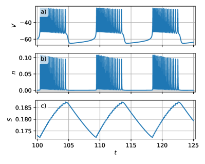
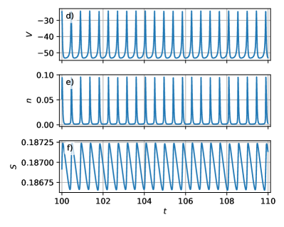
Figure 1: Time series of the original system (1), i.e., at $g_{K2}=0$. Panels (a,b,c): bursting oscillations at $V_{S}=-36$. Panels (d,e,f) spiking regime at $V_{S}=-33$. Other parameters see in Tab. 1.

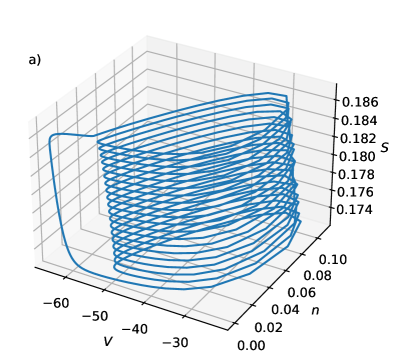
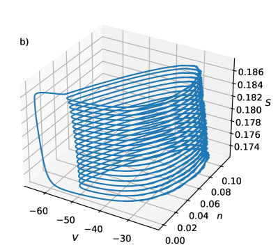
Figure 2: (a) Three-dimensional plot of the bursting attractor of the original system (1). Parameters are as in Fig. 1(a,b,c). (b) Attractor of the corresponding neural network map (8) trained to recover the original system in panel (a).

Figure 3(a) shows how dynamics of the original system (1) at $g_{K2}=0$ changes as $V_{S}$ is varied. We will call it bifurcation diagram. Here $V_{S}$ varies along the horizontal axis, time goes vertically and shades of color indicate values of dynamical variable $V$ recorded after omitting transients (100 time units): darker color corresponds to higher $V$. The data for this figure are computed while moving along $V_{S}$ from left to right. Without a special taking care the bursting clusters at successive parameter steps emerge shifted in time so that the neighboring patterns in the plot are not adjusted and the whole picture is obscured. To improve the clarity we compute each new solution (after dropping out the transients) over the doubled time interval, i.e. for 30 time units instead of the used in the figure 15. Then within this longer solution we seek for a window that has the smallest Euclidean distance with the solution already selected for the previous step. As a result in Fig. 3(a) the area of bursting oscillations is shown as two stripes that disappears at the bifurcation point $V_{S}\approx-33.73$. To the right of this point high frequency spiking oscillations appear that are represented in the diagram as a more or less uniform texture.

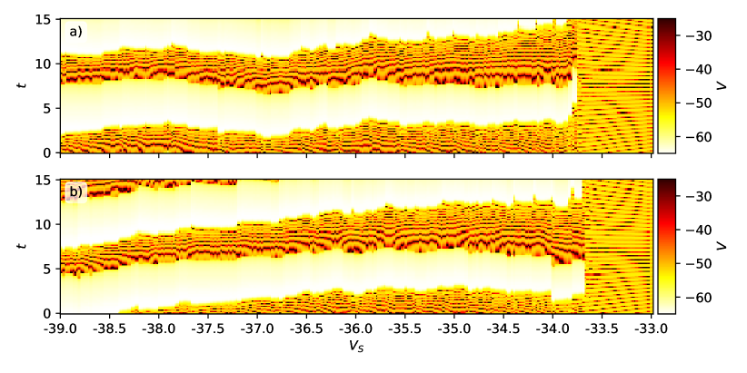
Figure 3: (a) Bifurcation diagram of the original system (1) at $g_{K2}=0$, i.e., without the bistability. Time dependence of $V$ is shown along the vertical axis with color shades, the darker the higher. Its modification with $V_{S}$ is demonstrated along the horizontal axis. (b) Bifurcation diagram computed with the corresponding neural network map (8) trained to recover the original system.

As discussed above the modification is engaged at nonzero $g_{K2}$: within a certain range of $V_{S}$ the fixed point becomes stable, and it coexists with the stable bursting attractor. At $g_{K2}=0.12$ and $V_{S}=-36$ the fixed point is $V=-50.636$, $n=2.0560\times 10^{-3}$, $S=0.18792$, and its stability is indicated by the negative largest eigenvalue: $\mu_{1}=-0.15927$, $\mu_{2}=-19.521$, $\mu_{3}=-38.785$. Dynamics of the modified system is illustrated in Fig. 4. Bursting oscillations at $V_{S}=-36$ are shown in Fig. 4(a,b,c) and spiking oscillations at $V_{S}=-33$ are in Fig. 4(d,e,f). Observe that that the bursting and spiking of the modified bistable system are visually almost indistinguishable with those for the original system, cf. Fig.1. The three-dimensional view of the bursting attractor in this case also looks the same as for the original system in Fig. 2(a) and is not shown.

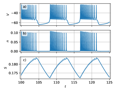
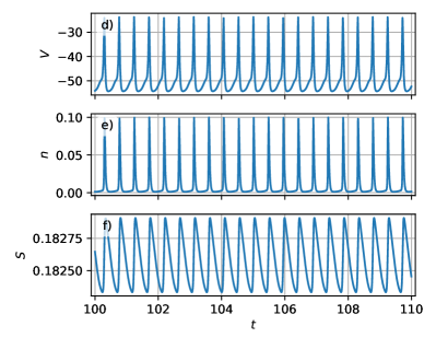
Figure 4: Time series of the modified system (1) at $g_{K2}=0.12$. (a,b,c) Bursting at $V_{S}=-36$. (d,e,f) Spiking at $V_{S}=-33$.

Coexistence of bursting and silent states in the modified system (1) at $g_{K2}$ is illustrated in the bifurcation diagrams in Fig. 5. Axes and color encoding are the same as in Fig. 3. To compute data for Fig. 5(a) we take the starting point at $V_{S}=-36$ sufficiently far from the fixed point, compute a solution and then find solutions moving to the left along the parameter axis with the inheritance: starting point for the next parameter value is taken as the solution from the previous point. Solutions are adjusted in time to provide more clear picture in the same way as for Fig. 3. Then we move in the same way from $V_{S}=-36$ to the right. Figure 5(b) is computed in the same way, but the initial staring point is taken close to the fixed point. We see the presence of the bistability area in the middle parts of the plots: in Fig. 5 solutions initiated far from the fixed point demonstrate bursting while trajectories started in the vicinity of the fixed point converge to it. Figure 5(c), blue curve, shows how the largest real part of the eigenvalues $\mathop{\mathrm{Re}}\mu_{1}$ of the fixed point depends on the parameter. We see that in accordance with the observations in Fig. 5(a,b) the fixed point has the negative eigenvalues in the middle area so that it is stable and coexists with the bursting attractor.

The stable fixed point has a very small basin of attraction and, consequently, there is very low probability that the system will arrive at it from random initial conditions. To demonstrate it we consider a cube $V\in[-70,-10]$, $n\in[0,0.12]$, and $S\in[0.17,0.2]$ that is large enough to cover both the bursting attractor and the fixed point for any $V_{S}$ within the considered range. For each $V_{S}$ we start 500 trajectories from random points within this cube and count how many of them arrive at the fixed point. The corresponding relative frequency $P_{\text{fxp}}$ is shown in Fig. 5(c) with the red curve. We observe that $P_{\text{fxp}}$ oscillates near one - three percents.

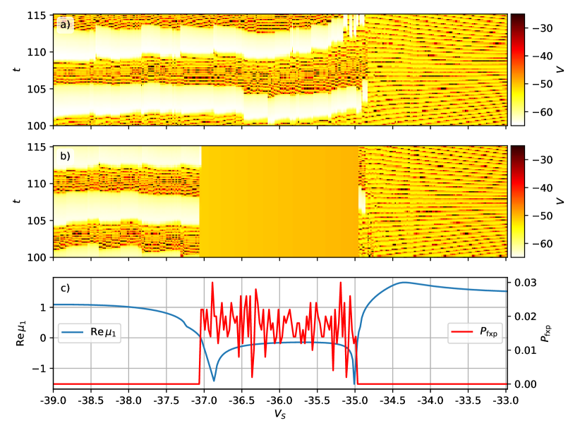
Figure 5: Bifurcation diagrams of the modified system (1) at $g_{K2}=0.12$. Panels (a) and (b) are computed with inheritance for two branches of solutions. Smooth area in the middle of the panel (b) indicate the stable fixed point. Panel (c) shows the largest real part of the eigenvalues of the fixed point (blue color). To improve the visibility positive values are plotted as $\log_{10}(\mathop{\mathrm{Re}}\mu_{1}+1)$ while the negative values are plotted as they are. Red curve in the panel (c) shows the relative frequency $P_{\mathrm{fxp}}$ of the stable fixed point implementation for random initial conditions, scale for it in right.

3 Neural network map

Now we turn to reproducing the dynamics of the original and modified versions of the system (1) using an artificial neural network. Our goal is to create the network that can be described as an explicit recurrent map of the form $u(t+\Delta t)=F(u(t),p,w)$, where $\Delta t$ is a constant time step, $u$ is a vector of dynamical variables, $p$ is a vector of control parameters, and $w$ is a collection of inner parameters that are tuned in course of the network training to obtain the desirable behavior.

Although we build a network that will operate as a recurrent map, it is created and trained as a feed forward network. We avoid using a recurrent network architecture since simple recurrent cells have the well known problems like exploding gradients, i.e., instabilities in course of training, and fast decaying memory [20]. These problems have been solved for more effective recurrent cells like LSTM or GRU, but they have complicated inner structure that discourages their subsequent consideration as dynamical systems prone to theoretical analysis. Also we do not consider an approach based on reservoir computing since the state space dimension of a system on the basis of the reservoir is much higher then the dimension of the modeled system [16, 17].

In our previous work [14] we considered a neural network model for nonlinear dynamical systems in a form of the recurrent map $u_{n+1}=u_{n}+\sigma(u_{n}A_{0}+pB_{0}+a_{0})A_{1}+a_{1}$, where $p$ is a vector of control parameters, $A_{0,1}$ and $B_{0}$ are matrices, $a_{0,1}$ are vectors and $\sigma(x)=(1+e^{-x})^{-1}$ is a sigmoidal function. High quality of reproduction has been achieved for Lorenz and Rössler systems as well as for Hindmarsh-Rose model of neuronal activity. However the system (1) is found to require a more sophisticated approach. We address it to the presence of components with very different time scales: $V$ and $n$ vary very fast and $S$ is slow, see Figs. 1(a,b,c) and 4(a,b,c). It is known that ODEs with such property requires special stiff solvers. So the modeling of this dynamics with neural networks also requires an appropriate network architecture.

Analysis of the problem reveals that the key point for modeling stiff dynamics is to reproduce each dynamical variable separately. The following subnetwork structure is suggested for the $i$th variable:

$$u_{i}(t+\Delta t)=u_{i}(t)+f(u_{i}(t)a_{i}+\alpha_{i}+g(u(t)A_{i}+pB_{i}+\beta_{i}))b_{i}+\gamma_{i}.$$ (8)

Here $u_{i}(t)$ is a scalar variable, either $V(t)$, $n(t)$ or $S(t)$, and $u(t)$ is a full vector of these dynamical variables. As usual for neural network context we consider it is as a row vector. Its dimension is $D_{u}=3$. $p$ is a row vector of control parameters of dimension $D_{p}$. We consider only one varying parameter $V_{S}$ so that $D_{p}=1$. $a_{i}$, $\alpha_{i}$ and $\beta_{i}$ are row vectors of dimension $N_{h}$, while $b_{i}$ is a column vector of dimension $N_{h}$. $\gamma_{i}$ is a scalar. $A_{i}$ is $D_{u}$ by $N_{h}$ matrix. Its $i$th row is assumed to contain zeros only. $B_{i}$ is $D_{p}$ by $N_{h}$ matrix. Functions $f(\cdot)$ and $g(\cdot)$ are scalar and are assumed to be applied in element-wise manner to vector elements. Both the functions $f(\cdot)$ and $g(\cdot)$ and $N_{h}$ can in principle be chosen different for each subsystem but for the sake of simplicity we do not apply a thorough hyperparameter optimization to our network and take $N_{h}=100$ and hyperbolic tangent $f(x)=g(x)=\tanh(x)$ that work well. Table 2 contains the whole network hyperparameters list.

Table 2: Hyperparameters of the network and the datasets

$f(x)=g(x)=\tanh(x)$, $N_{h}=100$,

$S=1000$, $C=1000$, $N_{\text{ds}}=S\times C=10^{6}$,

$p_{\text{split}}=0.2$, $N_{\text{batch}}=1000$,

$t_{0}=200$, $\Delta t=0.005$.

The idea behind forming the structure of the map (8) is as follows. In view of the theorems treating neural networks as universal approximators [6, 7, 8, 9, 10] the form of the network for a scalar variable can be $u_{i}(t+\Delta t)=u_{i}(t)+f(u_{i}(t)a_{i}+\alpha_{i})b_{i}+\gamma_{i}$. This is two layer network with one hidden layer of dimension $N_{h}$ whose state is given by the output of $f(\cdot)$. Provided that $f(\cdot)$ is sigmoidal, e.g., the hyperbolic tangent, and $N_{h}$ is sufficiently large these two layers are enough to approximate almost any function with a required precision. In particular it is able to approximate the map that reproduces dynamics of $u_{i}$. Yet this structure does not take into account the vector of control parameters $p$ and other dynamical variables. We suggest to inject them as the output of another layer $h_{i}=g(u(t)A_{i}+pB_{i}+\beta_{i})$. As already mentioned above the matrix $A_{i}$ has zeros on its $i$th row so that the influence of the $i$th variable onto $h_{i}$ is eliminated. This is done to reduce complexity of the resulting recurrent map. Thus the full formula reads $u_{i}(t+\Delta t)=u_{i}(t)+f(u_{i}(t)a_{i}+\alpha_{i}+h_{i})b_{i}+\gamma_{i}$ that exactly correspond to Eq. (8).

Thus the map (8) is created as neural network whose weight coefficients are collected in the following matrices and vectors

$$w=\{a_{i},\alpha_{i},A_{i},B_{i},\beta_{i},b_{i},\gamma_{i}\;|\;i=1,2,3\}.$$ (9)

They have to be tuned in course of training.

Actual implementation of the network includes the following steps. First of all we need to take into account that contemporary neural network frameworks as well as their theoretical background assume that the datasets on which they operate are standardized, i.e. they have zero mean and unit standard deviation. Training on non standardized data will be highly ineffective. Thus the datasets engaged in training of our networks are standardized before training as follows:

$$u\to(u-m_{u})/s_{u},\;p\to(p-m_{p})/s_{p},$$ (10)

were $m_{u}$ and $m_{p}$ are vectors of mean vales of $u$ and $p$, respectively, and $s_{u}$ and $s_{p}$ are the corresponding standard deviations. The element-wise operations are assumed. All training routines are done for the rescaled data. When the network is in use we first rescale the initial states and the parameters according to Eqs. (10) then perform computations and finally apply the inverse of these transforms before showing the results.

The neural network uses the following operators. Operator $\mathop{\mathrm{Take}}(u,i)$ returns $i$th elements of a vector $u$, and $\mathop{\mathrm{Sans}}(u,i)$ returns the vector without its $i$th element. Operator $\mathop{\mathrm{Dense}}(x,W,b)=xW+b$ represents a standard dense layer that mathematically corresponds to an affine transformation of the vector with matrix $W$ and vector $b$. Notice that in our notation an activation function is not built-in into the dense layer. It will be applied separately. There is the matrix $A_{i}$ in (8) whose $i$th row contains zeros. For the actual network training and operation we use a matrix $A^{\prime}_{i}$ whose $i$th row is absent that fulfills the vector $u_{\neg\,i}$ whose $i$th is also removed. The square brackets $[\cdot,\cdot]$ are used to indicate concatenation of two vectors or matrices.

The neural network implementing the map (8) can be described as follows. It has two input vectors, $p=(V_{S})$ (actually the vector $p$ is one-dimensional) and $u=(V,n,S)$, Eq. (11). First $u$ is split into a scalar $u_{i}$ and a vector $u_{\neg\,i}$ (its $i$th element is absent), see Eq. (12). The layer (13) takes $u_{\neg\,i}$ and $p$ and computes $N_{h}$ dimensional vector $h_{i}$. This vector assembles the influence of the control parameters and of all but $i$th dynamical variables. This vector is added to the output of the next dense layer that process the $i$th component itself, Eq. (14). The result of this transformation is $N_{h}$ dimensional vector $q_{i}$ that finally goes to the third layer (15) whose output is the increment to the initial value $u_{i}$ to obtain a value at the next time step $v^{\prime}_{i}$ that is the network output. Doing in the same way for all $i=1,2,3$ we form a full output vector $v^{\prime}$.

$$p=\mathop{\mathrm{Input}}(),\;u=\mathop{\mathrm{Input}}(),$$ (11)

$$u_{i}=\mathop{\mathrm{Take}}(u,i),\;u_{\neg\,i}=\mathop{\mathrm{Sans}}(u,i),$$ (12)

$$h_{i}=g(\mathop{\mathrm{Dense}}([u_{\neg\,i},p],[A^{\prime}_{i},B_{i}],\beta_{i})),$$ (13)

$$q_{i}=f(\mathop{\mathrm{Dense}}(u_{i},a_{i},\alpha_{i})+h_{i}),$$ (14)

$$v^{\prime}_{i}=u_{i}+\mathop{\mathrm{Dense}}(q_{i},b_{i},\gamma_{i})$$ (15)

The network is trained as a feed forward network. The dataset is prepared as follows: choose the time step $\Delta t$, see Tab. 2, and prepare the dataset as a collection of $N_{\text{ds}}$ records ($p$, $u$, $v$), where $u$ is an initial point for Eqs (1) solved at the control parameters $p$ during time interval $\Delta t$ to obtain $v$. This dataset is split into training and validation parts with $N_{\text{ds}}(1-p_{\text{split}})$ records in the training part and $N_{\text{ds}}\,p_{\text{split}}$ for the validation, see Tab. 2 for $p_{\text{split}}$ value. The dataset preparation will be discussed in more detail below.

In course of training a pair of vectors $p$ and $u$ are fed at the input, the network response vector $v^{\prime}$ is computed, and it is compared with the correct value $v$ from the dataset. The loss function for the training is mean squared error:

$$L=\|v-v^{\prime}\|^{2}.$$ (16)

The goal of the training is to minimize $L$ on the dataset due to tuning its parameters $w$, Eq. (9). In the very beginning the parameters are initialized at random. The whole training dataset is shuffled and split into batches each of $N_{\text{batch}}$ records, see Tab. 2. Each batch is sent to the network and the loss function (16) is computed for the batch as well as its gradient $\nabla_{w}L$ with respect to $w$. Then it is used in a gradient descent step to compute updates to $w$. The simplest version of the gradient descent step reads

$$w\rightarrow w-\gamma\nabla_{w}L$$ (17)

where the step size scale $\gamma$ is a small parameter controlling the convergence. In actual computations instead of the simplest one a more sophisticated method is used called Adam [21]. The difference is that the step size scale $\gamma$ is not a constant, but is tuned according to the accumulated gradients on the previous steps. When all batches are processed this is called an epoch. The training dataset is shuffled again and a new epoch of training starts. Quality of the training is estimated after each epoch by feeding the network with the validation data and computing the loss function without updating $w$. We perform $2000$ epochs of training and after that the mean squared error on the validation data decay down to the level $10^{-7}$.

Two networks are created as described above, for the original as well as for the modified system (1). Having the same structures described by Eq. (8) the networks differ by sets of parameters $w$ obtained after training on two sets of data computed using Eqs. (8).

To create the datasets we fix ODEs (1) parameters either for the original, $g_{K2}=0$, or for the modified system, $g_{K2}=0.12$, see Tab. 1 and sample $C$ parameter vectors $p=(V_{S})$ from the uniform distribution on the range $[-40,-30]$. For each parameter value a random initial point is generated $u(0)=(V(0),n(0),S(0))$ sufficiently far from the fixed point to make sure that the trajectory even in the bistability case will not go to it. Then Eqs. (1) are solved starting from this point. After a transient $t_{0}$, see Tab. 2, the system arrives at bursting or spiking attractor and its points are recorded with time step $\Delta t$ in a row: $u(t_{0})$, $u(t_{0}+\Delta t)$, $u(t_{0}+2\Delta t)$, $u(t_{0}+3\Delta t)$, …Totally $S+1$ points are recorded. After that $S$ data records are composed as ($p$, $u(t_{0})$, $u(t_{0}+\Delta t)$), ($p$, $u(t_{0}+\Delta t)$, $u(t_{0}+2\Delta t)$), ($p$, $u(t_{0}+2\Delta t)$, $u(t_{0}+3\Delta t)$) and so on. Notice that when training the trajectory chunks are shuffled so that each batch is a random sample of pairs of points, not the whole cuts of trajectories.

Altogether the dataset is formed by $C$ chunks of trajectories. Each chunk corresponds to a certain parameter value $V_{S}$ and includes $S$ trajectory points sampled with the time step $\Delta t$ in a row on either bursting or spiking attractors. Fixed point is never recorded to the dataset even in the case of bistability when the fixed point is stable. Thus in course of training the network never sees it.

The structure of the dataset generated for training the networks are illustrated in Fig. 6. Figure 6(a) represents a typical example of time dependence of distance from the oscillating attractor and the fixed point. We observe the fixed point is clearly separated from the oscillating attractor so that the distance cannot be smaller then $10^{-2}$. Figures 6(b,c) show distances from the fixed point to the dataset points for the original and the modified systems, respectively. We see that the fixed point remains separated from the dataset for the whole parameter range.

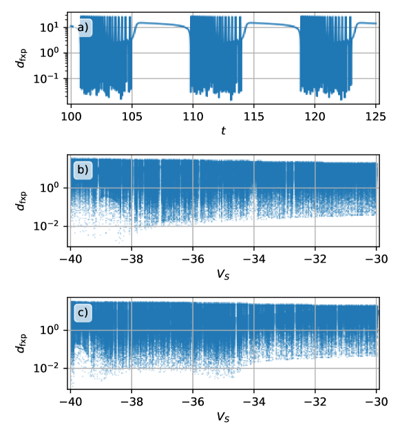
Figure 6: (a) Distance to the fixed point for a typical trajectory on the bursting attractor. (b) and (c) Distance to the fixed point for the dataset points used for training the neural network map (8) for the original and the modified systems, respectively.

Since the neural network map (8) has an explicit form we can explicitly compute its Jacobian matrix. This matrix is required both for a numerical routines finding the fixed point and for testing stability of the fixed point. The Jacobian matrix is found by differentiating right hand side of Eq. (8) by $u_{j}$, where $j=1,2,3$. After straightforward computations we can write the following expressions for the diagonal and off-diagonal elements of the matrix:

$$\begin{gathered}j_{ii}=1+a_{i}\mathop{\mathrm{Diag}}f^{\prime}(z_{i})b_{i},\\ j_{ij}=\mathop{\mathrm{Row}}(A_{i},j)\mathop{\mathrm{Diag}}g^{\prime}(y_{i})\mathop{\mathrm{Diag}}f^{\prime}(z_{i})b_{i},\\ z_{i}=u_{i}a_{i}+\alpha_{i}+g(y_{i}),\\ y_{i}=uA_{i}+pB_{i}+\beta_{i}\end{gathered}$$ (18)

Here operator $\mathop{\mathrm{Diag}}(x)$ creates a diagonal matrix whose diagonal consists of elements of vector $x$. Operator $\mathop{\mathrm{Row}}(X,i)$ returns a row vector whose elements are taken as $i$th row of the matrix $X$.

4 Dynamics of the neural network map

Using the described above architecture and datasets we have trained two neural network maps of the form (8) that reproduce dynamics of the original and modified versions of the system (1). Let us first demonstrate how these networks learn the attractors that were shown them during the training. Figure 7 demonstrates solutions computed as iteration of the neural network map (8) for the original system at the same parameters as ODEs in Fig. 1. Figure 8 represents solution computed using the map (8) for the modified system. The parameter values are as in Fig. 4. Observe very high similarity of trajectories of the neural network maps with the corresponding ODEs solutions. Figure 2(a,b) compares three dimensional views of the bursting attractors for the original system (1) and the corresponding neural network map (8), respectively. Observe again that the plots are very similar.

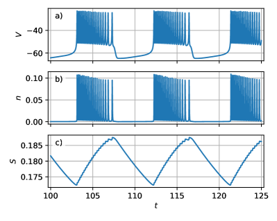
Figure 7: Time series same as in Fig.1 for the neural network map (8) trained to reproduce the original system.

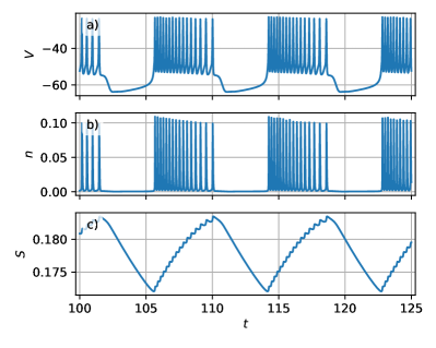
Figure 8: Time series same as Fig.4 for the neural network map (8), modified system.

Bifurcation diagrams for the original system (1) and for the corresponding neural network map (8) are shown in Fig. 3(a,b), respectively. We see the very high similarity again. The bifurcation diagrams for the modified system with bistability computed with ODEs (1) and with the neural network map (8) are compared in Figs. 5(a,b) and 9(a,b), respectively. We observe again a remarkable correspondence.

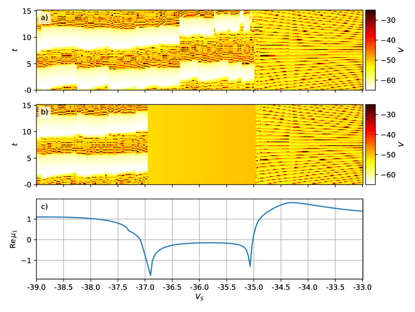
Figure 9: Bifurcation diagram for the neural network map (8) trained for the modified system with the bistability. Panels are as in Fig. 5.

However the most interesting is that the neural network map (8) is also able to discover the fixed point of the system (1) that was never showed to it in the course of training. Since this map as well as its Jacobian matrix (18) are known explicitly, we can use the standard numerical routines, e.g., Newton method, to compute the fixed point of this map with high precision and compare it with the fixed point of ODEs (1). The result of this comparison is shown in Fig. 10 that represents Euclidean distance between the fixed points of ODEs (1) and the neural network map (8) for the original system as well as for the modified system with bistability. Taking into account a large scale of the variable $V$, see for estimation Figs. 1(a) and 4(a), we can say that the error in the fixed point reproduction of the order $10^{-3}$ can be treated as a very small.

The ability of the network to discover the fixed point indicates that the training data describing oscillating attractor implicitly contains sufficient information about the fixed point and the network in course of training reveals it.

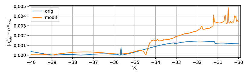
Figure 10: Distance between the fixed point of ODEs (1) and the neural network map (8) for the original and the modified systems.

The created networks not only find the fixed point location but also correctly reveal its stability properties. Figure 9(a) shows that the network correctly reproduces the bifurcation diagram for the oscillating branch of the bistability regime. It is this branch that has been showed to the network in training. But in Fig. 9(b) we observe that the second, silent branch is also discovered. This branch did not appear in the training data and recovered by the network due to its effective generalization of the training data. Observe that boundaries of the bistability area are found with very high accuracy. It means that the information about loosing stability of the fixed point is also discovered by the network. Another interesting point is that the bursting attractors for the original and for the modified systems are visually almost indistinguishable, compare Figs. 1(a,b,c) and 4(a,b,c). But nevertheless the network is able to distinguish them in the course of training: using data produced by the original system results in the neural network map with the unstable fixed point while the training data for the modified system results in the neural network map with the bistability.

Figure 9(c) shows the largest real part of the eigenvalue of the fixed point $\mu_{1}$. Similarly to Fig. 5(c) to adjust scales of positive and negative values of the eigenvalue the positive values are plotted in logarithmic scale. As expected, the areas of stability of the fixed point in Fig. 9(b) correspond to negative values of its largest eigenvalue. Observe high similarity of the curves for eigenvalues in Figs. 5(c) and 9(c) computed for ODE (1) and for the neural network map (8), respectively.

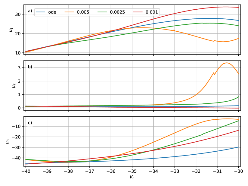
Figure 11: Eigenvalues of the fixed point of the ODEs (1) and the neural network map (8), the original system. Three networks are considered trained for $\Delta t=0.005$, $0.0025$, and $0.001$.

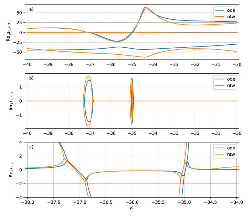
Figure 12: (a,b) Real and imaginary parts of the eigenvalues for the ODEs and the network, the modified system. (c) Real parts of the eigenvalues, enlarged area in the middle part of the panel (a).

In more details the eigenvalues of the fixed point are tested in Figs. 11 and 12. Figure 11 shows the eigenvalues computed for the original system and for the corresponding network map. The eigenvalues are real within the whole parameter range. Three neural networks are represented. In addition to the main one at $\Delta t=0.005$ we also trained two networks with smaller time steps $\Delta t=0.0025$ and $\Delta t=0.001$. Observe qualitative similarity of the eigenvalues computed for the networks with the true values computed for ODEs: all of them are real, two largest are positive for all cases. It means the trajectory leaving the vicinity of the fixed point behave in the same ways in all cases: there are two unstable directions and no rotation around it occurs since there are no imaginary parts. Eigen values for the networks coincide very well with those for ODEs in the left part of the figures and diverge in the right part. We conjecture that the spiking attractor requires finer time resolution. In favor of this assumption is the behavior of the eigenvalue curves computed for the networks trained with smaller time steps. We see that decreasing the time step results in better approximation of the true curve obtained for the ODEs.

The eigenvalues of the fixed point for the modified system with bistability is shown in Fig. 12. Panels (a) and (b) represent real and imaginary parts, respectively. Observe remarkable correspondence between the values computed for ODEs and for the network. Figure 12(c) shows two largest real parts of the eigenvalues near the area of bistability. We see that the network reproduces sufficiently fine details: the area of the negative values in the middle is bounded by segments with coinciding real parts. As one can see in Fig. 12(b) this corresponds to complex conjugated eigenvalues. Then the eigenvalues again become real and diverge from each other.

Thus we see that properties of the fixed points of the original and the modified systems are remarkably discovered by the networks regardless of the fact that they were never showed to the networks during training. It works well both for the unstable fixed point and for the bistability case. For the latter it means that it is enough to impose to the network only one branch of the bistable solution and it reveals the regime of bistability and discovers the second branch.

5 Conclusion

We created an artificial neural network that reproduces dynamics of Hodgkin-Huxley-type model represented as a stiff ODE system with two fast and one slow variables. Two versions (original and modified) of the model are considered. For the considered parameter ranges the original version has unstable fixed point and oscillating attractor that can be either bursting or spiking. The modification introduces bistability such that an area in the parameter space appears where the fixed point becomes stable and coexists with the bursting attractor.

The created network operates as a recurrent map, i.e., reproduces the dynamics as a discrete time system. This is trained as a feedforward network using standard back propagation routine on trajectory cuts sampled at random parameter values within a certain range. The network structure is developed to take into account the stiffness of the modeled system. Due to different time scales it is found to be effective to model each variable with a separate subnetwork. The subnetworks have identical structures and contain three fully connected layers. The first one injects the parameter values as well as non-modeled variables. The output of this layer is added to a vector of weights of the modeled variable and the result passes trough two another layers. Scalar outputs of each subnetwork are concatenated to form a vector of dynamical variables at new time step.

Although the network is trained only on oscillatory trajectory cuts, the resulting recurrent map also acquires the fixed point whose position and even the eigenvalues coincide well with the fixed point of the initial system. In particular it means that when a bistable regime is modeled, the network being fed by only one brunch of solutions discovers another brunch, never seen in the course of training. It indicate the ability of the created network to perform proper generalization of the training data.

The obtained results, i.e., the ability of the created artificial neural network to reproduce dynamics including dynamical features never seen in the course of training are able, as we see it, to trigger new approaches to complex dynamics reconstruction problem. Potentially the methods of analysis can be developed where neural network discovers previously unknown dynamical features of the analyzed system. From the practical point of view reproducing dynamics with the neural network can be considered as a sort of alternative method of numerical modeling intended for use with contemporary parallel hard- and software. In particular it is suitable for so called AI accelerators, a hardware dedicated to deal with artificial neural networks.

Declaration of competing interest

The authors declare that they have no known competing financial interests or personal relationships that could have appeared to influence the work reported in this paper.

References

- [1] E. Levin, R. Gewirtzman, G. F. Inbar, Neural network architecture for adaptive system modeling and control, Neural Networks 4 (2) (1991) 185–191. doi:10.1016/0893-6080(91)90003-N.
- [2] B. Grieger, M. Latif, Reconstruction of the El Niño attractor with neural networks, Climate Dynamics 10 (6) (1994) 267–276. doi:10.1007/BF00228027.
- [3] H. G. Zimmermann, R. Neuneier, Combining state space reconstruction and forecasting by neural networks, in: G. Bol, G. Nakhaeizadeh, K.-H. Vollmer (Eds.), Datamining und Computational Finance, Physica-Verlag HD, Heidelberg, 2000, pp. 259–267. doi:10.1007/978-3-642-57656-0\_13.
- [4] S. Tronci, M. Giona, R. Baratti, Reconstruction of chaotic time series by neural models: a case study, Neurocomputing 55 (3) (2003) 581–591, evolving Solution with Neural Networks. doi:10.1016/S0925-2312(03)00394-1.
- [5] Z. Wang, C. Guet, Reconstructing a dynamical system and forecasting time series by self-consistent deep learning, arXiv:2108.01862 [cs.LG] (2021). arXiv:2108.01862.
- [6] A. N. Kolmogorov, On the representation of continuous functions of several variables by superpositions of continuous functions of a smaller number of variables, Doklady Akademii Nauk SSSR 108 (1956) 179–182, english translation: Amer. Math. Soc. Transl., 17 (1961), pp. 369-373.
- [7] A. N. Kolmogorov, On the representation of continuous functions of many variables by superposition of continuous functions of one variable and addition, Doklady Akademii Nauk SSSR 114 (1957) 953–956, english translation: Amer. Math. Soc. Transl., 28 (1963), pp. 55–59.
- [8] V. I. Arnold, On functions of three variables, Doklady Akademii Nauk SSSR 114 (1957) 679–681, english translation: Amer. Math. Soc. Transl., 28 (1963), pp. 51–54.
- [9] G. Cybenko, Approximation by superpositions of a sigmoidal function, Mathematics of Control, Signals and Systems 2 (4) (1989) 303–314. doi:10.1007/BF02551274.
- [10] S. Haykin, Neural networks and learning machines, 3rd Edition, Pearson Prentice Hall, 2009.
- [11] N. P. Jouppi, C. Young, N. Patil, D. Patterson, G. Agrawal, R. Bajwa, S. Bates, S. Bhatia, N. Boden, A. Borchers, R. Boyle, P.-l. Cantin, C. Chao, C. Clark, J. Coriell, M. Daley, M. Dau, J. Dean, B. Gelb, T. V. Ghaemmaghami, R. Gottipati, W. Gulland, R. Hagmann, C. R. Ho, D. Hogberg, J. Hu, R. Hundt, D. Hurt, J. Ibarz, A. Jaffey, A. Jaworski, A. Kaplan, H. Khaitan, D. Killebrew, A. Koch, N. Kumar, S. Lacy, J. Laudon, J. Law, D. Le, C. Leary, Z. Liu, K. Lucke, A. Lundin, G. MacKean, A. Maggiore, M. Mahony, K. Miller, R. Nagarajan, R. Narayanaswami, R. Ni, K. Nix, T. Norrie, M. Omernick, N. Penukonda, A. Phelps, J. Ross, M. Ross, A. Salek, E. Samadiani, C. Severn, G. Sizikov, M. Snelham, J. Souter, D. Steinberg, A. Swing, M. Tan, G. Thorson, B. Tian, H. Toma, E. Tuttle, V. Vasudevan, R. Walter, W. Wang, E. Wilcox, D. H. Yoon, In-datacenter performance analysis of a tensor processing unit, SIGARCH Comput. Archit. News 45 (2) (2017) 1–12. doi:10.1145/3140659.3080246.
- [12] J. Welser, J. W. Pitera, C. Goldberg, Future computing hardware for AI, in: 2018 IEEE International Electron Devices Meeting (IEDM), 2018, pp. 131–136. doi:10.1109/IEDM.2018.8614482.
- [13] K. Karras, E. Pallis, G. Mastorakis, Y. Nikoloudakis, J. M. Batalla, C. X. Mavromoustakis, E. Markakis, A hardware acceleration platform for AI-based inference at the edge, Circuits, Systems, and Signal Processing 39 (2) (2020) 1059–1070. doi:10.1007/s00034-019-01226-7.
- [14] P. V. Kuptsov, A. V. Kuptsova, N. V. Stankevich, Artificial neural network as a universal model of nonlinear dynamical systems, Russian Journal of Nonlinear Dynamics 17 (1) (2021) 5–21. doi:10.20537/nd210102.
- [15] A. Sherman, J. Rinzel, J. Keizer, Emergence of organized bursting in clusters of pancreatic beta-cells by channel sharing, Biophysical Journal 54 (3) (1988) 411–425. doi:10.1016/S0006-3495(88)82975-8.
- [16] L.-W. Kong, H.-W. Fan, C. Grebogi, Y.-C. Lai, Machine learning prediction of critical transition and system collapse, Phys. Rev. Research 3 (2021) 013090. doi:10.1103/PhysRevResearch.3.013090.
- [17] L.-W. Kong, H. Fan, C. Grebogi, Y.-C. Lai, Emergence of transient chaos and intermittency in machine learning, Journal of Physics: Complexity 2 (3) (2021) 035014. doi:10.1088/2632-072x/ac0b00.
- [18] B. Thorne, T. Jüngling, M. Small, D. Corrêa, A. Zaitouny, Reservoir time series analysis: Using the response of complex dynamical systems as a universal indicator of change, Chaos: An Interdisciplinary Journal of Nonlinear Science 32 (3) (2022) 033109. doi:10.1063/5.0082122.
- [19] N. Stankevich, E. Mosekilde, Coexistence between silent and bursting states in a biophysical Hodgkin-Huxley-type of model, Chaos: An Interdisciplinary Journal of Nonlinear Science 27 (12) (2017) 123101. doi:10.1063/1.4986401.
- [20] I. Goodfellow, Y. Bengio, A. Courville, Deep learning (adaptive computation and machine learning series), Cambridge Massachusetts (2017) 321–359.
- [21] D. P. Kingma, J. Ba, Adam: A method for stochastic optimization, arXiv:1412.6980 [cs.LG], published as a conference paper at International Conference on Learning Representations (ICLR) 2015 (2014). arXiv:1412.6980.