Energy cost of dynamical stabilization: stored versus dissipated energy

Abstract

Dynamical stabilization processes (homeostasis) are ubiquitous in nature, but energetic resources needed for their existence were not studied systematically. Here we undertake such a study using the famous model of Kapitza’s pendulum, which attracted attention in the context of classical and quantum control. This model is generalized, made autonomous, and we show that friction and stored energy stabilize the upper (normally unstable) state of the pendulum. The upper state can be made asymptotically stable and yet it does not cost any constant dissipation of energy, only a transient energy dissipation is needed. The asymptotic stability under a single perturbation does not imply stability with respect to multiple perturbations. For a range of pendulum-controller interactions, there is also a regime where constant energy dissipation is needed for stabilization. Several mechanisms are studied for the decay of dynamically stabilized states.

I Introduction

Dynamical stabilization is an important concept in physics (particle trapping, Floquet engineering) paul ; cook ; fish ; polko , control theory (vibrational stabilization and robotics) mech_1 ; mech_2 ; control ; ieee , biology (homeostasis) review ; billman ; soodak ; novo , animal locomotion animal ; animal_2 , and population dynamics (polymorphism in time-dependent environment) arm1 ; arm2 . The meaning of this concept is that certain relevant parameters (concentrations, coordinates) are stabilized against external perturbations by active and frequently self-regulating means. This is achieved via specific engines or controllers, and no stability will exist without their action.

Is there an energy cost for dynamic stabilization and how it is to be estimated? This question is of obvious relevance for controlling methods. A general explanation for homeostasis in biology is that it offers energetically cheaper realizations of physiological functions review . This makes relevant to ask about its own energy costs.

In order to study the energy cost problem, we chose a simple but non-trivial model that exhibits dynamical stabilization. This is the driven non-linear pendulum, whose upper (normally unstable state) can be stabilized by a sufficiently fast external force thereby defying gravity. Such models were first studied by Stephenon steph , and then by Kapitza kapitza ; LL ; see butikov for a review. They still produce new physical results acheson ; blackburn ; fishman and have interesting applications paul ; cook ; fish ; polko ; mech_1 ; mech_2 ; animal ; animal_2 ; control ; ieee .

Our first step will be to replace the external field with a controller degree of freedom in order to make the driven pendulum autonomous. This ensures finite energies and accounts of all relevant degrees of freedom; see section II. The autonomous pendulum predicts the following two scenarios for dynamical stabilization of the unstable state. Within the first scenario, the state is asymptotically stable. There are two factors behind this strong notion of stabilization: the energy stored in the controller that ensures the needed effective potential, and the friction acting on the pendulum. (Obviously, friction is necessary for asymptotic stability.) There are no permanent energy costs here, i.e. once the asymptotically stable state is reached, the interaction with the controller is automatically switched off. There is only a moderate transient dissipation of energy during relaxation. The interaction emerges on-line together with an external perturbation.

However, the notion of asymptotic stability is not sufficient for characterizing this scenario of dynamic stabilization. Contrary to passively stabilized systems, asymptotic stability does not guarantee stability under a sequence of well-separated perturbations acting within the attraction basin. For characterizing this more general notion of stability we again need the concept of stored energy.

The second scenario predicted by the model is realized when the back-reaction from pendulum to controller is sizable. Here the the asymptotic stability is replaced by a metastable stabilization that has a finite (though possibly long) life-time, because the controller steadily dissipates the stored energy for supporting the metastable state. Once this energy is lower than a certain threshold, the metastable state suddenly decays with dissipating away all the energy. Therefore, dynamic stabilization within this scenario requires permanent energy costs.

Thus, the model provides conceptual tools and scenarios for addressing the energy cost problem in more general (especially biological) dynamic stabilization situations.

This paper is organized as follows. The generalized Kapitza’s model is formulated in section II, and is approximately solved in section III. We show that the asymptotic stability of the inverted pendulum is determined (among other factors) by the energy stored in the controller. This extends the stability criterion presented in kapitza ; LL ; butikov . In section IV we confirm the analytic bound, and work out numerically two basic scenarios of dynamic stability. Section IV.2 discusses a new scenario of noise-induced metastability. Our results are summarized in the last section, where we also discuss possible biological implications of our research.

II Pendulum and controller

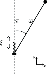
Figure 1: A schematic representation of the inverted pendulum. The angle $\varphi$ is defined such that the upper (normally unstable) position refers to $\varphi=\pi$. The end-point of the pendulum moves vertically with coordinate $\xi$ that is subject to a harmonic potential; cf. (3).

As a result of its numerous applications, Kapitza’s pendulum can be introduced in a variety of contexts. For clarity, we shall introduce its generalization within a mechanical picture; cf. LL . Consider a pendulum moving on $(x,y)$ plane in a homogeneous gravity field $g$; see Fig. 1. The pendulum is a material point with mass $m$ fixed at one end of a rigid rod with length $l$. Let the coordinates and velocities of the mass be

$$x=l\sin\varphi,\quad\dot{x}\equiv\frac{{\rm d}x}{{\rm d}t}=l\cos\varphi\cdot\dot{\varphi},$$ (1)

$$y=\xi_{0}-l\cos\varphi,\quad\dot{y}\equiv\frac{{\rm d}y}{{\rm d}t}=\dot{\xi}_{0}+l\sin\varphi\cdot\dot{\varphi},$$ (2)

where $\xi_{0}$ refers to vertical (along $y$-axes) motion of the opposite end of the road. The Lagrangian of the autonomous system with coordinates $(x,y,\xi)$ reads

$$L=\frac{m}{2}[\dot{x}^{2}+\dot{y}^{2}]-mgy+\frac{\mu}{2}\dot{\xi}_{0}^{2}-\frac{k}{2}{\xi}_{0}^{2},$$ (3)

where $\mu$ is the mass of $\xi_{0}$, and we assumed a harmonic potential $\frac{k}{2}{\xi}_{0}^{2}$ for $\xi_{0}$. Putting (1, 2) into (3), denoting $\xi=\xi_{0}+\frac{mg}{k}$, and dropping a constant term from Lagrangian we find

$$L=\frac{ml^{2}}{2}\dot{\varphi}^{2}+\frac{\mu+m}{2}\dot{\xi}^{2}+ml\dot{\xi}\dot{\varphi}\sin\varphi+mgl\cos\varphi-\frac{k}{2}{\xi}^{2},$$ (4)

which implies Lagrangian equations of motion $\frac{{\rm d}}{{\rm d}t}\frac{\partial L}{\partial\dot{q}}=\frac{\partial L}{\partial q}$ with coordinates $q=(\varphi,\xi)$ and velocities $\dot{q}=(\dot{\varphi},\dot{\xi})$:

$$\ddot{\varphi}+\frac{g}{l}\sin\varphi=-\frac{1}{l}\sin\varphi\cdot\ddot{\xi},$$ (5)

$$\ddot{\xi}+\omega^{2}\xi=-\epsilon\;[\;\cos\varphi\cdot{\dot{\varphi}}^{2}+\sin\varphi\cdot\ddot{\varphi}\;],$$ (6)

$$\omega^{2}\equiv{k}/({\mu+m}),\qquad\epsilon\equiv{l}/({1+\frac{\mu}{m}}),$$ (7)

where $\omega$ is the frequency of $\xi$, while $\epsilon$ characterizes the back-reaction of $x$ on $\xi$. Note from (3, 6) that whenever $\mu\gg m$, i.e. the controller $\xi$ is much heavier than the pendulum, we can neglect the left-hand-side of (6), and revert to the usual (non-autonomous) driven pendulum. This, however, does not suffice for the full understanding of energy costs, which arise due to the very back-reaction of $x$ on $\xi$.

Eqs. (5, 6) are deduced from the time-independent Lagrangian (4); hence they are conservative and reversible. The conserved energy related to (4) reads:

$$E=\dot{\varphi}\frac{\partial L}{\partial\dot{\varphi}}+\dot{\xi}\frac{\partial L}{\partial\dot{\xi}}-L=\frac{ml^{2}}{2}\dot{\varphi}^{2}+\frac{\mu+m}{2}\dot{\xi}^{2}+ml\dot{\xi}\dot{\varphi}\sin\varphi-mgl\cos\varphi+\frac{k}{2}{\xi}^{2}.$$ (8)

We shall now add a friction with parameter $\gamma>0$ to (5) writing it as

$$\ddot{\varphi}+\frac{g}{l}\sin\varphi+\gamma\dot{\varphi}=-\frac{1}{l}\sin\varphi\cdot\ddot{\xi}.$$ (9)

As seen below, this friction is a means of stabilizing the motion of $\varphi$. We do not add a friction to the controller degree of freedom $\xi$, since this will reach no constructive goal besides providing an additional channel for loosing energy. We shall also mostly neglect random noises acting on $\varphi$, i.e. we do not study Langevin equations. The influence of a random noise is discussed in section IV.2.

Note that energy (8) governed by (6, 9) decays in time as it should:

$$\frac{{\rm d}E}{{\rm d}t}=-ml^{2}\gamma\dot{\varphi}^{2}\leq 0.$$ (10)

As confirmed below, it is useful to separate the energy $E$ in (8) into two contributions, those descrbing the motion of $\xi$ and $\varphi$:

$$E=E_{\varphi}+E_{\xi},\qquad E_{\xi}=\frac{\mu+m}{2}\dot{\xi}^{2}+\frac{k}{2}{\xi}^{2}.$$ (11)

III Solving the model via slow and fast variables

To solve non-linear (6, 9), we shall apply both separation of time-scales and perturbation theory. We assume that $\omega$ in (6) is a large parameter, i.e. $\xi$ oscillates fast. Next, we separate $\varphi$ as LL :

$$\varphi=\Phi+\zeta,\qquad\zeta\ll\Phi$$ (12)

where $\Phi$ is slow and $\zeta$ is fast, and also small compared with $\Phi$. Then from (6, 9, 12) we get after expanding over $\zeta$ and keeping the first non-vanishing term only:

$$\ddot{\Phi}+\ddot{\zeta}+\frac{g}{l}\sin\Phi+\zeta\frac{g}{l}\cos\Phi+\gamma\dot{\Phi}+\gamma\dot{\zeta}=-\frac{1}{l}\sin\Phi\cdot\ddot{\xi}-\frac{1}{l}\cos\Phi\cdot\zeta\ddot{\xi},$$ (13)

$$\ddot{\xi}+\omega^{2}\xi=-\epsilon[(\cos\Phi-\zeta\sin\Phi)(\dot{\Phi}+\dot{\zeta})^{2}+(\sin\Phi+\zeta\cos\Phi)(\ddot{\Phi}+\ddot{\zeta})].$$ (14)

Assuming that $\gamma\gtrsim\frac{1}{\omega}$, and noting that for fast variables $\dot{\zeta}$, $\ddot{\zeta}$, $\dot{\xi}$, and $\ddot{\xi}$ are big, we can equalize fast and big components in (13, 14):

$$\ddot{\zeta}+\gamma\,\dot{\zeta}=-\frac{1}{l}\sin\Phi\cdot\ddot{\xi},$$ (15)

$$\ddot{\xi}+\omega^{2}\xi=-\epsilon\sin\Phi\cdot\ddot{\zeta},$$ (16)

$$\zeta(0)=0,$$ (17)

where initial condition (17) is imposed without loss of generality; cf. (12). In (16) we, in particular, neglected the factor $-\epsilon\cos\Phi\cdot\dot{\zeta}^{2}$, because it is quadratic over $\zeta$. Note that (15, 16) do not contain the contribution $\zeta\frac{g}{l}\cos\Phi$ coming from the potential $-mgl\cos\varphi$ [cf. (13)], since this contribution is not sufficiently fast, i.e. (15, 16) involve only time-derivatives of $\zeta$.

Eq. (15) can be integrated over the time. A constant of integration should be put to zero, since $\zeta$ and $\dot{\xi}$ are oscillating in time with their time-average being zero. Hence the integration of (15) implies

$$\dot{\zeta}(0)=-\frac{\sin\Phi}{l}\dot{\xi}(0).$$ (18)

Eqs. (15, 16) are linear over the unknown variables $\zeta$ and $\psi$, and they can be solved via the Laplace transform [see Appendix]. Now we can average (13) over fast oscillations:

$$\ddot{\Phi}+\frac{g}{l}\sin\Phi+\gamma\dot{\Phi}+\frac{1}{l}\cos\Phi\cdot\overline{\zeta(t)\,\ddot{\xi}(t)}=0,$$ (19)

where $\overline{...}$ means time-averaging over fast oscillations. The factor $\overline{\zeta(t)\,\ddot{\xi}(t)}$ in (19) is worked out in Appendix. It does contribute to an effective (generally time-dependent) potential $\Pi(\Phi)$:

$$\ddot{\Phi}+\gamma\dot{\Phi}=-\partial_{\Phi}\Pi(\Phi).$$ (20)

The form of this potential simplifies if we assume that a slow variable $\beta\equiv\frac{\sin^{2}\Phi}{1+\frac{\mu}{m}}$ holds $\beta\ll 1$ due to $\frac{\mu}{m}\gg 1$ (weak back-reaction), and take the first non-vanishing term over $\beta$; see Appendix. This approximation is only supported when the slow variable $\Phi$ relaxes to $\pi$ or to $0$. Eventually, we have a simplified form of the effective potential:

$$\Pi=-\frac{g}{l}\cos\Phi-\frac{\omega^{2}}{\gamma^{2}+\omega^{2}}\cdot\frac{\dot{\xi}^{2}(0)+\omega^{2}\xi^{2}(0)}{8l^{2}}\cdot\cos 2\Phi.$$ (21)

Now $\Phi=\pi$ is stable, i.e. $\partial_{\Phi}\Pi(\Phi)|_{\Phi=\pi}=0$ and $\partial^{2}_{\Phi}\Pi(\Phi)|_{\Phi=\pi}>0$, if:

$$\frac{\dot{\xi}^{2}(0)+\omega^{2}\xi^{2}(0)}{2gl}>1+\frac{\gamma^{2}}{\omega^{2}}.$$ (22)

Note that larger values of $\omega$ expectedly increase the stability domain. However, larger values of the friction constant $\gamma$ decrease it. Hence, the friction plays a double role in this system, since the very relaxation of $\Phi(t)$ (e.g. $\Phi(t)\to\pi$) is achieved due to friction .

Eqs. (20, 21) imply that when $\Phi=\pi$ is a stable rest point, we get that the slow part $\Phi(t)$ of the angle variable $\varphi(t)$ convergence due to the friction: $\Phi(t)\to\pi$, if $\Phi(0)$ is in the attraction basin of $\Phi=\pi$. What happens then to the fast part $\zeta(t)$ of $\varphi(t)$? This is a convoluted question that we clarify below numerically. Our results in Appendix show that when the derivation (12–18) applies—i.e. both the time-scale separation and the perturbation over $\beta$ hold—we get $\zeta(t)\to 0$ together with $\Phi(t)\to\pi$; see (28). This is indeed observed numerically, as seen below. However, there is also a regime that is not described by (12–18), where $\Phi(t)\to\pi$ for sufficiently long, but finite times, and where $\zeta(t)$ stays non-zero; see below for details. This regime is realized when the back-reaction parameter $\epsilon$ is sufficiently large. As we emphasized, the above analytic derivations do not hold for this case. Eventually, the fact of large back-reaction leads to decaying of the $\Phi=\pi$ state, i.e. $\Phi=\pi$ turns out to be a metastable state.

Finally, note that the left-hand-side of (22) is just the initial dimensionless energy of $\xi$; cf. (7, 11). We call this quantity the initial stored energy and remind again that (22) was obtained for vanishing back-reaction $\epsilon\to 0$.

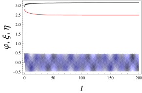
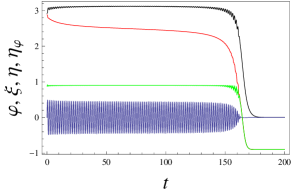
Figure 2: (a) This figure shows the angle variable $\varphi$ (black, upper curve) and the controller $\xi$ (blue, oscillating curve) as numerical solutions of (6, 9) versus time $t$. The red curve (in the middle) is the scaled energy $\eta=\frac{E}{\mu+m}$ that includes the stored energy $\frac{1}{2}[\dot{\xi}^{2}+\omega^{2}\xi^{2}]$; cf. (8, 22). Parameters in (6, 9) are: $\epsilon=0.8$, $\dot{\xi}(0)=2$ ($\xi(0)=0$), $\varphi(0)=0.93\pi$ ($\dot{\varphi}(0)=0$), $\omega=4$, $\gamma=3$, $m=g=l=1$.
It is seen that $\varphi$ quickly stabilizes at $\varphi=\pi$, which is normally an unstable state. The stabilization process takes a relatively small amount of energy. After the stabilization $\varphi$ and $\xi$ decouple; $\xi$ continues oscillating, and the scaled energy $\eta$ is then constant in time. The stability condition (22) holds. (The difference between its LHS and RHS is $0.4375$.)
(b) The same parameters as in (a), but now the backreaction parameter $\epsilon=0.9$ is slightly larger. We also display $\eta_{\varphi}=\frac{E}{\mu+m}-\frac{1}{2}\dot{\xi}^{2}-\frac{\omega^{2}}{2}{\xi}^{2}$ (green curve, third from top), where $\eta_{\varphi}$ is the (scaled) energy related to the angle variable only; cf. (8). Now there is rather long ($t\sim 150$) period of metastability, accompanied by a slow dissipation of energy. After this the stability is lost: $\varphi$ quickly relaxes to the minimum $\varphi=0$ of the potential, $\xi$ looses all its energy and eventually stops moving (i.e. $\xi(t)\to 0$). The whole stored energy is dissipated away.
The physical reason of scenario in (b) is that fast oscillations around $\varphi=\pi$ do not disappear, i.e. they persist in the metastable state, continuously dissipate energy [cf. (10)], and once the initial energy decreases sufficiently, the $\varphi$ and $\xi$ (relatively) suddenly move to the global energy minimima $\varphi=\dot{\varphi}=\xi=\dot{\xi}=0$. We emphasize that it is the energy $\frac{1}{2}\dot{\xi}^{2}+\frac{\omega^{2}}{2}{\xi}^{2}$ stored in $\xi$ that decays in time. To confirm this, (b) also shows the scaled energy $\zeta_{\varphi}$ related to $\varphi$. It stays constant in time for the whole metastability period; see the green curve. A similar scenario happens, when the initial condition $\varphi(0)$ is out of the attraction basin of $\varphi=\pi$. However, here $\varphi(t)$ never reaches $\pi$.

IV Scenarios of (de)stabilization for the inverted pendulum

IV.1 Asymptotic stability and stability with respect to several perturbations

Fig. 2 shows solution of (6, 9) when condition (22) holds. It is seen that indeed the state $\varphi=\pi$ gets asymptotically stabilized, $\varphi(t)\to\pi$ at least when $\Phi(0)$ is sufficiently close to $\pi$, i.e. when $\varphi(0)$ is in the attraction basin of $\pi$. This relaxation is accompanied by the energy dissipation. The decaying (dissipating) quantity here is mostly the stored energy $\frac{1}{2gl}[\dot{\xi}^{2}(t)+\omega^{2}\xi^{2}(t)]$, i.e. the dimensionless energy related to $E_{\xi}$ in (11). Once $\varphi$ approaches $\pi$ sufficiently close, the coupling between $\xi$ and $\varphi$ is switched off; recall the discussion after (22). This means that the stored energy is not anymore dissipated and stays constant for subsequent times; see Fig. 2. Thus, we confirm that the originally unstable fixed point of the pendulum can be made asymptotically stable without permanent energy costs, but with a transient energy dissipation only.

For parameters of Fig. 2 the point $\varphi=\pi$ is asymptotically stable with a well-defined attraction basin; i.e. it is stable with respect to a single perturbation, which refers to the initial state $\varphi(0)=0.93\pi$, $\dot{\varphi}(0)=0$, and specific initial state $(\xi(0),\dot{\xi}(0))$ of $\xi$; see Fig. 2. It is necessary to generalize the notion of asymptotic stability, because it is unrealistic to consider only a single perturbation. Let us assume that after $\varphi(t)$ relaxed to $\pi$, we apply at some random time $\tau$ (which is larger than the relaxation time) yet another (second) perturbation $\varphi=\pi\to\varphi(0)=\varphi(\tau)$ within the same attraction basin, i.e. $\varphi(0)=0.93$ for parameters of Fig. 2. The initial state of $\xi$ is then reset as $(\xi(\tau),\dot{\xi}(\tau))$. Hence we now run the dynamics anew with initial states $\varphi(0)=0.93\pi$, $\dot{\varphi}(0)=0$, $\xi(\tau)$ and $\dot{\xi}(\tau)$.

It appears that for parameters of Fig. 2, $\varphi=\pi$ is unstable after the second perturbation. The issue here is that the back-reaction $\epsilon$ is sufficiently large, hence the second perturbation alters the controlling degree of freedom $\xi(t)$ and also dries out its stored energy, which already decreased after the first perturbation. If for parameters of Fig. 2 we decrease $\epsilon$ from $0.8$ to $0.1$, $\varphi$ becomes stable to many well-separated (in the above sense) perturbations coming at random times. One reason for this is that the stored energy decrease within one perturbation is smaller. Another reason, which numerically clearly differs from the first one, is that the motion of $\xi$ becomes more stable with respect to resetting the initial conditions of $\varphi$ during the perturbation.

IV.2 Random noise

Above we assumed multiple, strong and well-separated (in time) perturbation. Another way of implementing multiple perturbations is to include an external noise in (9). Let us add to the right-hand-side of (9) a white, Gaussian random noise:

$$\sigma f(t),\qquad\langle f(t)\rangle=0,\quad\langle f(t)f(t^{\prime})\rangle=\delta(t-t^{\prime}),$$ (23)

where $\sigma$ is the noise intensity. The modified (9) becomes then the Langevin equation (for $\varphi(t)$). In contrast to strong and well-separated (in time) perturbations, (23) allows uncorrelated, densely located perturbations that are (most probably) weak if $\sigma$ is small.

Now Fig. 3 shows that a weak-random noise monotonously dries out the stored energy, and hence the stability of $\varphi=\pi$ is lost after a sufficiently long time. Fig. 3 shows that the same scenario hold for a stronger noise, though in somewhat blurred form and for a shorter life-time of the metastable state. For parameters of Fig. 3 and $\sigma=0$, $\varphi=\pi$ is asymptotically stable with respect to $10-11$ strong, well-separated perturbations.

This metastability under noise differs from the well-known noise-induced escape from a local energy minimum to a deeper minimum. There a sufficiently strong random kick brings the system to the attraction basin of the deeper minimum. In contrast, here the attraction basin is not changed (and no strong kicks are to be waited for). Rather the stored energy needed for maintaining the stability is drained out and the very local minimum state is destroyed. Hence, what we described here constitutes a new type of noise-induced metastability that deserves further study.

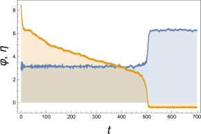
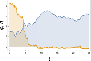
Figure 3: (a) The angle $\varphi$ (blue, piece-wise constant curve) as the numerical solution of (6, 9) versus time $t$, where to the RHS of (9) we added an addtive white noise $f(t)$ with intensity $\sigma=0.1$; see (23). Here $\eta=\frac{E}{\mu+m}$ (orange, decaying curve) is the scaled energy; cf. (8). Parameters in (6, 9) are: $\epsilon=0.4$, $\dot{\xi}(0)=4$ ($\xi(0)=0$), $\varphi(0)=0.93\pi$ ($\dot{\varphi}(0)=0$), $\omega=4$, $\gamma=3$, $m=g=l=1$.
It is seen that $\phi$ is stabilized around $\pi$ in a metastable state whose life-time is $\simeq 500$. During this life-time the energy $\eta$ slowly decays, till it is below some critical value, and then the metastable state suddenly decays.
(b) The same as in (a), but for a stronger noise $\sigma=1.25$. Metastable decay is smeared, but still clearly visible.

IV.3 Metastability

For parameters of Fig. 2, if the back-reaction $\epsilon$ is larger than $0.8$ another interesting scenario takes place: the notion of asymptotic stability with respect a single perturbation is lost and is replaced by metastability; see Fig. 2.

Now small oscillations of $\varphi(t)$ around $\Phi=\pi$ persist and do not decay in time; cf. (12). According to (10), these oscillations slowly drain out the initial stored energy $\frac{1}{2gl}[\dot{\xi}^{2}(0)+\omega^{2}\xi^{2}(0)]$, and when it gets sufficiently low, the metastable state $\Phi=\pi$ suddenly decays to the global energy minimum $\varphi=\dot{\varphi}=\xi=\dot{\xi}=0$; see Fig. 2. During this sudden decay the whole stored energy is dissipated away. Note that in the metastability time-window the energy $E_{\varphi}$ related to $\varphi$ stays constant; see (11) and Fig. 2.

The transition between regimes in Fig. 2 and Fig. 2, i.e. between the truly stable and the metastable state takes place for a critical value of the backreaction parameter $\epsilon_{c}$. For parameters of Fig. 2 and 2 we have $\epsilon_{c}\approx 0.86075$. We checked numerically that the life-time of the metastable state can be very large for $\epsilon$ approaching $\epsilon_{c}$ from above. Hence we conjecture that this time can be arbitrary large for $\epsilon\to\epsilon_{c}+0$.

We emphasize that the transition between regimes in Fig. 2 and Fig. 2 is described for fixed initial conditions of $\varphi$: $\varphi(0)=0.93\pi$ ($\dot{\varphi}(0)=0$), i.e. for a fixed attraction basin of the stabilized state. If these initial conditions are changed by making $\varphi(0)$ closer to the stability point $\pi$ (i.e. the attraction basin is shrunk), then the transition from the stable to metastable regime takes place at a larger value of $\epsilon$, or does not take place at all. Likewise, if the attraction basin is enlarged, the transition taken place for smaller $\epsilon$. For example, if $\varphi(0)=0.92\pi$ ($\dot{\varphi}(0)=0$), then the transition takes place at $\epsilon_{c}\simeq 0.6536$, while for $\varphi(0)=0.935\pi$ ($\dot{\varphi}(0)=0$), the solution is stable for all $\epsilon<1$, which is the physical range of $\epsilon$ for parameters of Fig. 2 and Fig. 2; cf. (7). Note that the stabilization with the largest attraction basin demands vanishing values of $\epsilon$. In particular, for parameters of Fig. 2, no stabilization of the $\varphi=\pi$ state occurs for $|\varphi(0)|<0.64105\pi$ ($\dot{\varphi}(0)=0$), while for $|\varphi(0)|\gtrsim 0.64105\pi$ the stabilization demands $\epsilon\to 0$.

Note that the metastability in Figs. 3 and 3 is different from that in Fig. 2, because in the latter case the metastability is due to a strong back-reaction, and not permanently acting perturbations.

V Summary and Discussion

The purpose of this work is to understand energy costs of dynamical stabilization (homeostasis): a process that stabilizes an unstable state due to an active controlling process. To this end, one needs plausible models with a well-established history of physical paul ; cook ; fish ; polko ; steph ; kapitza ; LL ; butikov ; acheson ; blackburn ; fishman and control-theoretic mech_1 ; mech_2 ; animal ; animal_2 ; control ; ieee applications. Here we studied the inverted (Kapitza’s) pendulum model, where the upper (normally unstable) state is stabilized by a fast motion of a controlling degrees of freedom. Usually, this degree of freedom is replaced by an external field. But here we modeled it explicitly, because we want to study an autonomous system with a full control of energy and its dissipation. Our main results are summarized as follows.

The unstable state of the pendulum can be asymptotically stabilized—with a finite attraction basin—without permanent energy dissipation, because the controller-pendulum interaction is automatically switched off once the pendulum is stabilized. Here there is only a transient dissipation of a small amount of energy related to the stabilization. This regime is reached when both the backreaction of the pendulum to the controller is sufficiently small and the controller oscillates sufficiently fast, i.e. it does have a sizable stored energy.

However, the notion of asymptotic stability is not sufficient: we need to study stability with respect to multiple perturbations. We implemented two scenarios for multiple perturbations: strong, widely separated in time perturbations, and a weak white noise acting on the pendulum. An asymptotically stable state may not be stable with respect to several perturbations. The latter type of stability is achieved only if the back-reaction to the controller is small. In the second scenario, a weak white noise leads to a noise-driven decay of a metastable state. This decay differs in several ways from the usual noise-driven escape. There is a need for further, more systematic research on this effect.

When the back-reaction is larger, the very notion of asymptotic stability is lost and is replaced by metastability. Now the stabilization is temporary (metastable), because small oscillations around the stabilized state do not decay. They dry out the stored energy of the controller, and once it is lower than some threshold the metastable state decays. In this case, we do get that a constant dissipation rate is needed for supporting the metastable state.

Note that the energy cost problem was actively studied for the case of adaptation gorban . Here the stability is required with respect to external changes of intensive variables; e.g. temperature, chemical potential etc sartori_nature ; wang ; sartori_prl ; prl ; gorban . Adaptation should be distinguished from the proper dynamical stabilization (homeostasis) c_gorban . Adaptation is about stability of intensive variables (e.g. temperature). It relates to structural changes in the system, while the homeostasis need not. Hence, adaptation is thermodynamically restricted by the Le Chatelier-Braun principle, whereas homeostasis is not wang ; c_gorban ; gilmore . The existing approaches to energy cost of adaptation show that the energy is to be dissipated continuously if an adaptive state is maintained sartori_nature ; wang ; sartori_prl ; prl . In that sense adaptation is similar to proof-reading and motor transport, biological processes that are essentially non-equilibrium and demand constant dissipation of energy; see jsp for a review. The question of relating dynamical stabilization and adaptation more directly remains open; so far, the two concepts have been quite separate.

Conceptual tools gained from the physical model should be useful for studying the energy cost of biological examples of dynamical stabilization (homeostasis) review ; billman ; soodak ; novo . Biological and physiological discussions imply that homeostasis is needed for controlling (and providing advantages for) metabolic processes in organisms review ; billman ; soodak ; novo . This makes necessary to ask about the proper energy costs of the homeostasis itself. Such costs can be substantial, e.g. humming birds (colibri)—for which energy saving is crucial—fall at night into a torpor state that is different from the normal sleep. In this state several homeostatic mechanisms—including internal energy regulation—are ceased. Thereby birds are able to save a substantial amount of energy: up $\simeq 60\%$ of the normal usage colibri .

Since realistic models of homeostasis are derived from systems biology review ; gorban , they frequently lack a physical form that allows us to ask questions about energy balance, let alone its dissipation. Nonetheless, some analogies can be drawn and might prove useful in future research. We saw that the energy stored in the controlling degree of freedom can be the main resource of homeostasis. In that respect it is similar to the energy stored in the living organism, one of major concepts in biological thermodynamics bauer ; mcclare ; jaynes ; blumenfeld ; arshav ; debt1 ; debt2 . It also relates to adaptation energy introduced in physiology gorban ; cf. c_gorban for a critical discussion. The stored energy is phenomenologically employed in Dynamic Energy Budget Theory (DEBT) debt1 ; debt2 and applied for estimating metabolic flows of concrete organisms.

This concept is not yet well-formalized, but some of its qualitative features are known. The stored energy is not the usual free energy, since the latter is present in equilibrium as well. From the viewpoint of a modern thermodynamics, the notion of the stored energy resembles the energy kept at certain negative temperature, because it is capable of doing work in a cyclic process balian . Now for the inverted pendulum the stored energy is mechanical (not chemical) and relates to an oscillating degree of freedom, but it is also capable of doing a cyclic work. The inverted pendulum does demonstrates how stored energy relates to stabilizing unstable states.

Appendix A Solution of Eqs. (15, 16)

Define from (7)

$$\beta\equiv\frac{\epsilon\,\sin^{2}\Phi}{l}=\frac{\sin^{2}\Phi}{1+\frac{\mu}{m}}<1,$$ (24)

and solve (15, 16) via the Laplace transform as:

$$\hat{\xi}(s)=\frac{(1-\beta)a(s)}{(s^{2}+\omega^{2})(s+\gamma)-\beta s^{3}},\qquad\hat{\zeta}(s)=-\frac{\sin\Phi}{l}\,\frac{(1-\beta)b(s)}{(s^{2}+\omega^{2})(s+\gamma)-\beta s^{3}},$$ (25)

$$a(s)=(s+\gamma)\dot{\xi}(0)+s(s+\frac{\gamma}{1-\beta})\xi(0),\qquad b(s)=s\dot{\xi}(0)-\xi(0)\frac{\omega^{2}}{1-\beta}$$ (26)

where in addition to initial condition (17) we also employed (18).

The inverse Laplace transform taken from (25) reads

$$\xi(t)=\left[\frac{e^{s_{1}t}a(s_{1})}{(s_{2}-s_{1})(s_{3}-s_{1})}+\frac{e^{s_{2}t}a(s_{2})}{(s_{1}-s_{2})(s_{3}-s_{2})}+\frac{e^{s_{3}t}a(s_{3})}{(s_{1}-s_{3})(s_{2}-s_{3})}\right],$$ (27)

$$\zeta(t)=-\frac{\sin\Phi}{l}\left[\frac{e^{s_{1}t}b(s_{1})}{(s_{2}-s_{1})(s_{3}-s_{1})}+\frac{e^{s_{2}t}b(s_{2})}{(s_{1}-s_{2})(s_{3}-s_{2})}+\frac{e^{s_{3}t}b(s_{3})}{(s_{1}-s_{3})(s_{2}-s_{3})}\right],$$ (28)

where $s_{1}$, $s_{2}$ and $s_{3}$ solve

$$s^{3}+\frac{\gamma s^{2}}{1-\beta}+\frac{\omega^{2}s}{1-\beta}+\frac{\omega^{2}\gamma}{1-\beta}=(s-s_{1})(s-s_{2})(s-s_{3})=0.$$ (29)

Without loss of generality we take the following parametrization:

$$s_{1}=-\Gamma,\qquad s_{2}=-\widetilde{\gamma}+i\widetilde{\omega},\qquad s_{3}=-\widetilde{\gamma}-i\widetilde{\omega},$$ (30)

$$\Gamma>0,\qquad\widetilde{\gamma}\geq 0.$$ (31)

Now we calculate $\overline{\zeta(t)\,\ddot{\xi}(t)}$. Hence when taking the product $\zeta(t)\,\ddot{\xi}(t)$ all oscillating terms with frequency $\widetilde{\omega}$ are to be neglected:

$$\overline{\zeta(t)\,\ddot{\xi}(t)}=-\frac{\sin\Phi}{l}\left(\frac{s_{1}^{2}a(s_{1})b(s_{1})\,e^{-2\Gamma t}}{[(\widetilde{\gamma}-\Gamma)^{2}+\widetilde{\omega}^{2}]^{2}}+\frac{(s_{2}^{2}a(s_{2})b(s_{3})+s_{3}^{2}a(s_{3})b(s_{2}))\,e^{-2\widetilde{\gamma}t}}{4\widetilde{\omega}^{2}[(\widetilde{\gamma}-\Gamma)^{2}+\widetilde{\omega}^{2}]}\right).$$ (32)

If in (24), $\beta\to 0$ due to $\mu/m\gg 1$, we can keep in (29) only the simplest non-zero order putting there $\beta=0$. This approximation is supported if the slow variable $\Phi$ tends to $\pi$, i.e. $\beta$ gets additional smallness. Now (29) will read $(s+\gamma)(s^{2}+\omega^{2})=0$, i.e. we get via (30):

$$\Gamma=\gamma,\quad\widetilde{\gamma}=0,\qquad\widetilde{\omega}=\omega.$$ (33)

This means that the term $\propto e^{-2\Gamma t}$ in (32) can be neglected, and we have

$$\overline{\zeta(t)\,\ddot{\xi}(t)}=\frac{\sin\Phi\,[\dot{\xi}^{2}(0)+\omega^{2}\xi^{2}(0)]}{l}\,\frac{\omega^{2}}{2(\gamma^{2}+\omega^{2})}.$$ (34)

Eq. (34) leads us to (19, 21).