Data-driven Stabilization of Discrete-time Control-affine Nonlinear Systems: A Koopman Operator Approach

Abstract

In recent years data-driven analysis of dynamical systems has attracted a lot of attention and transfer operator techniques, namely, Perron-Frobenius and Koopman operators are being used almost ubiquitously. Since data is always obtained in discrete-time, in this paper, we propose a purely data-driven approach for the design of a stabilizing feedback control law for a general class of discrete-time control-affine non-linear systems. In particular, we use the Koopman operator to lift a control-affine system to a higher-dimensional space, where the control system’s evolution is bilinear. We analyze the controllability of the lifted bilinear system and relate it to the controllability of the underlying non-linear system. We then leverage the concept of Control Lyapunov Function (CLF) to design a state feedback law that stabilizes the origin. Furthermore, we demonstrate the efficacy of the proposed method to stabilize the origin of the Van der Pol oscillator and the chaotic Henon map from the time-series data.

I Introduction

The design of stabilizing control law for general nonlinear systems is a central problem in control theory with applications in many different branches of engineering like power systems, biological networks, building systems, etc. To this end, the Sum of Squares (SOS) approach [1, 2] and differential geometry-based feedback linearization [3] techniques provide systematic approaches for the design of stabilizing feedback control laws for general nonlinear systems. Another approach for the design of stabilizing control laws stems from the ergodic theory of dynamical systems [4]. One of the main advantages of using ergodic and operator theoretic ideas is that these expositions generate exact linear representations of the underlying nonlinear systems. Thus, one can leverage concepts from linear control theory for the analysis and control of nonlinear systems. Furthermore, they provide an opportunity for data-driven analysis and control of dynamical systems.

Motivated by these advantages there has been growing interest in transfer operator theoretic techniques, namely Perron-Frobenius and Koopman operator techniques, for analysis of dynamical systems [5, 6, 7, 8, 9, 10, 11, 12, 13, 14, 15, 16, 17]. Building on initial works of data-driven learning of dynamical systems using Koopman operators, in [18, 19] the authors provided algorithms for computation of Robust Koopman operator from noisy data. Moreover, [20, 21, 22] used deep learning techniques for learning both the observable functions and the Koopman operator from time-series data.

In the application front, [23] used Koopman operators to design observers for general nonlinear systems, for control of non-equilibrium dynamics [24, 25], causal analysis and topology identification in dynamical networks [26, 27], analysis of power networks [28, 29, 30], for attack detection in power networks [31], learning and analysis of biological systems [32] etc.

For dynamical systems with control, in [33, 34], the authors proposed a method for computation of Koopman operators in the presence of control inputs. [35] discussed how Koopman operators could be used for model predictive control. In [36, 37, 38] the Koopman operator framework was used for designing stabilizing and optimal control laws for a class of continuous-time dynamical systems. However, in all practical applications, data is always obtained as a discrete set, and thus it is natural to design stabilizing feedback control law from a discrete-time systems point of view.

In this paper, we address the problem of designing stabilizing state feedback control law for discrete-time control-affine systems. In particular, we use the Koopman operator framework to lift the control-affine system to a higher dimensional space where the Koopman representation of the underlying control-affine system is bilinear. We first analyze the global controllability of the lifted bilinear system and relate the controllability of the control-affine system with those of the lifted bilinear system. Moreover, we design a stabilizing state feedback control law for this lifted bilinear control system and show that the control law quadratically stabilizes the origin of the lifted bilinear system. Subsequently, the closed-loop trajectories in the lifted space are then projected back to the state space so that the original system’s origin is stabilized.

The rest of the paper is organized as follows. In section II we discuss the basics of transfer operator theory. The paper’s main results are presented in section III, where we analyze the controllability of the nonlinear system and relate it to the controllability of the Koopman lifted system and propose an optimization problem for the design of the stabilizing feedback control law. Next in section IV we briefly discuss the data-driven computation of the Koopman lifted system followed by simulation results in section V, where we demonstrate the efficacy of the proposed approach on two typical nonlinear systems. Finally we conclude the paper in section VI.

II Preliminaries

In this section, we present some preliminaries on transfer operators for a discrete-time dynamical system. Consider a discrete-time dynamical system

$$z_{t+1}=T(z_{t})$$ (1)

where $T:Z\subset\mathbb{R}^{N}\to Z$ is assumed to be of class at least ${\cal C}^{2}$. The dynamical system (1) can also be formally defined as a tuple $(Z,{\cal B}(Z),\mu,T)$, where ${\cal B}(Z)$ is the Borel $\sigma$-algebra on $Z$, $\mu$ is a finite measure on the $\sigma$-algebra and $T:Z\rightarrow Z$ is a $\cal B$-measurable map which governs the evolution of the states $z\in Z$. With this, associated with the dynamical system $(Z,{\cal B}(Z),\mu,T)$, one can define two operators, namely, the Perron-Frobenius (P-F) operator and the Koopman operator which governs the evolution of measures and functions, under the map $T$, respectively [4].

Definition 1 (Perron-Frobenius Operator [4])

Let $(Z,{\cal B}(Z),\mu,T)$ be a discrete-time dynamical system and let ${\cal M}(Z)$ be the vector-space of signed measures on $Z$. Then the Perron-Frobenius operator $\mathbb{P}:{\cal M}(Z)\to{\cal M}(Z)$ is given by

$$[\mathbb{P}\mu](A)=\int_{{\cal Z}}\delta_{T(z)}(A)d\mu(z)=\mu(T^{-1}(A)),$$

where $\delta_{T(z)}(A)$ is stochastic transition function which measure the probability that a point $z$ will reach the set $A$ in one time step under the system mapping $T$.

As mentioned earlier, there is another operator, namely, the Koopman operator, which governs the evolution of functions under the map $T$ and it is defined as follows:

Definition 2 (Koopman Operator [4])

Given any $h\in\cal{F}$, the Koopman operator $\mathbb{U}:{\cal F}\to{\cal F}$ is defined as

$$[\mathbb{U}h](z)=h(T(z)),$$

where $\cal F$ is the space of functions (observables) invariant under the action of the Koopman operator $\mathbb{U}$.

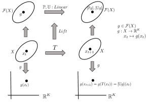
Figure 1: Koopman and Perron-Frobenius operators.

It can be shown that the P-F and the Koopman operators are dual to each other [4] in the sense that

$$\langle\mathbb{U}f,g\rangle=\langle f,\mathbb{P}g\rangle,$$

for $f\in L_{\infty}(Z)$ and $g\in L_{1}(Z)$.

The advantage of using the above operator theoretic approach is the fact that both the P-F operator and the Koopman operator are linear operators, even if the underlying system is non-linear. However, though the operators are linear, the trade-off is that these operators are typically infinite-dimensional. In particular, the P-F operator and the Koopman operator often lift a nonlinear dynamical system from a finite-dimensional space to generate an infinite-dimensional linear system in infinite dimensions.

Definition 3 (Koopman Eigenfunction (KEF))

An eigenfunction of the Koopman operator $\mathbb{U}$ is a non-zero observable $\phi_{\lambda}\in{\cal F}$ that satisfies

$${\mathbb{U}}\phi_{\lambda}=\lambda\phi_{\lambda},$$

where $\lambda\in\mathbb{C}$ is the Koopman eigenvalue (KE) corresponding to the KEF $\phi_{\lambda}$.

III Nonlinear Stabilization using Koopman Operator

In this section, we present the main theoretical results of the paper where we formulate an optimization problem for the design of state feedback stabilizing control law for a discrete-time control-affine system. For simplicity of presentation, we consider the case of a single input control system.

III-A Koopman Representation of the Nonlinear Control System

We consider a discrete-time control-affine system of the form

$$x_{t+1}=T(x_{t})+g(x_{t})u_{t}$$ (2)

where $x_{t}\in\mathbb{R}^{d}$, $u_{t}\in\mathbb{R}$ is the single input to the system and $T,g:\mathbb{R}^{d}\to\mathbb{R}^{d}$ are at least of class ${\cal C}^{2}$. Let $(\lambda_{i},\phi_{i})$, $i=1,2,\dots$ be the discrete eigenvalues and the corresponding eigenfunctions of the Koopman operator $\mathbb{U}$ for the unactuated system $x_{t+1}=T(x_{t})$.

Assumption 4

Let ${\cal F}^{n}=\textnormal{span}\{\phi_{i}\}_{i=1}^{n}$ be the span of a finite subset of the Koopman eigenfunctions such that $x\in{\cal F}^{n}$. Hence we have

$$x=\sum_{i=1}^{n}\phi_{i}(x){\bf v}_{i}^{x},$$ (3)

where ${\bf v}_{i}^{x}\in\mathbb{C}^{d}$ are the Koopman modes.

We follow the notation of [23] and order the Koopman eigenfunctions $\{\phi_{1},\cdots,\phi_{n}\}$ and the corresponding Koopman eigenvalues and Koopman modes such that the complex conjugate pairs are placed adjacent to each other. Let $\Phi(x)=\{\hat{\phi}_{1}(x),\cdots,\hat{\phi}_{n}(x)\}$, such that

1. $\hat{\phi}(x)=\phi_{i}(x)$ if the $i^{th}$ Koopman eigenfunction is real, and

2. $\hat{\phi}_{i}(x)=2\textnormal{Re}(\phi_{i})$ and $\hat{\phi}_{i+1}(x)=-2\textnormal{Im}(\phi_{i})$, if $i^{th}$ and $(i+1)^{th}$ Koopman eigenfunctions are complex conjugate pairs.

where $\textnormal{Re}(\cdot)$, $\textnormal{Im}(\cdot)$ denotes the real and imaginary part respectively. The Koopman mode decomposition (3) can now be written as

$$x=C^{x}\Phi(x),$$ (4)

where $C^{x}\in\mathbb{C}^{d\times n}$. Note that, since $x=C^{x}\Phi(x)$, the mapping $\Phi$ is injective onto its range and $\Phi(0)=0$. Moreover, the matrix $C^{x}$, which can be obtained from data as a solution to a least squares problem, is used to project the lifted trajectories $(z_{t}\in\mathbb{R}^{n})$ back to the state space $(x_{t}\in\mathbb{R}^{d})$.

We further assume the following.

Assumption 5

We assume that $\frac{\partial{\bf\Psi}}{\partial x}g$ lies in ${\cal F}^{n}$, so that there exists a constant matrix $B\in\mathbb{R}^{n\times n}$ such that $\frac{\partial{\bf\Psi}}{\partial x}g=B{\bf\Psi}$.

Remark 6

On the face of it, assumption 5 seems a bit restrictive and depends on the the functions $\hat{\phi}_{i}$ and $g$. In the cases where assumption 5 fails to hold, one can obtain the matrix $B$ as a solution of a least-squares problem where we have $\frac{\partial{\bf\Psi}}{\partial x}g=B\Phi+\varepsilon$, for $\varepsilon\in\mathbb{R}^{n}$, so that we minimize the norm of the error vector $\varepsilon$ to find the optimal $B$.

Lemma 7

Under assumption 5 and the set of observables (lifting functions) defined as $\Phi(x_{t})=z_{t}$, the Koopman representation of the control-affine system (2) is given by

$$z_{t+1}=\mathbb{U}z_{t}+u_{t}Bz_{t}.$$ (5)

Proof:

Let $z(t)=\Phi(x(t))$. Then we have,

$$z_{t+1} = \Phi(x_{t+1})=\Phi\Big{(}T(x_{t})+g(x_{t})u_{t}\Big{)}$$ (6)

$$\approx \Phi\big{(}T(x_{t})\Big{)}+\frac{\partial\Phi}{\partial x}g(x_{t})u_{t}+h.o.t.$$

$$= \mathbb{U}\Phi(x_{t})+\frac{\partial\Phi}{\partial x}g(x_{t})u_{t}$$

$$= \mathbb{U}z_{t}+\frac{\partial\Phi}{\partial x}g(x_{t})u_{t}$$

Now from assumption 5, $\frac{\partial\Phi}{\partial x}g(x_{t})=B\Phi(x_{t})=Bz_{t}$ and hence the Koopman representation (6) of the nonlinear system (2) becomes

$$z_{t+1}=\mathbb{U}z_{t}+u_{t}Bz_{t}.$$ (7)

Hence, for the control-affine system (2), the equivalent Koopman representation is a bilinear control system of the form (7). ∎

Note that under assumptions 4 and 5, the Koopman representation (7) is a finite-dimensional exact representation of the control-affine system (2). See [23] for the continuous-time counterpart of this.

III-B Controllability of the original and Koopman lifted system

The concepts of controllability and observability are fundamental notions in systems theory. But for general nonlinear systems, it is not always easy to determine whether it is controllable (observable). Moreover, in the case of nonlinear systems, there are multiple notions of controllability like accessibility, local controllability and global controllability [39]. For the completeness of the paper, we revisit some of the basic definitions related to controllability of nonlinear systems.

Definition 8 (Accessibility [39])

A nonlinear system is accessible from the state $x_{0}\in\mathbb{R}^{d}$ if the attainable set (both in forward and backward time) from $x_{0}$ has a non-empty interior.

Hence if a system is accessible from some $x_{0}$, it implies that starting from $x_{0}$ one can drive the system to some open subset of the configuration manifold. However, this does not imply controllability or even local controllability.

Definition 9 (Local Controllability [39])

A nonlinear system is locally controllable from $x_{0}\in\mathbb{R}^{d}$ if the reachable set from $x_{0}$ contains a neighbourhood of $x_{0}$.

In other words, local controllability implies that starting from $x_{0}$ the system can be driven to any point in the state space which is near $x_{0}$.

Theorem 10

The control-affine system (2) is locally controllable at $x_{0}$ if the Lie algebra of the vector field at $x_{0}$ span the tangent space at $x_{0}$, that is the rank of the Lie algebra generated by the vector field of (2) at $x_{0}$ is $d$, where $d$ is the dimension of the configuration manifold.

Proof:

See [39, 40]. ∎

In the case of linear systems, local controllability implies that the system is globally controllable, that is, if the trajectories from $x_{0}$ can be steered to all points of the state space that are in the local neighbourhood of $x_{0}$, it implies that the system can be driven to any point in the state space from any other point. However, for general nonlinear systems, this is not the case and the notion of global controllability for nonlinear systems is defined as follows.

Definition 11 (Global Controllability [39])

If a nonlinear system is locally controllable for all $x_{0}$ of the configuration manifold, then the system is globally controllable.

Note that the above definition does imply global controllability because a trajectory starting from any $x_{0}$ can be steered to any point in the state space by patching together trajectories obtained from local controllability and this patching can be achieved because the nonlinear system is locally controllable for all points in the state space.

We refer the reader to [39, 40] for further details.

III-B1 Controllability of general bilinear systems

Consider a general bilinear system of the form

$$z(t+1)=Az(t)+\sum_{i=1}^{l}u_{i}(t)B^{i}z(t)+B^{0}u_{0}(t),$$ (8)

where $z(t)\in\mathbb{R}^{n}$ are the states, $u_{i}(t)$ are scalar inputs with input matrices $B^{i}$. For the bilinear system (8), the drift vector field is $f_{d}=Az$ and define $\theta_{0}(z)=B^{0}$ and $\theta_{i}(z)=B^{i}z$ for $i=1,2,\dots,l$.

Theorem 12

The bilinear system (8) is globally controllable if the accessibility distribution

$${\cal Q}=\Big{[}B^{0},B^{1},\dots,B^{l},-AB^{0},\dots,(-1)^{n-1}A^{n-1}B^{0},$$

$$B^{1}B^{0},\dots,B^{l}B^{0},[B^{1},A]z,[B^{2},A]z,\dots,\big{[}[B^{l},A]A^{n-1}\big{]}z\Big{]}$$

has full rank, that is rank$({\cal Q})=n$ for all $z\in\mathbb{R}^{n}$.

Proof:

Local controllability of a general nonlinear system is characterized by the accessibility distribution ${\cal Q}=\textnormal{Lie}(\{X_{1},X_{2},\dots,X_{M}\})$, where $X_{i}$ are the vector fields for the nonlinear system. Hence, for analyzing the local controllability of the bilinear system (8), we need to compute the Lie brackets among the different vector fields. We have $f_{d}=Az$, $\theta_{0}(z)=B^{0}$ and $\theta_{i}(z)=B^{i}z$ for $i=1,2,\dots,l$. Hence,

$$[\theta_{0},\theta_{i}]=\frac{\partial\theta_{i}}{\partial z}\theta_{0}-\frac{\partial\theta_{0}}{\partial z}\theta_{i}=B^{i}B^{0}.$$ (9)

Hence the higher order Lie bracket

$$\big{[}\theta_{0},[\theta_{0},\theta_{i}]\big{]}=[\theta_{0},B^{i}B^{0}]=0,$$

that is,

$$\big{(}ad_{\theta_{0}}^{k},\theta_{i}\big{)}=0\textnormal{ for }k>1.$$ (10)

Next, we look at the Lie brackets between the drift vector field with $\theta_{0}$. In particular,

$$[f_{d},\theta_{0}]=\frac{\partial\theta_{0}}{\partial z}f_{d}-\frac{\partial f_{d}}{\partial z}\theta_{0}=-AB^{0}.$$ (11)

With this we have,

$$\big{(}ad_{f_{d}}^{k},\theta_{0}\big{)}=(-1)^{k}A^{k}B^{0}.$$ (12)

Similarly,

$$[f_{d},\theta_{i}]=\frac{\partial\theta_{i}}{\partial z}f_{d}-\frac{\partial f_{d}}{\partial z}\theta_{i}=B^{i}Az-AB^{i}z=[B^{i},A]z$$

and

$$\big{(}ad_{f_{d}}^{2},\theta_{i}\big{)}=\big{[}f_{d},[f_{d},\theta_{i}]\big{]}=\big{[}f_{d},[B^{i},A]z\big{]}=\big{[}[B^{i},A],A\big{]}z.$$

With this, one can compute $\big{(}ad_{f_{d}}^{k},\theta_{i}\big{)}$ as

$$\big{(}ad_{f_{d}}^{k},\theta_{i}\big{)}=\big{[}[B^{i},A],A^{k-1}\big{]}z.$$ (13)

Now, since $A\in\mathbb{R}^{n\times n}$, from Cayley-Hamilton theorem one needs to compute $\big{(}ad_{f_{d}}^{k},\theta_{i}\big{)}$ only upto for $k=n$ and then the accessibility matrix $\cal Q$ is

$${\cal Q} = \textnormal{Lie}(\{f_{d},\theta_{i},\theta_{0}\})$$ (14)

$$= \Big{[}B^{0},B^{1},\dots,B^{l},-AB^{0},\dots,(-1)^{n-1}A^{n-1}B^{0},$$

$$\quad B^{1}B^{0},\dots,B^{l}B^{0},[B^{1},A]z,[B^{2},A]z,\dots,$$

$$\qquad\big{[}[B^{l},A]A^{n-1}\big{]}z\Big{]}$$

Hence, the bilinear system (8) is locally controllable at $z_{0}\in\mathbb{R}^{d}$ if the rank of $\cal Q$ at $z_{0}$ is $d$ and from theorem 10 and definition 11 it is globally controllable if rank${\cal Q}=d$ for all $z\in\mathbb{R}^{d}$. ∎

III-B2 Controllability of the control-affine system and its Koopman representation

Given a control-affine system of the form (2) evolving in $\mathbb{R}^{d}$, lemma 7 gives the equivalent bilinear Koopman representation in $\mathbb{R}^{n}$. Again, theorem 12 gives sufficient conditions for global controllability of a bilinear system. With this, we have the following theorem relating controllability of the control-affine system (2) and its Koopman bilinear representation.

Theorem 13

Consider a control-affine system of the form

$$x_{t+1}=T(x_{t})+g(x_{t})u_{t},$$

$x_{t}\in\mathbb{R}^{d}$ and its bilinear Koopman representation of the form

$$z_{t+1}=\mathbb{U}z_{t}+u_{t}Bz_{t},$$

with $z_{t}\in\mathbb{R}^{d}$, such that $\Phi:\mathbb{R}^{d}\rightarrow\mathbb{R}^{n}$ are the set of observables. Then if the Koopman bilinear form is controllable, then the nonlinear control-affine system is also controllable.

Proof:

We prove this by contrapositive arguments. Suppose that for the nonlinear control-affine system $x_{t+1}=T(x_{t})+g(x_{t})u_{t}$, there exists $x_{0}$ and $x_{T}$ such that there does not exist any control $u_{t}$ which can drive the system trajectory from $x_{0}$ to $x_{T}$ in time $T$. Let ${\cal T}(x_{0},u)$ be the set of all control trajectories that start from $x_{0}$. Hence

$${\cal T}(x_{0},u)\cap x_{T}=\{\varphi\},$$

where $\{\varphi\}$ denotes the empty set. Let $\Phi\big{(}{\cal T}(x_{0},u)\big{)}$ and $\Phi(x_{T})$ be the images of ${\cal T}(x_{0})$ and $x_{T}$ under the observables $\Phi$. Since the mapping $\Phi$ is injective, in the lifted space we again have

$$\Phi\big{(}{\cal T}(x_{0},u)\big{)}\cap\Phi(x_{T})=\{\varphi\}.$$

Hence, if the control-affine system is uncontrollable, then the lifted Koopman bilinear system is also uncontrollable. In other words, if the lifted Koopman bilinear system is controllable then so is the original control-affine nonlinear system. ∎

III-C Control Lyapunov Function

Now that we have related the controllability properties of the control-affine system with those of the lifted Koopman bilinear system, we now address the problem of stabilization of the nonlinear control system.

The control objective is to design a state feedback control law $u_{t}=k(x_{t})$, with $k:\mathbb{R}^{d}\to\mathbb{R}$, such that the origin $x=0$ is asymptotically stable within some domain $\Omega\in\mathbb{R}^{d}$ for the closed loop system

$$x_{t+1}=T(x_{t})+g(x_{t})k(x_{t}).$$ (15)

Definition 14 (Control Lyapunov Function)

Let $V(x_{t})$ be a radially unbounded, positive definite function with $V(x_{t})>0$, $\forall x_{t}\neq 0$ and $V(0)=0$. If for any $x_{t}\in\mathbb{R}^{d}$, there exist real values $u_{t}$ such that

$$\Delta V(x_{t},u_{t})<0,$$

where $\Delta V(x_{t},u_{t})=V(x_{t+1})-V(x_{t})$, then $V(\cdot)$ is called the discrete-time control Lyapunov function for the system (2).

In the subsequent subsection, we will use the concept of control Lyapunov function to prove the stability of the origin of the closed-loop system.

III-D Stabilization of Control-affine Systems

Given a nonlinear control-affine system (2), we seek a stabilizing control law of the form $u=k(z)$ which stabilizes the origin of the system (2) and we do so by considering the bilinear Koopman representation of the control-affine system. In particular, we seek a state feedback control law $u_{t}=k(z_{t})$ in the lifted space $\mathbb{R}^{n}$ which quadratically stabilizes the system (7) inside the ellipsoid

$$\mathscr{E}=\{z\in\mathbb{R}^{n}|z^{\top}Q^{-1}z\leq 1\},\quad Q\succ 0.$$

The design of stabilizing control law for general bilinear systems has been addressed in the literature and interested readers are referred to [41, 42, 43, 44]. The theorem here is stated and proved to suit the framework of the problem at hand.

To prove the stabilizability theorem, we need the following lemma [45]:

Lemma 15

Let $G=G^{\top}\in\mathbb{R}^{n\times n}$, $M\in\mathbb{R}^{n\times q}$, $N\in\mathbb{R}^{n}$ and $0\prec P=P^{\top}\in\mathbb{R}^{q\times q}$. The matrix inequality

$$G+M\delta N^{\top}+N\delta^{\top}M^{\top}\prec 0$$

holds for all $\delta\in\mathbb{R}^{q}$, $\delta^{\top}P\delta\leq 1$ if and only if there exists a real number $\varepsilon$ such that

$$\begin{pmatrix}G&M&N\\ M^{\top}&-\varepsilon P&0\\ N^{\top}&0&-\frac{1}{\varepsilon}I\end{pmatrix}\prec 0.$$

where 0 and $I$ denotes matrix with all zeros and identity matrix of appropriate dimensions respectively.

With this, we have the following theorem.

Theorem 16

Let a positive symmetric matrix $Q=Q^{\top}>0$ and a vector $y$ be such that the matrix inequality

$$\begin{pmatrix}-Q&0&y&Q\mathbb{U}^{\top}\\ 0&-\varepsilon Q&0&QB^{\top}\\ y^{\top}&0&-\frac{1}{\varepsilon}I&0\\ \mathbb{U}Q&BQ&0&-Q\end{pmatrix}\prec 0$$ (16)

is satisfied for some $\varepsilon\in\mathbb{R}$. Then the linear feedback with controller gain $k=Q^{-1}y$ stabilizes the bilinear system

$$z_{t+1}=\mathbb{U}z_{t}+u_{t}Bz_{t}$$

inside the ellipsoid

$$\mathscr{E}=\{z\in\mathbb{R}^{n}:z^{\top}Q^{-1}z\leq 1\},$$

and the quadratic form $V(z)=z^{\top}Q^{-1}z$ is control Lyapunov function for the bilinear system (7).

Proof:

Consider the quadratic Lyapunov function $V(z)=z^{\top}Pz$ for $P=P^{\top}>0$. Then

$$\Delta V = V(z_{t+1})-V(z_{t})$$ (17)

$$= (\mathbb{U}z_{t}+u_{t}Bz_{t})^{\top}P(\mathbb{U}z_{t}+u_{t}Bz_{t})-z_{t}^{\top}Pz_{t}$$

$$= z_{t}^{\top}(\mathbb{U}^{\top}P\mathbb{U}-P)z_{t}+uz_{t}^{\top}(\mathbb{U}^{\top}PB+B^{\top}P\mathbb{U})z_{t}$$

$$\quad+u^{2}z_{t}^{\top}B^{\top}PBz_{t}$$

For the system (7) to be stable, $\Delta V<0$ for $z\neq 0$. We seek a state feedback control law $u_{t}=k(z_{t})$ that stabilizes the origin. Hence, for stabilizability, rewriting (17) in matrix form, we have

$$\begin{pmatrix}\mathbb{U}^{\top}P\mathbb{U}-P&k(z)B^{\top}P\\ +k(z)\mathbb{U}^{\top}PB+k(z)B^{\top}P\mathbb{U}\\ PBk(z)&-P\end{pmatrix}\prec 0.$$ (18)

Under the assumption that we use linear feedback control $u=k^{\top}z$, we have

$$\begin{pmatrix}\mathbb{U}^{\top}P\mathbb{U}-P&0\\ 0&-P\end{pmatrix}+\begin{pmatrix}\mathbb{U}^{\top}PB\\ PB\end{pmatrix}z\begin{pmatrix}k^{\top}&0\end{pmatrix}+$$

$$\begin{pmatrix}k\\ 0\end{pmatrix}z^{\top}\begin{pmatrix}B^{\top}P\mathbb{U}&B^{\top}P\end{pmatrix}\prec 0.$$ (19)

The goal is to make the above matrix inequality (III-D) hold for all $z$ from the ellipsoid

$$\mathscr{E}=\{z\in\mathbb{R}^{n}:z^{\top}Pz\leq 1\}.$$

Using lemma 15, equation (III-D) can be equivalently written as

$$\begin{pmatrix}\mathbb{U}^{\top}P\mathbb{U}-P&0&\mathbb{U}^{\top}PB&k\\ 0&-P&PB&0\\ B^{\top}P\mathbb{U}&B^{\top}P&-\varepsilon P&0\\ k^{\top}&0&0&-\frac{1}{\varepsilon}I\end{pmatrix}\prec 0.$$ (20)

The feasibility of (20) implies stability and thus the feedback control law $u=k^{\top}z$ stabilizes the bilinear control system

$$z_{t+1}=\mathbb{U}z_{t}+u_{t}Bz_{t}.$$

Using Schur’s Lemma, from (20) we have

$$\begin{pmatrix}\mathbb{U}^{\top}P\mathbb{U}-P&\mathbb{U}^{\top}PB&k\\ B^{\top}P\mathbb{U}&B^{\top}P-\varepsilon P&0\\ k^{\top}&0&-\frac{1}{\varepsilon}I\end{pmatrix}\prec 0$$ (21)

which can be further written as

$$\begin{pmatrix}-P&0&k\\ 0&-\varepsilon P&0\\ k^{\top}&0&-\frac{1}{\varepsilon}I\end{pmatrix}+\begin{pmatrix}\mathbb{U}^{\top}\\ B^{\top}\\ 0\end{pmatrix}P\begin{pmatrix}\mathbb{U}&B&0\end{pmatrix}\prec 0.$$ (22)

Applying Schur’s Lemma to (22), we have

$$\begin{pmatrix}-P&0&k&\mathbb{U}^{\top}\\ 0&-\varepsilon P&0&B^{\top}\\ k^{\top}&0&-\frac{1}{\varepsilon}I&0\\ \mathbb{U}&B&0&-P^{-1}\end{pmatrix}\prec 0.$$ (23)

Let $Q=P^{-1}$ and pre- and post-multiplying (23) by $\textnormal{diag}(Q,Q,I,I)$, we have

$$\begin{pmatrix}-Q&0&Qk&Q\mathbb{U}^{\top}\\ 0&-\varepsilon Q&0&QB^{\top}\\ k^{\top}Q&0&-\frac{1}{\varepsilon}I&0\\ \mathbb{U}Q&BQ&0&-Q\end{pmatrix}\prec 0.$$ (24)

Setting $y=Qk\in\mathbb{R}^{n}$, we have the proof. ∎

The above theorem proves the existence of a state feedback stabilizing control law that stabilizes the origin of a bilinear control system. However, we can do more. In particular, we can strive to maximize the stabilizability ellipsoid. One way to do it is to maximize the volume of the stabilizability ellipsoid. This can be achieved in the following way:

Corollary 17

Consider the optimization problem:

$$\begin{aligned} &\qquad\quad\max\log\det Q\\ \textnormal{subject to }&\begin{pmatrix}-Q&0&y&Q\mathbb{U}^{\top}\\ 0&-\varepsilon Q&0&QB^{\top}\\ y^{\top}&0&-\frac{1}{\varepsilon}I&0\\ \mathbb{U}Q&BQ&0&-Q\end{pmatrix}\prec 0\end{aligned}$$ (25)

with respect to the optimization variables $Q=Q^{\top}\in\mathbb{R}^{n\times n}$ and $y\in\mathbb{R}^{n}$. Then the ellipsoid

$$\hat{\mathscr{E}}=\{z\in\mathbb{R}^{n}:z^{\top}Q^{-1}z\leq 1\}$$

is the stabilizability ellipsoid of the system (7) with the feedback control law given by $u=\hat{k}^{\top}z$, where $\hat{k}=\hat{Q}^{-1}\hat{y}$.

Though the optimization problem (25) of corollary (17) maximizes the stabilizability ellipsoid, the objective function is optimized under a strict constraint. To make the problem well-posed, we make the strict inequality a non-strict inequality as follows:

$$\begin{pmatrix}-\theta Q&0&y&Q\mathbb{U}^{\top}\\ 0&-\varepsilon Q&0&QB^{\top}\\ y^{\top}&0&-\frac{1}{\varepsilon}I&0\\ \mathbb{U}Q&BQ&0&-Q\end{pmatrix}\preceq 0$$ (26)

where $0<\theta<1$. Hence, the feedback control law which maximizes the stabilizability ellipsoid is obtained as the solution of the following optimization problem:

$$\begin{aligned} &\qquad\quad\max\log\det Q\\ \textnormal{subject to }&\begin{pmatrix}-\theta Q&0&y&Q\mathbb{U}^{\top}\\ 0&-\varepsilon Q&0&QB^{\top}\\ y^{\top}&0&-\frac{1}{\varepsilon}I&0\\ \mathbb{U}Q&BQ&0&-Q\end{pmatrix}\preceq 0.\end{aligned}$$ (27)

Theorem 16 provides a state feedback control law that stabilizes the origin of a bilinear control system , which in our case is the lifted Koopman system. Now, the mapping $\Phi$ is such that $\Phi(0)=0$. Hence the stabilized trajectories of the lifted bilinear Koopman system, which converge to the origin of the lifted space $\mathbb{R}^{n}$, when projected back to the original state space $\mathbb{R}^{d}$, they too converge to the origin of the state space. Thus the state feedback control law stabilizes the origin of the nonlinear control-affine system.

IV Extended Dynamic Mode Decomposition (EDMD)

Typically, the Koopman operator $(\mathbb{U})$ for a dynamical system is infinite-dimensional and hence for data-driven computations, a finite-dimensional approximation of the Koopman operator is computed from the time-series data. Moreover, satisfying assumptions 4 and 5 is difficult. In this section, we briefly describe the procedure for computing the approximate system matrices of the lifted bilinear system from time-series data.

Consider snapshots of time-series data

$$X=[x_{1},x_{2},\cdots,x_{M}],\quad Y=[y_{1},y_{2},\cdots,y_{M}],$$

obtained from simulating a discrete time dynamical system $y_{i}=T(x_{i})$ or from an experiment, where $x_{i}$ and $y_{i}$ are consecutive data points. Let $x_{i},y_{i}\in\mathbb{R}^{d}$. Let $\Phi=\{\phi_{1},\phi_{2},\ldots,\phi_{n}\}$ be the set of dictionary functions or observables, where $\phi_{i}:\mathbb{R}^{d}\to\mathbb{C}$. Let ${\cal G}_{\Phi}$ denote the span of ${\Phi}$ such that ${\cal G}_{\Phi}\subset L_{2}(X,{\cal B},\mu)$. One important observation is the fact that for a good approximation of the Koopman operator, the set of dictionary functions should be able to approximate the leading eigenfunctions of the Koopman operator.

With this, if $\bf K$ is the finite dimensional approximation of the Koopman operator, then the matrix $\bf K$ can be obtained as a solution to the following least square problem [7].

$$\min\limits_{\bf K}\parallel{\bf G}{\bf K}-{\bf A}\parallel_{F}$$ (28)

$$\begin{aligned} &{\bf G}=\frac{1}{M}\sum_{m=1}^{M}{\Phi}({x}_{m})^{\top}{\Phi}({x}_{m})\\ &{\bf A}=\frac{1}{M}\sum_{m=1}^{M}{\Phi}({x}_{m})^{\top}{\Phi}({y}_{m}),\end{aligned}$$ (29)

with ${\bf K},{\bf G},{\bf A}\in\mathbb{C}^{n\times n}$. The optimization problem (28) can be solved explicitly to obtain following solution for the matrix $\bf K$, i.e.,

$${\bf K}_{EDMD}={\bf G}^{\dagger}{\bf A},$$ (30)

where ${\bf G}^{\dagger}$ is the Moore-Penrose inverse of matrix $\bf G$. Dynamic Mode Decomposition (DMD) is a special case of EDMD algorithm with ${\Phi}(x)=x$.

Now, within the setting of this paper, since the Koopman representation of the nonlinear system (2) is a bilinear system of the form (7), the finite-dimensional representation of the control-affine system (2) will take the form

$$z_{t+1}=Az_{t}+u_{t}Bz_{t}.$$ (31)

It is assumed that the leading Koopman eigenfunctions are contained inside ${\cal G}_{\Phi}$, and the eigenvalues of ${\bf K}_{EDMD}$ are approximations of the Koopman eigenvalues. Let the right eigenvectors of Koopman ${\bf K}_{EDMD}$ be denoted by $v_{j}$, $j=1,\ldots,n$. Then the Koopman eigenfunctions are approximated using the right eigenvectors and the dictionary as

$$h_{j} ={\Phi}^{\top}v_{j},\quad j=1,2,\dots,n,$$ (32)

where $h_{j}$ is the approximation of the eigenfunction of Koopman operator corresponding to the $j^{th}$ eigenvalue. For the bilinear system (31), the system matrix $A$ on the lifted space is expressed as a block diagonal matrix of Koopman eigenvalues $\lambda_{1},\lambda_{2},\dots,\lambda_{n}$ where

1. ${A}_{(i,i)}=\lambda_{i}$ if $h_{i}$ is real, and

2. if $h_{i}$ and $h_{i+1}$ are complex conjugate pairs, then $\begin{bmatrix}{A}_{i,i}&{A}_{i,i+1}\\ {A}_{i+1,i}&{A}_{i+1,i+1}\end{bmatrix}$ = $|\lambda_{i}|\begin{bmatrix}\cos(\angle\lambda_{i})&\sin(\angle\lambda_{i})\\ -\sin(\angle\lambda_{i})&\cos(\angle\lambda_{i})\end{bmatrix}$

From (32), while the Koopman eigenfunctions are real-valued, we have,

$$H(x)=V^{\top}{\bf\Psi}(x),$$

where

$$V=\begin{bmatrix}v_{1}&v_{2}&\ldots&v_{n}\end{bmatrix}$$

$$H(x)=\begin{bmatrix}h_{1}(x)&h_{2}(x)&\dots&h_{n}(x)\end{bmatrix}.$$

We now approximate the matrix $B\in\mathbb{R}^{n\times n}$ as

$$\frac{\partial H}{\partial x}g(x) =V^{\top}\frac{\partial{\Phi}}{\partial x}g(x)$$

$$=BH(x)=BV^{\top}{\Phi}(x)=\tilde{B}{\Phi}(x).$$

Under the assumption that the observable functions ${\Phi}$ is a collection of monomial functions, the terms $\frac{\partial{\Phi}}{\partial x}$ lies in the span of ${\Phi}(x)$. Furthermore, the eigenvector matrix, $V$ is invertible and hence the $\tilde{B}$ can be found explicitly. Finally, the matrix $B$ can be computed such that $B=\tilde{B}(V^{\top})^{-1}$.

V Simulation Results

This section discusses two nonlinear dynamical systems where we stabilize the origin using our proposed approach. In particular, we stabilize the origin for the Van der Pol oscillator and the Henon map.

V-A Van der Pol Oscillator

The Van der Pol oscillator is a non-conservative dynamical system with nonlinear damping whose equations of motion are given by

$$\begin{aligned} &\dot{x}=y\\ &\dot{y}=\mu(1-x^{2})y-x.\end{aligned}$$ (33)

The constant $\mu\geq 0$ controls the damping and when $\mu=0$, one recovers the simple harmonic oscillator, which is a conservative system. For $\mu>0$, the system exhibits stable limit cycle oscillations, with the origin being an unstable equilibrium point. The invariant measure for the Van der Pol oscillator is shown in Fig. 2.

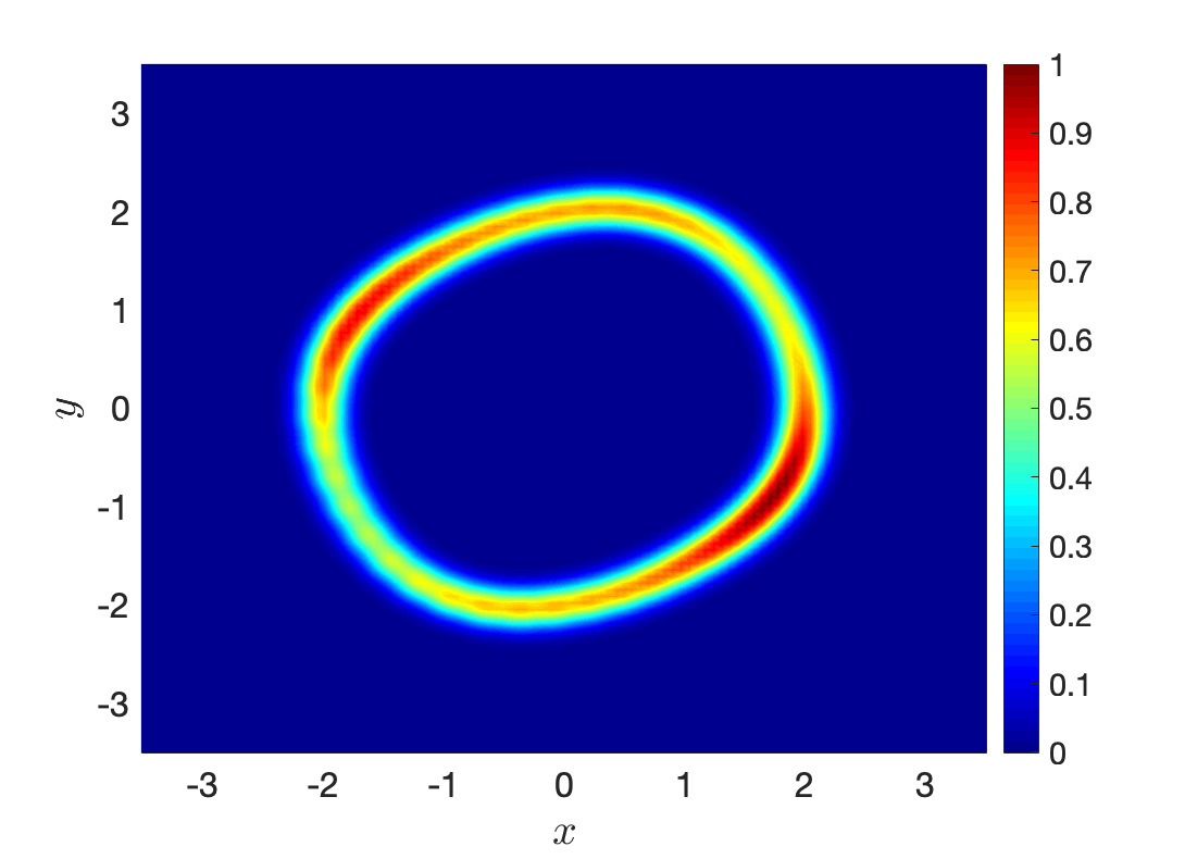
Figure 2: Invariant measure of the unforced Van der Pol oscillator.

The goal is to stabilize the origin by designing a state feedback law. To this end, we assume the following controlled Van der Pol oscillator:

$$\begin{aligned} &\dot{x}=y\\ &\dot{y}=\mu(1-x^{2})y-x+u,\end{aligned}$$ (34)

where $u$ is the scalar control input. Comparing (34) with (2), we have $g(x,y)=[0\quad 1]^{\top}$.

For simulation purposes, the constant $\mu$ was set to one and data was collected for 10 seconds with discretization step $\delta t=.01$ seconds. Furthermore, as dictionary functions, we used monomials up to order 5. Hence cardinality of the dictionary function set $(\Phi)$ is 21, so that the Koopman operator ${\bf K}\in\mathbb{R}^{21\times 21}$. Once the Koopman operator for the open-loop system is computed, the optimization problem (27) computes the optimal stabilizability ellipsoid $(\hat{Q})$ and the vector $y$. For simulation purposes, the parameter $\theta$ and $\varepsilon$ were set to 0.001 and 0.01 respectively. With this, the feedback control law gain $(k)$ in the lifted space is computed as $k=\hat{Q}^{-1}y$ and the feedback control law in the lifted space is given by $k^{\top}z$, where $z={\Phi}(x,y)$.

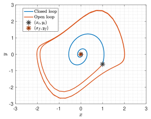
Figure 3: Open loop and closed loop trajectory for the Van der Pol oscillator. Without any control the open loop trajectory settles on the stable limit cycle, while with the state feedback control, the closed loop trajectory goes to the origin.

Fig. 3 shows the open and closed-loop trajectories for the Van der Pol oscillator starting from a random initial condition. We observe that the trajectory settles to the stable limit cycle attractor without the control input, whereas with the control law, the closed-loop trajectory is stabilized to the origin.

V-B Henon Map

The Henon map is a discrete-time dynamical system which exhibits chaotic behaviour. The equations of motion are

$$\begin{aligned} &x_{n+1}=1-ax_{n}^{2}+y_{n}\\ &y_{n+1}=bx_{n}.\end{aligned}$$ (35)

For the classical Henon map, with constants $a=1.4$ and $b=0.3$, the Henon map has a chaotic attractor, as shown by the invariant measure in Fig. 4.

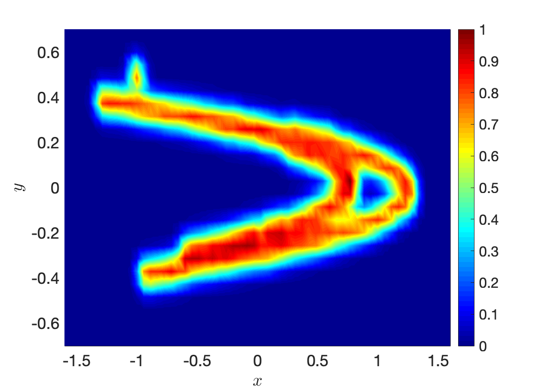
Figure 4: Invariant measure of the unforced Henon map.

We assume that the control map $g(x,y)=[0\quad 1]^{\top}$ so that the controlled Henon map is given by

$$\begin{aligned} &x_{n+1}=1-ax_{n}^{2}+y_{n}\\ &y_{n+1}=bx_{n}+u.\end{aligned}$$ (36)

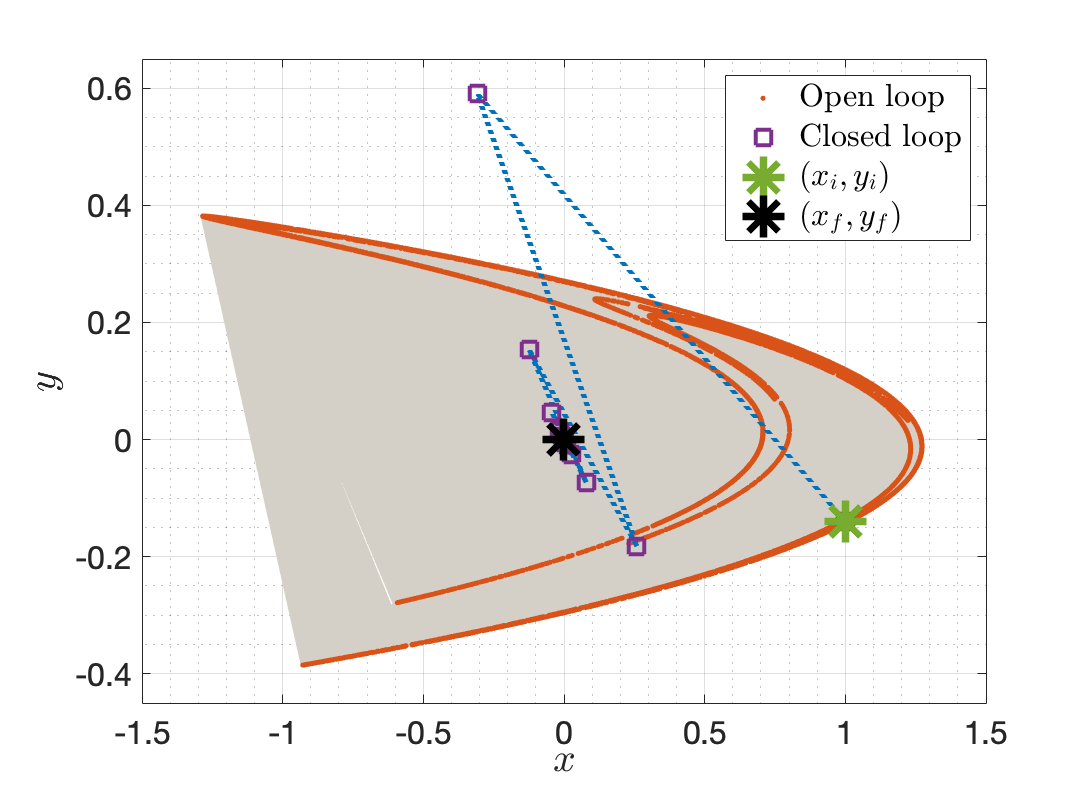
Figure 5: Open loop and closed loop trajectory for the Henon map. Without any control the open loop trajectory settles on the chaotic attractor, while with the state feedback control, the closed loop trajectory goes to the origin.

The data for the uncontrolled Henon map (35) was generated for 10000-time steps and the Koopman operator was computed using monomials up to degree 2. Hence the cardinality of the dictionary function set $\Phi$ is five so that the Koopman operator ${\bf K}\in\mathbb{R}^{5\times 5}$. The optimization problem (27) yields the state feedback control law. Subsequently, in Fig. 5, we show both the open and closed-loop trajectory, starting from a random initial condition. It can be seen that the trajectory for the uncontrolled system settles on the chaotic attractor. In contrast, the trajectory evolves to the origin of the controlled system, thus stabilizing the origin. However, one may note that the closed-loop trajectory is non-smooth, unlike the Van der Pol oscillator, and this is due to the nature of the trajectories of the uncontrolled Henon map.

VI Conclusions

This paper develops a data-driven method for designing a stabilizing control law for general discrete-time control-affine systems. In particular, we use the Koopman operator framework to lift the dynamical system to a higher dimensional space where the evolution is given by a bilinear system. Before the design of the state feedback control law, we analyzed the controllability of the lifted bilinear system and related it to the controllability of the original nonlinear control-affine system. With this, we designed a state feedback stabilizing control law in the higher dimensional space for the bilinear system and proved that this state-feedback law quadratically stabilizes the origin of the bilinear control system in the higher dimensional space. Furthermore, we proposed an optimization problem that maximizes the stabilizability ellipsoid. The proposed approach is demonstrated to stabilize the origin of the Van der Pol oscillator (a nonlinear system with a stable limit cycle) and the Henon map (a chaotic system) from time-series data.

References

- [1] D. Henrion and A. Garulli, Positive polynomials in control. Springer Science & Business Media, 2005, vol. 312.
- [2] P. A. Parrilo, “Structured semidefinite programs and semialgebraic geometry methods in robustness and optimization,” Ph.D. dissertation, California Institute of Technology, 2000.
- [3] E. D. Sontag, “Feedback stabilization of nonlinear systems,” Robust control of linear systems and nonlinear control, pp. 61–81, 1990.
- [4] A. Lasota and M. C. Mackey, Chaos, Fractals, and Noise: Stochastic Aspects of Dynamics. New York: Springer-Verlag, 1994.
- [5] I. Mezic and A. Banaszuk, “Comparison of systems with complex behavior: spectral methods,” in Proceedings of the 39th IEEE Conference on Decision and Control (Cat. No.00CH37187), vol. 2, 2000, pp. 1224–1231 vol.2.
- [6] U. Vaidya and P. G. Mehta, “Lyapunov measure for almost everywhere stability,” IEEE Transactions on Automatic Control, vol. 53, no. 1, pp. 307–323, 2008.
- [7] M. O. Williams, I. G. Kevrekidis, and C. W. Rowley, “A Data–Driven Approximation of the Koopman Operator: Extending Dynamic Mode Decomposition,” Journal of Nonlinear Science, vol. 25, no. 6, pp. 1307–1346, 2015.
- [8] S. Sinha, U. Vaidya, and E. Yeung, “On computation of Koopman operator from sparse data,” in 2019 American Control Conference (ACC). IEEE, 2019, pp. 5519–5524.
- [9] M. Budisic, R. Mohr, and I. Mezic, “Applied Koopmanism,” Chaos, vol. 22, pp. 047 510–32, 2012.
- [10] S. Sinha, S. P. Nandanoori, and E. Yeung, “Koopman operator methods for global phase space exploration of equivariant dynamical systems,” IFAC-PapersOnLine, vol. 53, no. 2, pp. 1150–1155, 2020.
- [11] S. P. Nandanoori, S. Sinha, and E. Yeung, “Data-driven operator theoretic methods for global phase space learning,” in 2020 American Control Conference (ACC). IEEE, 2020, pp. 4551–4557.
- [12] ——, “Data-driven operator theoretic methods for phase space learning and analysis,” arXiv preprint arXiv:2106.15678, 2021.
- [13] S. Sinha, U. Vaidya, and E. Yeung, “On Few Shot Learning of Dynamical Systems: A Koopman Operator Theoretic Approach,” arXiv preprint arXiv:2103.04221, 2021.
- [14] S. Sinha and U. Vaidya, “Causality preserving information transfer measure for control dynamical system,” in 2016 IEEE 55th Conference on Decision and Control (CDC). IEEE, 2016, pp. 7329–7334.
- [15] ——, “On information transfer in discrete dynamical systems,” in 2017 Indian Control Conference (ICC). IEEE, 2017, pp. 303–308.
- [16] S. Sinha, P. Sharma, U. Vaidya, and V. Ajjarapu, “Identifying causal interaction in power system: Information-based approach,” in 2017 IEEE 56th Annual Conference on Decision and Control (CDC). IEEE, 2017, pp. 2041–2046.
- [17] ——, “On information transfer-based characterization of power system stability,” IEEE Transactions on Power Systems, vol. 34, no. 5, pp. 3804–3812, 2019.
- [18] S. Sinha, B. Huang, and U. Vaidya, “On robust computation of Koopman operator and prediction in random dynamical systems,” Journal of Nonlinear Science, pp. 1–34, 2019.
- [19] N. Črnjarić-Žic, S. Maćešić, and I. Mezić, “Koopman operator spectrum for random dynamical system,” arXiv preprint arXiv:1711.03146, 2017.
- [20] B. Lusch, J. N. Kutz, and S. L. Brunton, “Deep learning for universal linear embeddings of nonlinear dynamics,” Nature communications, vol. 9, no. 1, pp. 1–10, 2018.
- [21] E. Yeung, S. Kundu, and N. Hodas, “Learning deep neural network representations for Koopman operators of nonlinear dynamical systems,” in 2019 American Control Conference (ACC). IEEE, 2019, pp. 4832–4839.
- [22] S. P. Nandanoori, S. Guan, S. Kundu, S. Pal, K. Agarwal, Y. Wu, and S. Choudhury, “Graph neural network and koopman models for learning networked dynamics: A comparative study on power grid transients prediction,” IEEE Access, pp. 1–1, 2022.
- [23] A. Surana, “Koopman operator based observer synthesis for control-affine nonlinear systems,” in 2016 IEEE 55th Conference on Decision and Control (CDC). IEEE, 2016, pp. 6492–6499.
- [24] S. Sinha, U. Vaidya, and R. Rajaram, “Operator theoretic framework for optimal placement of sensors and actuators for control of nonequilibrium dynamics,” Journal of Mathematical Analysis and Applications, vol. 440, no. 2, pp. 750–772, 2016.
- [25] S. Sinha, U. Vaidya, and E. Yeung, “On information transfer in dynamical systems with applications in control of non-equilibrium dynamics,” in 2019 Sixth Indian Control Conference (ICC). IEEE, 2019, pp. 326–331.
- [26] S. Sinha and U. Vaidya, “Data-driven approach for inferencing causality and network topology,” in 2018 Annual American Control Conference (ACC). IEEE, 2018, pp. 436–441.
- [27] ——, “On data-driven computation of information transfer for causal inference in discrete-time dynamical systems,” Journal of Nonlinear Science, vol. 30, no. 4, pp. 1651–1676, 2020.
- [28] Y. Susuki and I. Mezić, “Nonlinear Koopman modes and power system stability assessment without models,” IEEE Transactions on Power Systems, vol. 29, no. 2, pp. 899–907, 2013.
- [29] S. Sinha, S. P. Nandanoori, and E. Yeung, “Computationally Efficient Learning of Large Scale Dynamical Systems: A Koopman Theoretic Approach,” in 2020 IEEE International Conference on Communications, Control, and Computing Technologies for Smart Grids (SmartGridComm). IEEE, 2020, pp. 1–6.
- [30] ——, “Data driven online learning of power system dynamics,” in 2020 IEEE Power & Energy Society General Meeting (PESGM). IEEE, 2020, pp. 1–5.
- [31] S. P. Nandanoori, S. Kundu, S. Pal, K. Agarwal, and S. Choudhury, “Model-agnostic algorithm for real-time attack identification in power grid using Koopman modes,” in 2020 IEEE International Conference on Communications, Control, and Computing Technologies for Smart Grids (SmartGridComm). IEEE, 2020, pp. 1–6.
- [32] A. Hasnain, S. Sinha, Y. Dorfan, A. E. Borujeni, Y. Park, P. Maschhoff, U. Saxena, J. Urrutia, N. Gaffney, D. Becker et al., “A data-driven method for quantifying the impact of a genetic circuit on its host,” in 2019 IEEE Biomedical Circuits and Systems Conference (BioCAS). IEEE, 2019, pp. 1–4.
- [33] E. Kaiser, J. N. Kutz, and S. L. Brunton, “Data-driven discovery of Koopman eigenfunctions for control,” arXiv preprint arXiv:1707.01146, 2017.
- [34] J. L. Proctor, S. L. Brunton, and J. N. Kutz, “Generalizing Koopman theory to allow for inputs and control,” SIAM Journal on Applied Dynamical Systems, vol. 17, no. 1, pp. 909–930, 2018.
- [35] M. Korda and I. Mezić, “Linear predictors for nonlinear dynamical systems: Koopman operator meets model predictive control,” arXiv preprint arXiv:1611.03537, 2016.
- [36] B. Huang, X. Ma, and U. Vaidya, “Feedback stabilization using Koopman operator,” in 2018 IEEE Conference on Decision and Control (CDC). IEEE, 2018, pp. 6434–6439.
- [37] X. Ma, B. Huang, and U. Vaidya, “Optimal quadratic regulation of nonlinear system using Koopman operator,” in 2019 American Control Conference (ACC). IEEE, 2019, pp. 4911–4916.
- [38] B. Huang and U. Vaidya, “A Convex Approach to Data-driven Optimal Control via Perron-Frobenius and Koopman Operators,” arXiv preprint arXiv:2010.01742, 2020.
- [39] F. Bullo and A. D. Lewis, Geometric control of mechanical systems: modeling, analysis, and design for simple mechanical control systems. Springer, 2019, vol. 49.
- [40] B. Jakubczyk and E. D. Sontag, “Controllability of nonlinear discrete-time systems: A lie-algebraic approach,” SIAM Journal on Control and Optimization, vol. 28, no. 1, pp. 1–33, 1990.
- [41] Z. Artstein, “Stabilization with relaxed controls,” Nonlinear Analysis: Theory, Methods & Applications, vol. 7, no. 11, pp. 1163–1173, 1983.
- [42] A. Astolfi, “Feedback stabilization of nonlinear systems,” Encyclopedia of Systems and Control, p. 437–447, 2015.
- [43] C. Xiushan, W. Xiaodong, and L. Ganyun, “Stabilization of discrete nonlinear systems based on control Lyapunov functions,” Journal of Systems Engineering and Electronics, vol. 19, no. 1, pp. 131–133, 2008.
- [44] M. V. Khlebnikov, “Quadratic stabilization of bilinear control systems,” Automation and Remote Control, vol. 77, no. 6, pp. 980–991, 2016.
- [45] I. R. Petersen, “A stabilization algorithm for a class of uncertain linear systems,” Systems & Control Letters, vol. 8, no. 4, pp. 351–357, 1987.