Flow rate–pressure drop relation for deformable channels
via fluidic and elastic reciprocal theorems

Abstract

Viscous flows through configurations manufactured or naturally assembled from soft materials apply both pressure and shear stress at the solid–liquid interface, leading to deformation of the fluidic conduit’s cross-section, which in turn affects the flow rate–pressure drop relation. Conventionally, calculating this flow rate–pressure drop relation requires solving the complete elastohydrodynamic problem, which couples the fluid flow and elastic deformation. In this Letter, we use the reciprocal theorems for Stokes flow and linear elasticity to derive a closed-form expression for the flow rate–pressure drop relation in deformable microchannels, bypassing the detailed calculation of the solution to the fluid-structure-interaction problem. For small deformations (under a domain perturbation scheme), our theory provides the leading-order effect of the interplay between the fluid stresses and the compliance of the channel on the flow rate–pressure drop relation. Our approach uses solely the fluid flow solution and the elastic deformation due to the corresponding fluid stress distribution in an undeformed channel, eliminating the need to solve the coupled elastohydrodynamic problem. Unlike previous theoretical studies that neglected the presence of lateral sidewalls (and considered shallow geometries of effectively infinite width), our approach allows us to determine the influence of confining sidewalls on the flow rate–pressure drop relation. In particular, for the flow-rate-controlled situation and the Kirchhoff–Love plate-bending theory for the elastic deformation, we show a trade-off between the effect of compliance of the deforming top wall and the drag due to sidewalls on the pressure drop. While compliance decreases the pressure drop, the drag due to sidewalls increases it. Our theoretical framework may provide insight into existing experimental data and pave the way for the design of novel optimized soft microfluidic configurations of different cross-sectional shapes.

I Introduction

Pressure-driven viscous flows through conduits manufactured from soft materials apply both pressure and shear stress at the solid–liquid interface, leading to deformation of the cross-section, which in turn affects the relationship between the flow rate $q$ and the pressure drop $\Delta p$ Gervais et al. (2006); Seker et al. (2009); Christov (2022). Understanding this $q-\Delta p$ relation is important for various microfluidic, lab-on-a-chip, biomedical, and soft robotics applications, such as pressure-actuated valves Thorsen et al. (2002), passive fuses Gomez et al. (2017), pressure sensors Hosokawa et al. (2002); Ozsun et al. (2013), soft actuators Polygerinos et al. (2017); Matia et al. (2017), and estimating the drug injection force Vurgaft et al. (2019). Conventionally, calculating the flow rate–pressure drop relation requires solving the complete elastohydrodynamic problem Chakraborty et al. (2012), which couples the hydrodynamics to the elastic response, or a pressure-deformation relation is assumed a priori Rubinow and Keller (1972); Shapiro (1977). For example, recent studies used lubrication theory and linear elasticity to obtain the solution of the coupled problem for the fluid velocity and the elastic deformation. Then, the $q-\Delta p$ relation for Newtonian and complex fluids was derived from the latter for deformable microchannels that are slender and shallow Christov et al. (2018); Shidhore and Christov (2018); Anand et al. (2019); Mehboudi and Yeom (2019); Wang and Christov (2019); Ramos-Arzola and Bautista (2021). However, as we show, these detailed calculations of the solution for coupled fluid–structure interaction can be bypassed, at least in some cases, by jointly applying the reciprocal theorems for the fluidic and elastic problems.

The Lorentz reciprocal theorem has been applied widely in low-Reynolds-number fluid mechanics to facilitate the calculation of integrated quantities by eliminating the need for calculating the detailed velocity and pressure fields (e.g., Lorentz (1896); Happel and Brenner (1983); Masoud and Stone (2019)). In particular, several studies showed the versatility of the Lorentz reciprocal theorem for evaluating the force and torque on a particle moving in the vicinity of a deformable boundary Berdan II and Leal (1982); Shaik and Ardekani (2017); Rallabandi et al. (2017, 2018); Daddi-Moussa-Ider et al. (2018); Kargar-Estahbanati and Rallabandi (2021); Bertin et al. (2022), as well as its linear and angular velocities. Although the integral form of the reciprocal theorem is particularly convenient for calculating integrated hydrodynamic quantities such as force, torque, and flow rate Masoud and Stone (2019), its use has been primarily limited to obtaining the force and torque acting on particles in flows of viscous fluids in unbounded and semi-infinite domains Leal (1979, 1980). To date, only a few studies have utilized the reciprocal theorem to obtain the flow rate or flow rate–pressure drop relation for confined viscous Newtonian and complex fluid flows, such as in rigid channels Day and Stone (2000); Michelin and Lauga (2015); Boyko and Stone (2021, 2022).

In addition to fluid mechanics, the reciprocal theorem has been used extensively in the solid mechanics community since Maxwell (1864) and Betti (1872); we refer the interested reader to the book of Achenbach (2003). Similar to the fluidic reciprocal theorem, which relates the velocity $\bm{v}$ and stress $\bm{\sigma}_{f}$ fields of one problem to the velocity $\hat{\bm{v}}$ and stress $\hat{\bm{\sigma}}_{f}$ fields of an auxiliary problem, the elastic reciprocal theorem relates the displacement $\bm{u}$ and stress $\bm{\sigma}_{s}$ fields of one problem to the displacement $\hat{\bm{u}}$ and stress $\hat{\bm{\sigma}}_{s}$ fields of an auxiliary problem. Given this similarity between the fluidic and elastic reciprocal theorems, one would expect to find the application of the theorems to fluid–structure interaction problems involving fluid flow and elastic deformation. However, to the best of our knowledge, no simultaneous application of the fluid and elastic reciprocal theorems has been presented to date, particularly, for calculating the flow rate–pressure drop relation for deformable channels.

In this Letter, we show how the reciprocal theorems for Stokes flow and linear elasticity can be harnessed to obtain the flow rate–pressure drop relation in deformable channels of initially rectangular cross-section, bypassing the detailed calculation of the solution to the fluid-structure interaction problem. Employing the slenderness of the geometry and considering small deformations, we derive a closed-form expression for the flow rate–pressure drop relation under a domain perturbation scheme. This relation accounts for the leading-order effect of the interplay between the fluid stresses and the compliance of the channel. Our approach uses only the fluid flow solution and the elastic deformation due to the corresponding fluid stress distribution in an undeformed channel, without the need to solve the coupled elastohydrodynamic problem. Furthermore, we show that our theory allows determining the influence of confining lateral sidewalls on the $q-\Delta p$ relation, in contrast to previous theoretical studies that neglected the presence of sidewalls and considered shallow geometries of effectively infinite width Christov et al. (2018); Shidhore and Christov (2018); Mehboudi and Yeom (2019); Wang and Christov (2019); Martínez-Calvo et al. (2020); Ramos-Arzola and Bautista (2021). We illustrate the use of our approach for the model case of a thin deformable top wall that obeys the Kirchhoff–Love plate-bending theory. For the flow-rate-controlled situation, we show that, while increased compliance of the channel decreases the pressure drop, the drag due to the sidewalls increases it.

II Problem formulation and governing equations

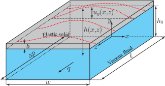
Figure 1: Schematic illustration of the geometry consisting of a three-dimensional deformable channel of length $\ell$ with an initially rectangular cross-section of width $w$ and height $h_{0}$. The channel contains a viscous fluid steadily driven by an imposed flow rate $q$, leading to the deformation $u_{y}(x,z)$ of the top wall of thickness $b$, which in turn affects the pressure drop $\Delta p$ over the axial distance $\ell$. The sidewalls are assumed to be rigid.

Consider the incompressible steady pressure-driven flow of a Newtonian viscous fluid in a slender and deformable channel of length $\ell$, width $w$, and (deformed) height $h$, as shown in Fig. 1. The fluid flow has velocity $\bm{v}=(v_{x},v_{y},v_{z})$ and pressure distribution $p$, which are induced by the imposed flow rate $q$. Our goal is to determine the resulting axial pressure drop $\Delta p$ for a given $q$. The top wall of the channel is soft and may deform due to the fluid stress distribution, acting at the fluid–solid interface, leading to the displacement field $\bm{u}=(u_{x},u_{y},u_{z})$. The sidewalls are assumed to be rigid. Specifically, we use $u_{y}^{0}(x,z)$ to denote the steady vertical displacement of the lower surface of the top wall, i.e., the fluid–solid interface, so that its position is given by $y=h(x,z)=h_{0}+u_{y}^{0}(x,z)$, where $h_{0}$ is the undeformed height of the channel (in the absence of flow). We further assume the top wall of the channel has a constant thickness $b$ and constant material properties.

We consider low-Reynolds-number flow, so that fluid inertia is negligible compared to viscous forces. In this limit, the continuity and momentum equations governing the fluid motion take the form

$$\bm{\nabla\cdot v}=0,\qquad\bm{\nabla\cdot}\bm{\sigma}_{f}=\bm{0},$$ (1)

where $\bm{\sigma}_{f}=-p\bm{I}+\mu(\bm{\nabla}\bm{v}+(\bm{\nabla}\bm{v})^{\mathrm{T}})$ is the Newtonian stress tensor, $\bm{I}$ is the identity tensor, and $\mu$ is the fluid’s dynamic viscosity. The governing equations (1) are supplemented by the no-slip and no-penetration boundary conditions along the channel walls, $\bm{v}=\bm{0}$ at $y=0,\,h(x,z)$, and at $x=\pm w/2$. Further, the integral constraint $\int_{-w/2}^{w/2}\int_{0}^{h(x)}v_{z}(x,y,z)\,\mathrm{d}y\,\mathrm{d}x=q$ enforces the flow rate. In addition, we assume that fluid exits at the outlet to atmosphere and set $p(\ell)=0$, so that $\Delta p=p(0)$.

Suppose that the top wall of the channel can be modeled as a linearly elastic isotropic solid with shear modulus $G$ and first Lamé parameter $\lambda$. Neglecting body forces in the solid, the steady stress balance in the elastic material takes the form

$$\bm{\nabla\cdot\sigma}_{s}=\bm{0},$$ (2)

where $\bm{\sigma}_{s}=\lambda(\bm{\nabla\cdot}\bm{u})\bm{I}+2G\bm{D}$ is the stress tensor of a linearly elastic solid and $\bm{D}=(\bm{\nabla}\bm{u}+(\bm{\nabla}\bm{u})^{\mathrm{T}})/2$ is the infinitesimal strain tensor. Note that $G$ and $\lambda$ are related to the Young’s modulus $E$ and Poisson’s ratio $\nu$ as $G=E/[2(1+\nu)]$ and $\lambda=E\nu/(1+\nu)(1-2\nu)$. The governing equation (2) is supplemented by the no-displacement boundary condition, $\bm{u}=\bm{0}$ along the lines of contact, $z=0,\,\ell$, and $x=\pm w/2$, with the inlet/outlet and rigid walls. In addition, at the fluid–solid interface $y=h(x,z)$, the continuity of stresses requires that $\bm{n}\bm{\cdot}\bm{\sigma}_{s}=\bm{n}\bm{\cdot}\bm{\sigma}_{f}$, where $\bm{n}$ is the unit normal vector to the fluid–solid interface. This condition couples the fluidic and elastic problems. Finally, we assume a stress-free condition at the upper surface of the top wall, i.e., $\tilde{\bm{n}}\bm{\cdot}\bm{\sigma}_{s}=\bm{0}$, where $\tilde{\bm{n}}$ is the unit normal vector to the upper surface of the soft wall.

We introduce dimensionless variables based on lubrication theory,

$$X=\frac{x}{w},\quad Y=\frac{y}{h_{0}},\quad Z=\frac{z}{\ell},\quad V_{x}=\frac{v_{x}}{(\epsilon/\delta)v_{c}},\quad V_{y}=\frac{v_{y}}{\epsilon v_{c}},\quad V_{z}=\frac{v_{z}}{v_{c}},\quad P=\frac{p}{p_{c}},\quad H=\frac{h}{h_{0}},\quad U=\frac{u_{y}}{u_{c}},$$ (3)

where $v_{c}=q/(h_{0}w)$ is the characteristic axial velocity scale, $p_{c}=\mu v_{c}\ell/h_{0}^{2}=\mu q\ell/(wh_{0}^{3})$ is the characteristic pressure scale, and $u_{c}$ is the characteristic scale of deformation of the top wall Christov et al. (2018). Also, we have defined $\epsilon=h_{0}/\ell$ and $\delta=h_{0}/w$, which represent, respectively, the slenderness and the shallowness of the channel. We assume $\epsilon=h_{0}/\ell$ to be small, $\epsilon\ll 1$, but $\delta=h_{0}/w$ can be $\mathrm{O}(1)$, with the ordering $0<\epsilon\ll\mathrm{min}(\delta,1)$. Thus, unlike previous theoretical studies that assumed $\delta=h_{0}/w\ll 1$ Christov et al. (2018); Shidhore and Christov (2018); Mehboudi and Yeom (2019); Wang and Christov (2019); Martínez-Calvo et al. (2020); Ramos-Arzola and Bautista (2021), we consider a slender channel that is not necessarily shallow.

In recent studies it was shown that for rectangular elastic top wall geometries, the horizontal displacements $u_{x}$ and $u_{z}$ are much smaller in comparison to the vertical displacement $u_{y}$ Wang and Christov (2019). The latter can also be rationalized using a scaling argument. Balancing the elastic elongational stress and the viscous stress at the top wall, we obtain that $u_{z}$ scales as $\mu q\ell/(Ewh_{0}^{2})$. Thus, for example, for the plate-bending theory in which $b\ll w$ and $u_{y}\sim\mu q\ell w^{3}/(Eb^{3}h_{0}^{3})$, we find $u_{z}/u_{y}\sim b^{3}h_{0}/w^{4}\ll 1$. A similar argument yields $u_{x}/u_{y}\ll 1$. Therefore, it is sufficient and convenient, to consider that the entire deformation of the top wall is in the $y$-direction. Further, for thin structures $b\lesssim w$, the deformation at the fluid–solid interface is representative of the entire wall motion (i.e., $u_{y}\approx u_{y}^{0}$), consistent with reduced theories of elastic deformation, such as those due to Winkler, Kirchhoff–Love, Mindlin–Reissner, and Föppl–von Kármán Timoshenko and Woinkowsky-Krieger (1987); Howell et al. (2009). Therefore, in the following, we make explicit the kinematic assumption that the displacement of the fluid–solid interface can be written as $\bm{u}=(0,u_{y}(x,z),0)$. Thus, the dimensionless deformed shape of the channel $H(X,Z)$ can be expressed in terms of the dimensionless top wall deformation $U(X,Z)$ as

$$H(X,Z)=1+(u_{c}/h_{0})U(X,Z)=1+\beta U(X,Z),$$ (4)

where $\beta=u_{c}/h_{0}$ is the dimensionless ratio that quantifies the compliance of the top wall.

III Reciprocal theorems for viscous flows in weakly deformable channels

III.1 Fluidic reciprocal theorem

Let $\hat{\bm{v}}$, $\hat{p}$, and $\hat{\bm{\sigma}}_{f}$ denote, respectively, the velocity, pressure, and stress fields corresponding to the solution of the pressure-driven flow in a rigid (rectangular) channel, satisfying $\bm{\nabla\cdot}\hat{\bm{v}}=0$, $\bm{\nabla\cdot}\hat{\bm{\sigma}}_{f}=\bm{0}$, with $\hat{\bm{\sigma}}_{f}=-\hat{p}\bm{I}+\mu(\bm{\nabla}\hat{\bm{v}}+(\bm{\nabla}\hat{\bm{v}})^{\mathrm{T}})$. To exploit the reciprocal theorem, we first expand the velocity, pressure, and stress fields into perturbation series in the dimensionless parameter $\beta=u_{c}/h_{0}\ll 1$ controlling the compliance of the top wall:

$$\bm{v} =\hat{\bm{v}}+\beta\bm{v}_{1}+\mathrm{O}(\beta^{2}),$$ (5a)

$$p =\hat{p}+\beta p_{1}+\mathrm{O}(\beta^{2}),$$ (5b)

$$\bm{\sigma}_{f} =\hat{\bm{\sigma}}_{f}+\beta\bm{\sigma}_{f,1}+\mathrm{O}(\beta^{2}),$$ (5c)

where $\bm{v}_{1}$, $p_{1}$, and $\bm{\sigma}_{f,1}$ are the first-order corrections to the velocity, pressure, and hydrodynamic stress in the rectangular domain due to the deformation of the top wall. From (1) and (5), it follows that the corresponding governing equations are the Stokes equations $\bm{\nabla\cdot}\bm{v}_{1}=0$, $\bm{\nabla\cdot}\bm{\sigma}_{f,1}=\bm{0}$. The Lorentz reciprocal theorem states that the two sets of velocity and stress fields $(\hat{\bm{v}},\hat{\bm{\sigma}}_{f})$ and $(\bm{v}_{1},\bm{\sigma}_{f,1})$ satisfy Happel and Brenner (1983):

$$\int_{S_{0}}\bm{n}\bm{\cdot}\bm{\sigma}_{f,1}\bm{\cdot}\hat{\bm{v}}\,\mathrm{d}S+\int_{S_{\ell}}\bm{n}\bm{\cdot}\bm{\sigma}_{f,1}\bm{\cdot}\hat{\bm{v}}\,\mathrm{d}S+\underbrace{\int_{S_{\mathrm{top}}}\bm{n}\bm{\cdot}\bm{\sigma}_{f,1}\bm{\cdot}\hat{\bm{v}}\,\mathrm{d}S}_{=0}=\int_{S_{0}}\bm{n}\bm{\cdot}\hat{\bm{\sigma}}_{f}\bm{\cdot}\bm{v}_{1}\,\mathrm{d}S+\int_{S_{\ell}}\bm{n}\bm{\cdot}\hat{\bm{\sigma}}_{f}\bm{\cdot}\bm{v}_{1}\,\mathrm{d}S+\int_{S_{\mathrm{top}}}\bm{n}\bm{\cdot}\hat{\bm{\sigma}}_{f}\bm{\cdot}\bm{v}_{1}\,\mathrm{d}S,$$ (6)

where $S_{\mathrm{top}}$ is the lower surface of the top wall in the undeformed state, $S_{0}$ and $S_{\ell}$ are the surfaces at the inlet ($z=0$) and outlet ($z=\ell$), respectively, and $\bm{n}$ is the unit outward normal on a respective surface. Note that the integrals over the bottom and side walls of the channel vanish because $\hat{\bm{v}}=\bm{v}_{1}=\bm{0}$ there. Also, the last term on the left-hand side of (6) vanishes because $\hat{\bm{v}}=\bm{0}$ on $S_{\mathrm{top}}$.

Using the asymptotic expansion (5) and non-dimensionalization (3), we obtain

$$\left.\bm{n}\bm{\cdot}\bm{\sigma}_{f,1}\bm{\cdot}\hat{\bm{v}}\right|_{z=0,\,\ell}=\mp\frac{\mu v_{c}^{2}\ell}{h_{0}^{2}}\left[-P_{1}\hat{V}_{z}+\mathrm{O}(\beta)\right]_{Z=0,\,1},\qquad\left.\bm{n}\bm{\cdot}\hat{\bm{\sigma}}_{f}\bm{\cdot}\bm{v}_{1}\right|_{z=0,\,\ell}=\mp\frac{\mu v_{c}^{2}\ell}{h_{0}^{2}}\left[-\hat{P}V_{z,1}+\mathrm{O}(\beta)\right]_{Z=0,\,1},$$ (7)

where the minus sign in (7) corresponds to $S_{0}$ and the plus sign corresponds to $S_{\ell}$ (see Boyko and Stone (2021, 2022)).

Similarly, the integrand in the last term of (6), evaluated at $y=h_{0}$ (i.e., on $S_{\mathrm{top}}$), with $\bm{n}=\bm{e}_{y}$ and $\bm{n}\bm{\cdot}\hat{\bm{\sigma}}_{f}=\mu(\partial\hat{v}_{z}/\partial y)\bm{e}_{z}-\hat{p}\bm{e}_{y}$, is

$$\left.\bm{n}\bm{\cdot}\hat{\bm{\sigma}}_{f}\bm{\cdot}\bm{v}_{1}\right|_{y=h_{0}}=\frac{\mu v_{c}^{2}}{h_{0}}\left[\frac{\partial\hat{V}_{z}}{\partial Y}V_{z,1}\right]_{Y=1}.$$ (8)

Note that the pressure term in $\bm{n}\bm{\cdot}\hat{\bm{\sigma}}_{f}$ does not contribute to (8) because the leading-order flow is purely axial, so that $\left.\bm{v}_{1}\bm{\cdot}\bm{e}_{y}\right|_{y=h_{0}}=0$ due to no penetration. We determine $V_{z,1}(X,Y=1,Z)$ by applying the no-slip boundary condition, $V_{z}(X,Y=H(X,Z),Z)=0$, and using (4) and (5a), together with the domain perturbation expansion in $\beta$ introduced above, to obtain

$$V_{z}(X,H(X,Z),Z)=\hat{V}_{z}(X,1,Z)+\beta\left(V_{z,1}(X,1,Z)+U(X,Z)\left.\frac{\partial\hat{V}_{z}}{\partial Y}\right|_{Y=1}\right)+\mathrm{O}(\beta^{2})=0.$$ (9)

It follows that $V_{z,1}(X,1,Z)=-U(X,Z)\left.\partial\hat{V}_{z}/\partial Y\right|_{Y=1}$. Thus, (8) reduces to

$$\left.\bm{n}\bm{\cdot}\hat{\bm{\sigma}}_{f}\bm{\cdot}\bm{v}_{1}\right|_{y=h_{0}}=\frac{\mu v_{c}^{2}}{h_{0}}\left[\frac{\partial\hat{V}_{z}}{\partial Y}V_{z,1}\right]_{Y=1}=-\frac{\mu v_{c}^{2}}{h_{0}}U(X,Z)\left(\left.\frac{\partial\hat{V}_{z}}{\partial Y}\right|_{Y=1}\right)^{2}+\mathrm{O}(\beta).$$ (10)

Substituting (7) and (10) into (6), and using the outlet boundary condition $P_{1}(Z=1)=\hat{P}(Z=1)=0$, we obtain

$$\int_{0}^{1}\int_{-1/2}^{1/2}\left[P_{1}\hat{V}_{z}-\hat{P}V_{z,1}\right]_{Z=0}\mathrm{d}X\mathrm{d}Y=-\int_{0}^{1}\int_{-1/2}^{1/2}\left[U(X,Z)\left(\left.\frac{\partial\hat{V}_{z}}{\partial Y}\right|_{Y=1}\right)^{2}\right]\mathrm{d}X\mathrm{d}Z+\mathrm{O}(\beta).$$ (11)

Noting that $P_{1}=P_{1}(Z)$ and $\hat{P}=\hat{P}(Z)$ to the leading order in $\epsilon$, consistent with the classical lubrication approximation Leal (2007), and $\int_{0}^{1}\int_{-1/2}^{1/2}\hat{V}_{z}\mathrm{d}X\mathrm{d}Y=1$ and $\int_{0}^{1}\int_{-1/2}^{1/2}V_{z,1}\mathrm{d}X\mathrm{d}Y=0$, (11) yields the first-order correction to the pressure drop, defined as $\Delta P_{1}=P_{1}(Z=0)$, for the weakly deformable channel ($\beta\ll 1$):

$$\Delta P_{1}=-\int_{0}^{1}\int_{-1/2}^{1/2}\left[U(X,Z)\left(\left.\frac{\partial\hat{V}_{z}}{\partial Y}\right|_{Y=1}\right)^{2}\right]\mathrm{d}X\mathrm{d}Z.$$ (12)

Equation (12) is the first key result of this Letter, which allows the determination of the first-order correction to the pressure drop of the deformable channel, provided the top wall deformation $U(X,Z)$ is known. Therefore, in fact, (12) is not restricted to deformable channels, and provides the first-order correction to the pressure drop for the three-dimensional rigid channel, whose top wall is non-uniform and has any prescribed shape variation expressed as $H(X,Z)=1+\beta U(X,Z)$.

III.2 Elastic reciprocal theorem

Let $\tilde{\bm{u}}$ and $\tilde{\bm{\sigma}}_{s}$ denote, respectively, the displacement and stress fields corresponding to the solution of the elastic problem in the same domain but with different boundary conditions on the stress or displacement fields. The corresponding governing equation is $\bm{\nabla\cdot}\tilde{\bm{\sigma}}_{s}=\bm{0}$, with $\tilde{\bm{\sigma}}_{s}=\lambda(\bm{\nabla\cdot}\tilde{\bm{u}})\bm{I}+2G\tilde{\bm{D}}$. The Maxwell–Betti reciprocal theorem Betti (1872); Maxwell (1864); Achenbach (2003) states that the solutions, $(\bm{u},\bm{\sigma}_{s})$ and $(\tilde{\bm{u}},\tilde{\bm{\sigma}}_{s})$, to the two elastostatic problems satisfy:

$$\int_{S}\bm{n}\bm{\cdot}\bm{\sigma}_{s}\bm{\cdot}\tilde{\bm{u}}\,\mathrm{d}S=\int_{S}\bm{n}\bm{\cdot}\tilde{\bm{\sigma}}_{s}\bm{\cdot}\bm{u}\,\mathrm{d}S,$$ (13)

where $\bm{n}$ is the unit outward normal to the bounding surfaces $S$ of the elastic solid.

Before applying the elastic reciprocal theorem (13) to our elastohydrodynamic problem, recall a few assumptions we have made. First, in this problem, $\bm{u}=u_{y}(x,z)\bm{e}_{y}$ and $\tilde{\bm{u}}=\tilde{u}_{y}(x,z)\bm{e}_{y}$. Second, there is no-displacement on the lateral walls of the solid. Third, the continuity of tractions, $\bm{n}\bm{\cdot}\bm{\sigma}_{s}=\bm{n}\bm{\cdot}\bm{\sigma}_{f}$, holds at the fluid$-$solid interface, $y=h(x,z)$. Lastly, we have assumed a stress-free condition at the upper surface of the top wall. Based on these assumptions, the terms, $\bm{n}\bm{\cdot}\bm{\sigma}_{s}\bm{\cdot}\tilde{\bm{u}}$ and $\bm{n}\bm{\cdot}\tilde{\bm{\sigma}}_{s}\bm{\cdot}\bm{u}$, appearing in (13) are calculated as

$$\left.\bm{n}\bm{\cdot}\bm{\sigma}_{s}\bm{\cdot}\tilde{\bm{u}}\right|_{y=h(x,z)}=\left.\bm{n}\bm{\cdot}\bm{\sigma}_{f}\bm{\cdot}\tilde{\bm{u}}\right|_{y=h(x,z)}=p_{c}u_{c}\left[-P\tilde{U}+\mathrm{O}(\epsilon)\right]=p_{c}u_{c}\left[-\hat{P}\tilde{U}+\mathrm{O}(\epsilon,\beta)\right],$$ (14a)

$$\left.\bm{n}\bm{\cdot}\tilde{\bm{\sigma}}_{s}\bm{\cdot}\bm{u}\right|_{y=h(x,z)}=\left.\bm{n}\bm{\cdot}\tilde{\bm{\sigma}}_{f}\bm{\cdot}\bm{u}\right|_{y=h(x,z)}=p_{c}u_{c}\left[-\tilde{P}U+\mathrm{O}(\epsilon)\right]=p_{c}u_{c}\left[-\hat{\tilde{P}}U+\mathrm{O}(\epsilon,\beta)\right],$$ (14b)

where to obtain the last equality we used the domain perturbation expansion introduced above, i.e., $P=\hat{P}+\mathrm{O}(\beta)$ and $\tilde{P}=\hat{\tilde{P}}+\mathrm{O}(\beta)$. Substituting (14) into (13) leads to

$$\int_{0}^{1}\int_{-1/2}^{1/2}\hat{\tilde{P}}U\,\mathrm{d}X\mathrm{d}Z=\int_{0}^{1}\int_{-1/2}^{1/2}\hat{P}\tilde{U}\,\mathrm{d}X\mathrm{d}Z.$$ (15)

Next, we utilize the convolution principle to obtain an explicit expression for the deformation $U(X,Z)$ from (15). Choosing $\hat{\tilde{P}}$ as a point load, i.e., $\hat{\tilde{P}}=\delta_{D}(X-\mathcal{X})\delta_{D}(Z-\mathcal{Z})$, applied on the fluid–solid interface at the point $(\mathcal{X},\mathcal{Z})$, where $\delta_{D}$ is the Dirac delta distribution, we obtain

$$U(X,Z)=\int_{0}^{1}\int_{-1/2}^{1/2}\hat{P}(\mathcal{X},\mathcal{Z})\tilde{U}(X,Z;\mathcal{X},\mathcal{Z})\,\mathrm{d}\mathcal{X}\mathrm{d}\mathcal{Z}.$$ (16)

Here, $\tilde{U}(X,Z;\mathcal{X},\mathcal{Z})$ is the point-load solution (or, Green’s function) of the elastic problem with appropriate boundary conditions under the aforementioned assumptions.

III.3 Flow rate–pressure drop relation for deformable channels using fluidic and elastic reciprocal theorems

Combining (12) and (16), we obtain the first-order correction to the pressure drop for the weakly deformable channel, $\beta\ll 1$, expressed using the fluidic and elastic reciprocal theorems:

$$\Delta P_{1}=-\int_{0}^{1}\int_{-1/2}^{1/2}\left[\int_{0}^{1}\int_{-1/2}^{1/2}\hat{P}(\mathcal{X},\mathcal{Z})\tilde{U}(X,Z;\mathcal{X},\mathcal{Z})\,\mathrm{d}\mathcal{X}\mathrm{d}\mathcal{Z}\left(\left.\frac{\partial\hat{V}_{z}}{\partial Y}\right|_{Y=1}\right)^{2}\right]\mathrm{d}X\mathrm{d}Z.$$ (17)

Equation (17) is the second key result of this Letter, clearly indicating that the first-order correction to the pressure drop arises due to the interplay between the fluid stresses and the compliance of the channel. Furthermore, (17) shows that $\Delta P_{1}$ depends only on the solution of the pressure-driven flow in a rigid channel for the fluid problem (hat) and the solution of the elastic deformation for a point-load (tilde), thus eliminating the need to a priori solve the coupled elastohydrodynamic problem.

The dimensionless pressure drop is thus $\Delta P=\Delta\hat{P}+\beta\Delta P_{1}+\mathrm{O}(\beta^{2})$, where the solution of the corresponding pressure-driven flow in a rigid (rectangular) channel Bruus (2008) is well known:

$$\hat{P}(Z)=\frac{12}{1-\kappa(\delta)}(1-Z),\qquad\Delta\hat{P}=\frac{12}{1-\kappa(\delta)},\qquad\text{where}\;\;\kappa(\delta)=\frac{192}{\pi^{5}}\sum_{n=1}^{\infty}\frac{1}{(2n-1)^{5}}\delta\tanh\left[\frac{(2n-1)\pi}{2\delta}\right],$$ (18a)

$$\hat{V}_{z}(X,Y)=\frac{12}{1-\kappa(\delta)}\left[\frac{1}{2}(1-Y)Y-\frac{4}{\pi^{3}}\sum_{n=1}^{\infty}\frac{1}{(2n-1)^{3}}\frac{\cosh[(2n-1)\pi X/\delta]}{\cosh[(2n-1)\pi/(2\delta)]}\sin[(2n-1)\pi Y]\right].$$ (18b)

IV Illustrated example

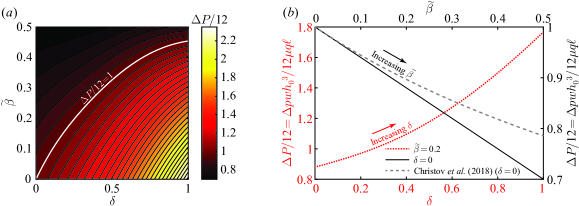
Figure 2: Dimensionless pressure drop $\Delta P/12=\Delta pwh_{0}^{3}/12\mu q\ell$ in a deformable channel modeled using the plate-bending theory. (a) Contour plot of the dimensionless pressure drop as a function of $\tilde{\beta}=u_{c}/24h_{0}$ and $\delta=h_{0}/w$. (b) Dimensionless pressure drop as a function of $\delta=h_{0}/w$ (dotted line) for $\tilde{\beta}=0.2$ and as a function of $\tilde{\beta}=u_{c}/24h_{0}$ (solid and dashed curves) for $\delta=0$. The solid line represents the first-order asymptotic solution and the dashed line represents the solution based on the lubrication theory (also for $\delta=0$), derived by Christov et al. (2018).

In this section, we illustrate an application of our results towards calculating the first-order-in-$\beta$ correction to the pressure drop in a slender compliant channel. For this example and for simplicity, we model the compliance of the top wall using the plate-bending theory. Under the assumptions that the maximum displacement of the top wall is small compared to its thickness $b$, and the thickness $b$ is small compared to its width $w$, $\max_{x,z}[u_{y}(x,z)]\ll b\ll w$, the steady-state displacement $u_{y}(x,y)$ satisfies the Kirchhoff–Love equation for isotropic bending of a plate under a transverse load supplied by the fluid pressure, i.e., $p=B\nabla_{\|}^{4}u_{y}$ Love (1888); Timoshenko and Woinkowsky-Krieger (1987); Howell et al. (2009). Here, $B=Eb^{3}/[12(1-\nu^{2})]$ is the bending stiffness, and $\nabla_{\|}^{4}$ is the biharmonic operator in the $(x,z)$ plane.

Using (3) and performing order-of-magnitude analysis, we obtain $u_{c}=w^{4}p_{c}/B=w^{3}\mu q\ell/(h_{0}^{3}B)$ and thus $\beta=u_{c}/h_{0}=w^{4}p_{c}/(Bh_{0})=w^{3}\mu q\ell/(h_{0}^{4}B)$. Furthermore, it follows that $P(Z)=\partial^{4}U/\partial X^{4}+\mathrm{O}(\epsilon^{2}/\delta^{2})$ Christov et al. (2018); Martínez-Calvo et al. (2020), where $0\ll\epsilon\ll\mathrm{min}(1,\delta)$ but $\delta=h_{0}/w$ is not necessary small. The Green’s function corresponding to the point-load solution of the latter equation with clamped boundary conditions Duffy (2015), i.e., $U|_{X=\pm 1/2}=\left.\partial U/\partial X\right|_{X=\pm 1/2}=0$, is

$$\tilde{U}(X,Z;\mathcal{X},\mathcal{Z})=\frac{1}{24}\left(X-\frac{1}{2}\right)^{2}\left(X+\frac{1}{2}\right)^{2}\delta_{D}(Z-\mathcal{Z}).$$ (19)

Using (18) and (19), (17) provides the first-order correction to the pressure drop for arbitrary value of $\delta=h_{0}/w$. We note that it is difficult to obtain a closed-form expression for $\Delta P_{1}$, which holds for any $\delta=h_{0}/w$, because of the velocity profile (18b) is represented as an infinite series. While the $Z$-integration can be performed analytically, the $X$-integration is done numerically. However, for $\delta\ll 1$, from (18b) it follows that $\Delta\hat{P}=12$, $\hat{P}(Z)=12(1-Z)$, and $\hat{V}_{z}(Y)=6(1-Y)Y$, and substituting theses results and (19) into (17) yields $\Delta P_{1}/12=-3/120$, so that $\Delta P/12=1-(3/120)\beta+\mathrm{O}(\beta^{2})=1-(3/5)\tilde{\beta}+\mathrm{O}(\tilde{\beta}^{2})$, where $\tilde{\beta}=\beta/24=w^{4}p_{c}/(24Bh_{0})=w^{3}\mu q\ell/(24h_{0}^{4}B)$.

It is instructive to compare the latter result to the solution for the dimensionless pressure drop previously derived by Christov et al. (2018) using lubrication theory. The result from Christov et al. (2018), holding for $\delta\ll 1$ and $\tilde{\beta}=\mathrm{O}(1)$, is expressed as an implicit relation:

$$12=\Delta P\left[1+\frac{\tilde{\beta}}{20}\Delta P+\frac{\tilde{\beta}^{2}}{630}(\Delta P)^{2}+\frac{\tilde{\beta}^{3}}{48048}(\Delta P)^{3}\right]\qquad(\mathrm{lubrication\,theory\,for}\,\delta\ll 1),$$ (20)

and it also yields $\Delta P/12=1-(3/5)\tilde{\beta}+(86/175)\tilde{\beta}^{2}+\mathrm{O}(\tilde{\beta}^{3})$ for $\beta\ll 1$, upon solving for the positive real root of (20). Observe that this expression is identical to our asymptotic solution for the pressure drop to first order in $\tilde{\beta}$.

In Fig. 2(a), we present a contour plot of the dimensionless pressure drop accounting for the first-order correction due to fluid–structure interaction as a function of $\tilde{\beta}=u_{c}/24h_{0}$ and $\delta=h_{0}/w$, for the deformable channel modeled using the plate-bending theory. Figure 2(a) clearly indicates the existence of the trade-off between the effect of compliance of the deforming top wall and the effect of sidewalls on the pressure drop. While the pressure drop decreases with $\tilde{\beta}$, it increases with $\delta$. The white (light) solid curve $\Delta P/12=1$ divides the colormap into two regions: in the upper region, the compliance dominates over the sidewall effects and thus $\Delta P/12<1$, whereas in the lower region, the sidewall drag is dominant and $\Delta P/12>1$.

Next, in Fig. 2(b), we show a comparison of our analytical predictions and the lubrication-theory-based solution (20) for the non-dimensional pressure drop as a function of $\tilde{\beta}$, for $\delta=0$ (an infinitely wide channel). The black solid line represents our first-order asymptotic solution, $\Delta P/12=1-(3/5)\tilde{\beta}+\mathrm{O}(\tilde{\beta}^{2})$, and the gray dashed curve represents the lubrication solution, (20). It is evident from Fig. 2(b) that our first-order asymptotic solution, which is strictly valid for $\tilde{\beta}\ll 1$, slightly underpredicts the lubrication solution; yet even for $\tilde{\beta}=0.5$, it results in a modest relative error of approximately 10$\%$. For further clarification, the dotted (red) curve shows the dimensionless pressure drop as a function of $\delta=h_{0}/w$, for $\tilde{\beta}=0.2$, clearly indicating that, while increased wall compliance decreases the pressure drop, drag due to the sidewalls increases it.

V Concluding remarks

In this Letter, we showed how the reciprocal theorems for Stokes flow and linear elasticity can be used to derive a closed-form expression for leading-order correction, due to deformation, to the flow rate–pressure drop relation for rectangular channels. Using a domain perturbation approach and considering small deformation, our theory captures the interplay between the fluid stresses and the compliance of the channel’s top wall, bypassing the need to calculate the solution of the coupled fluid-structure-interaction problem. Furthermore, unlike previous theoretical studies, which neglected the presence of lateral sidewalls (and considered shallow geometries of effectively infinite width within the lubrication approximation), our approach allows the determination of the influence of confining sidewalls on the $q-\Delta p$ relation.

The present theoretical approach is not limited to the case of a three-dimensional channel of initially rectangular cross-section, and it could also be applied to calculate the first-order correction to the pressure drop in axisymmetric deformable tubes, for which the leading-order pressure drop is given by the classical Hagen–Poiseuille law Sutera and Skalak (1993). Finally, while we considered viscous Newtonian fluids, it would be of interest to understand how the rheological response of complex fluids (such as shear thinning and viscoelasticity) influences the flow rate–pressure drop relation in deformable channels. One convenient approach to accomplish this task would be to rely on reciprocal theorems, and use a combination of the present approach and the approach recently established by Boyko and Stone (2021, 2022) for calculating the effect of complex fluid rheology on the flow rate–pressure drop relation for rigid non-uniform channels. These calculations are left for future investigation.