Equilibrium properties of the lattice fluid with the repulsion between the nearest neighbors on the two-level lattice with nonrectangular geometry

Abstract

The equilibrium properties of the lattice fluid with the repulsion between the nearest neighbors on the two-level planar triangular lattice are investigated. The numerical results obtained from the analytical expressions are compared with the Monte Carlo simulation data. It is shown that the previously proposed diagrammatic approximation makes it possible to determine the equilibrium characteristics of the lattice fluid with the repulsion between the nearest neighbors on a two-level lattice with an accuracy comparable to the accuracy of modelling the system using the Monte Carlo method in the entire range of thermodynamic parameters. It was found that, in contrast to a similar one-level system, a lattice fluid with the repulsion between the nearest neighbors undergoes a first-order phase transition.

Key words: lattice fluid, two-level lattice, quasi-chemical approximation, diagram approximation, Monte Carlo simulation

Abstract

Äîñëiäæóþòüñÿ ðiâíîâàæíi âëàñòèâîñòi ґðàòêîâîãî ôëþ¿äó ç âiäøòîâõóâàííÿì ìiæ íàéáëèæчèìè ñóñiäàìè íà äâîõðiâíåâié ïëîñêié òðèêóòíié ґðàòöi. Чèñëîâi ðåçóëüòàòè, îòðèìàíi ç àíàëiòèчíèõ âèðàçiâ, ïîðiâíþþòüñÿ ç äàíèìè ìîäåëþâàííÿ Ìîíòå-Êàðëî. Ïîêàçàíî, ùî çàïðîïîíîâàíå ðàíiøå äiàãðàìíå íàáëèæåííÿ äàє ìîæëèâiñòü âèçíàчèòè ðiâíîâàæíi õàðàêòåðèñòèêè ґðàòêîâîãî ôëþ¿äó ç âiäøòîâõóâàííÿì ìiæ íàéáëèæчèìè ñóñiäàìè íà äâîõðiâíåâié ґðàòöi ç òîчíiñòþ, ïîäiáíîþ äî òîчíîñòi ìîäåëþâàííÿ ñèñòåìè ç âèêîðèñòàííÿì ìåòîäó Ìîíòå-Êàðëî, â öiëîìó äiàïàçîíi òåðìîäèíàìiчíèõ ïàðàìåòðiâ. Âèÿâëåíî, ùî íà âiäìiíó âiä ïîäiáíî¿ îäíîðiâíåâî¿ ñèñòåìè, ґðàòêîâèé ôëþ¿ä ç âiäøòîâõóâàííÿì ìiæ íàéáëèæчèìè ñóñiäàìè çàçíàє ôàçîâîãî ïåðåõîäó ïåðøîãî ðîäó.

Ключовi слова: ґðàòêîâèé ôëþ¿ä, äâîðiâíåâà ґðàòêà, êâàçiõiìiчíå íàáëèæåííÿ, äiàãðàìíå íàáëèæåííÿ, ìîäåëþâàííÿ Ìîíòå-Êàðëî

Introduction

The model of the lattice gas or the lattice liquid is widely used in the description of processes occurring on the surfaces and in the volumes of solids [1], as well as in the study of various electrochemical systems [2, 3, 4, 5, 6].

The main idea of this model consists in the decomposition of the original physical system into two spatial interpenetrating subsystems, one of which is rather rigidly structured and plays the role of the reference one, and in the second one the particles retain high mobility. In fact, the particles of the second subsystem move in the field created by the supporting subsystem. In this case, it is assumed that the given field does not depend on the distribution of the moving particles. Thus, it can be argued that the reference subsystem creates a potential with a spatially periodic profile for the moving particles, in which there are sufficiently deep potential energy minima that form one or other periodic lattice.

Another condition for the possibility of using the lattice fluid model to describe a real physical system is the presence of two significantly different time scales. The first of which, $\tau_{1}$, is determined by the average residence time of the mobile particle in the minimum of potential energy, and the second, $\tau_{2}$, is determined by the oscillation period of the mobile particle near this position. Hence, for the indicated time scales, we have $\tau_{1}\gg\tau_{2}$.

The fulfillment of the above conditions, the stability of the reference system and the presence of two significantly different time scales, allows us to restrict ourselves to considering only the subsystem of moving particles, and the characteristics of the potential landscape can be considered as the input parameter of the model, assuming them to be given.

The potential energy minima will be determined as the lattice sites, each of which can be either occupied by a single particle or can be vacant. When considering a system of charged particles occupying the lattice sites, the number of possible states of each lattice site obviously increases [7] in comparison with the case of uncharged particles. In the case of a system with charged particles, each lattice site can be occupied by a positive particle, a negative particle, or can be vacant.

One of the ways for the development of lattice models is the transition to the lattice models with energetically nonequivalent lattice sites. For example, the so-called two-level system in which the nodes of two different types are present can be considered.

Earlier in the literature, several versions of two-level models of the lattice fluid were presented [3, 4, 5, 8, 9, 10, 11, 12]. For example, the models with a random distribution of energetically deeper and shallower nodes were proposed [3, 4, 8, 10], as well as the models, in which the nodes of different types form some symmetrical structures [3, 9, 11, 12]. In the latter case, it was shown [5, 6] that the model of a lattice fluid on a two-dimensional two-level lattice can be used to study layered intercalation compounds, for example, graphite intercalated with lithium ions. In case of such systems, the typical values of deep level energies are of the order of several tenths of eV, while shallow level energies can be considerably lower or comparable with the former. In many cases, interparticle interactions are of the order of several hundredths of eV.

In [12, 13], the lattice fluid on the 2D rectangular two-level lattice was investigated using a decoration-iteration transformation, which made it possible to reduce the problem to considering a lattice gas on a homogeneous square lattice, and investigating the type of the phase diagram. In particular, by means of real-space renormalization group (RSRG) method it was established [13] that in the considered system with repulsion between the nearest neighbors the first-order phase transition takes place. This is a quite unusual phase transition of the first order in a lattice gas system with mutual repulsion between adparticles. The existence of the first-order phase transition was also confirmed with the help of Monte Carlo (MC) simulation [12]. Moreover, in [12] the equilibrium properties of the lattice fluids with interaction between nearest neighbors on the rectangular two-level lattice were investigated with the help of RSRG method and MC simulation.

The diffusion properties of this model were studied using the Monte Carlo simulation method [14, 15, 16, 17, 18, 19, 20, 21]. It can also be noted that the number of approximate methods belonging to the class of mean field methods were developed to determine the equilibrium properties of this system [22]. Within the framework of the constructed approximate approaches, the thermodynamic, structural and transport properties of systems with repulsion and attraction between nearest neighbors [23] on a square lattice were investigated.

In this article we consider the possibility of constructing approximate approaches for assessing the equilibrium properties of the lattice fluid on the lattice with non-rectangular geometry. The quasi-chemical (QChA) and diagram (DA) approximations will be developed to estimate the equilibrium properties of the two-level lattice system based on the planar triangular lattice. The accuracy of both approximations will be verified by comparing the QChA and DA results with the Monte Carlo (MC) simulations data. Furthermore, within the framework of the two approaches, mean field approximations and MC, the equilibrium properties of the lattice fluid with the repulsive interaction between the nearest neighbors on the two-level lattice will be investigated.

1 Model

The crystal plane (1, 1, 1) of the crystal with the simple cubic Bravais lattice can be considered as the basis for constructing a two-level lattice system. In this plane, the atoms of the crystal form a triangular lattice as shown in figure 1, where these atoms are represented by open squares. The interaction between the atoms of the plane forms an energy profile, the minima of which are the locations of the particles adsorbed on a given plane of the crystal, the so-called adparticles. The ensemble of these adparticles forms the system under study.

The geometric features of the original lattice make it possible to distinguish two types of sites of the lattice model. Some of them — $\alpha$-sites — are located between two neighboring atoms of the crystal plane and are shown in figure 1 with open circles. The second type of sites — $\gamma$-sites — are in the center of the regular triangle built on three neighboring atoms. In figure 1, $\gamma$-sites are shown as closed circles.

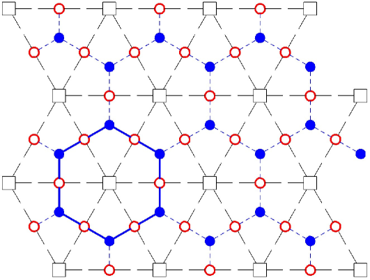
Figure 1: (Colour online) Schematic view of the lattice with two types of sites. The open squares correspond to the atoms of the crystal plane (1, 1, 1), the open and closed circles correspond to the $\alpha$- and $\gamma$-sites of the lattice model.

In the general case, the depths of potential wells corresponding to the $\alpha$- and $\gamma$-sites can be different

$$\epsilon_{\alpha}\neq\epsilon_{\gamma},\quad\delta\epsilon=\epsilon_{\alpha}-\epsilon_{\gamma},$$ (1.1)

where $\epsilon_{\alpha}$, $\epsilon_{\gamma}$ denote the depth of the potential well corresponding to the lattice sites of the indicated type, and $\delta\epsilon$ is the difference in the depths of the potential wells.

Since the $\alpha$ and $\gamma$ sites are not energetically equivalent, the probability of finding the particle in each of them can be different. For a theoretical description of this system, the original lattice can be divided into the system of two sublattices, each of which contains the sites of only one type. This allows us to speak in what follows about the $\alpha$ and $\gamma$ sublattices, respectively.

Thus, the constructed lattice system is a combination of two two-dimensional hexagonal sublattices. In this case, the $\alpha$-sublattice has a lattice constant $a/2$, and the $\gamma$-sublattice has a lattice constant $a/\sqrt{3}$, where $a$ is the distance between the atoms of the crystal plane.

It can also be noted that the first coordination number, i.e., the number of the nearest neighbor nodes is different for the sublattices introduced above. Thus, for example, the sublattice site $\alpha$ has $z_{\alpha}=2$ nearest-neighbor sites. Moreover, all these nearest neighboring sites belong to the $\gamma$ sublattice. On the other hand, for a $\gamma$-site, the number of nearest sites on the $\alpha$ sublattice is $z_{\gamma}=3$.

In this paper, we consider the lattice fluid with the interaction between nearest neighbors. The energy of this interaction is assumed to be equal to $J_{1}$. It should be noted that the particles occupying the lattice sites of the same type do not interact with each other, because these nodes are not nearest neighbors.

Counting the sites on each of the sublattices is not difficult. As noted above, the $\alpha$-site is located between every two nearest atoms of the crystal plane. If we assume that the initial crystal plane contains $M$ atoms forming the triangular lattice with the first coordination number $z_{M}=6$, then the number of pairs of nearest atoms, and hence the number of $\alpha$-sites, is

$$N_{\alpha}=\frac{z_{M}M}{2}.$$ (1.2)

The $\gamma$-site lies in turn in the center of each triangular graph built on triples of the nearest atoms. The method for calculating the corresponding weight coefficients, meaning the number of different graphs of a given type that can be built on the lattice of the selected type, is described in detail in [22]. The weighting coefficient of the three-vertex graph on the triangular lattice, and hence the number of $\gamma$-nodes, is

$$N_{\gamma}=2M.$$ (1.3)

Thus, in the case of a lattice containing $N$ lattice sites, we obtain

$$N_{\alpha}=\frac{3}{5}N,\quad N_{\gamma}=\frac{2}{5}N.$$ (1.4)

For further calculations, it is convenient to introduce the average first coordination number $z_{1}$ which has the meaning of the average number of the nearest neighboring sites for an arbitrary lattice node. For the lattice under consideration, the coordination number $z_{1}$ will not be an integer. It can be determined by the following relation

$$z_{1}N=z_{\alpha}N_{\alpha}+z_{\gamma}N_{\gamma},\quad z_{1}=\frac{12}{5}.$$ (1.5)

Thus, the original lattice can be considered as the system of two nonequivalent sublattices built on the same lattice sites. For each of the sublattices, the concentration of particles $c_{1}^{\xi}$, and vacancies $c_{0}^{\xi}$ can be determined, and the order parameter of the model $\delta c$

$$c_{\alpha}=c_{1}^{\alpha}=\frac{n_{\alpha}}{N_{\alpha}},\quad c_{\gamma}=c_{1}^{\gamma}=\frac{n_{\gamma}}{N_{\gamma}},\quad c=c_{1}=\frac{n_{\alpha}+n_{\gamma}}{N},$$ (1.6)

$$\delta c=c_{\gamma}-c_{\alpha},\quad c=\frac{3}{5}c_{\alpha}+\frac{2}{5}c_{\gamma},$$ (1.7)

$$c_{\alpha}=c-\frac{2}{5}\delta c,\quad c_{\gamma}=c+\frac{3}{5}\delta c,$$ (1.8)

$$c_{0}=1-cz_{1},\quad c_{0}^{\xi}=1-c_{1}^{\xi},\quad\xi=\alpha,\gamma,$$ (1.9)

where $n_{\xi}$ ($\xi=\alpha,\gamma$) is the number of adparticles on the sublattice $\xi$, and $c_{i}$ is the average concentration of adparticles ($i=1$) and vacancies ($i=0$) in the system.

The thermodynamic state of the constructed lattice model can be defined by specifying the set of occupation numbers $n_{i}$ taking values $n_{i}=1$ or $n_{i}=0$, if the $i$-th lattice site is occupied by the particle or is vacant, respectively.

For a given set of occupation numbers, the potential energy of the system of $n$ particles on the lattice can be represented as:

$$U_{N}=\epsilon_{\alpha}\sum\limits_{\left<\alpha\right>}n_{i}+\epsilon_{\gamma}\sum\limits_{\left<\gamma\right>}n_{i}+\frac{J_{1}}{2}\sum\limits_{\left<nn\right>}n_{i}n_{j},$$ (1.10)

where $\left\langle\alpha\right\rangle$, $\left<\gamma\right>$ and $\left<nn\right>$ denote a summation over all $\alpha$-, $\gamma$-sites and over all pairs of nearest-neighbor sites, respectively.

In what follows, an additional condition will be imposed on the considered lattice system

$$\delta\epsilon=\frac{J_{1}}{2}.$$ (1.11)

Compliance with condition (1.11) ensures the symmetry of the phase diagram around $c=0.5$.

2 Monte Carlo simulation algorithm

Determination of the equilibrium properties of the lattice system can be performed within the framework of the standard Metropolis algorithm [24], the application of which to the lattice fluids of various types is described in detail, for example, in [25, 26, 27, 28].

In this case, the modelling of the equilibrium properties of the system is carried out in the grand canonical ensemble, i.e., with a variable number of particles in the system. Within the framework of this algorithm, the value of the chemical potential $\mu$ and the interaction energy $J_{1}$ is fixed, and the concentration of particles on the lattice $c$ and their distribution are determined directly during the simulation. In this case, the initial distribution of the particles over the $N$-site lattice can be arbitrary.

After choosing an arbitrary lattice site and changing its state (adding a particle if the site is vacant, and removing it if the site is occupied), the change in the energy $\delta E_{N}$ corresponding to the given change in the state of the site is determined as

$$\delta E_{N}=\pm(J_{1}s_{1}-\mu+\epsilon_{\alpha}-\delta\epsilon\delta_{\gamma\xi}),$$ (2.1)

where the plus corresponds to the addition of a particle, and the minus to its removal; $s_{1}$ is the number of particles occupying the nearest lattice sites; $\delta_{\gamma\xi}$ is the Kronecker symbol; index $\xi$ denotes the type of sublattice to which an arbitrarily chosen node belongs.

It should be noted that the maximum number of nearest neighbours for the $\alpha$ and $\gamma$ sublattices are different; i.e., depending on its position, the considered lattice site has a different number of the nearest neighboring nodes. To simplify the program code of the simulation procedure, the lattice system can be supplemented with ghost sites, as shown in figure 2. Ghost lattice sites are represented in this figure by closed squares. In this case, some of the introduced ghost sites coincide in position with the atoms of the crystal plane, which is reflected by the position of the closed squares inside the open ones, representing the atoms of the plane (figure 1).

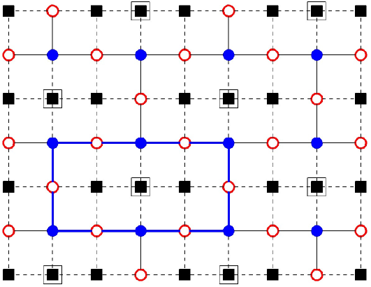
Figure 2: (Colour online) Schematic view of the transformed lattice. Open squares correspond to the atoms of the crystal plane (1, 1, 1), closed squares - to the ghost lattice sites, open and closed circles - to $\alpha$ and $\gamma$-sites of the lattice model, respectively.

The introduction of ghost sites makes it possible to transform the original lattice structure into the “square” lattice, in which each lattice site has 4 nearest neighbors. In this case, any site of the sublattice $\alpha$ will have 2 fictitious sites among its nearest neighbors, and a site of the sublattice $\gamma$ will have only one neighboring ghost site.

Thus, each node of the modelled system $m(i,j)$ can be in one of 3 possible states: $m(i,j)=1$ corresponds to a site $(i,j)$ occupied by the particle, $m(i,j)=0$ — to a vacant lattice site, $m(i,j)=-1$ — to a ghost lattice site. Obviously, during the simulation, the state of the ghost lattice sites does not change. In case of a random choice of the ghost lattice node, the selection procedure is not taken into account and a new node is selected.

If the change in the state of the lattice site leads to a decrease in the energy of the system ($\delta E_{N}\leqslant 0$), then the new configuration is accepted. If the energy of the system increases ($\delta E_{N}>0$), then the change in the state of the site is accepted with the probability

$$W=\exp(-\beta\delta E_{N}),\quad\beta=(k_{\text{B}}T)^{-1},$$ (2.2)

where $T$ is the temperature; $k_{\text{B}}$ is the Boltzmann constant.

In the latter case, to accept or reject the proposed change in the state of the lattice site, a random number $W_{r}$ is generated from the interval $[0;1]$, and if $W\gg W_{r}$, then the new configuration is accepted. Otherwise, the system reverts to its previous state. Repetition of the described procedure of $n$ times, where $n$ is equal to the number of particles on the lattice, forms one step of the Monte Carlo algorithm (MC step).

In this work, the modelled system contains $128\times 128=2^{14}$ lattice sites. Of these, $5\times 2^{11}$ sites are lattice sites of the two-level system, and $3\times 2^{11}$ are the ghost lattice nodes. The complete simulation procedure consists of $30000$ MC steps. Since the modelling procedure begins with a random distribution of particles on the lattice, the first $10000$ MC steps are assigned to the transition of the system from an arbitrary initial state to an equilibrium state and are not taken into account in further modelling. Starting from $10001$ steps of the algorithm, the number of particles in the system, the number of particles on each of the sublattices, and the number of pairs of nearest neighboring sites filled with particles are determined. On the basis of these results, after the end of the modelling procedure, the average concentration of particles in the entire system, the concentration of particles on the sublattices, the order parameter of the system, its thermodynamic factor, and the probability of detecting the two nearest lattice sites with occupied particles.

To reduce the effect of the size of the system on the obtained values of the equilibrium characteristics, we used periodic boundary conditions.

3 Quasi-chemical approximation

Together with the investigated lattice system, a similar reference lattice system can be considered [29, 30, 31]. This reference system is determined by the one-particle average potentials $\phi^{(k)}(n_{i}^{\xi})$ of the interaction of a particle ($n_{i}^{\xi}=1$) or vacancy ($n_{i}^{\xi}=0$) located at site $i$ of the $\xi$-sublattice with some site $j$, which is a neighbor of order $k$ ($\xi=\alpha,\gamma;k=1$ corresponds to nearest neighbors, etc.). The potential energy of the reference system can be as

$$U_{N}^{(0)}=\epsilon_{\alpha}\sum\limits_{\left<\alpha\right>}n_{i}+\epsilon_{\gamma}\sum\limits_{\left<\gamma\right>}n_{i}+\sum\limits_{i=1}^{N}\sum\limits_{k}z_{k}^{\xi}\phi^{(k)}(n_{i}^{\xi}),$$ (3.1)

where $z_{k}^{\xi}$ is the number of neighboring sites of order $k$ for the lattice site of the $\xi$-sublattice. Summation over index $k$ implies summation over the so-called coordination shells, i.e., over complete sets of neighbors of order $k$.

All equilibrium characteristics of the original lattice system are determined by its partition function

$$Q_{N}=\text{Sp}_{\{n_{1}^{\xi},...,n_{N}^{\xi}\}}\{\exp(-\beta U_{N})\},$$ (3.2)

where Sp denotes the summation over all possible particle distributions given by sets of occupation numbers $\{n_{i}^{\xi}\}$, taking into account the normalization conditions

$$n_{\alpha}=\sum\limits_{i=1}^{N_{\alpha}}n_{i}^{\alpha},\quad n_{\gamma}=\sum\limits_{i=1}^{N_{\gamma}}n_{i}^{\gamma},\quad n=n_{\alpha}+n_{\gamma}.$$ (3.3)

The partition function of the initial lattice system (3.2) can be represented as

$$Q_{N} =Q_{N}^{(0)}\text{Sp}_{\{n_{1}^{\xi},...,n_{N}^{\xi}\}}\left\{\exp\left[-\beta\left(U_{N}-U_{N}^{(0)}\right)\right]\frac{\exp(-\beta U_{N}^{(0)})}{Q_{N}^{(0)}}\right\}$$

$$=Q_{N}^{(0)}\left<\exp\left[-\beta\left(U_{N}-U_{N}^{(0)}\right)\right]\right>_{0}=Q_{N}^{(0)}Q_{N}^{(\text{d})},$$ (3.4)

where $Q_{N}^{(0)}$ and $Q_{N}^{(\text{d})}$ are the partition function of the reference system and the diagram part of the partition function, respectively:

$$Q_{N}^{(0)}=\text{Sp}_{\{n_{1}^{\xi},...,n_{N}^{\xi}\}}\left\{\exp\left(-\beta U_{N}^{(0)}\right)\right\},\quad Q_{N}^{(\text{d})}=\left<\exp\left[-\beta\left(U_{N}-U_{N}^{(0)}\right)\right]\right>_{0}.$$ (3.5)

Angular brackets with index 0 denote the averaging over the states of the reference system, the distribution functions of which, due to the one-particle structure of its potential energy, can be written as the product of the average concentrations of particles and vacancies.

The partition function of the reference lattice system can be calculated analytically

$$Q_{N}^{(0)}=\prod\limits_{\xi=\alpha\gamma}\left[\exp(-\beta\epsilon_{\xi}c_{\xi})\prod\limits_{i=0}^{1}\left(\frac{Q_{i}^{\xi}}{c_{i}^{\xi}}\right)^{c_{i}^{\xi}}\right]^{N_{\xi}},\quad Q_{n_{i}^{\xi}}^{\xi}=\exp\left[-\beta\left(\sum\limits_{k}\phi^{(k)}(n_{i}^{\xi})\right)\right].$$ (3.6)

On the other hand, the diagram part of the partition function can be represented as

$$Q_{N}^{(\text{d})}=\left<\prod\limits_{i=1}^{N}\prod\limits_{j=1}^{N}\left[1+f_{ij}^{(k)}(n_{i}^{\xi},n_{j}^{\zeta})\right]\right>_{0},$$ (3.7)

where $f_{ij}^{(k)}$ are the Mayer-like functions [32]

$$f_{ij}^{(k)}(n_{i}^{\xi},n_{j}^{\zeta})=\exp\left\{-\beta\left(J_{k}n_{i}^{\xi}n_{j}^{\zeta}-\phi^{(k)}(n_{i}^{\xi})-\phi^{(k)}(n_{j}^{\zeta})\right)\right\}-1,$$ (3.8)

where sites $i$ and $j$ are neighbors of order $k$; $J_{k}$ is the interaction energy of particles occupying the $k$-th order neighbors; $\xi,\zeta=\alpha,\gamma$.

Equation (3.7) can be rewritten as

$$Q_{N}^{(\text{d})}=1+\left<\sum\limits_{j<i=1}^{N}f_{ij}^{(k)}\right>_{0}+\left<\sum\limits_{j<i<k}^{N}f_{ij}^{(k)}f_{jk}^{(p)}\right>_{0}+\left<\sum\limits_{j<i<k<l}^{N}f_{ij}^{(k)}f_{kl}^{(p)}\right>_{0}+...\,.$$ (3.9)

This series allows for a clear geometric interpretation. Each of its members is associated with the diagram (graph) consisting of the lines (link) corresponding to the functions $f_{ij}^{(k)}$ connecting the lattice nodes $i$ and $j$. The type of each link is determined by the index $k$, i.e., the degree of proximity of nodes $i$ and $j$.

When averaging each diagram, the summation is performed over the lattice sites, leading to the appearance of the weight coefficient (weight) of the diagram, equal to the number of ways of placing the diagram on the lattice. The weight of the diagram is determined by the geometric properties of both the diagram itself and the lattice on which the diagram is placed.

Equation (3.4) makes it possible to represent the free energy of the initial lattice per one lattice site as the sum of two terms

$$F=F^{(0)}+F^{(\text{d})},$$ (3.10)

where $F^{(0)}$ and $F^{(\text{d})}$ are the reference and diagram parts of the free energy, respectively.

We have

$$F^{(0)} =-\frac{k_{\text{B}}T}{N}\ln Q_{N}^{(0)}=\frac{1}{5}\left(3c_{1}^{\alpha}\epsilon_{\alpha}+2c_{1}^{\gamma}\epsilon_{\gamma}\right)+\frac{3}{5}k_{\text{B}}T\sum\limits_{i=0}^{1}c_{i}^{\alpha}\left(\ln{c_{i}^{\alpha}}-\sum\limits_{k}z_{k}^{\alpha}\ln{X_{i}^{\alpha(k)}}\right)$$

$$+\frac{2}{5}k_{\text{B}}T\sum\limits_{i=0}^{1}c_{i}^{\gamma}\left(\ln{c_{i}^{\gamma}}-\sum\limits_{k}z_{k}^{\gamma}\ln{X_{i}^{\gamma(k)}}\right),$$ (3.11)

where

$$X_{n_{i}}^{\xi(k)}=\exp\left(-\beta\phi^{(k)}(n_{i}^{\xi})\right),\quad\xi=\alpha,\gamma;$$ (3.12)

$z_{k}^{\xi}$ is the $k$-th coordination number for the sublattice $\xi$, i.e., the number of neighboring sites of order $k$ on the sublattice $\xi$ ($z_{1}^{\alpha}=z_{\alpha},\quad z_{1}^{\gamma}=z_{\gamma}$).

To calculate the diagram part of the free energy, the corresponding partition function can be represented as

$$Q_{N}^{(\text{d})}=\exp\left[-\beta NF^{(\text{d})}\right]=1-\beta NF^{(\text{d})}+\frac{1}{2!}\left(-\beta NF^{(\text{d})}\right)^{2}+...\,.$$ (3.13)

This makes it possible to determine the diagram part of the free energy $F^{(\text{d})}$ by selecting from expansion (3.9) diagrams with weight coefficients linear in $N$.

Renormalization using the mean potentials of the Mayer functions improves the convergence of the expansion of the free energy of the system. The mean potentials themselves are determined from the principle of minimum susceptibility of the free energy to their variations [29]

$$\left(\frac{\partial F}{\partial\phi^{(k)}(n_{i}^{\xi})}\right)_{T}=0.$$ (3.14)

In turn, the order parameter $\delta c$ (1.7) can be found from the condition for the extremality of the free energy [26, 31]

$$\left(\frac{\partial F(c,\delta c)}{\partial\delta c}\right)_{T,X_{i}^{\xi(k)}}=0,$$ (3.15)

which is equivalent to the condition of equality of chemical potentials on the sublattices.

Holding various parts of the expansion of the diagrammatic part of the free energy, one can construct several approximate methods for calculating the free energy of a lattice system. The quasi-chemical approximation (QChA) corresponds to taking into account the contribution of only two-vertex graphs in the diagrammatic part of the free energy.

The use of the principle of minimum susceptibility leads to the following system of equations for determining the mean potentials of the nearest neighbors [22]

$$X_{i}^{\alpha}=\sum\limits_{j=0}^{1}c_{j}^{\gamma}\frac{W_{ij}}{X_{i}^{\gamma}},\quad X_{i}^{\gamma}=\sum\limits_{j=0}^{1}c_{j}^{\alpha}\frac{W_{ij}}{X_{i}^{\alpha}},\quad X_{n_{i}}^{\xi}=X_{n_{i}}^{\xi(1)},\quad\xi=\alpha,\gamma,$$ (3.16)

where

$$W_{ij}=\exp\left(-\beta J_{1}n_{i}^{\alpha(\gamma)}n_{j}^{\gamma(\alpha)}\right).$$ (3.17)

If the order parameter of the system $\delta c$ is given, then the system of equations (3.16) has an analytical solution, the substitution of which in relation (3.10) leads to the following expression for the free energy of the lattice fluid in the quasi-chemical approximation,

$$F^{(\text{QChA})}=F^{(0)} =\frac{1}{5}\left(3c_{1}^{\alpha}\epsilon_{\alpha}+2c_{1}^{\gamma}\epsilon_{\gamma}\right)+\frac{3}{5}k_{\text{B}}T\sum\limits_{i=0}^{1}c_{i}^{\alpha}\ln{c_{i}^{\alpha}}+\frac{2}{5}k_{\text{B}}T\sum\limits_{i=0}^{1}c_{i}^{\gamma}\ln{c_{i}^{\gamma}}$$

$$+\frac{6}{5}\left(c_{1}^{\alpha}\ln\eta_{\alpha}+c_{1}^{\gamma}\ln\eta_{\gamma}+\ln{X_{0}^{\alpha}X_{0}^{\gamma}}\right),$$ (3.18)

where

$$\eta_{\alpha(\gamma)} =-\frac{c_{1}^{\gamma(\alpha)}-c_{0}^{\alpha(\gamma)}-W(c_{0}^{\alpha(\gamma)}-c_{0}^{\gamma(\alpha)})}{2c_{0}^{\alpha(\gamma)}}+$$

$$+\sqrt{\left(\frac{c_{1}^{\gamma(\alpha)}-c_{0}^{\alpha(\gamma)}-W(c_{0}^{\alpha(\gamma)}-c_{0}^{\gamma(\alpha)})}{2c_{0}^{\alpha(\gamma)}}\right)^{2}+W\frac{c_{1}^{\alpha(\gamma)}}{c_{0}^{\alpha(\gamma)}}},$$ (3.19)

$$X_{0}^{\alpha}X_{0}^{\gamma}=c_{0}^{\alpha}+\frac{c_{0}^{\alpha}}{\eta_{\alpha}}=c_{0}^{\gamma}+\frac{c_{0}^{\gamma}}{\eta_{\gamma}},\quad W=\exp(-\beta J_{1}).$$ (3.20)

Calculations show that, within the framework of the QChA, the range of the average potentials of the reference system coincides with the range of the interaction potential in the initial lattice system. Therefore, in the case of the lattice system with the interaction of the nearest neighbors, the average potentials for the second and more distant neighbors will be equal to zero

$$X_{n_{i}}^{\xi(k)}=1,\quad k>1,\quad\xi=\alpha,\gamma.$$ (3.21)

In [22, 29] it was shown that when the average potentials are determined in accordance with relation (3.16), the diagram part of the free energy $F^{(\text{d})}$ vanishes. Thus, in the framework of QChA, the free energy of the lattice model under study turns out to be equal to the free energy of the reference system $F^{(0)}$.

4 Diagram approximation

The most obvious way to refine the results of QChA is to consider additional terms in the expansion of the diagram part of the free energy. The implicitly proposed strategy can be realized in the framework of the so-called diagram approximation (DA) [30].

The main idea of this approximation is that the average potentials of the reference system are taken to be equal to their values obtained within the framework of the quasi-chemical approximation considered above. In this case, for the diagrammatic part of the free energy, an additional assumption is put forward that the contribution to the free energy of the entire diagram series is proportional to the contribution of the simplest nonzero graph in the quasi-chemical approximation.

In accordance with the properties of QChA, such a graph will be the simplest ring graph, i.e., a closed irreducible connected diagram containing the minimum possible number of links and vertices. In the case under consideration, such a graph contains 12 vertices, 6 of which belong to the $\alpha$-sublattice and 6 belong to the $\gamma$-sublattice and has a weight coefficient equal to 1/5. The graphically indicated object is shown in figure 1. Considering relations (3.16), the expression for the diagrammatic part of the free energy can be written as [22]

$$F^{(\text{d})}=-\frac{1}{5}\lambda d^{m},\quad d=(W-1)\frac{\sqrt{c_{0}^{\alpha}c_{1}^{\alpha}c_{0}^{\gamma}c_{1}^{\gamma}}}{X_{0}^{\alpha}X_{1}^{\alpha}X_{0}^{\gamma}X_{1}^{\gamma}},$$ (4.1)

where $m$ is the number of vertices in the simplest ring diagram. In the case under consideration, $m=12$.

The proportionality coefficient $\lambda$ can be determined from the condition of equality of the critical parameter of the model, $J_{1}/k_{\text{B}}T_{c}$, in the diagram approximation to its value obtained during the simulation of the lattice fluid by the Monte Carlo method.

Thus, the final expression for the free energy takes the form

$$F^{(\text{DA})}=F^{(\text{QChA})}-\frac{1}{5}\lambda d^{m}.$$ (4.2)

The information about the free energy of the lattice fluid makes it possible to determine any of its equilibrium properties. In particular, the chemical potential of the system $\mu$, the thermodynamic factor $\chi^{T}$, and the probability of two nearest sites to be occupied by particles $P(1;1)$ are defined as

$$\beta\mu=\left(\frac{\partial(\beta F)}{\partial c}\right)_{T},$$ (4.3)

$$\chi^{T}=\frac{\partial(\mu\beta)}{\partial\ln{c}},$$ (4.4)

$$P(1;1)=\frac{2}{z_{k}}\left(\frac{\partial F}{\partial J_{k}}\right)_{T}.$$ (4.5)

5 Results and discussion

The fulfillment of the condition (1.11) leads to the fact that in the case of the system with repulsion of the nearest neighbors, the number of shallower sites exceeds the number of deeper sites.

At the same time, the critical parameter of the system turns out to be equal to the critical parameter of the similar system with attraction between particles [33]

$$\beta_{c}J=\frac{J}{k_{\text{B}}T_{c}}=3.737.$$ (5.1)

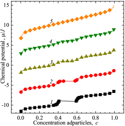
Figure 3: (Colour online) The chemical potential (in units of the interaction energy of the nearest neighbors $J$) versus concentration at $T/T_{c}=0.80$ (curves 1); 0.95 (2); 1.05 (3); 1.20 (4) and 2.00 (5). The solid lines represent the DA results, the full symbols are the MC simulation data. Each group of curves is shifted down by 5 units with respect to the previous one for better visibility. The unshifted curve 3 is characterized by $\mu/J=$ 1 at $c=0.5$, and this point is the same for all the temperatures. Thus, the groups of curves 1 and 2 are shifted down from their true position, while the groups 4 and 5 are shifted up.

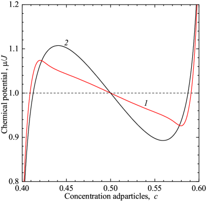
Figure 4: (Colour online) Chemical potential isotherms at $T/T_{c}=0.80$. Curve 1 represents the results of the quasi-chemical approximation, curve 2 — the diagram approximation.

Comparison of the results of analytical calculations and modelling showed that the parameter $\lambda$ included in relation (4.2), which ensures the equality of the critical parameters of the system found during its modelling and calculated within the framework of the diagram approximation, is equal to 1.10308. It can be noted that its value differs very insignificantly from the analogous value obtained for a system with attraction between nearest neighbors [33].

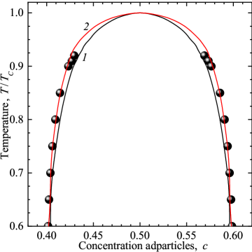
Figure 5: (Colour online) Phase diagram of the lattice fluid with the repulsion of nearest neighbors on a two-level lattice. Solid lines represent the results of the quasi-chemical (curve 1) and the diagram (curve 2) approximations. The full circles are the MC simulation results.

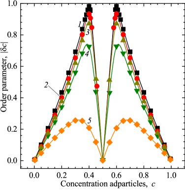
Figure 6: (Colour online) The order parameter versus concentration for $T/T_{c}=0.80$ (curves 1); 0.95 (2); 1.05 (3); 1.20 (4) and 2.00 (5). The solid lines represent the diagram approximation results, the full circles are the MC simulation data.

The isotherms of the chemical potential calculated for temperatures above and below the critical temperature $T_{c}$ are show in figure 3. Figure 4 shows the isotherms of the chemical potential at a temperature of $0.8T_{c}$ determined within the framework of the quasi-chemical and diagram approximation.

It can be seen from the comparison (figure 3) that the results of the diagram approximation are in good agreement with the results of MC simulation in the entire range of the considered temperatures and concentrations. As expected, in the two-phase region, the approximate approaches give a Van der Waals loop (see figure 4), while the simulation of the system demonstrates the constancy of the chemical potential. This allows us to conclude that a first-order phase transition is observed in the case of a two-level lattice.

Maxwell’s construction allows you to determine the points of phase transitions. The phase diagram of the system is shown in figure 5. The phase diagram turns out to be much narrower compared to the system with attractive interaction [33].

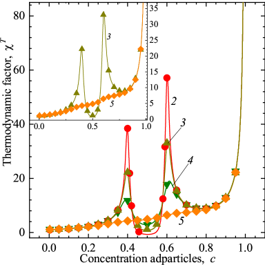
Figure 7: (Colour online) The thermodynamic factor versus concentration at $T/T_{c}=0.95$ (curves 2); 1.05 (3); 1.20 (4) and 2.00 (5). The solid line represents the DA results, the full circles are the MC simulation data.

Figure 8: (Colour online) The correlation functions for nearest neighbors versus concentration at $T/T_{c}=0.80$ (curves 1); 0.95 (2); 1.05 (3); 1.20 (4) and 2.00 (5). The solid lines represent the DA results, the full circles are the MC simulation data.

In general, it can be noted that the thermodynamic characteristics do not qualitatively reveal the new properties in comparison with a similar system with the attraction of the nearest neighbors.

By contrast, the structural properties — the order parameter (figure 6), the thermodynamic factor (figure 7) and the correlation function (figure 8) — show the new features qualitatively.

For example, the order parameter is much larger than for the fluid with attraction between particles [33], and decreases monotonously with increasing temperature. In this case, in contrast to the one-level system [22], the order parameter turns out to be nonzero even at temperatures above the critical one.

One can also see a sharp increase in the thermodynamic factor at particle concentrations near 0.4 and 0.6. This behavior of the thermodynamic factor is explained by the fact that at a sufficiently low temperature and at concentrations less than 0.4, deeper $\gamma$-sites are predominantly filled. At $c=0.4$, the $\gamma$-sublattice is almost filled, and the transition of the particle to the $\alpha$-sublattice is energetically unfavorable both because the $\alpha$-sites are shallower and because of the repulsion between the particles.

Thus, at a concentration of $c=0.4$, the mobility of particles sharply decreases. A similar situation is observed at a concentration of 0.6 with the only difference that, due to the interaction between particles at this concentration, the $\alpha$-sites are predominantly filled, and the $\gamma$ sublattice is almost completely empty.

The features in the dependence of the correlation functions on the concentration shown in figure 8 can be explained in a similar way. The sharp increase in the correlation function in the concentration range of 0.4 and 0.6 for temperatures close to the critical one is due to an equally sharp decrease in the concentration of particles on one of the sublattices.

6 Conclusion

Comparison of the results of the developed approximate methods and simulation data shows that these results are in full qualitative and quantitative agreement in the entire range of temperature and concentration variation. This makes it possible to use, for example, the diagram approximation to study the thermodynamic and structural characteristics of the lattice fluid on a two-level lattice, since DA does not require powerful computers as compared with MC method.

The proposed quasi-chemical approximation refinement method is not the only possible one. Another strategy can be implemented within the framework of the so-called self-consistent diagram approximation. The main idea of the latter is to consider a reference system in which the range of the average potentials exceeds the range of the interaction potentials [29]. However, this approach leads to a significant complication of the obtained relations, which complicates their subsequent analysis.

It can also be noted that in the case of the system with repulsive interaction, the transition from a one-level to a two-level system changes the kind of phase transition in it.

To explain this fact, the isotherm of the chemical potential at low temperature (see curve 1 in figure 3) must be considered together with the corresponding dependence of the order parameter versus concentration. The number of particles on the lattice increases monotonously with an increase in the chemical potential at low temperatures and low concentrations. In this case, as follows from figure 6 (see curve 1), deep $\gamma$-sites are predominantly filled. Obviously, such distribution of particles on the lattice is possible up to the concentration of 0.4. When this limit is reached, all $\gamma$-sites will be occupied and additional particles can be placed on shallow $\alpha$-sites. In this case, each particle on $\alpha$-sublattice will receive 2 nearest neighbors. Therefore, due to the interaction between particles, the concentration of particles increases with a jump to 0.6 when the chemical potential reaches a critical value. This corresponds to the situation when all the $\alpha$-sites are occupied, and the $\gamma$-sites are vacant. There is a plateau on the isotherm of the chemical potential which corresponds to the phase transitions of the first order.

Thus, the phase transition itself corresponds to the transition between two different ordered states of the system. In the first of them, the deep $\gamma$-sublattice is predominantly occupied, and in the second, the shallow $\alpha$-sublattice is predominantly occupied. This conclusion is fully confirmed by the analysis of snap-shots of the simulation procedure. An increase in temperature reduces the ordering of the system. However, this ordering is essential at a sufficiently high temperature $2T_{c}$ (see curve 5 in figure 6) and does not disappear even at extremely high temperatures ($10^{3}T_{c}$).

Ukrainian 0

[Ðiâíîâàæíi âëàñòèâîñòi äâîðiâíåâîãî ґðàòêîâîãî ôëþ¿äó]Ðiâíîâàæíi âëàñòèâîñòi ґðàòêîâîãî ôëþ¿äó íà äâîõðiâíåâié ґðàòöi ç íåïðÿìîêóòíîþ ãåîìåòðiєþ òà âiäøòîâõóâàííÿì ìiæ íàéáëèæчèìè ñóñiäàìè

[ß. Ã. Ãðîäà]ß. Ã. Ãðîäà

             
Áiëîðóñüêèé äåðæàâíèé òåõíîëîãiчíèé óíiâåðñèòåò, âóë. Ñâåðäëîâà 13a, 220006 Ìiíñüê, Áiëîðóñü

References

- [1] Domb C., Adv. Phys., 1960, 9, 149–361, doi:10.1080/00018736000101199.
- [2] Stromme M., Solid State Ionics, 2000, 131, 261–273, doi:10.1016/S0167-2738(00)00674-3.
-
[3]
Vakarin E. V., Holovko M. F., Chem. Phys. Lett., 2001, 349, 13–18,
doi:10.1016/S0009-2614(01)01185-X. -
[4]
Bisquert J., Vikhrenko V. S., Electrochim. Acta, 2002, 47, 3977–3988,
doi:10.1016/S0013-4686(02)00372-9. -
[5]
Levi M. D., Wang C., Aurbach D., Chvoj Z., J. Electroanal.
Chem., 562, 187–203,
doi:10.1016/j.jelechem.2003.08.032. -
[6]
Garcia-Belmonte G., Vikhrenko V., Garcia-Canadas J., Bisquert J.,
Solid State Ionics, 2004, 170,
123–127, doi:10.1016/j.ssi.2004.02.009. -
[7]
Groda Ya., Dudka M., Kornyshev A. A., Oshanin G., Kondrat S., J. Phys. Chem. C,
2021, 125,
4968–4976, doi:10.1021/acs.jpcc.0c10836. -
[8]
Vorotyntsev M. A., Badiali J. P., Electrochim. Acta, 1994, 39, 289–306,
doi:10.1016/0013-4686(94)80064-2. - [9] Chvoj Z., Conrad H., Chab V., Surf. Sci., 1997, 376, 205–218, doi:10.1016/S0039-6028(96)01290-3.
- [10] Chvoj Z., Conrad H., Chab V., Surf. Sci., 1999, 442, 455–462, doi:10.1016/S0039-6028(99)00960-7.
- [11] Masin M., Chvoj Z., Conrad H., Surf. Sci., 2000, 457, 185–198, doi:10.1016/S0039-6028(00)00353-8.
-
[12]
Tarasenko A. A., Chvoj Z., Jastrabik L., Nieto F., Uebing C., Phys. Rev. B, 2001,
63,
165423, doi:10.1103/PhysRevB.63.165423. -
[13]
Tarasenko A. A., Chvoj Z., Jastrabik L., Nieto F., Uebing C., Surf. Sci., 2001,
482–485,
396–401, doi:10.1016/S0039-6028(01)00799-3. -
[14]
Tarasenko A. A., Jastrabik L., Surf. Sci., 2002, 507–510, 108–113,
doi:10.1016/S0039-6028(02)01184-6. -
[15]
Nieto F., Tarasenko A. A., Uebing C., Appl. Surf. Sci., 2002, 196,
181–190,
doi:10.1016/S0169-4332(02)00054-5. -
[16]
Tarasenko A. A., Jastrabik L., Muller T., Surf. Sci., 2007, 601, 4001–4004,
doi:10.1016/j.susc.2007.04.030. - [17] Tarasenko A. A., Jastrabik L., Surf. Sci., 2008, 602, 2975–2982, doi:10.1016/j.susc.2008.07.037.
- [18] Tarasenko A. A., Jastrabik L., Physica A, 2009, 388, 2109–2121, doi:10.1016/j.physa.2009.02.009.
- [19] Tarasenko A. A., Jastrabik L., Appl. Surf. Sci., 2010, 256, 5137–5144, doi:10.1016/j.apsusc.2009.12.076.
- [20] Tarasenko A. A., Jastrabik L., Surf. Sci., 2015, 641, 266–268, doi:10.1016/j.susc.2015.02.008.
- [21] Tarasenko A. A., Bohac P., Jastrabik L., Physica E, 2015, 74, 556–560, doi:10.1016/j.physe.2015.08.027.
-
[22]
Vikhrenko V. S., Groda Ya. G., Bokun G. S. Equilibrium and diffusion characteristics of
the
intercalation systems on the basic of the lattice models, Minsk, Belarusian State Technological University, 2008,
URL https://elib.belstu.by/handle/123456789/2716 (in Russian). -
[23]
Groda Y. G., Lasovsky R. N., Vikhrenko V. S., Solid State Ionics, 2005, 176,
1675–1680,
doi:10.1016/j.ssi.2005.04.016. -
[24]
Metropolis N., Rosenbluth A. W., Rosenbluth M. N., Teller A. H.,
J. Chem. Phys., 1953, 21,
1087–1092, doi:10.1063/1.1699114. - [25] Uebing C., Gomer R. A., J. Chem. Phys., 1991, 95, 7626–7652, doi:10.1063/1.461817.
-
[26]
Groda Ya. G., Vikhrenko V. S., di Caprio D., Condens. Matter Phys., 2018,
21, 43002,
doi:10.5488/CMP.21.43002. -
[27]
Groda Ya. G., Vikhrenko V. S., di Caprio D., J. Belarus. State Univ. Physics, 2019, 2, 84–95,
doi:10.33581/2520-2243-2019-2-84-95 (in Russian.) -
[28]
Groda Ya. G., Grishina V. S., Ciach A., Vikhrenko V. S.,
J. Belarus. State Univ. Physics, 2019,
3, 81–91,
doi:10.33581/2520-2243-2019-3-81-91 (in Russian). -
[29]
Bokun G. S., Groda Ya. G., Belov V. V., Uebing C., Vikhrenko V. S., Eur. Phys. J. B,
2000, 15,
297–304, doi:10.1007/S100510051128. -
[30]
Vikhrenko V. S., Groda Ya. G., Bokun G. S., Phys. Lett. A, 2001,
286, 127–133,
doi:10.1016/S0375-9601(01)00408-X. -
[31]
Groda Ya. G., Argyrakis P., Bokun G. S., Vikhrenko V. S., Eur. Phys. J. B,
2003, 32, 527–535,
doi:10.1140/epjb/e2003-00118-3. -
[32]
Mayer J. E., Mayer M. G., Statistical Mechanics, John Wiley and Sons, New York, 2nd edn.,
1977, doi:10.1002/qua.560150209. - [33] Groda Ya. G., J. Belarus. State Univ. Physics, 2021 (submitted).
Ukrainian \adddialect\l@ukrainian0 \l@ukrainian