Tests of General Relativity with Gravitational-Wave Observations
using a Flexible–Theory-Independent Method

Abstract

We perform tests of General Relativity (GR) with gravitational waves (GWs) from the inspiral stage of compact binaries using a theory-independent framework, which adds generic phase corrections to each multipole of a GR waveform model in frequency domain. This method has been demonstrated on LIGO-Virgo observations to provide stringent constraints on post-Newtonian predictions of the inspiral and to assess systematic biases that may arise in such parameterized tests. Here, we detail the anatomy of our framework for aligned-spin waveform models. We explore the effects of higher modes in the underlying signal on tests of GR through analyses of two unequal-mass, simulated binary signals similar to GW190412 and GW190814. We show that the inclusion of higher modes improves both the precision and the accuracy of the measurement of the deviation parameters. Our testing framework also allows us to vary the underlying baseline GR waveform model and the frequency at which the non-GR inspiral corrections are tapered off. We find that to optimize the GR test of high-mass binaries, comprehensive studies would need to be done to determine the best choice of the tapering frequency as a function of the binary’s properties. We also carry out an analysis on the binary neutron-star event GW170817 to set bounds on the coupling constant $\alpha_{0}$ of Jordan-Fierz-Brans-Dicke gravity. We take two plausible approaches; the first approach involves translating directly the theory-agnostic bound on dipole-radiation into a bound on $\alpha_{0}$ for different neutron-star equations of state (EOS). The second theory-specific approach involves reparameterizing the test such that the deviation parameter is $\alpha_{0}$ itself. The two approaches provide slightly different bounds, namely, $\alpha_{0}\lesssim 2\times 10^{-1}$ and $\alpha_{0}\lesssim 4\times 10^{-1}$, respectively, at $68\%$ credible level. These differences arise mainly since in the theory-specific approach the tidal and scalar-charge parameters are fixed coherently for each neutron-star EOS and mass.

I Introduction

Over the past half-decade, observations of gravitational waves (GWs) have gone from being elusive to the routine. Since the first detection of GWs in September 2015 Abbott et al. (2016a), the LIGO Aasi et al. (2015) and Virgo Acernese et al. (2015) detectors have observed almost a hundred GW signals Abbott et al. (2021a) from mergers of black holes (BHs), neutron stars (NSs) Abbott et al. (2017a, 2020a) and their mixture Abbott et al. (2021b). Placed alongside independent confirmations of these detections, as well as, claims of new ones Nitz et al. (2019a, b); Venumadhav et al. (2020); Zackay et al. (2019); Nitz et al. (2021); Olsen et al. (2022), these results have firmly established the field of GW astronomy.

Besides attempting answers in astrophysics Abbott et al. (2017b, 2018a, 2021c) and cosmology Abbott et al. (2021d, e) in a manner complementary to electromagnetic astronomy, GWs are unique probes of fundamental physics. For more than a century, Albert Einstein’s theory of General Relativity (GR) has been our description of gravitational interactions, having passed every experimental and observational challenge, so far. However, for the first time, the LIGO-Virgo GW observations have allowed us to probe GR in the large-velocity, highly dynamical, strong-field regime of gravity, a regime which is inaccessible with tests in the Solar System Will (2014), in binary pulsars Wex (2014), and with observations around supermassive BHs at the center of galaxies Abuter et al. (2018); Do et al. (2019); Akiyama et al. (2019).

Tests of GR with GW observations come in two distinct flavors: theory agnostic and theory specific. The first class of tests assumes that the underlying GW signal is well-described by GR, and any potential deviation is characterized by extra, phenomenological, non-GR degrees of freedom or parameters. These tests use observations of GWs to constrain the non-GR parameters and check for consistency with their nominal predictions in GR. While theory-agnostic tests can only comment on (dis)agreement with GR predictions, the above measurements of phenomenological non-GR parameters can be translated to specific modified theories of gravity, albeit there are subtleties, as we shall discuss below. Investigations that compare directly the data with modified theories of gravity belong to the theory-specific flavor of tests of GR.

Several tests of GR have been demonstrated using the observations of GW signals by the LIGO-Virgo Collaboration (LVC) Abbott et al. (2016b, c, 2018b, 2019, 2021f, 2021g). Among them are the theory-agnostic parameterized tests of the inspiral, which check for the agreement of the early evolutionary (or inspiral) phase of a compact binary coalescence composed of BHs and/or NSs with the analytic post-Newtonian (PN) approximation for binaries in GR Arun et al. (2006); Yunes and Pretorius (2009); Mishra et al. (2010); Li et al. (2012); Agathos et al. (2014). Parameterized GR waveforms have used the LIGO-Virgo observations to provide state-of-the-art bounds on possible deviations from the PN predictions Abbott et al. (2021f). At the same time, these theory-agnostic bounds have been used to conduct theory-specific tests and constrain particular modified theories of gravity (see, e.g., Refs. Yunes et al. (2016); Nair et al. (2019); Sennett et al. (2020); Nair and Yunes (2020); Perkins et al. (2021a)).

And yet, parameterized inspiral tests are not all exactly the same; they can differ in the underlying GR waveform model, in how the non-GR parameters are introduced into it, and in the transition beyond the inspiral part. In this work, we develop a framework to examine how the details of the construction of parameterized waveform models systematically affect the tests of GR in which they are employed . It is also important to be able to distinguish deviations from GR due to systematic uncertainties of the waveform model from true violations of the theory. This infrastructure allows us to add generic corrections to the inspiral portion of any gravitational waveform, thereby allowing tests of GR with a broader range of waveform models than previously possible (e.g., with the TIGER infrastructure Li et al. (2012); Agathos et al. (2014)). We call this framework the flexible theory-independent (FTI) approach, and explore it using synthetic binary BH (BBH) GW signals. In addition, the conveniently adaptable design of the FTI framework allows us for easy construction of waveform models for theory-specific tests. As an example, we apply the FTI framework to the first binary NS (BNS) merger observed by the LIGO and Virgo detectors, GW170817, and set bounds on the Jordan-Fierz-Brans-Dicke (JFBD) scalar-tensor theory of gravity. We note that the FTI approach has already been extensively used by LIGO and Virgo data analysts in Refs. Abbott et al. (2018b, 2019, 2021f, 2021g) and also by some of the authors of this manuscript in Ref. Sennett et al. (2020).

This paper is organized as follows. In Sec. II we introduce the FTI method for multipolar waveform models of compact-object binaries. After recalling the tenets of Bayesian inference in Sec. III, in Sec. IV we apply the FTI method to synthetic GW signals of BBHs. This allows us to discuss the effect of the FTI parameterization on the recovery of the BBH properties (excluding the GR-deviation parameters) and to study the robustness of the FTI method. In Sec. V, we use the FTI construction on real data, notably the BNS signal GW170817, to set bounds on the JFBD theory of gravity. Finally, in Sec. VI, we summarize our main conclusions and also discuss possible future work. The Appendix A collects the necessary PN results for the GW phase of BBH with aligned spins.

Henceforth, we use natural units such that the Newton constant $G=1$ and the speed of light $c=1$.

II The FTI approach

In GR, gravitational signals from quasi-circular BBHs depend on the instrinsic parameters $\bm{\lambda}=\{m_{1},m_{2},\bm{S}_{1},\bm{S}_{2}\}$, where $m_{i},\bm{S}_{i}$ are the masses and spins of the compact objects ($i=1,2$), as well as, a set of extrinsic parameters $\bm{\xi}=\{\iota,\varphi_{c},\alpha,\delta,\psi,d_{L},t_{c}\}$. These are the angular position of the line of sight measured in the source frame ($\iota$, $\varphi_{c}$), the sky location of the source in the detector frame $(\alpha,\delta)$, the polarization angle $\psi$, the luminosity distance of the source $d_{L}$ and the time of arrival $t_{c}$. Limiting ourselves to objects with non-precessing spins (i.e., spins aligned or antialigned with the orbital angular momentum ${\bm{L}}$), the only (dimensionless) spin component on which the dynamics, and hence the waveform, depends is $\chi_{i}=\bm{S}_{i}\cdot{\bm{L}}/(|\bm{L}|m_{i}^{2})$. The set of instrinsic parameters consequently reduces to four $\bm{\lambda}=\{m_{1},m_{2},\chi_{1},\chi_{2}\}$. For convenience, we additionally introduce the following parameters: the mass ratio $q=m_{1}/m_{2}\geq 1$, the symmetric mass ratio $\nu=q/(1+q)^{2}$, the binary’s total mass $M=m_{1}+m_{2}$, the chirp mass ${\cal M}=\nu^{3/5}\,M$, and the effective spin $\chi_{\rm{eff}}=(m_{1}\chi_{1}+m_{2}\chi_{2})/M$. The above set of 11 parameters is enough to describe an aligned-spin BBH signal. For a binary involving NSs, this set increases by the tidal parameters ($\Lambda_{1,2}$), which encode the NS matter equation of state.

In GR, the GW signal can be decomposed into a set of modes by projecting the complex linear combination of its plus and cross polarizations

$$h(t)\equiv h_{+}(t)-ih_{\times}(t)\,,$$ (1)

onto spherical harmonics ${}_{-2}Y_{\ell m}$ of spin-weight $-2$ Pan et al. (2011),

$$h(t;\bm{\lambda},\iota,\varphi_{c})=\sum^{+\infty}_{\ell=2}\sum_{m=-\ell}^{\ell}{}_{-2}Y_{\ell m}(\iota,\varphi_{c})\,h_{\ell m}(t,\bm{\lambda})\,.$$ (2)

During the inspiral, the GW signals from aligned-spin binaries satisfy a reflection symmetry about its orbital plane, which implies

$$h_{\ell-m}(t)=(-1)^{\ell}h_{\ell m}^{*}(t)\,.$$ (3)

where ^∗ denotes the complex conjugation. As a consequence, we can restrict ourselves to the $m\geq 0$ modes to describe the complete mode-content of aligned-spin inspiral waveforms. Furthermore, for such systems, $\tilde{h}^{R}_{\ell m}(f)$, the Fourier transform of the real part of $h_{\ell m}(t)$ is related to the imaginary part via

$$\tilde{h}^{R}_{\ell m}(f)=-i\tilde{h}^{I}_{\ell m}(f)\,.$$ (4)

Using Eq. (3) and  (4), the GW polarizations in the frequency domain read (see Appendix C of Ref. Mehta et al. (2017) for full derivation)

$${\tilde{h}}_{+}(f) =\sum^{+\infty}_{\ell=2}\sum_{m=1}^{\ell}\,\Bigr{[}(-1)^{\ell}f(\iota)+1\Bigr{]}\,{}_{-2}Y_{\ell m}(\iota,\varphi_{c})\,\tilde{h}^{R}_{\ell m}(f)\,,$$ (5a)

$${\tilde{h}}_{\times}(f) =-i\sum^{+\infty}_{\ell=2}\sum_{m=1}^{\ell}\,\Bigr{[}(-1)^{\ell}f(\iota)-1\Bigr{]}\,{}_{-2}Y_{\ell m}(\iota,\varphi_{c})\,\tilde{h}^{R}_{\ell m}(f)\,,$$ (5b)

with

$$f(\iota)=\frac{d_{\,\ell-m}^{\,2}(\iota)}{d_{\,\ell m}^{\,2}(\iota)}\,,$$

where $d_{\,\ell m}^{\,2}(\iota)$ denote the Wigner functions of weight $-2$ Wiaux et al. (2007). Being a complex function, $\tilde{h}^{R}_{\ell m}(f)$ can be written as

$$\tilde{h}^{R}_{\ell m}(f)=A_{\ell m}(f)\,e^{i\,\psi_{\ell m}(f)}.$$ (6)

The construction of a parameterized (or generalized) waveform model begins with the baseline model in GR (Eq. (6)). During the quasi-circular, adiabatic inspiral, the frequency-domain phase $\psi_{\ell m}(f)$ can be obtained from PN theory Blanchet (2014); Buonanno et al. (2009) using the stationary-phase approximation (SPA). In GR it reads

$$\psi_{\ell m}^{\text{(GR)}}(f,\bm{\lambda})= \frac{3}{128\nu v^{5}}\frac{m}{2}\left[\sum_{n=0}^{7}\psi_{n}^{\text{(PN)}}(\bm{\lambda})v^{n}+\right.$$

$$\left.\sum_{n=5}^{6}\psi_{n(l)}^{\text{(PN)}}(\bm{\lambda})v^{n}\log v\right],$$ (7)

where

$$v\equiv\left(2\pi FM\right)^{1/3}=\left(2\pi fM/m\right)^{1/3}.$$ (8)

The quantity $F$ is the orbital frequency which is related to the (Fourier) GW frequency $f$ for a given $(\ell,m)$-mode through the equation above. The quantities $\psi_{n}^{\text{(PN)}}$ and $\psi_{n(l)}^{\text{(PN)}}$ are the $(n/2)$-PN coefficients . which depend on the binary parameters. In the Appendix A, we provide explicit expressions for the PN coefficients up to 3.5PN order (including spin effects), the highest PN order to which the GW phasing is currently known. Note that the logarithmic terms in Eq. (7) arise from tails effects (i.e., terms that depend on the complete past history of the binary).

We generalize the GR waveform model by considering corrections to the phase that take a form similar to the PN expansion

$$\delta\psi_{\ell m}(f,\bm{\lambda};\delta\hat{\varphi}_{n},\delta\hat{\varphi}_{n(l)}) =\frac{3}{128\nu v^{5}}\frac{m}{2}\left[\sum_{n=-2}^{7}\delta\psi_{n}(\bm{\lambda},\delta\hat{\varphi}_{n})v^{n}\right.$$

$$\left.+\sum_{n=5}^{6}\delta\psi_{n(l)}(\bm{\lambda},\delta\hat{\varphi}_{n(l)})v^{n}\log v\right],$$ (9)

where $\delta\psi_{n}$ and $\delta\psi_{n(l)}$ are deviations to the $(n/2)$-PN phase coefficients $\psi_{n}^{\text{(PN)}}$ and $\psi_{n(l)}^{\text{(PN)}}$ defined above. These correction terms depend, in addition to $\bm{\lambda}$, also on the corresponding deviation parameter $\delta\hat{\varphi}_{n}$ or $\delta\hat{\varphi}_{n(l)}$, respectively. We include possible deviations at “pre-Newtonian” orders ($n<0$) as these are predicted in some alternative theories of gravity. In particular the emission of dipole radiation (discussed in Sec. V.1) leads to a nonvanishing deviation at $n=-2$. A solitary deviation at $n=-1$ is less well motivated and not discussed in this work. Parameterized deviations of this form can be mapped onto the predictions of any hypothetical theory of gravity provided that (i) the theory admits a weak-field, slow-velocity PN expansion as in GR, and (ii) the deviations from GR are parametrically smaller than the PN-expansion parameter $v^{2}$. Note that this excludes theories that admit non-perturbative phenomena like dynamical scalarization, for which the naive PN expansion in Eq. (9) breaks down Palenzuela et al. (2014); Sennett and Buonanno (2016), and other methods are needed to observe such effects (see, e.g., Ref. Edelman et al. (2021)). Because GW detectors are more sensitive to the evolution of the signal’s phase than its amplitude, considering also the computational cost of introducing several free parameters, we neglect deviations in the mode amplitudes $A_{\ell m}$.

Despite the generality of Eq. (9), the moderate signal-to-noise ratios (SNRs) of most LIGO-Virgo observations, so far, do not allow us to place meaningful bounds on multiple deviation parameters concurrently. Hence, we vary one parameter at a time, keeping the rest fixed at their nominal GR prediction, which is zero. This assumption is validated by investigations Sampson et al. (2013); Meidam et al. (2018); Perkins et al. (2021a); Perkins and Yunes (2022) that conclude that a signal containing deviations at several PN orders is likely to lead to a non-zero deviation measurement using a model with only a single deviation parameter. On the other hand, a recent work Saleem et al. (2021) following a principle component analysis identified certain combinations of these deviation parameters with the tightest constraints; in fact, the two dominant principle components rather capture the essence of the full multi-parameter test.

In this paper, we assume that each deviation parameter represents a fractional deviation to the corresponding PN coefficient in GR and for this reason, we also refer to the deviation parameters as non-GR parameters,

$$\delta\psi_{n}(\bm{\lambda},\delta\hat{\varphi}_{n}) \equiv\delta\hat{\varphi}_{n}\psi_{n}^{(\text{PN})}(\bm{\lambda}),$$ (10a)

$$\delta\psi_{n(l)}(\bm{\lambda},\delta\hat{\varphi}_{n(l)}) \equiv\delta\hat{\varphi}_{n(l)}\psi_{n(l)}^{(\text{PN})}(\bm{\lambda}).$$ (10b)

We handle PN orders for which GR coefficients vanish slightly differently (i.e., for $n=-2$, $-1$, $1$). For such cases, we let $\varphi_{n}$ represent an absolute deviation at that order instead.

While Eq. (9) unambiguously details how to generalize GR waveforms containing only the inspiral, additional care must be taken for waveforms that contain later portions of the GW signal, such as the merger-ringdown. For the FTI approach, we require that the parameterized deviations satisfy the following properties

1. The early-inspiral (low-frequency) waveform has a phase $\psi_{\ell m}(f;\bm{\lambda};\delta\hat{\varphi}_{n},\delta\hat{\varphi}_{n(l)})=\psi_{\ell m}^{\text{(GR)}}(f;\bm{\lambda})+\delta\psi_{\ell m}(f;\bm{\lambda};\delta\hat{\varphi}_{n},\delta\hat{\varphi}_{n(l)})$, where $\delta\psi_{\ell m}$ takes the form of Eq. (9).

2. The post-inspiral (high-frequency) waveform has a phase $\psi_{\ell m}(f;\bm{\lambda};\delta\hat{\varphi}_{n},\delta\hat{\varphi}_{n(l)})=\psi_{\ell m}^{(\text{GR})}(f;\bm{\lambda})$ that exactly reproduces the underlying GR polarizations (Eq. (5)) up to some constant shift which represents the total dephasing from the GR polarization accumulated over the inspiral.

3. The waveform polarizations are $C^{2}$ smooth over all frequencies.

Using Eq. (10), the $\delta\psi_{\ell m}(f;\bm{\lambda};\delta\hat{\varphi}_{n},\delta\hat{\varphi}_{n(l)})$ in Eq. (9) read

$$\delta\psi_{\ell m}(f,\bm{\lambda};\delta\hat{\varphi}_{n},\delta\hat{\varphi}_{n(l)})\equiv \frac{3}{128\nu v^{5}}\frac{m}{2}\left[\sum_{n=-2}^{7}\psi_{n}^{\text{(PN)}}(\bm{\lambda})\delta\hat{\varphi}_{n}v^{n}\right.$$

$$\left.+\sum_{n=5}^{6}\psi_{n(l)}^{\text{(PN)}}(\bm{\lambda})\delta\hat{\varphi}_{n(l)}v^{n}\log v\right].$$ (11)

To smoothly apply these corrections over only the inspiral, we use a tapering function $W(f;v^{\text{tape}},\Delta v^{\text{tape}})$ given by

$$W(f;v^{\text{tape}},\Delta{v}^{\text{tape}})\equiv\left[1+\exp\left(\frac{v-v^{\text{tape}}}{\Delta v^{\text{tape}}}\right)\right]^{-1},$$ (12)

which smoothly transitions between one and zero around $v^{\text{tape}}$ over the range of $\sim\Delta v^{\text{tape}}$, where $v$ is defined in Eq. (8). We construct the total phase correction for a given $(\ell,m)$-mode by combining this windowing function with the second derivative with respect to frequency of $\delta\psi_{\ell m}$, which we denote as $\psi_{\ell m}^{\prime\prime}(f^{\prime\prime})$, and re-integrating with appropriate integration constants to ensure $C^{2}$ smoothness. In summary, we use

$$\delta\psi_{\ell m}(f;\bm{\lambda};\delta\hat{\varphi}_{n},\delta\hat{\varphi}_{n(l)};v^{\text{tape}},\Delta{v}^{\text{tape}})=$$

$$\;\;\int_{f_{\ell m}^{\text{ref}}}^{f}df^{\prime}\int_{f_{22}^{\text{peak}}}^{f^{\prime}}df^{\prime\prime}\delta\psi_{\ell m}^{\prime\prime}(f^{\prime\prime},\bm{\lambda};\delta\hat{\varphi}_{n},\delta\hat{\varphi}_{n(l)})$$

$$\;\;\times W(f^{\prime\prime};v^{\text{tape}},\Delta{v}^{\text{tape}}),$$ (13)

where $f_{\ell m}^{\text{ref}}$ $(\equiv mf_{22}^{\text{ref}}/2)$ is the reference frequency at which the phase of the ($\ell m$)-mode vanishes. This choice ensures that the definition of the reference frequency does not change when we add these corrections to the GR waveform. The second integration boundary is fixed by requiring that the first derivative of $\delta\psi_{\ell m}(f)$ goes to zero at the frequency of the $(2,2)$-mode’s peak $f_{22}^{\text{peak}}$ (see Eq. (A8) of Ref. Bohé et al. (2017)). This requirement ensures that the alignment between the GR waveform and the modified GR waveform in the time-domain remains the same.

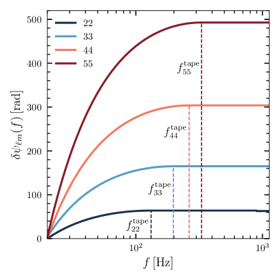
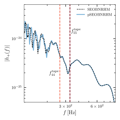
Figure 1: Left panel: The phase corrections for the different frequency-domain modes for the parameters of a GW190814-like event Abbott et al. (2020b) (see Table 1). The numerical value of the $(2,1)$-mode is relatively small and hence it is not shown in the plot for the sake of clarity. We use as tapering frequency $f^{\text{tape}}_{22}=0.35f_{22}^{\mathrm{peak}}$. The vertical dashed lines denote the tapering frequencies $f^{\text{tape}}_{\ell m}$ for each mode. The phase correction for each mode becomes constant for $f>f^{\text{tape}}_{\ell m}$ where they are tapered off. Right panel: The amplitude of the plus polarization of the SEOBNRHM and pSEOBNRHM waveforms. The amplitude of the pSEOBNRHM waveform returns to the GR (SEOBNRHM) one in the post-inspiral regime ($f>f^{\rm{tape}}_{44}$).

Let us elaborate more on the tapering parameters $v^{\rm{tape}}$ and $\Delta{v}^{\text{tape}}$ that enter the final expression for the phase corrections (13). Using Eq. (8), the parameter $v^{\rm{tape}}$ can be equivalently specified by the orbital frequency $F^{\mathrm{tape}}$ at which the corrections are tapered off. Note that while the orbital tapering frequency $F^{\text{tape}}$ is the same for all modes, the tapering frequency in Fourier domain $f^{\text{tape}}_{\ell m}=mF^{\text{tape}}$ depends on the mode. In the following, we fix the tapering frequency by specifying $f^{\text{tape}}_{22}$ as a fraction of $f_{22}^{\rm{peak}}$, say $f^{\text{tape}}_{22}=\alpha f_{22}^{\rm{peak}}$ with a constant $\alpha$ of order unity, and $v^{\text{tape}}=(\pi f_{22}^{\rm{tape}}M)^{1/3}$. Furthermore, instead of specifying the parameter $\Delta{v}^{\text{tape}}$ directly, we find it more useful to fix the number of GW cycles over which the window function defined in Eq. (12) switches its value from 0 to 1. The number of GW cycles $\mathcal{N}_{\rm GW}$ between the GW frequencies $f_{1}$ and $f_{2}$, or respectively $v_{1}$ and $v_{2}$ defined by Eq. (8), can be estimated as

$$\mathcal{N}_{\rm GW}=\int_{f_{1}}^{f_{2}}f(t)dt=\int_{f_{1}}^{f_{2}}df\dfrac{f}{\dot{f}}=\dfrac{1}{32\pi\nu}(v_{1}^{-5}-v_{2}^{-5}),$$ (14)

where we make use of the leading-order PN expressions for $f(t)$ and $\dot{f}(t)$ in the last equality. Now, choosing $v_{1,2}=v^{\mathrm{tape}}\mp\Delta v^{\mathrm{tape}}/2$, we solve for the small $\Delta{v}^{\text{tape}}\ll v^{\text{tape}}$,

$$\Delta{v}^{\text{tape}}=\frac{128\nu}{3}\pi(v^{\rm{tape}})^{6}\,\Gamma\,\mathcal{N}_{\rm GW}.$$ (15)

with the estimate $\Gamma\equiv\Gamma_{\text{PN}}=3/20$ from PN theory. However, since we are going to apply the tapering close to the merger of the binary, where the PN approximation is not applicable, we treat $\Gamma$ as a phenomenological fudge factor and choose $\Gamma=1/50$. The crucial input from PN theory is the functional dependence of $\Delta{v}^{\text{tape}}$ on $\nu$, $v^{\rm{tape}}$ and $\mathcal{N}_{\rm GW}$. The choice of the parameters $f^{\text{tape}}_{22}$ and $\mathcal{N}_{\rm GW}$ is completely phenomenological, and should be made to optimize the null test. Previous analyses on the LIGO-Virgo events reported in Refs. Abbott et al. (2021f, 2020c, 2020b, g) used $f^{\text{tape}}_{22}=0.35f_{22}^{\rm{peak}}$ and $\mathcal{N}_{\rm GW}=1$. While we also employ these choices for the studies here, we devote Sec. IV.2 to investigate how results are effected when varying, in particular, the tapering frequency $f^{\text{tape}}_{22}$. Changing $\mathcal{N}_{\rm GW}$ in the range $0.8\mbox{--}3$, instead, does not affect the results significantly.

At low frequencies, any GR description of the modes of the GW-phase reduces to the one of Eq. (7). Thus, we can apply the method outlined above to inspiraling PN models and also to inspiral-merger-ringdown GR models (if they are available in time domain we first perform a Fourier transform). Our method can treat the deviation coefficients in Eqs. (9) and (10) either as free parameters (see Sec. IV) or identify them to the ones predicted in specific alternative theories of gravity (see Sec. V), provided the latter have perturbative deviations from GR and are represented by PN-like coefficients. This is the eponymous flexibility of the FTI approach.

In this work, we apply the FTI approach to the multipolar, aligned-spin effective-one-body (EOB) waveform model SEOBNRHM Bohé et al. (2017); Cotesta et al. (2020) for BBHs, the aligned-spin EOB model SEOBNRT Bohé et al. (2017); Hinderer et al. (2016); Lackey et al. (2019) for BNSs, and for some studies, the aligned-spin inspiral-merger-ringdown phenomenological model PhenomX for BBHs Pratten et al. (2020) . The SEOBNR, SEOBNRT and PhenomX waveforms contain the $(\ell,m)=(2,2)$ (dominant) mode, while the SEOBNRHM waveforms include four additional sub-dominant modes, $(\ell,m)=(2,1)$, $(3,3)$, $(4,4)$, and $(5,5)$. We denote the waveforms to which we apply the non-GR phase corrections (10) parameterized waveforms and refer to them as pSEOBNRHM, pSEOBNRT and pPhenomX.

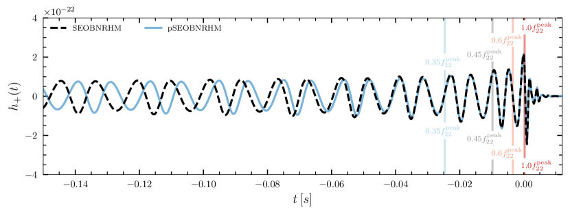
Figure 2: Plus polarization of the GR (SEOBNRHM) and pSEOBNRHM waveforms shown in Fig. 1. The waveforms are aligned at their peaks, $t=0$. The solid vertical lines denote the times corresponding to the different tapering frequencies that we employ in Sec. IV.2. Here, we use as tapering frequency in the pSEOBNRHM waveform $f^{\text{tape}}_{22}=0.35f_{22}^{\mathrm{peak}}$. The SEOBNRHM and the pSEOBNRHM waveforms match very well in the post-tapering region (i.e., for $t\geq t^{\rm{tape}}$ where $2F(t^{\rm{tape}})=0.35f_{22}^{\mathrm{peak}}$).

We end this section with an illustration of the tapering using the pSEOBNRHM model. We choose a binary with parameters that correspond to the median of the GW190814 Abbott et al. (2020b) event, as listed in Table 1, and generate two pSEOBNRHM waveforms corresponding to a deviation parameter of $\delta\hat{\varphi}_{2}=0.5$ and its GR limit $\delta\hat{\varphi}_{2}=0$ (i.e., identical to SEOBNRHM). Figure 1 shows contributions of the phase corrections $\delta\psi_{\ell m}^{\text{(PN)}}(f)$ to the different ($\ell,m$)-modes (left panel), as well as the amplitude of the plus polarizations after combining all the modes (via Eq. (5a)) for the SEOBNRHM and pSEOBNRHM waveforms (right panel). The vertical dashed lines mark the tapering frequency $f^{\text{tape}}_{\ell m}$ associated with the different modes. The left panel highlights how the correction to the phase for each mode, $\delta\psi_{\ell m}(f)$, approaches a constant value for $f>f^{\text{tape}}_{\ell m}$ where the correction is tapered off. Consistent with this, the right panel shows how the amplitude of the parameterized waveform (pSEOBNRHM) returns to the GR limit (SEOBNRHM) for $f>f_{44}^{\rm{tape}}$  We note that the parameterized waveform returns to the GR one when the overall phase difference, as illustrated in the left panel, becomes constant and is hence absorbed into the coalescence phase. In other words, the coalescence phase recovered using the parameterized waveforms and GR waveforms from the parameter-estimation studies is, in general, not expected to agree. In Fig. 2, we show the plus polarization of the parameterized and GR waveforms in time domain. The time-domain waveforms are generated from their frequency-domain counterparts via inverse Fourier transformation. The waveforms are aligned at the peak of their amplitudes. The vertical lines indicate the times corresponding to the tapering frequencies (i.e., $F(t^{\rm{tape}})\equiv F^{\rm{tape}}$), where the quantity $2F(t)$ is computed from the first derivative of the (2,2)-mode’s phase. For this figure, the tapering frequency used is $f^{\text{tape}}_{22}=0.35f_{22}^{\rm{tape}}=2F^{\rm{tape}}$, as stated before. For later analyses, we also indicate in the figure other choices of the tapering frequency. In the time-domain plot, it is visually clearer to see that the pSEOBNRHM waveform reduces to SEOBNRHM post-tapering (i.e., for $t\geq t^{\rm{tape}}$), while displaying a significant mismatch before the tapering (in the inspiral regime).

III Bayesian Inference

We can now use the parameterized waveforms introduced under the FTI approach in the previous section to perform tests of GR with LIGO-Virgo observations. The first step involves the measurement or inference of the waveform parameters, given the observed GW data. For this, we use a Bayesian approach in this paper. Given the hypothesis $\mathcal{H}$ that our data $d=h(\bm{\theta})+n$ consists of detector noise $n$ and a single GW signal, which can be accurately described by our waveforms $h(\bm{\theta})$ depending on parameters $\bm{\theta}=\{\bm{\lambda},\bm{\xi},\delta\hat{\varphi}_{n},\delta\hat{\varphi}_{n(l)}\}$, the Bayes’ theorem states that

$$P(\bm{\theta}|d,\mathcal{H})=\dfrac{\mathcal{L}(d|\bm{\theta},\mathcal{H})p(\bm{\theta}|\mathcal{H})}{E(d|\mathcal{H})}.$$ (16)

Here, $P(\bm{\theta}|d,\mathcal{H})$ is the posterior probability distribution of the parameters $\bm{\theta}$, and $p(\bm{\theta}|\mathcal{H})$ is the prior probability distribution. The quantity $E(d|\mathcal{H})$ is called the evidence of the hypothesis $\mathcal{H}$, which is just the normalization constant of the posterior probability distribution $P(\bm{\theta}|d,\mathcal{H})$. The quantity $\mathcal{L}(d|\bm{\theta},\mathcal{H})$ denotes the likelihood of obtaining the data $d=h(\bm{\theta})+n$ given that the parameters of the waveform are $\bm{\theta}$ under the hypothesis $\mathcal{H}$, the latter entailing the waveform and noise models. It is computed using

$$\mathcal{L}(d|\bm{\theta},\mathcal{H})\propto\exp\left[-\dfrac{1}{2}\langle d-h(\bm{\theta})|d-h(\bm{\theta})\rangle\right],$$ (17)

where $\langle.|.\rangle$ is the noise-weighted inner product,

$$\langle a|b\rangle=2\int_{f_{\rm{low}}}^{f_{\rm{high}}}\dfrac{\tilde{a}^{*}(f)\tilde{b}(f)+\tilde{a}(f)\tilde{b}^{*}(f)}{S_{n}(f)}df\,.$$ (18)

Equation (17) simply encodes our hypothesis of a stationary Gaussian noise model, with the power spectral-density (PSD) of the GW detector noise denoted by $S_{n}(f)$. We work with the three-detector network consisting of the two LIGO and the Virgo detectors. The quantities $f_{\rm{high}}$ and $f_{\rm{low}}$ denote the maximum and minimum frequencies, respectively, that enter in the likelihood estimation. The precise values of these quantities are dictated by the sensitivity bandwidth of the GW detectors. We will state them explicitly wherever required.

The prior probability distributions chosen for our analyses in this paper are identical to Ref. Veitch et al. (2015). More specifically, they are uniform in the component masses, isotropic in spin orientations and uniform in their magnitudes between $[0,0.99]$, uniform in the Euclidean volume for the luminosity distance, and isotropic in the sky location and binary orientation. We also choose a flat prior on our non-GR parmeters, $\delta\hat{\varphi}_{n}$, $\delta\hat{\varphi}_{n(l)}$. For the GW170817 analysis in Sec. V, we will introduce additional parameters and their priors below. With these prior distributions, we proceed to stochastically sample the parameter space using a Markov-Chain Monte Carlo (MCMC) algorithm provided in the $\tt{LALINFERENCE}$ code Veitch et al. (2015). The one-dimensional posterior distribution of a specific parameter (demonstrated, e.g., in Fig. 3) is then computed by simply marginalizing $P(\bm{\theta}|d,\mathcal{H})$ over the nuisance parameters.

We now utilize the Bayesian parameter inference outlined above to demonstrate the FTI approach in two specific cases: in the context of a theory-agnostic test with the BBH GW signals GW190412 and GW190814 (Sec. IV), and a theory-specific test with the BNS signal GW170817 (Sec. V).

IV Application of the FTI approach to binary black holes

The first of our two goals in this paper is to show the pliability of the FTI approach in performing theory-agnositc tests of GR, where one checks for the (dis)agreement between estimates of non-GR parameters with their GR predictions. In this section, we stress-test the FTI approach on GW signals, and explore its robustness against different assumptions made by different families of waveforms. We also investigate possible systematic biases when the underlying waveform model contains missing physics, for example, an absence of information due to higher modes (HMs). Finally, we scrutinize how “flexible” the FTI approach really is in its choice of internal settings like the tapering frequency. An incomplete model or an incorrect internal setting can potentially flag a violation of GR, and needs to be accounted for while performing theory-agnositc tests of GR.

These investigations also illuminate the robustness of parameterized theory-agnostic inspiral tests in general, which is more straightforward in an approach like FTI that strives to expose all flexibility (or arbitrariness) of the test. Comparing this to the TIGER infrastructure Li et al. (2012); Agathos et al. (2014), we note that TIGER is designed and implemented within a particular family of waveform models, with a specific prescription for the transition to the merger-ringdown phase being essentially inherited from the underlying GR waveform.

IV.1 FTI results with synthetic signals: GW190412-like and GW190814-like

Table 1: Median values and symmetric 90% credible intervals for the source-frame parameters of the GW190814 Abbott et al. (2020b) and GW190412 Abbott et al. (2020c) signals observed by LIGO and Virgo. We indicate the source-frame masses with the superscript $s$, to distinguish them from the detector-frame masses, $m_{i}=(1+z)\,m_{i}^{s}$, used in the rest of the paper. We use the median values for our synthetic signals: GW190814–like and GW190412–like signals.

Parameter	GW190814	GW190412
$m^{s}_{1}/M_{\odot}$	$23.2_{-1.0}^{+1.1}$	$30.1_{-5.3}^{+4.6}$
$m^{s}_{2}/M_{\odot}$	$2.59^{+0.08}_{-0.09}$	$8.3_{-0.9}^{+1.6}$
$1/q$	$0.112_{-0.009}^{+0.008}$	$0.28_{-0.07}^{+0.12}$
$\iota$ (rad)	$0.8_{-0.2}^{+0.3}$	$0.71_{-0.24}^{+0.31}$
$z$	$0.053_{-0.010}^{+0.009}$	$0.15_{-0.03}^{+0.03}$
$\rm{SNR}$	$25.0_{-0.2}^{+0.1}$	$19.1_{-0.3}^{+0.1}$

In this section, we explore the effect on theory-agnostic tests of varying the physical content in our waveform model, for instance, the impact of HMs. We restrict ourselves to GW signals from BBH mergers, specifically, the high-mass ratio GW190412 and GW190814 BBH signals, which show non-negligible evidence for the presence of HMs Abbott et al. (2020c, b). We note that the FTI analysis with HMs has been already performed by the LVC on these two events in Ref. Abbott et al. (2021f) (see Appendix C therein). Let us recapitulate those results here, summarized by the unfilled black histograms in Fig. 3. However, note that in LVC publications, the FTI results are typically transformed and reweighed to match the normalization of the TIGER inspiral parameters. This permits comparisons between the two approaches, generally finding good agreement for the GR constraints (see also Sec. V of Ref. Abbott et al. (2021f) for details). Throughout this work, we present the FTI results without such reweighing.

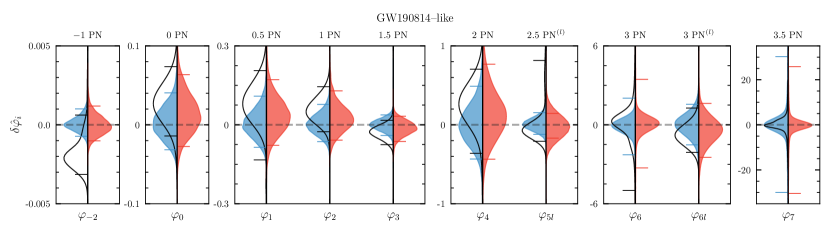
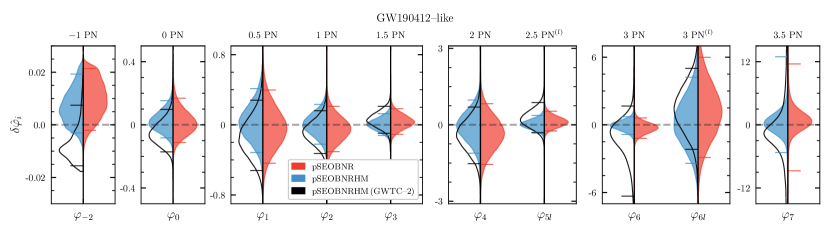
Figure 3: Filled histograms for the posterior distributions of the deviation parameters $\delta\hat{\varphi}_{i}$, $\delta\hat{\varphi}_{i(l)}$ appearing in Eq. (11) when a GR simulated signal using the pSEOBNRHM  waveform is analyzed with the parameterized waveforms pSEOBNRHM  (blue) and pSEOBNR  (orange) (top panel: GW190814–like parameters; bottom panel: GW190412-like parameters). The inclusion of HMs improves both the precision and the accuracy of the measurement of the deviation parameters. Also shown by the black unfilled histograms are the results obtained from the actual GW190814 and GW190412 events when analyzed with the pSEOBNRHM , as first presented in Ref. Abbott et al. (2021f) (but here without reweighing against the priors). The small symmetrical horizontal lines in each panel represent the 90% credible intervals.

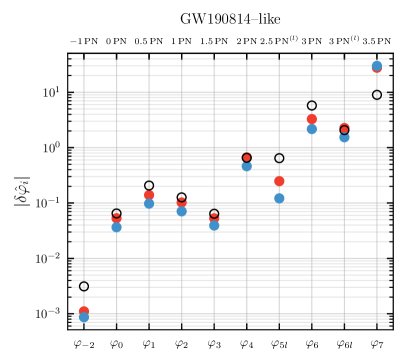
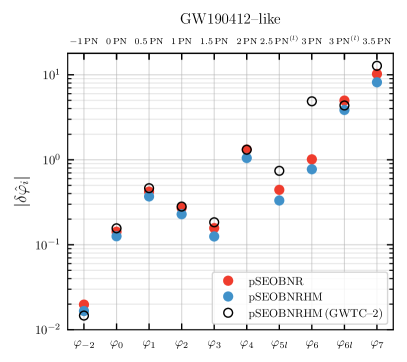
Figure 4: The 90% credible intervals of the posterior distributions of the deviation parameters in Fig. 3 (i.e., for the simulated GW190814–like (left panel) and GW190412–like (right panel) signals.) The HM waveforms, pSEOBNRHM , provide slightly better bounds. The open circles are the results from the actual events GW190814 and GW190412 Abbott et al. (2021f) (but here without reweighing against the priors).

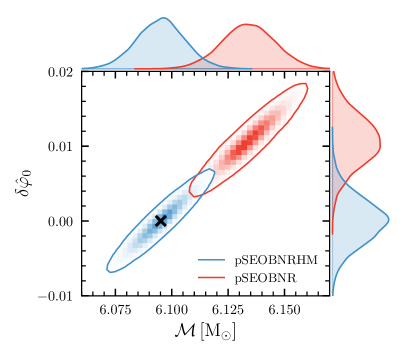
Figure 5: The same analysis as in Fig. 3 ($\mathrm{SNR}=25$) for the deviation parameter $\delta\hat{\varphi}_{0}$ with the GW190814–like signal but at the $\mathrm{SNR}=200$. The GR value (marked with a cross sign) with the $(2,2)$-mode waveform pSEOBNR  lies outside the 90% credible level indicating a deviation from GR.

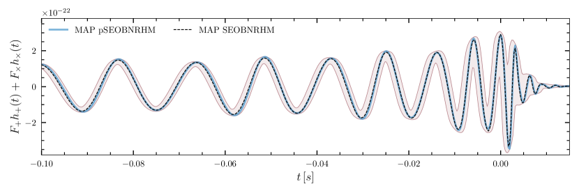
Figure 6: The detector-strain outputs $F_{+}\,h_{+}(t)+F_{\times}\,h_{\times}(t)$ (where $F_{+},F_{\times}$ are the antenna patterns at the LIGO Hanford detector) of the pSEOBNRHM (solid line) and GR SEOBNRHM (dashed line) MAP waveforms when a GW190412–like signal is injected. The pSEOBNRHM waveform includes the deviation parameter $\delta\hat{\varphi}_{0}$. The MAP SEOBNRHM waveform is aligned with the MAP pSEOBNRHM waveform in a time interval corresponding to the orbital frequency $\{20,30\}$ Hz. The pSEOBNRHM and GR MAP waveforms are close to each other because their MAP GR parameters are very similar. The shaded region denotes the 90% uncertainty in the strain computed from the posterior samples of the parameters of pSEOBNRHM in each time bin.

We thus create two simulated signals, one with properties similar to GW190412 Abbott et al. (2020c) and another similar to GW190814 Abbott et al. (2020b), and choose our injection parameters to be the median values of these events Abbott et al. (2020b, c) (see Table 1) . We choose the pSEOBNRHM  waveform model and a zero-noise configuration (i.e., we assume the data only contains the signal and no noise, so as to remove noise-induced systematics and focus on imperfections in waveform modeling). The properties of the two signals are very different and we expect conclusions established through this study to hold for a wide set of BBH signals. For the analysis of these injections, we assume a three-detector network of the two LIGO and Virgo detectors, with their respective sensitivities representative of the third observing run (O3) configurations. Accordingly, we use the PSDs provided in Ref. Abbott et al. (2018c). We set the minimum frequency of the likelihood computation as $f_{\rm{low}}=20$ Hz. The simulated signals are analyzed with two separate waveform models, pSEOBNRHM  and pSEOBNR , to understand the effect of the presence/absence of HMs in our waveform model on the results. We again highlight here that we do not allow more than one deviation parameter to vary during the inference analysis at any given time.

Before investigating these synthetic signals, we highlight a few intriguing points about the black curves in Fig. 3. First, for both the events, the deviation parameter $\delta\hat{\varphi}_{-2}$ contains the GR value (i.e., zero) at the tail of its posterior distributions. Note that $\delta\hat{\varphi}_{0}$ shows a similar albeit not as pronounced a behavior as $\delta\hat{\varphi}_{-2}$. Additionally, for GW190814, the posterior distribution of $\delta\hat{\varphi}_{5l}$ shows a small secondary peak at $\sim 0.62$, which gets enhanced upon the reweighing. These features could be due to the particular noise realization even when using the Gaussian approximation, or might be due to unaccounted systematics, either in our understanding of noise properties around the event, or our waveform modeling, especially in the high-mass regimes. Thus, it would be worthwhile to have the results also from the corresponding simulated signals, so that some of these questions can be answered. We now discuss this.

In Fig. 3 we show the results from the simulated signals next to the black curves (i.e., those from the actual events). We can see that the posterior distributions of $\delta\hat{\varphi}_{-2}$ obtained from the simulated signals with the HM waveform pSEOBNRHM  peak at zero. Also, unlike in the case of the real event GW190814, $\delta\hat{\varphi}_{5l}$ from the simulated signal has a unimodal posterior distribution. These results suggest that the large bias seen in the case of real events are likely induced by the noise content . Figure 4 shows the 90% bounds on the posterior distributions of the deviation parameters for both signals. The bounds from the real events and the corresponding simulated signals are different, however, they vary by much less than an order of magnitude. This is interesting because there could be noise artifacts in the real data and because the simulated signals may not exactly represent the real events, yet we see that the bounds are of the same order.

We also show, in the same figures, the results obtained with the pSEOBNR  waveforms, which do not include HMs. One can see that the posterior distributions obtained with this waveform peak away from the injected value (zero) relative to the HM waveform pSEOBNRHM. Among all, the lower-order deviation parameters ($\delta\hat{\varphi}_{-2}$, $\delta\hat{\varphi}_{0}$, $\delta\hat{\varphi}_{1}$, $\delta\hat{\varphi}_{2}$, $\delta\hat{\varphi}_{4}$) have noticeable biases. This suggests that neglecting HMs would compromise on accuracy, which would be consequential at high SNRs. In Fig. 5, we demonstrate this by repeating the analysis for the GW190814–like signal but at SNR=200. As we can see, the GR prediction now lies outside the 90% credible intervals when the HMs are not included in the recovery waveform.

In addition to the accuracy, the inclusion of HMs also improves precision (i.e., the bounds) of the measurement of the deviation parameters (Fig. 4). The improvement is marginal, but it is expected to improve significantly at high SNRs. Furthermore, consistent with our expectation, the lower PN-order deviation parameters ($\delta\hat{\varphi}_{-2}$, $\delta\hat{\varphi}_{0}$, $\delta\hat{\varphi}_{1}$, $\delta\hat{\varphi}_{2}$, $\delta\hat{\varphi}_{3}$, $\delta\hat{\varphi}_{4}$, $\delta\hat{\varphi}_{5l}$) are measured relatively better with the GW190814–like signals as this system has lower total mass and thus more of the low-frequency inspiral falls within the bandwidth of the detectors. To give an example, the 90% bound for $\delta\hat{\varphi}_{-2}$ obtained from GW190814–like signals is $\sim\mathcal{O}(10^{-3})$, while from GW190412–like signals it is $\sim\mathcal{O}(10^{-2})$, and thus there is an order of magnitude difference. On the other hand, for GW190412–like signals which have higher total mass, the high PN deviation parameters ($\delta\hat{\varphi}_{6}$ and $\delta\hat{\varphi}_{7}$) are better measured.

We end this section with a plot (Fig. 6) that show a typical FTI waveform. The shaded region shows the 90% uncertainty in the FTI waveforms from the analysis of a representative deviation parameter, in this case $\delta\hat{\varphi}_{0}$, with GW190412-like injected signal. We first computed the waveforms corresponding to the posterior samples and then determine their 90% uncertainty in each time bin. We also plot the corresponding GR waveform which corresponds to the maximum a posteriori (MAP) parameters in the GR analysis of the GW190412–like signal, to explore the uncertainties of the FTI waveforms around the true GR waveform. We align the GR waveform with the FTI MAP waveform at low frequency following the steps outlined in the Sec. III A of Ref. Pan et al. (2011) (see, e.g., Eq. (34) therein) in a time interval corresponding to the orbital frequency range $\{20,30\}$ Hz . Figure 6 shows that the MAP FTI and GR waveforms are quite close to each other. This is because their GR parameters are very similar, as we will discuss below.

IV.2 Optimization and systematics of the FTI approach

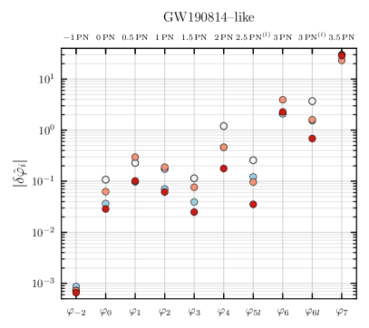
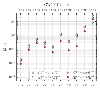
Figure 7: The 90% bounds on the deviation parameters from GW190814–like (left panel) and GW190412–like (right panel) signals when the tapering frequency $f_{22}^{\rm{tape}}$ is varied.

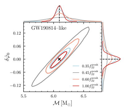
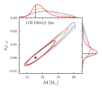
Figure 8: The 2D joint posterior distribution between the deviation parameter $\delta\hat{\varphi}_{0}$ and the chirp mass $\mathcal{M}$ for the results presented in the left and right panels of Fig. 7, respectively. The crosses and vertical dashed lines represent the injected values. The extent of the correlation between the chirp mass and the deviation parameters vary with the tapering frequency.

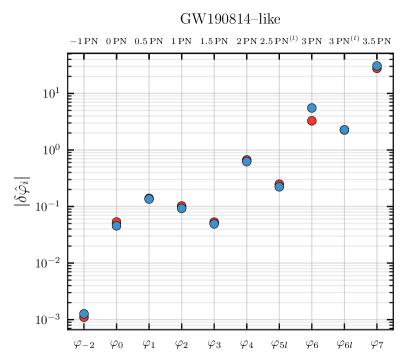
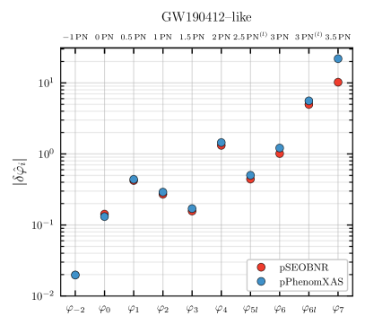
Figure 9: The 90% bounds on the deviation parameters from the simulated GW190814–like (left panel) and GW190412–like (right panel) signals when two waveform families, namely, $\tt{pSEOBNR}$ and $\tt{pPhenomX}$, are used for the recovery.

In this section we would like to investigate how to optimize the null tests enabled by the FTI approach, and also explore possible systematics due to the settings, notably the choice of the tapering frequency, and the family of waveform models adopted.

In Sec. II we have discussed a particular choice of the tapering frequency ($f^{\text{tape}}_{22}=0.35f_{22}^{\rm{peak}}$). Historically, this choice was motivated by comparisons of the FTI results with TIGER results . Nevertheless, given that the FTI method allows for flexibility in the tapering frequency, unlike TIGER, we want to understand the effects of varying it. It is also theoretically difficult to justify exactly where (i.e., at which orbital frequency) the inspiral ends. We thus allow the tapering frequency to vary up until the (approximate) merger frequency, $f_{22}^{\mathrm{peak}}$, and explore its impact on our results. Varying the tapering frequency beyond the merger frequency would not make much sense for an inspiral test. We note that FTI analysis of BNS would not be affected by increasing the default tapering frequency, because for such systems, higher tapering frequency lie outside the sensitivity bandwidth of current GW detectors (e.g., $0.35f_{22}^{\rm{peak}}\simeq 1350$ Hz for GW170817).

Table 2: Fraction of the total SNR between $20$ Hz and the tapering frequency for the two simulated signals emplooyed here.

Tapering frequency	GW190814–like	GW190412–like
0.25$f_{22}^{\rm{peak}}$	83.8%	61.3%
0.35$f_{22}^{\rm{peak}}$	92.1%	76.2%
0.45$f_{22}^{\rm{peak}}$	95.4%	83.2%
0.60$f_{22}^{\rm{peak}}$	97.4%	88.9%
1.00$f_{22}^{\rm{peak}}$	99.3%	96.1%

In Fig. 7 we show the change in the 90% credible intervals of the deviation-parameter posterior distributions, as the tapering frequency is varied. More specifically, the exact change in the bounds depends on the underlying signal itself, for example, for the high–total-mass GW190412–like system (right panel), with less inspiral in the detectors’ frequency bands, bounds on the lower PN order deviation parameters ($\delta\hat{\varphi}_{-2}$, $\delta\hat{\varphi}_{0}$, $\delta\hat{\varphi}_{1}$, $\delta\hat{\varphi}_{2},\hat{\varphi}_{3}$) change at most by a factor of $\sim 2\mbox{-}3$ (if we push the tapering frequency up to the peak of $h_{22}$). This makes sense because those deviation parameters affect the waveform significantly only at low frequencies and thus increasing the tapering frequency does not make much difference to the results. The change on the bounds increases (up to $\sim 5$) for the higher PN deviation parameters, and becomes the largest for $\delta\hat{\varphi}_{6}$, for which the variation is $\sim 7$. Extending the tapering frequency up to close to merger increases the available SNR (see Table 2), and improves the measurement of the higher PN deviation parameters $\delta\hat{\varphi}_{4}$, $\delta\hat{\varphi}_{5\ell}$, $\delta\hat{\varphi}_{6}$.

For low-total-mass GW190814–like systems, as one can see from the left panel of Fig. 7, for almost all deviation parameters, the tapering frequency has a somewhat larger impact on the bounds. Bounds for the lower PN order deviation parameters ($\delta\hat{\varphi}_{-2}$, $\delta\hat{\varphi}_{0}$, $\delta\hat{\varphi}_{1}$, $\delta\hat{\varphi}_{2}$, and $\delta\hat{\varphi}_{3}$) change by a factor of $1\mbox{-}5$, while the higher-order ones change by a factor as large as $\sim 7$ (for $\hat{\varphi}_{5\ell}$). Also in this case, extending the tapering frequency up to merger, can improve the measurement of the high PN deviation parameters. The above studies suggest that to optimize the FTI framework for BBHs, it would be beneficial to obtain a tapering frequency that depends on the available SNR and the number of GW cycles up to the peak of the waveform. Eventually, those quantities depend on the total mass of the binary, mass ratio and spins.

As stated above, the chirp mass $\mathcal{M}$ generally correlates with the deviation parameters, a property discussed in more detail in the following subsection. This means that the measurement of the chirp mass would get affected by the variation of the tapering frequency. This can be seen in Fig. 8. The left panel shows the correlation of $\mathcal{M}$ with $\delta\hat{\varphi}_{0}$ for GW190814–like systems, while the right panel shows the correlation with $\delta\hat{\varphi}_{-2}$ for GW190412–like systems. From the left panel we observe that the variation in the tapering frequency only affects the width of the chirp-mass posterior distribution, while the right panel shows that, additionally, there could arise some biases (even in the deviation parameter $\delta\hat{\varphi}_{-2}$) if the tapering frequency is too low. The reason for this could be that, for relatively high-mass systems, the number of GW cycles in the detectors’ frequency bands is already low to start with, and thus using too low tapering frequencies would essentially make the inference almost insensitive to $\delta\hat{\varphi}_{-2}$. We note that for the GW190412-like source, the bias is quite reduced when we use the tapering frequency at the peak of the (2,2) mode. This is because for this high-mass binary the last few cycles before merger can increase significantly the SNR accumulated. Hence, if one should find evidence for a violation of GR, one must first check for a possible bias of the FTI results by varying the tapering frequency. We find that the other GR parameters, besides the chirp mass, remain mostly unaffected. This could be because they play a subdominant role in the orbital dynamics during the inspiral.

Finally, so far we have employed for our analyses the EOB-based waveform models: $\tt{SEOBNRHM}$ and $\tt{SEOBNR}$. We show in Fig. 9 the results obtained from the two simulated signals when recovered with the aligned-spin phenomenological waveform pPhenomX, in addition to the $\tt{SEOBNR}$ waveform. Both models only contain the $(2,2)$ mode. As we can see, there is really no significant difference between the bounds obtained from these two different waveform families, except for $\delta\hat{\varphi}_{7}$ with the higher-mass GW190412–like system (perhaps due to modeling differences at high frequencies). In addition, the details of the individual posterior distributions (not shown here) are very similar. We thus expect that the results established in this work do not depend much on the underlying family of GR waveform models used, as long as they have comparable accuracy to numerical relativity.

IV.3 Impact of the FTI approach on the GR parameters

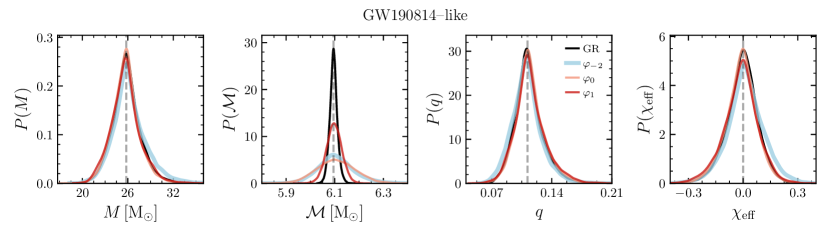
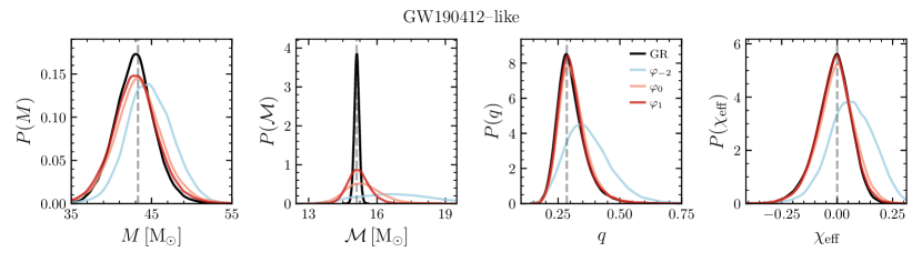
Figure 10: Posterior distributions of several binary’s parameters for the simulated GW190814–like signal (upper panel) and the GW190412–like signal (lower panel) when the GR SEOBNRHM model and the pSEOBNRHM model with deviations parameters $\delta\hat{\varphi}_{-2}$, $\delta\hat{\varphi}_{0}$, and $\delta\hat{\varphi}_{1}$ are used to recover the signal. The vertical dashed lines represent the true value of the injections. The strong correlation between these deviation parameters and the chirp mass $\mathcal{M}$ leads to the broadening of the chirp mass posteriors and sometime causes a bias as well.

In Figs. 10 and 11 we show the posteriors of the GR parameters of the two simulated signals introduced above, when recovering them with the GR SEOBNRHM model and the pSEOBNRHM model. For the cases involving the parameters $\delta\hat{\varphi}_{-2}$ and $\delta\hat{\varphi}_{0}$, we observe that the measurement uncertainty of the chirp mass increases significantly, while other GR parameters, e.g., the total mass ($M$), mass ratio ($q$), or effective spin ($\chi_{\rm{eff}}$), remain unaffected. For the GW190412–like signal, the addition of $\delta\hat{\varphi}_{-2}$ introduces a bias in the measurement of the GR parameters. These biases, however, reduce if a tapering frequency higher than the current default of $0.35f_{22}^{\mathrm{peak}}$ is used for the analysis, as demonstrated in the previous subsection. Hence, the biases appear to be the consequence of an insufficient number of GW cycles or SNR.

The fact that the chirp-mass measurement is heavily correlated or degenerate with the measurement of some non-GR parameters can be understood by looking at the FTI formulation itself. Restricting ourselves to the $(2,2)$-mode, using the definition of $v$ from Eq. (8), the $n/2$-PN-order coefficient in Eq. (11) that contributes to the total phase correction is

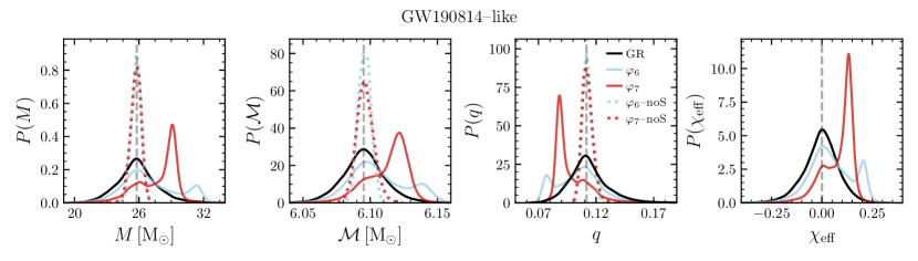
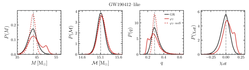
Figure 11: Same as Fig. 10 but for the deviation parameters $\delta\hat{\varphi}_{6}$ and $\delta\hat{\varphi}_{7}$. The dotted lines represent the posteriors obtained with the non-spinning (noS) pSEOBNRHM waveforms. The bimodalities in the GR parameters arise as a consequence of strong correlations between masses and spins induced by the deviation parameters $\delta\hat{\varphi}_{6}$ and $\delta\hat{\varphi}_{7}$.

$$\psi_{n}(f;\bm{\theta})=\dfrac{3}{128(\mathcal{M}\pi f)^{5/3}}\,\psi_{n}^{(\text{GR})}(\bm{\theta})(1+\delta\hat{\varphi}_{n}),$$ (19)

where $\delta\hat{\varphi}_{n}$ is the $n/2$-PN-order deviation parameter. For the leading-order term $n=0$, this implies

$$\psi_{0}(f;\bm{\theta})=\dfrac{3}{128(\mathcal{M}\pi f)^{5/3}}\,(1+\delta\hat{\varphi}_{0})$$ (20)

since $\psi_{0}^{(\text{GR})}=1$. For the -1PN and 0.5PN phase corrections (i.e., $n=-2,1$), which are absolute corrections since they are absent in GR, the expressions read

$$\psi_{-2}(f;\bm{\theta})=\dfrac{3}{128(\mathcal{M}\pi f)^{5/3}}\,\delta\hat{\varphi}_{-2},$$ (21)

and

$$\psi_{1}(f;\bm{\theta})=\dfrac{3}{128(\mathcal{M}\pi f)^{5/3}}\,\delta\hat{\varphi}_{1}.$$ (22)

It becomes clear from Eqs. (20), (21), and (22) that the deviation parameters $\delta\hat{\varphi}_{-2}$, $\delta\hat{\varphi}_{0}$ and $\delta\hat{\varphi}_{1}$ are degenerate with the chirp mass, as Fig. 8 shows. There are also correlations between the chirp mass (and other binary parameters) and the deviation parameters at higher PN orders, but they are milder. Indeed the addition of $\delta\hat{\varphi}_{2}$, $\delta\hat{\varphi}_{3}$, $\delta\hat{\varphi}_{4}$, $\delta\hat{\varphi}_{5l}$ and $\delta\hat{\varphi}_{6l}$ do not affect estimates of GR parameters in any noticeable fashion, as we have verified using the results in Figs. 10 and 11.

However, for the highest PN-order deviation parameters, $\delta\hat{\varphi}_{6}$ and $\delta\hat{\varphi}_{7}$, posterior distributions of GR parameters can show features like bimodalities, depending on the underlying signal, see Fig. 11. This is because, unlike the cases of $n=-2,0,1$, for values of $n\geq 2$ the PN coefficients $\psi_{n}^{(\text{GR})}$ also depend on the intrinsic properties, in particular the symmetric mass ratio and the spins. In fact, the bimodalities observed in the $\delta\hat{\varphi}_{6}$ and $\delta\hat{\varphi}_{7}$ cases disappear when we perform the analysis with non-spinning waveforms, shown by the dotted lines in Fig. 11. This suggests that the deviation parameters $\delta\hat{\varphi}_{6}$ and $\delta\hat{\varphi}_{7}$ induce strong correlations between the GR parameters when the binary is spinning. We notice that the amount of bimodality also depends on the tapering frequency, notably on the GW cycles and SNR.

V Application of the FTI approach to a binary neutron star

Here we consider the application of the FTI approach to a specific alternative theory of GR: the Jordan–Fierz–Brans–Dicke (JFBD) scalar–tensor theory Jordan (1955); Fierz (1956); Brans and Dicke (1961). Initially formulated in the mid-20th century, JFBD gravity was the very first scalar-tensor theory—a theory in which gravity is mediated by both a tensor (the metric) and a scalar. Since then, significant work has been done to extend this notion beyond JFBD theory to broader, more generic classes of scalar-tensor theories (e.g., Horndeski theories Horndeski (1974), Beyond Horndeski theories Gleyzes et al. (2015), Degenerate Higher-Order Scalar-Tensor theories Langlois and Noui (2016); Langlois (2017)). Yet, despite its simplicity, JFBD gravity remains relevant today, though more as a pedagogical archetype of modified gravity than as a truly viable alternative to GR. In this vein, constraining JFBD theory with a particular experiment offers an easily understood benchmark of its sensitivity to deviations from GR.

The action for JFBD gravity written in the Jordan frame is given by

$$S=\int d^{4}x\frac{\sqrt{-\tilde{g}}}{16\pi}\left(\phi\tilde{R}-\frac{\omega_{\text{BD}}}{\phi}\tilde{g}^{\mu\nu}\partial_{\mu}\phi\partial_{\nu}\phi\right)+S_{m}[\tilde{g}_{\mu\nu},\psi],$$ (23)

where $\phi$ is a massless scalar field, $\omega_{\text{BD}}$ is a dimensionless coupling constant, and $S_{m}$ represents the action for matter fields $\psi$ minimally coupled to the metric $\tilde{g}_{\mu\nu}$. (Here $\psi$ should not be confused with the GW modes $\psi_{\ell m}$ introduced earlier.) Alternatively, the action can be rewritten in the Einstein frame by performing the conformal transformation $g_{\mu\nu}\equiv\phi\tilde{g}_{\mu\nu}$

$$S=\int d^{4}x\frac{\sqrt{-g}}{16\pi}\left(R-2g^{\mu\nu}\partial_{\mu}\varphi\partial_{\nu}\varphi\right)+S_{m}[e^{-2\alpha_{0}\varphi}g_{\mu\nu},\psi],$$ (24)

where we have defined the dimensionless parameter $\alpha_{0}\equiv(3+2\omega_{\text{BD}})^{-1/2}$ and introduced the scalar field $\varphi\equiv\log(\phi)/(2\alpha_{0})$; note that $\alpha_{0}$ is non-negative and that we have implicitly assumed that $\omega_{\text{BD}}>-3/2$. (Note that $\varphi$ is unrelated to the FTI deviation parameters.) In the limit that $\alpha_{0}\rightarrow 0$ ($\omega_{\text{BD}}\rightarrow\infty$), the scalar field decouples from the metric and matter, and JFBD theory reduces to GR with an additional massless scalar that is minimally coupled to gravity only. The most accurate constraints on this parameter come from the Doppler tracking of the Cassini spacecraft through the Solar System Bertotti et al. (2003) $\alpha_{0}<4\times 10^{-3}$ ($\omega_{\text{BD}}>4\times 10^{4}$), and binary pulsar obervations Damour and Esposito-Farese (1992, 1993); Wex (2014); Anderson et al. (2019). In particular, the most recent results obtained in Ref. Kramer et al. (2021) with 16 years of observation of the double-pulsar J0737-3039 yield the bounds $\alpha_{0}=0.004083$, and $=0.003148$ at $95\%$ credible level, when the stiff MPA1 and soft WFF1 EOS are employed, respectively.

The recent advent of GW astronomy offers a new avenue to test gravity in the relativistic regime. The majority of GWs observed by LIGO and Virgo thus far were generated by the coalescence of BBHs; several tests of GR have already been conducted using these observations Abbott et al. (2016b, c); Yunes et al. (2016); Abbott et al. (2019). However, Hawking famously showed that stationary BHs in JFBD theory must have a trivial scalar profile, and thus are indistinguishable from the analogous solutions in GR Hawking (1972). Although there are some possible scenarios that evade this no-hair theorem (see, e.g., Ref. Sotiriou (2015)), binary systems composed of BHs are generally expected to behave identically in JFBD theory and GR, and thus GWs from such systems are unable to constrain this scalar-tensor theory.

Unlike BHs, NSs source a nontrivial scalar field in JFBD gravity, and thus BNS systems can be used to constrain $\alpha_{0}$. In this section, we use the first GW observation of a coalescing BNS—GW170817 Abbott et al. (2017a)—to constrain $\alpha_{0}$ at the 68% (and 90%) credible levels. Though the constraint from GW170817 is not as strong as those previously quoted from other experiments, this result represents the first bound directly from the highly dynamical (orbital velocities $v\sim 10^{-1}$) and strong-field (Newtonian potential $\Phi_{\text{Newt}}=M/R\sim 10^{-1}$) regime of gravity.

This section is organized as follows. In Sec. V.1, we detail the GW signature of JFBD theory in BNSs. Then, in Sec. V.2, we present two Bayesian analyses to constrain $\alpha_{0}$ with GW170817: the first directly uses the theory-agnostic analyses presented in Sec. II, while the second is tailored specifically to test JFBD gravity.

V.1 Gravitational-wave signature of JFBD gravity

The predominant differences in GWs produced in JFBD gravity as compared to GR stem from the fact that only the latter respects the strong equivalence principle. This principle extends the universality of free fall by test particles implied by the Einstein equivalence principle to also include self-gravitating bodies; unlike in GR, the motion of a body through spacetime depends on its internal gravitational interactions (i.e., its composition) in scalar-tensor theories like JFBD gravity. This section details how this violation of the strong equivalence principle impacts the GWs produced by binary systems in JFBD gravity. This alternative theory of gravity falls within the class of scalar-tensor theories for which PN predictions have been computed. Though those results are available at next-to-next-to-leading PN order (and even higher-order PN calculations have been made recently Sennett et al. (2016); Bernard (2018, 2019); Bernard et al. (2022)), we will assume that $\alpha_{0}$ is sufficiently small that we can neglect all but the leading-order PN effects when describing the signature of JFBD gravity in a gravitational waveform.

Table 3: One-dimensional polynomial fits of the normalized NS coupling $\alpha_{i}/\alpha_{0}$ as a function of NS mass $m_{i}$ (in units of $M_{\odot}$) for various EOSs. The relative error amounts to less than 5% over the area $(m_{i},\alpha_{0})\in[0.5\,M_{\odot},2.0\,M_{\odot}]\times[0.001,1.0]$.

EOS		fit for $[\alpha_{i}/\alpha_{0}](m_{i})$
sly	Douchin and Haensel (2001)	$-0.726798$	$-0.749029\,m_{i}$	$+1.270944\,m_{i}^{2}$	$-0.728710\,m_{i}^{3}$	$+0.161002\,m_{i}^{4}$
eng	Engvik et al. (1996)	$-0.817884$	$-0.393375\,m_{i}$	$+0.772615\,m_{i}^{2}$	$-0.435306\,m_{i}^{3}$	$+0.095059\,m_{i}^{4}$
H4	Lackey et al. (2006)	$-0.613880$	$-1.210074\,m_{i}$	$+1.836631\,m_{i}^{2}$	$-1.056595\,m_{i}^{3}$	$+0.228102\,m_{i}^{4}$

Table 4: Two-dimensional polynomial fits of the normalized NS coupling $\alpha_{i}/\alpha_{0}$ as functions of the Brans-Dicke parameter $\alpha_{0}$ and NS mass $m_{i}$ (in units of $M_{\odot}$) for various EOSs. The relative error amounts to less than 1% over the area $(m_{i},\alpha_{0})\in[0.5\,M_{\odot},2.0\,M_{\odot}]\times[0.001,1.0]$.

EOS		fit for $[\alpha_{i}/\alpha_{0}](m_{i},\alpha_{0})$
sly	Douchin and Haensel (2001)	$-0.92569$		$+0.22258\,\alpha_{0}m_{i}$	$+0.13329\,m_{i}^{2}$	$-0.15151\,\alpha_{0}m_{i}^{2}$
eng	Engvik et al. (1996)	$-0.97423$	$+0.15584\,m_{i}$	$+0.18527\,\alpha_{0}m_{i}$		$-0.11739\,\alpha_{0}m_{i}^{2}$	$+0.024333\,m_{i}^{3}$
H4	Lackey et al. (2006)	$-0.93341$		$+0.19073\,\alpha_{0}m_{i}$	$+0.10270\,m_{i}^{2}$	$-0.11284\,\alpha_{0}m_{i}^{2}$

The dominant effect on the inspiral from the new scalar introduced in JFBD gravity is the emission of dipole radiation, which enters into the phase evolution at -1PN order. In the notation of the FTI framework and using the fact that the quadrupolar GR radiation dominates over the dipolar one for small $\alpha_{0}$ Sennett et al. (2016), this contribution is given by

$$\delta\hat{\varphi}_{-2}=-\frac{5(\alpha_{1}-\alpha_{2})^{2}}{168}+\mathcal{O}\left(\alpha_{0}^{4}\right),$$ (25)

where $\alpha_{i}$ is the scalar charge of body $i$, defined as

$$\alpha_{i}\equiv-\frac{d\log m_{i}(\varphi)}{d\varphi},$$ (26)

where $m_{i}(\varphi)$ is the gravitational mass of body $i$ measured in the Einstein frame ($i=1,2$). That a body’s mass depends on the local value of the scalar field is unsurprising given the form of Eq. (24); a shift in $\varphi$ modulates the physical metric $e^{-2\alpha_{0}\varphi}g_{\mu\nu}$ that effects gravity upon the matter fields $\psi$, and thus also modulates any body’s gravitational mass. This dependence is an explicit manifestation of violation of the strong equivalence principle. Note that in the limit that a body has no self-gravity (i.e., the test-body limit), the functional form of $m_{i}(\varphi)$ simplifies significantly to

$$m_{i}^{\text{(test body)}}(\varphi)=e^{-\alpha_{0}\varphi}m_{i}^{\text{(test body)}}(\varphi=0),$$ (27)

and thus its scalar charge reduces to

$$\alpha_{i}^{\text{(test body)}}=\alpha_{0}.$$ (28)

As strongly self-gravitating bodies, violations of the strong equivalence principle are particularly pronounced in NSs. This violation manifests as a scalar charge that differs significantly from the test-body charge $\alpha_{0}$. As the scalar charges of a binary’s constituents—or rather their difference, the scalar dipole—control the dominant effect on the GW signal in JFBD gravity, we devote the remainder of this subsection to computing these quantities for various NSs.

We consider spherically symmetric, static solutions sourced by a perfect fluid as a model for an isolated, nonspinning NS. Under these assumptions, the field equations for Eq. (24) reduce to the Tolman-Oppenheimer-Volkoff (TOV) equations, given in the Einstein frame in Ref. Damour and Esposito-Farese (1993). These solutions are parameterized by three degrees of freedom; for our purposes, these are most clearly manifested as the (i) background scalar field $\varphi_{0}$, that is the scalar field far from the NS, (ii) the NS EOS, and (iii) the NS mass. Note that the asymptotic scalar field $\varphi_{0}$ can be set to zero without loss of generality by rescaling the Jordan-frame bare gravitational constant $\tilde{G}$ accordingly, that is $\varphi_{0}\rightarrow 0\Rightarrow\tilde{G}\rightarrow\tilde{G}e^{2\alpha_{0}\varphi_{0}}$. The remaining degrees of freedom can be mapped to boundary conditions for the matter and scalar field at the origin with a numerical shooting method Press et al. (1992). These conditions are parameterized by the central pressure $P_{c}$ and the scalar field $\varphi_{c}$, which serve as the inputs for numerically integrating the TOV equations. (Note that in this section $\varphi_{c}$ is different from the parameter used in Sec. II to define the binary’s orientation.) The details for extracting the mass and scalar charge from the numerical solutions of the NS interior are given in Ref. Damour and Esposito-Farese (1993).

Ultimately, we would like to combine the numerical calculations of the NS scalar charge outlined above with their anticipated effect on the GW signal (25) to constrain JFBD theory. However, evaluating the scalar charge directly for every point visited by the stochastic sampling algorithms used for parameter estimation would require an unreasonable amount of computational resources. Instead, we compute polynomial fits for the scalar charge, which, after having been derived, can be evaluated quickly and with little computational overhead.

We first construct solutions for various choices of EOS, NS mass, and scalar-tensor coupling $\alpha_{0}$. We interpolate tabulated EOS data for the sly Douchin and Haensel (2001), eng Engvik et al. (1996), and H4 Lackey et al. (2006) EOSs; sly is a soft EOS (compact stars) whereas H4 is relatively stiff (diffuse stars). Then, we numerically construct NSs with masses ranging between ${m_{i}\in[0.5\,M_{\odot},2.0\,M_{\odot}]}$ and scalar coupling ${\alpha_{0}\in[0.001,1.0]}$ and compute their scalar charge.

We calculate two types of polynomial fits of the scalar charge for each EOS. For the first, we factor out the dominant linear dependence of $\alpha_{i}$ on $\alpha_{0}$, fitting their quotient as a fourth-order polynomial in $m_{i}$. We compute the polynomial fits with least-squares regression; the fits are given in Table 3 for each EOS that we consider. These fits match all of our data sets within 5% relative error, with the greatest discrepancy arising for masses close to $2\,M_{\odot}$.

Although these (effectively) one-dimensional polynomial fits are crucial for some of our analysis, it is possible to construct two-dimensional fits that are simpler (fewer terms) and more accurate using more sophisticated methods. We compute these fits using the greedy-multivariate-rational regression method developed in Ref. London and Fauchon-Jones (2018). This method relies on a greedy algorithm to construct a multivariate fit: during each iteration, it adds a polynomial term to the current fit (up to a pre-specified maximum degree) so as to best improve the agreement with the inputted data. This process is repeated until sufficient accuracy is achieved, and then terms are systematically removed from the polynomial until the accuracy goal is saturated. Using this method, we construct fits that agree to within 1% relative error for each EOS—these are listed in Table 4.

V.2 Constraining $\alpha_{0}$ with GW170817

Next, we use the tools introduced previously to place constraints on the scalar-tensor coupling $\alpha_{0}$ in JFBD gravity with GW170817—the first GW event from a coalescing BNS. We present two complementary analyses based off of the FTI infrastructure to achieve this result. These two methods follow the same overall approach, but adopt different statistical assumptions, utilize different waveform models, and use different numerical fits for the NS scalar charge $\alpha_{i}$. In both approaches, we employ a generalized waveform model that allows for an additional contribution to the phase evolution at -1PN order, so as to reproduce the behavior seen in Eq. (25); however, the parameterization of this -1PN deviation from GR differs in each approach. Ultimately, both analyses provide a bound on $\alpha_{0}$ of the same order of magnitude.

The first approach we adopt directly uses the theory-agnostic constraints on a -1PN deviation, and it was originally obtained in Ref. Abbott et al. (2018b). We use in this analysis a generalization of the tidal, aligned-spin SEOBNRT Bohé et al. (2017); Hinderer et al. (2016); Lackey et al. (2019) waveform model in which the -1PN term is parameterized by the deviation parameter $\delta\hat{\varphi}_{-2}$. By assuming a particular NS EOS, we can use the polynomial fit in Table 3 in conjunction with Eq. (25) to map a measured value of $\delta\hat{\varphi}_{-2}$ to an inferred value on $\alpha_{0}$; schematically, this mapping takes the form $\alpha_{0}(\delta\hat{\varphi}_{-2},m_{1},m_{2};\text{EOS})$. Note that this mapping is infeasible using the multivariate fit in Table 4 because of the nonlinear dependence of $\alpha_{i}$ on $\alpha_{0}$. Though the exact NS EOS remains unknown, we can repeat this analysis for the three candidate EOSs detailed earlier, and then use the variance on the bounds of $\alpha_{0}$, recovered each time, as an estimate of the systematic error arising from our ignorance of the true NS EOS.

In practice, one does not measure the masses and deviation parameter $\delta\hat{\varphi}_{-2}$ with perfect accuracy, but instead uses Bayesian inference (Sec. III) to reconstruct the posterior distribution $P(\bm{\theta}|d,\mathcal{H})$ on these parameters given some assumed prior distribution $p(\bm{\theta}|\mathcal{H})$. So, rather than map a single point from one parameterization to another, we instead map the appropriate distributions to their counterparts in the new parameterization. These prior and posterior distributions transform respectively as

$$\begin{split}p(\alpha_{0},m_{1},m_{2}|\mathcal{H})=\left|\frac{\partial(\alpha_{0},m_{1},m_{2})}{\partial(\delta\hat{\varphi}_{-2},m_{1},m_{2})}\right|^{-1}\\ \times p(\delta\hat{\varphi}_{-2},m_{1},m_{2}|\mathcal{H}),\end{split}$$ (29)

and

$$\begin{split}P(\alpha_{0},m_{1},m_{2}|d,\mathcal{H})=\left|\frac{\partial(\alpha_{0},m_{1},m_{2})}{\partial(\delta\hat{\varphi}_{-2},m_{1},m_{2})}\right|^{-1}\\ \times P(\delta\hat{\varphi}_{-2},m_{1},m_{2}|d,\mathcal{H}),\end{split}$$ (30)

where the first term on the right-hand side of either equations is the inverse of the Jacobian of the aforementioned transformation.

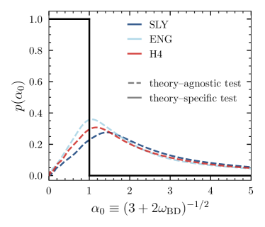
Figure 12: Marginalized prior distributions on the JFBD parameter $\alpha_{0}$ used in the two analyses. The dashed colored curves depict the prior distribution equivalent to the flat prior distribution on component masses and deviation parameter $\delta\hat{\varphi}_{-2}$ assumed in the theory-agnostic analysis. The solid black curve depicts the flat prior on $\alpha_{0}$ assumed in the theory-specific test.

In the analysis of Ref. Abbott et al. (2018b), a flat prior was assumed on the component masses and deviation parameter $\delta\hat{\varphi}_{-2}$. (We note that the upper prior bound is dictated by the theory since $\delta\hat{\varphi}_{-2}\leq 0$, see Eq. (25).) These choices reflect the theory-agnostic nature of that test; without a preferred alternative, this choice represents the simplest prior in terms of these binary parameters. Figure 12 depicts with dashed lines how this choice of prior distribution maps to an assumed prior on $\alpha_{0}$ through Eq. (29); here the different colors correspond to different assumed EOSs. Similarly, the dashed lines in Fig. 13 show the corresponding marginalized posteriors on $\alpha_{0}$, transformed from the posterior on $\delta\hat{\varphi}_{-2}$ and component masses via Eq. (30). This analysis provides a bound of $\alpha_{0}\lesssim 2\times 10^{-1}$ ($5\times 10^{-1}$) at a 68% (90%) credible level. We find that that the systematic error arising from our ignorance of the NS EOS does not impact our estimate at 68%, but change the bound at 90% CL by $\sim 30\%$. The bound on $\alpha_{0}$ with GW170817 is about three orders of magnitude larger than what obtained with the double-pulsar J0737-3039 Kramer et al. (2021), which since 2003 has been tracked for about 60 000 orbital cycles. Future observations with GW detectors on the ground and in space, will allow to reach similar or better accuracies Perkins et al. (2021b). Due to the much smaller velocity ($v/c\sim 2\times 10^{-3}$), the double-pulsar observation becomes quickly less constraining for high PN terms entering the GW phasing (i.e., the ones discussed in Sec. IV).

We can straightforwardly translate our bounds on the coupling to the JFBD parameter $\omega_{\text{BD}}$ using that $\alpha_{0}^{2}=1/(3+2\omega_{\text{BD}})$, see Table 5. We find that the conservative bound in the theory-specific approach is $\omega_{\text{BD}}\gtrsim 1.12$ $(-0.70)$ at a 68% (90%) credible level. We also find it useful to quote here a bound on the parameterized post-Newtonian (PPN) parameter $\gamma_{\text{PPN}}$ Anderson et al. (2019) that would correspond to our bound on $\alpha_{0}$, using $|1-\gamma_{\text{PPN}}|=2\alpha_{0}^{2}/(1+\alpha_{0}^{2})$. This leads us to the bound $|1-\gamma_{\text{PPN}}|\lesssim 0.32$ $(0.77)$ at a 68% (90%) credible level. However, note that our constraint originates from the dipole radiation and not from the 1PN deformation of the metric that defines $\gamma_{\text{PPN}}$.

Table 5: Our bounds on the coupling $\alpha_{0}$ translated to bounds on the JFBD parameter $\omega_{\text{BD}}$ and the PPN parameter $\gamma_{\text{PPN}}$. The numbers here indicate 68% credible level, while the numbers in brackets are the 90% credible level.

theory-specific bounds
EOS		$\omega_{\text{BD}}$	$|1-\gamma_{\text{PPN}}|$
sly	Douchin and Haensel (2001)	1.69 (-0.68)	0.27 (0.76)
eng	Engvik et al. (1996)	1.12 (-0.70)	0.32 (0.77)
H4	Lackey et al. (2006)	1.20 (-0.69)	0.31 (0.76)

theory-agnostic bounds
EOS		$\omega_{\text{BD}}$	$|1-\gamma_{\text{PPN}}|$
sly	Douchin and Haensel (2001)	25.17 (1.00)	0.04 (0.33)
eng	Engvik et al. (1996)	18.69 (0.42)	0.05 (0.41)
H4	Lackey et al. (2006)	14.37 (-0.02)	0.06 (0.50)

The second approach we employ to constrain $\alpha_{0}$ relies instead on a waveform model design specifically to test JFBD theory. Using the FTI infrastructure, we construct a generalized waveform model from SEOBNRT in which the deviation parameter is precisely $\alpha_{0}$. The appropriate form of the -1PN correction to the phase evolution is obtained by inserting the polynomial fit for $\alpha_{i}(\alpha_{0},m_{i})$ found in Table 4 for a particular choice of the EOS into Eq. (25). Additionally, unlike the previous theory-agnostic analysis in which the tidal parameters were allowed to vary freely, for this analysis, we express these parameters as functions of the respective NS masses and assumed EOS. This step reduces the dimensionality of the waveform model by two parameters while ensuring that all matter effects are handled self-consistently. We assume a flat prior on $\alpha_{0}\in[0,1]$ for this analysis; beyond this upper bound, our assumption that JFBD effects of order $\alpha_{0}^{2}$ are subdominant to the PN effects in GR is no longer valid. This prior distribution is depicted in Fig. 12 with a solid black curve. Using the generalized waveform described above, we perform parameter estimation to construct the marginalized posterior distribution on $\alpha_{0}$, shown in Fig. 13 with solid colored curves corresponding to the assumed EOS. We obtain the upper bound of $\alpha_{0}\lesssim 4\times 10^{-1}$ ($8\times 10^{-1}$) at a 68% (90%) credible interval where, as before, the systematic error due to ignorance of the true NS EOS does not contribute at this level of precision. As explained above, our constraint on $\alpha_{0}$ can be translated to the bounds $\omega_{\text{BD}}\gtrsim 14.37$ $(-0.02)$ or $|1-\gamma_{\text{PPN}}|\lesssim 0.06$ $(0.50)$ at a 68% (90%) credible level.

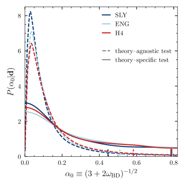
Figure 13: Marginalized posterior distributions on the JFBD parameter $\alpha_{0}$ recovered from GW170817. The dashed curves show the posterior recovered directly from the theory-agnostic analysis. The solid curves depict the posterior using the theory-specific test of JFBD assuming a flat prior for $\alpha_{0}$. For both analyses, different colors correspond to different assumed EOSs. The short vertical lines on the horizontal axes represent the 90% upper bounds on $\alpha_{0}$ for each analysis. The theory-agnostic test provides better bounds on $\alpha_{0}$.

Comparing the bounds set by the two analyses, we see that the theory-agnostic test provides a stronger bound on $\alpha_{0}$. At first glance, this result may appear counterintuitive, as Fig. 12 shows that this test assumed a marginalized prior on $\alpha_{0}$ with greater support away from zero. The predominant cause for this discrepancy stems from how the tidal parameters are handled by each waveform model. For the theory-agnostic test, these parameters are allowed to vary freely, independent of the masses of the NSs. However, in the theory-specific test, the tidal parameters are linked directly to the component masses. This latter restriction significantly affects the recovered posterior distribution on the component masses, placing much greater weight near equal-mass configurations than in the previous case. As can be seen in Eq. (25), in very symmetric configurations, the total deviation from the baseline GR waveform remains small even when $\alpha_{0}$ is relatively large; as a result, the JFBD parameter is more poorly measured when the tidal parameters cannot vary freely, and thus we recover a weaker bound with this theory-specific test.

VI Conclusion

In this paper we have developed a framework that allows us to introduce deviations from GR to any frequency-domain inspiral phasing, assuming that such corrections are small modifications to the GR signal. For theory-agnostic tests, our FTI framework has already been successfully applied to GWs observed by LIGO and Virgo detectors by the LVC in Refs. Abbott et al. (2016b, c, 2018b, 2019, 2021f, 2021g), while for theory-specific tests the FTI method was employed in Ref. Sennett et al. (2020) to set bounds on an effective-field theory of GR using BBH signals.

More specifically, building on the PN SPA phasing in frequency domain, we have described how to apply the FTI framework to multipolar aligned-spin waveforms, by introducing deviations parameters to GR PN terms up to 3.5PN order, and also to PN terms that are absent in GR, such as the -1PN and 0.5PN corrections. Although we apply our framework mainly to the inspiral-merger-ringdowm SEOBNRHM waveform model, which contains $(\ell,m)=(2,1),(3,3),(4,4),(5,5)$ modes in addition to the dominant $(2,2)$ mode, the method is general and can be used for any frequency-domain waveform (or the Fourier-transform of a time-domain waveform). The corrections introduced in the phasing are tapered off at a certain orbital frequency, which is a free parameter in this framework. The tapering process is introduced to ensure that the modified PN phase for each mode reduces to its corresponding GR phase during the late-inspiral–merger-ringdown stages, up to a constant phase shift above the tapering frequency.

We have then discussed the application of the FTI framework to BBHs, notably to two specific high–mass-ratio events observed by LIGO and Virgo, GW190412 and GW190814. The latter were previously analyzed in Ref. Abbott et al. (2021f), where it was observed that the posterior distributions of the -1PN deviation parameter, $\delta\hat{\varphi}_{-2}$, were peaking away from the GR prediction, suggesting possible modeling systematic biases. Here, by creating simulated signals with parameters corresponding to the median values of the two events, we have demonstrated that these features are most likely due to (unexplored) artifacts of the noise around the events rather than missing physics in the waveform models. Furthermore, using the simulated signals, we have showed that modes beyond the quadrupole do affect the accuracy of the deviation-parameter measurements and the GR parameters, especially if the signals have relatively high-mass ratios and inclinations. In such cases, neglecting the high modes can significantly bias the measurements at high SNRs, leading, erroneously, to interpret the measurement results as a violation of GR.

We have also performed robustness tests of the FTI results, and showed that the bounds could be sensitive to the tapering frequency, depending on the parameters of the signal being analyzed. For very low total-mass systems like the BNS GW170817, the tapering frequency lies outside the frequency band where the majority of the SNR is accumulated, thus the bounds are not expected to change. On the other hand, for high–total-mass BBH systems, like GW190814 and GW190412, the bounds on the deviation parameters can change. More specifically, bounds on deviation parameters that are measured with an accuracy of few tens of percent or less, may change by a factor $2\mbox{--}5$, depending on the binary’s parameters, when the tapering frequency spans the last $3\mbox{--}4$ GW cycles before the (2,2)-mode’s peak. These results suggest to go beyond the choice of the tapering frequency adopted so far in Refs. Abbott et al. (2016b, c, 2018b, 2019, 2021f), where it was fixed to a specific value to compare with the complimentary analysis provided by the TIGER framework Agathos et al. (2014). In order to optimize the GR test with the FTI and exploit the full SNR accumulated during the inspiral, up to merger, comprehensive studies would need to be undertaken to determine the best choice of the tapering frequency as a function of the binary’s properties and the accumulated SNR. By contrast, we have shown that the bounds are marginally affected by the use of a different but similarly accurate waveform model, e.g., the state-of-the-art aligned-spin (phenomenological) pPhenomX model, instead of pSEOBNR.

Moreover, we have investigated how the presence of the deviation parameters in the waveform model affects the measurement of the GR parameters. We have found that most deviation parameters such as $\delta\hat{\varphi}_{2}$, $\delta\hat{\varphi}_{3}$, $\delta\hat{\varphi}_{4}$, $\delta\hat{\varphi}_{5l}$, and $\delta\hat{\varphi}_{6l}$ do not impact the GR parameters in any noticeable way. On the other hand, the lower-order deviation parameters $\delta\hat{\varphi}_{-2}$, $\delta\hat{\varphi}_{0}$ and $\delta\hat{\varphi}_{1}$ affect the width of the chirp-mass measurement quite significantly. This is due to the fact that those deviation parameters are degenerate with the chirp mass. We have found that the extent of the correlation, however, also depends on the choice of the tapering frequency (i.e., on the amount of SNR). The remaining two deviation parameters, $\delta\hat{\varphi}_{6}$ and $\delta\hat{\varphi}_{7}$, can cause bimodalities in the posterior distributions of the GR parameters. The strength of these bimodalities depends on the tapering frequency and the binary’s parameters. We find that the bimodalities can be also caused by the fact that the 3PN and 3.5PN terms in the phasing are functions of the mass ratio and the spins, and depending on the binary’s parameters, those PN coefficients can go to zero. It might be possible to avoid bimodalities in the GR posterior distributions by splitting the deviation parameters at 3PN and 3.5PN order in non-spinning and spinning parts, and do inference on those parts separately.

Finally, we have used the FTI method to perform a theory-specific test with the BNS event GW170817 and the JFBD gravity theory. We have obtained constraints on the JFBD parameter $\alpha_{0}$ following two strategies and employing the tidal aligned-spin SEOBNRT waveform model. In the first approach, we directly converted the theory-agnostic -1PN (i.e., $\delta\hat{\varphi}_{-2}$) posterior samples into samples of $\alpha_{0}(\delta\hat{\varphi}_{-2},m_{1},m_{2};\text{EOS})$ using the fits in Table 3 for different NS EOSs. This approach has provided us with a bound on $\alpha_{0}\lesssim 2\times 10^{-1}$ ($5\times 10^{-1}$) at the 68% (90%) credible interval, see also Table 5 for the corresponding bounds on $\omega_{\text{BD}}$ and $\gamma_{\text{PPN}}$. In the second approach, we have employed a waveform model that is specifically designed to test JFBD, that is we have chosen as deviation parameter directly $\alpha_{0}$. In this case, the phase corrections are given by Eq. (25) where $\alpha_{1}$ and $\alpha_{2}$ are determined using the fits in Table 4. Additionally, in this second approach, we have also fixed the tidal parameters since for a given EOS they can be determined from the component masses. This process reduces the dimensionality of the waveform model while ensuring that all matter effects are handled self-consistently. Using a flat prior on $\alpha_{0}\in[0,1]$, we have found a bound on $\alpha_{0}\lesssim 4\times 10^{-1}$ ($8\times 10^{-1}$) at the 68% (90%) credible interval, see also Table 5 for the corresponding bounds on $\omega_{\text{BD}}$ and $\gamma_{\text{PPN}}$. The main reason for the difference in the bounds can be traced to how the tidal parameters are handled in the two approaches. In the theory-agnostic approach the tidal parameters were allowed to vary freely during the inference analysis. By contrast, in the theory-specific approach, tidal parameters and scalar sensitivities cannot be treated as independent, but must be computed consistently (for each NS mass) by fixing the EOS. Thus, theory-specific and theory-agnostic analyses test slightly different statistical hypotheses, and within a fully Bayesian framework, converting results from one to the other requires care. To our knowledge, the impact of statistical hypotheses on relating theory-specific and theory-agnostic bounds has not been studied in detail in the context of GW tests of GR, and thus offers an interesting new avenue for future work.

Lastly, the FTI framework can be applied to perform theory-specific tests with non-GR theories other that JFBD gravity, as done in Ref. Sennett et al. (2020). Additionally, the framework can be adapted to constrain other effects that leave an impact on the inspiral phase — for example the existence of exotic compact objects having a spin-induced quadrupole moment different from the one of a BH in GR Krishnendu et al. (2017); Narikawa et al. (2021). However, more crucial for future, more sensitive observations, is the extension of the FTI framework to the spin-precessing case. This will be possible by applying the frequency-domain corrections to the phasing in the co-precessing frame, where the GWs are usually well approximated by aligned-spin waveforms Buonanno et al. (2003); Ossokine et al. (2020).

Appendix A The 3.5 PN phasing in the stationary-phase approximation

Here, we write the PN coeffcients entering the GW phasing in the SPA approximation Sathyaprakash and Dhurandhar (1991) through 3.5PN order, including spin effects in GR.

Let us introduce the following quantities:

$$\delta=\dfrac{(m_{1}-m_{2})}{M}=1-4\nu,$$ (31a)

$$\chi_{\rm S}=\dfrac{(\chi_{1}+\chi_{2})}{2},$$ (31b)

$$\chi_{\rm A}=\dfrac{(\chi_{1}-\chi_{2})}{2},$$ (31c)

and the Euler’s constant $\gamma_{\rm E}$. The PN coefficients in Eq. (7) read Buonanno et al. (2009); Arun et al. (2009); Bohé et al. (2013):

$$\psi_{0}=1,$$ (32a)

$$\psi_{1}=0,$$ (32b)

$$\psi_{2}=\dfrac{3715}{756}+\dfrac{55\nu}{9},$$ (32c)

$$\psi_{3}=-16\pi+\frac{113\delta\,\chi_{\rm A}}{3}+\left(\frac{113}{3}-\frac{76\nu}{3}\right)\chi_{\rm S},$$ (32d)

$$\psi_{4}=\frac{15293365}{508032}+\frac{27145\nu}{504}+\frac{3085\nu^{2}}{72}+\left(-\frac{405}{8}+200\nu\right)\chi_{\rm A}^{2}-\frac{405\delta\,\chi_{\rm A}\,\chi_{\rm S}}{4}+\left(-\frac{405}{8}+\frac{5\nu}{2}\right)\chi_{\rm S}^{2},$$ (32e)

$$\psi_{5}=\frac{38645\pi}{756}-\frac{65\pi\nu}{9}+\left(-\frac{732985}{2268}-\frac{140\nu}{9}\right)\delta\,\chi_{\rm A}+\left(-\frac{732985}{2268}+\frac{24260\nu}{81}+\frac{340\nu^{2}}{9}\right)\chi_{\rm S},$$ (32f)

$$\psi_{5l}=3\psi_{5}=\frac{38645\pi}{252}-\frac{65\pi\nu}{3}+\left(-\frac{732985}{756}-\frac{140\nu}{3}\right)\delta\,\chi_{\rm A}+\left(-\frac{732985}{756}+\frac{24260\nu}{27}+\frac{340\nu^{2}}{3}\right)\chi_{\rm S},$$ (32g)

$$\psi_{6}=\frac{11583231236531}{4694215680}-\frac{6848\log(4)}{21}-\frac{640\pi^{2}}{3}+\frac{6848\gamma_{\rm E}}{21}+\left(-\frac{15737765635}{3048192}+\frac{2255\pi^{2}}{12}\right)\nu+\frac{76055\nu^{2}}{1728}-\frac{127825\nu^{3}}{1296}$$

$$\hskip 22.76228pt+\frac{2270\pi\delta\,\chi_{\rm A}}{3}+\left(\frac{2270\pi}{3}-520\pi\nu\right)\chi_{\rm S}+\left(\frac{75515}{288}-\frac{547945\nu}{504}-\frac{8455\nu^{2}}{24}\right)\chi_{\rm A}^{2}+\left(\frac{75515}{144}-\frac{8225\nu}{18}\right)\delta\,\chi_{\rm A}\,\chi_{\rm S}$$

$$\hskip 22.76228pt+\left(\frac{75515}{288}-\frac{126935\nu}{252}+\frac{19235\nu^{2}}{72}\right)\chi_{\rm S}^{2},$$ (32h)

$$\psi_{6l}=-\frac{6848}{21},$$ (32i)

$$\psi_{7}=\frac{77096675\pi}{254016}+\frac{378515\pi\nu}{1512}-\frac{74045\pi\nu^{2}}{756}+\left(-\frac{25150083775}{3048192}+\frac{26804935\nu}{6048}-\frac{1985\nu^{2}}{48}\right)\delta\,\chi_{\rm A}$$

$$\hskip 22.76228pt+\left(-\frac{25150083775}{3048192}+\frac{10566655595\nu}{762048}-\frac{1042165\nu^{2}}{3024}+\frac{5345\nu^{3}}{36}\right)\chi_{\rm S}.$$ (32j)

References

- Abbott et al. (2016a) B. P. Abbott et al. (Virgo, LIGO Scientific), “Observation of Gravitational Waves from a Binary Black Hole Merger,” Phys. Rev. Lett. 116, 061102 (2016a), arXiv:1602.03837 [gr-qc] .
- Aasi et al. (2015) J. Aasi et al. (LIGO Scientific), “Advanced LIGO,” Class. Quant. Grav. 32, 074001 (2015), arXiv:1411.4547 [gr-qc] .
- Acernese et al. (2015) F. Acernese et al. (VIRGO), “Advanced Virgo: a second-generation interferometric gravitational wave detector,” Class. Quant. Grav. 32, 024001 (2015), arXiv:1408.3978 [gr-qc] .
- Abbott et al. (2021a) R. Abbott et al. (LIGO Scientific, VIRGO, KAGRA), “GWTC-3: Compact Binary Coalescences Observed by LIGO and Virgo During the Second Part of the Third Observing Run,” (2021a), arXiv:2111.03606 [gr-qc] .
- Abbott et al. (2017a) B. P. Abbott et al. (LIGO Scientific, Virgo), “GW170817: Observation of Gravitational Waves from a Binary Neutron Star Inspiral,” (2017a), arXiv:1710.05832 [gr-qc] .
- Abbott et al. (2020a) B. P. Abbott et al. (LIGO Scientific, Virgo), “GW190425: Observation of a Compact Binary Coalescence with Total Mass ,” Astrophys. J. Lett. 892, L3 (2020a), arXiv:2001.01761 [astro-ph.HE] .
- Abbott et al. (2021b) R. Abbott et al. (LIGO Scientific, KAGRA, VIRGO), “Observation of Gravitational Waves from Two Neutron Star–Black Hole Coalescences,” Astrophys. J. Lett. 915, L5 (2021b), arXiv:2106.15163 [astro-ph.HE] .
- Nitz et al. (2019a) Alexander H. Nitz, Collin Capano, Alex B. Nielsen, Steven Reyes, Rebecca White, Duncan A. Brown, and Badri Krishnan, “1-OGC: The first open gravitational-wave catalog of binary mergers from analysis of public Advanced LIGO data,” Astrophys. J. 872, 195 (2019a), arXiv:1811.01921 [gr-qc] .
- Nitz et al. (2019b) Alexander H. Nitz, Thomas Dent, Gareth S. Davies, Sumit Kumar, Collin D. Capano, Ian Harry, Simone Mozzon, Laura Nuttall, Andrew Lundgren, and Márton Tápai, “2-OGC: Open Gravitational-wave Catalog of binary mergers from analysis of public Advanced LIGO and Virgo data,” Astrophys. J. 891, 123 (2019b), arXiv:1910.05331 [astro-ph.HE] .
- Venumadhav et al. (2020) Tejaswi Venumadhav, Barak Zackay, Javier Roulet, Liang Dai, and Matias Zaldarriaga, “New binary black hole mergers in the second observing run of Advanced LIGO and Advanced Virgo,” Phys. Rev. D 101, 083030 (2020), arXiv:1904.07214 [astro-ph.HE] .
- Zackay et al. (2019) Barak Zackay, Liang Dai, Tejaswi Venumadhav, Javier Roulet, and Matias Zaldarriaga, “Detecting Gravitational Waves With Disparate Detector Responses: Two New Binary Black Hole Mergers,” (2019), arXiv:1910.09528 [astro-ph.HE] .
- Nitz et al. (2021) Alexander H. Nitz, Sumit Kumar, Yi-Fan Wang, Shilpa Kastha, Shichao Wu, Marlin Schäfer, Rahul Dhurkunde, and Collin D. Capano, “4-OGC: Catalog of gravitational waves from compact-binary mergers,” (2021), arXiv:2112.06878 [astro-ph.HE] .
- Olsen et al. (2022) Seth Olsen, Tejaswi Venumadhav, Jonathan Mushkin, Javier Roulet, Barak Zackay, and Matias Zaldarriaga, “New binary black hole mergers in the LIGO–Virgo O3a data,” (2022), arXiv:2201.02252 [astro-ph.HE] .
- Abbott et al. (2017b) B. P. Abbott et al. (LIGO Scientific, Virgo, Fermi GBM, INTEGRAL, IceCube, AstroSat Cadmium Zinc Telluride Imager Team, IPN, Insight-Hxmt, ANTARES, Swift, AGILE Team, 1M2H Team, Dark Energy Camera GW-EM, DES, DLT40, GRAWITA, Fermi-LAT, ATCA, ASKAP, Las Cumbres Observatory Group, OzGrav, DWF (Deeper Wider Faster Program), AST3, CAASTRO, VINROUGE, MASTER, J-GEM, GROWTH, JAGWAR, CaltechNRAO, TTU-NRAO, NuSTAR, Pan-STARRS, MAXI Team, TZAC Consortium, KU, Nordic Optical Telescope, ePESSTO, GROND, Texas Tech University, SALT Group, TOROS, BOOTES, MWA, CALET, IKI-GW Follow-up, H.E.S.S., LOFAR, LWA, HAWC, Pierre Auger, ALMA, Euro VLBI Team, Pi of Sky, Chandra Team at McGill University, DFN, ATLAS Telescopes, High Time Resolution Universe Survey, RIMAS, RATIR, SKA South Africa/MeerKAT), “Multi-messenger Observations of a Binary Neutron Star Merger,” Astrophys. J. Lett. 848, L12 (2017b), arXiv:1710.05833 [astro-ph.HE] .
- Abbott et al. (2018a) B. P. Abbott et al. (LIGO Scientific, Virgo), “GW170817: Measurements of neutron star radii and equation of state,” Phys. Rev. Lett. 121, 161101 (2018a), arXiv:1805.11581 [gr-qc] .
- Abbott et al. (2021c) R. Abbott et al. (LIGO Scientific, VIRGO, KAGRA), “The population of merging compact binaries inferred using gravitational waves through GWTC-3,” (2021c), arXiv:2111.03634 [astro-ph.HE] .
- Abbott et al. (2021d) R. Abbott et al. (LIGO Scientific, VIRGO, KAGRA), “Constraints on the cosmic expansion history from GWTC-3,” (2021d), arXiv:2111.03604 [astro-ph.CO] .
- Abbott et al. (2021e) R. Abbott et al. (LIGO Scientific, Virgo, KAGRA), “Constraints on dark photon dark matter using data from LIGO’s and Virgo’s third observing run,” (2021e), arXiv:2105.13085 [astro-ph.CO] .
- Will (2014) Clifford M. Will, “The Confrontation between General Relativity and Experiment,” Living Rev. Rel. 17, 4 (2014), arXiv:1403.7377 [gr-qc] .
- Wex (2014) Norbert Wex, “Testing Relativistic Gravity with Radio Pulsars,” (2014), arXiv:1402.5594 [gr-qc] .
- Abuter et al. (2018) R. Abuter et al. (GRAVITY), “Detection of the gravitational redshift in the orbit of the star S2 near the Galactic centre massive black hole,” Astron. Astrophys. 615, L15 (2018), arXiv:1807.09409 [astro-ph.GA] .
- Do et al. (2019) Tuan Do et al., “Relativistic redshift of the star S0-2 orbiting the Galactic center supermassive black hole,” Science 365, 664–668 (2019), arXiv:1907.10731 [astro-ph.GA] .
- Akiyama et al. (2019) Kazunori Akiyama et al. (Event Horizon Telescope), “First M87 Event Horizon Telescope Results. IV. Imaging the Central Supermassive Black Hole,” Astrophys. J. Lett. 875, L4 (2019), arXiv:1906.11241 [astro-ph.GA] .
- Abbott et al. (2016b) B. P. Abbott et al. (LIGO Scientific, Virgo), “Tests of general relativity with GW150914,” Phys. Rev. Lett. 116, 221101 (2016b), [Erratum: Phys. Rev. Lett.121,no.12,129902(2018)], arXiv:1602.03841 [gr-qc] .
- Abbott et al. (2016c) B. P. Abbott et al. (Virgo, LIGO Scientific), “Binary Black Hole Mergers in the first Advanced LIGO Observing Run,” Phys. Rev. X6, 041015 (2016c), arXiv:1606.04856 [gr-qc] .
- Abbott et al. (2018b) B. P. Abbott et al. (LIGO Scientific, Virgo), “Tests of General Relativity with GW170817,” (2018b), arXiv:1811.00364 [gr-qc] .
- Abbott et al. (2019) B. P. Abbott et al. (LIGO Scientific, Virgo), “Tests of General Relativity with the Binary Black Hole Signals from the LIGO-Virgo Catalog GWTC-1,” Phys. Rev. D100, 104036 (2019), arXiv:1903.04467 [gr-qc] .
- Abbott et al. (2021f) R. Abbott et al. (LIGO Scientific, Virgo), “Tests of general relativity with binary black holes from the second LIGO-Virgo gravitational-wave transient catalog,” Phys. Rev. D 103, 122002 (2021f), arXiv:2010.14529 [gr-qc] .
- Abbott et al. (2021g) R. Abbott et al. (LIGO Scientific, VIRGO, KAGRA), “Tests of General Relativity with GWTC-3,” (2021g), arXiv:2112.06861 [gr-qc] .
- Arun et al. (2006) K. G. Arun, Bala R. Iyer, M. S. S. Qusailah, and B. S. Sathyaprakash, “Probing the non-linear structure of general relativity with black hole binaries,” Phys. Rev. D74, 024006 (2006), arXiv:gr-qc/0604067 [gr-qc] .
- Yunes and Pretorius (2009) Nicolas Yunes and Frans Pretorius, “Fundamental Theoretical Bias in Gravitational Wave Astrophysics and the Parameterized Post-Einsteinian Framework,” Phys. Rev. D 80, 122003 (2009), arXiv:0909.3328 [gr-qc] .
- Mishra et al. (2010) Chandra Kant Mishra, K. G. Arun, Bala R. Iyer, and B. S. Sathyaprakash, “Parametrized tests of post-Newtonian theory using Advanced LIGO and Einstein Telescope,” Phys. Rev. D82, 064010 (2010), arXiv:1005.0304 [gr-qc] .
- Li et al. (2012) T. G. F. Li, W. Del Pozzo, S. Vitale, C. Van Den Broeck, M. Agathos, J. Veitch, K. Grover, T. Sidery, R. Sturani, and A. Vecchio, “Towards a generic test of the strong field dynamics of general relativity using compact binary coalescence,” Phys. Rev. D85, 082003 (2012), arXiv:1110.0530 [gr-qc] .
- Agathos et al. (2014) Michalis Agathos, Walter Del Pozzo, Tjonnie G. F. Li, Chris Van Den Broeck, John Veitch, and Salvatore Vitale, “TIGER: A data analysis pipeline for testing the strong-field dynamics of general relativity with gravitational wave signals from coalescing compact binaries,” Phys. Rev. D89, 082001 (2014), arXiv:1311.0420 [gr-qc] .
- Yunes et al. (2016) Nicolas Yunes, Kent Yagi, and Frans Pretorius, “Theoretical Physics Implications of the Binary Black-Hole Mergers GW150914 and GW151226,” Phys. Rev. D94, 084002 (2016), arXiv:1603.08955 [gr-qc] .
- Nair et al. (2019) Remya Nair, Scott Perkins, Hector O. Silva, and Nicolás Yunes, “Fundamental Physics Implications for Higher-Curvature Theories from Binary Black Hole Signals in the LIGO-Virgo Catalog GWTC-1,” Phys. Rev. Lett. 123, 191101 (2019), arXiv:1905.00870 [gr-qc] .
- Sennett et al. (2020) Noah Sennett, Richard Brito, Alessandra Buonanno, Victor Gorbenko, and Leonardo Senatore, “Gravitational-Wave Constraints on an Effective Field-Theory Extension of General Relativity,” Phys. Rev. D 102, 044056 (2020), arXiv:1912.09917 [gr-qc] .
- Nair and Yunes (2020) Remya Nair and Nicolás Yunes, “Improved binary pulsar constraints on the parametrized post-Einsteinian framework,” Phys. Rev. D 101, 104011 (2020), arXiv:2002.02030 [gr-qc] .
- Perkins et al. (2021a) Scott E. Perkins, Remya Nair, Hector O. Silva, and Nicolas Yunes, “Improved gravitational-wave constraints on higher-order curvature theories of gravity,” Phys. Rev. D 104, 024060 (2021a), arXiv:2104.11189 [gr-qc] .
- Sennett (2021) Noah Sennett, Probing Fundamental Physics With Gravitational Waves From Inspiraling Binary Systems, Ph.D. thesis, Maryland U., Maryland U. (2021).
- Pan et al. (2011) Yi Pan, Alessandra Buonanno, Michael Boyle, Luisa T. Buchman, Lawrence E. Kidder, Harald P. Pfeiffer, and Mark A. Scheel, “Inspiral-merger-ringdown multipolar waveforms of nonspinning black-hole binaries using the effective-one-body formalism,” Phys. Rev. D 84, 124052 (2011), arXiv:1106.1021 [gr-qc] .
- Mehta et al. (2017) Ajit Kumar Mehta, Chandra Kant Mishra, Vijay Varma, and Parameswaran Ajith, “Accurate inspiral-merger-ringdown gravitational waveforms for nonspinning black-hole binaries including the effect of subdominant modes,” Phys. Rev. D 96, 124010 (2017), arXiv:1708.03501 [gr-qc] .
- Wiaux et al. (2007) Y. Wiaux, L. Jacques, and P. Vandergheynst, “Fast spin 2 spherical harmonics transforms and application in cosmology,” Journal of Computational Physics 226, 2359–2371 (2007).
- Blanchet (2014) Luc Blanchet, “Gravitational Radiation from Post-Newtonian Sources and Inspiralling Compact Binaries,” Living Rev. Rel. 17, 2 (2014), arXiv:1310.1528 [gr-qc] .
- Buonanno et al. (2009) Alessandra Buonanno, Bala Iyer, Evan Ochsner, Yi Pan, and B. S. Sathyaprakash, “Comparison of post-Newtonian templates for compact binary inspiral signals in gravitational-wave detectors,” Phys. Rev. D80, 084043 (2009), arXiv:0907.0700 [gr-qc] .
- Palenzuela et al. (2014) Carlos Palenzuela, Enrico Barausse, Marcelo Ponce, and Luis Lehner, “Dynamical scalarization of neutron stars in scalar-tensor gravity theories,” Phys. Rev. D89, 044024 (2014), arXiv:1310.4481 [gr-qc] .
- Sennett and Buonanno (2016) Noah Sennett and Alessandra Buonanno, “Modeling dynamical scalarization with a resummed post-Newtonian expansion,” Phys. Rev. D93, 124004 (2016), arXiv:1603.03300 [gr-qc] .
- Edelman et al. (2021) Bruce Edelman et al., “Constraining unmodeled physics with compact binary mergers from GWTC-1,” Phys. Rev. D 103, 042004 (2021), arXiv:2008.06436 [gr-qc] .
- Sampson et al. (2013) Laura Sampson, Neil Cornish, and Nicolas Yunes, “Gravitational Wave Tests of Strong Field General Relativity with Binary Inspirals: Realistic Injections and Optimal Model Selection,” Phys. Rev. D 87, 102001 (2013), arXiv:1303.1185 [gr-qc] .
- Meidam et al. (2018) Jeroen Meidam et al., “Parametrized tests of the strong-field dynamics of general relativity using gravitational wave signals from coalescing binary black holes: Fast likelihood calculations and sensitivity of the method,” Phys. Rev. D97, 044033 (2018), arXiv:1712.08772 [gr-qc] .
- Perkins and Yunes (2022) Scott Perkins and Nicolas Yunes, “Are Parametrized Tests of General Relativity with Gravitational Waves Robust to Unknown Higher Post-Newtonian Order Effects?” (2022), arXiv:2201.02542 [gr-qc] .
- Saleem et al. (2021) Muhammed Saleem, Sayantani Datta, K. G. Arun, and B. S. Sathyaprakash, “Parametrized tests of post-Newtonian theory using principal component analysis,” (2021), arXiv:2110.10147 [gr-qc] .
- Bohé et al. (2017) Alejandro Bohé et al., “Improved effective-one-body model of spinning, nonprecessing binary black holes for the era of gravitational-wave astrophysics with advanced detectors,” Phys. Rev. D95, 044028 (2017), arXiv:1611.03703 [gr-qc] .
- Abbott et al. (2020b) R. Abbott et al. (LIGO Scientific, Virgo), “GW190814: Gravitational Waves from the Coalescence of a 23 Solar Mass Black Hole with a 2.6 Solar Mass Compact Object,” Astrophys. J. Lett. 896, L44 (2020b), arXiv:2006.12611 [astro-ph.HE] .
- Abbott et al. (2020c) R. Abbott et al. (LIGO Scientific, Virgo), “GW190412: Observation of a Binary-Black-Hole Coalescence with Asymmetric Masses,” Phys. Rev. D 102, 043015 (2020c), arXiv:2004.08342 [astro-ph.HE] .
- Cotesta et al. (2020) Roberto Cotesta, Sylvain Marsat, and Michael Pürrer, “Frequency domain reduced order model of aligned-spin effective-one-body waveforms with higher-order modes,” Phys. Rev. D 101, 124040 (2020), arXiv:2003.12079 [gr-qc] .
- Hinderer et al. (2016) Tanja Hinderer et al., “Effects of neutron-star dynamic tides on gravitational waveforms within the effective-one-body approach,” Phys. Rev. Lett. 116, 181101 (2016), arXiv:1602.00599 [gr-qc] .
- Lackey et al. (2019) Benjamin D. Lackey, Michael Pürrer, Andrea Taracchini, and Sylvain Marsat, “Surrogate model for an aligned-spin effective one body waveform model of binary neutron star inspirals using Gaussian process regression,” Phys. Rev. D 100, 024002 (2019), arXiv:1812.08643 [gr-qc] .
- Pratten et al. (2020) Geraint Pratten, Sascha Husa, Cecilio Garcia-Quiros, Marta Colleoni, Antoni Ramos-Buades, Hector Estelles, and Rafel Jaume, “Setting the cornerstone for a family of models for gravitational waves from compact binaries: The dominant harmonic for nonprecessing quasicircular black holes,” Phys. Rev. D 102, 064001 (2020), arXiv:2001.11412 [gr-qc] .
- Veitch et al. (2015) J. Veitch et al., “Parameter estimation for compact binaries with ground-based gravitational-wave observations using the LALInference software library,” Phys. Rev. D91, 042003 (2015), arXiv:1409.7215 [gr-qc] .
- Abbott et al. (2018c) B. P. Abbott et al. (KAGRA, LIGO Scientific, Virgo, VIRGO), “Prospects for observing and localizing gravitational-wave transients with Advanced LIGO, Advanced Virgo and KAGRA,” Living Rev. Rel. 21, 3 (2018c), arXiv:1304.0670 [gr-qc] .
- Jordan (1955) Pascual Jordan, Schwerkraft und Weltall (F. Vieweg, Braunschweig, 1955).
- Fierz (1956) M. Fierz, “On the physical interpretation of P.Jordan’s extended theory of gravitation,” Helv. Phys. Acta 29, 128–134 (1956).
- Brans and Dicke (1961) C. Brans and R. H. Dicke, “Mach’s principle and a relativistic theory of gravitation,” Phys. Rev. 124, 925–935 (1961).
- Horndeski (1974) Gregory Walter Horndeski, “Second-order scalar-tensor field equations in a four-dimensional space,” Int. J. Theor. Phys. 10, 363–384 (1974).
- Gleyzes et al. (2015) Jérôme Gleyzes, David Langlois, Federico Piazza, and Filippo Vernizzi, “Healthy theories beyond Horndeski,” Phys. Rev. Lett. 114, 211101 (2015), arXiv:1404.6495 [hep-th] .
- Langlois and Noui (2016) David Langlois and Karim Noui, “Degenerate higher derivative theories beyond Horndeski: evading the Ostrogradski instability,” JCAP 1602, 034 (2016), arXiv:1510.06930 [gr-qc] .
- Langlois (2017) David Langlois, “Degenerate Higher-Order Scalar-Tensor (DHOST) theories,” in Proceedings, 52nd Rencontres de Moriond on Gravitation (Moriond Gravitation 2017): La Thuile, Italy, March 25-April 1, 2017 (2017) pp. 221–228, arXiv:1707.03625 [gr-qc] .
- Bertotti et al. (2003) B. Bertotti, L. Iess, and P. Tortora, “A test of general relativity using radio links with the Cassini spacecraft,” Nature 425, 374–376 (2003).
- Damour and Esposito-Farese (1992) Thibault Damour and Gilles Esposito-Farese, “Tensor multiscalar theories of gravitation,” Class. Quant. Grav. 9, 2093–2176 (1992).
- Damour and Esposito-Farese (1993) Thibault Damour and Gilles Esposito-Farese, “Nonperturbative strong field effects in tensor - scalar theories of gravitation,” Phys. Rev. Lett. 70, 2220–2223 (1993).
- Anderson et al. (2019) David Anderson, Paulo Freire, and Nicolás Yunes, “Binary pulsar constraints on massless scalar–tensor theories using Bayesian statistics,” Class. Quant. Grav. 36, 225009 (2019), arXiv:1901.00938 [gr-qc] .
- Kramer et al. (2021) M. Kramer et al., “Strong-Field Gravity Tests with the Double Pulsar,” Phys. Rev. X 11, 041050 (2021), arXiv:2112.06795 [astro-ph.HE] .
- Hawking (1972) S. W. Hawking, “Black holes in the Brans-Dicke theory of gravitation,” Commun. Math. Phys. 25, 167–171 (1972).
- Sotiriou (2015) Thomas P. Sotiriou, “Black Holes and Scalar Fields,” Class. Quant. Grav. 32, 214002 (2015), arXiv:1505.00248 [gr-qc] .
- Sennett et al. (2016) Noah Sennett, Sylvain Marsat, and Alessandra Buonanno, “Gravitational waveforms in scalar-tensor gravity at 2PN relative order,” Phys. Rev. D94, 084003 (2016), arXiv:1607.01420 [gr-qc] .
- Bernard (2018) Laura Bernard, “Dynamics of compact binary systems in scalar-tensor theories: Equations of motion to the third post-Newtonian order,” Phys. Rev. D98, 044004 (2018), arXiv:1802.10201 [gr-qc] .
- Bernard (2019) Laura Bernard, “Dynamics of compact binary systems in scalar-tensor theories: II. Center-of-mass and conserved quantities to 3PN order,” Phys. Rev. D99, 044047 (2019), arXiv:1812.04169 [gr-qc] .
- Bernard et al. (2022) Laura Bernard, Luc Blanchet, and David Trestini, “Gravitational waves in scalar-tensor theory to one-and-a-half post-Newtonian order,” (2022), arXiv:2201.10924 [gr-qc] .
- Douchin and Haensel (2001) F. Douchin and P. Haensel, “A unified equation of state of dense matter and neutron star structure,” Astron. Astrophys. 380, 151 (2001), arXiv:astro-ph/0111092 [astro-ph] .
- Engvik et al. (1996) L. Engvik, G. Bao, M. Hjorth-Jensen, E. Osnes, and E. Ostgaard, “Asymmetric nuclear matter and neutron star properties,” Astrophys. J. 469, 794 (1996), arXiv:nucl-th/9509016 [nucl-th] .
- Lackey et al. (2006) Benjamin D. Lackey, Mohit Nayyar, and Benjamin J. Owen, “Observational constraints on hyperons in neutron stars,” Phys. Rev. D73, 024021 (2006), arXiv:astro-ph/0507312 [astro-ph] .
- Lee (1974) David L. Lee, “Conservation laws, gravitational waves, and mass losses in the Dicke-Brans-Jordan theory of gravity,” Phys. Rev. D10, 2374–2383 (1974).
- Press et al. (1992) William H. Press, Saul A. Teukolsky, William T. Vetterling, and Brian P. Flannery, Numerical Recipes in C (2Nd Ed.): The Art of Scientific Computing (Cambridge University Press, New York, NY, USA, 1992).
- London and Fauchon-Jones (2018) L. London and E. Fauchon-Jones, “On modeling for Kerr black holes: Basis learning, QNM frequencies, and spherical-spheroidal mixing coefficients,” (2018), arXiv:1810.03550 [gr-qc] .
- Perkins et al. (2021b) Scott E. Perkins, Nicolás Yunes, and Emanuele Berti, “Probing Fundamental Physics with Gravitational Waves: The Next Generation,” Phys. Rev. D 103, 044024 (2021b), arXiv:2010.09010 [gr-qc] .
- Krishnendu et al. (2017) N. V. Krishnendu, K. G. Arun, and Chandra Kant Mishra, “Testing the binary black hole nature of a compact binary coalescence,” Phys. Rev. Lett. 119, 091101 (2017), arXiv:1701.06318 [gr-qc] .
- Narikawa et al. (2021) Tatsuya Narikawa, Nami Uchikata, and Takahiro Tanaka, “Gravitational-wave constraints on the GWTC-2 events by measuring the tidal deformability and the spin-induced quadrupole moment,” Phys. Rev. D 104, 084056 (2021), arXiv:2106.09193 [gr-qc] .
- Buonanno et al. (2003) Alessandra Buonanno, Yan-bei Chen, and Michele Vallisneri, “Detecting gravitational waves from precessing binaries of spinning compact objects: Adiabatic limit,” Phys. Rev. D 67, 104025 (2003), [Erratum: Phys.Rev.D 74, 029904 (2006)], arXiv:gr-qc/0211087 .
- Ossokine et al. (2020) Serguei Ossokine et al., “Multipolar Effective-One-Body Waveforms for Precessing Binary Black Holes: Construction and Validation,” Phys. Rev. D 102, 044055 (2020), arXiv:2004.09442 [gr-qc] .
- Sathyaprakash and Dhurandhar (1991) B. S. Sathyaprakash and S. V. Dhurandhar, “Choice of filters for the detection of gravitational waves from coalescing binaries,” Phys. Rev. D44, 3819–3834 (1991).
- Arun et al. (2009) K. G. Arun, Alessandra Buonanno, Guillaume Faye, and Evan Ochsner, “Higher-order spin effects in the amplitude and phase of gravitational waveforms emitted by inspiraling compact binaries: Ready-to-use gravitational waveforms,” Phys. Rev. D79, 104023 (2009), [Erratum: Phys. Rev.D84,049901(2011)], arXiv:0810.5336 [gr-qc] .
- Bohé et al. (2013) Alejandro Bohé, Sylvain Marsat, and Luc Blanchet, “Next-to-next-to-leading order spin–orbit effects in the gravitational wave flux and orbital phasing of compact binaries,” Class. Quant. Grav. 30, 135009 (2013), arXiv:1303.7412 [gr-qc] .