A Semi-Decoupled Approach to Fast and Optimal Hardware-Software Co-Design of Neural Accelerators

Abstract.

In view of the performance limitations of fully-decoupled designs for neural architectures and accelerators, hardware-software co-design has been emerging to fully reap the benefits of flexible design spaces and optimize neural network performance. Nonetheless, such co-design also enlarges the total search space to practically infinity and presents substantial challenges. While the prior studies have been focusing on improving the search efficiency (e.g., via reinforcement learning), they commonly rely on co-searches over the entire architecture-accelerator design space. In this paper, we propose a semi-decoupled approach to reduce the size of the total design space by orders of magnitude, yet without losing optimality. We first perform neural architecture search to obtain a small set of optimal architectures for one accelerator candidate. Importantly, this is also the set of (close-to-)optimal architectures for other accelerator designs based on the property that neural architectures’ ranking orders in terms of inference latency and energy consumption on different accelerator designs are highly similar. Then, instead of considering all the possible architectures, we optimize the accelerator design only in combination with this small set of architectures, thus significantly reducing the total search cost. We validate our approach by conducting experiments on various architecture spaces for accelerator designs with different dataflows. Our results highlight that we can obtain the optimal design by only navigating over the reduced search space. The source code of this work is at https://github.com/Ren-Research/CoDesign.

1. Introduction

Neural architecture search (NAS) has been commonly used as a powerful tool to automate the design of efficient deep neural network (DNN) models (Zoph and Le, 2016). As DNNs are being deployed on increasingly diverse devices such as tiny Internet-of-Things devices, state-of-the-art (SOTA) NAS is turning hardware-aware by further taking into consideration the target hardware as a crucial factor that affects the resulting performance (e.g., inference latency) of NAS-designed models (Li et al., 2021; Wen et al., 2019; Bender et al., 2020; Chu et al., 2021; Tan et al., 2019; Tan and Le, 2019; Wu et al., 2019)

Likewise, optimizing hardware accelerators built on Field Programmable Gate Array (FPGA) or Application-Specific Integrated Circuit (ASIC), as well as the corresponding dataflows (e.g., scheduling DNN computations and mapping them on hardware), is also critical for speeding up DNN execution (Jiang et al., 2019; Xu et al., 2020; Ahn et al., 2020).

While both NAS and accelerator optimization can effectively improve the DNN performance (in terms of, e.g., accuracy and latency), they are traditionally performed in a siloed manner, without fully unleashing the potential of design flexibilities. As shown in recent studies (Lu et al., 2019; Lin et al., 2021), such a decoupled approach does not explore potentially better combinations of architecture-accelerator designs, leading to highly sub-optimal DNN performance. As a result, co-design of neural architectures and accelerators (a.k.a., hardware-software co-design) has been emerging to discover jointly optimal architecture-accelerator designs (Xu et al., 2020; Amazon, 2019; Microsoft, 2019; Lu et al., 2019; Jiang et al., 2020a; Jiang et al., 2019).

A common approach to hardware-software co-design is to use a nested loop: the outer loop searches over the hardware space while the inner loop searches for the optimal architecture given the hardware choice in the outer loop, or vice versa (i.e., outer loop for architectures and inner loops for hardware) (Jiang et al., 2020b; Jiang et al., 2020a). Alternatively, one can also simultaneously search over the neural architecture and hardware spaces as a combined design choice (Lin et al., 2021).

While hardware-software co-design can further optimize DNN performance (Yang et al., 2020), it also exponentially enlarges the search space, presenting significant challenges. For example, the combination of architecture and accelerator design spaces can be up to $10^{861}$ (Lin et al., 2021). Concretely, letting $M$ and $N$ be the sizes of the architecture space and hardware/accelerator space, respectively, the total search complexity is in the order of $\mathcal{O}(MN)$. By contrast, the fully-decoupled approach (i.e., separately performing NAS and accelerator optimization) has a total complexity of $\mathcal{O}(M+N)$, although it only results in sub-optimal designs.

Consequently, many studies have been focusing on speeding up the evaluation of co-design choices (e.g., using accuracy predictor and latency/energy simulation instead of actual measurement (Wang et al., 2020; Cai et al., 2019; Xu et al., 2020; Lu et al., 2019)), and/or improving the search efficiency (e.g., reinforcement learning or evolutionary search to co-optimize architecture and hardware (Lin et al., 2021; Lu et al., 2019; Jiang et al., 2019)). Nonetheless, due to the $\mathcal{O}(MN)$ search space, the SOTA hardware-software co-design is still a time-consuming process, taking up a few or even tens of GPU hours for each new deployment scenario (e.g., changing the latency and/or energy constraints) (Lin et al., 2021; Jiang et al., 2020a).

Contributions. By settling in-between the fully-decoupled approach and the fully-coupled co-design approach, we propose a new semi-decoupled approach to reduce the size of the total co-search space $\mathcal{O}(MN)$ by orders of magnitude, yet without losing design optimality. Our approach builds on the latency and energy monotonicity — the architectures’ ranking orders in terms of inference latency and energy consumption on different accelerators are highly correlated — and includes two stages. In Stage 1, we randomly choose a sample accelerator (a.k.a., a proxy accelerator), and then run hardware-aware NAS for $K$ times to find a set $\mathcal{P}$ consisting of $K=|\mathcal{P}|$ optimal architectures for this proxy. Clearly, compared to $M$ and $N$, the size of $\mathcal{P}$ is orders-of-magnitude smaller (e.g., 10-20 vs. $10^{18}$ (Liu et al., 2018)). Then, in Stage 2, instead of the entire architecture space as in the SOTA co-design, we only jointly search over the hardware space combined with the small set $\mathcal{P}$, which significantly reduces the total search space. Crucially, by latency and energy monotonicity, the set of optimal architectures is (approximately) the same for all accelerator designs, and hence selecting architectures out of $\mathcal{P}$ can still yield the optimal or very close-to-optimal architecture design.

We validate our approach by conducting experiments on a state-of-the-art neural accelerator simulator MAESTRO (Kwon et al., 2019). Our results confirm that strong latency and energy monotonicity exist among different accelerator designs. More importantly, by using one candidate accelerator as the proxy and obtaining its small set of optimal architectures, we can reuse the same architecture set for other accelerator candidates during the hardware search stage.

2. Problem Formulation

We focus on the design of a single neural architecture-accelerator pair. The main goal is to maximize the inference accuracy subject to a few design constraints such as inference latency, energy, and area (Jiang et al., 2020a). Next, by denoting the neural architecture and hardware as $a$ and $h$, respectively, we formulate the problem as follows:

(1) $$\max_{{a}\in\mathcal{A},\;{h}\in\mathcal{H}}Accuracy({a})$$

(2) $$s.t., Latency({a},{h})\leq{L}$$

(3) $$Energy({a},{h})\leq{E}$$

(4) $$HardwareResource(h)\leq H,$$

where the objective $Accuracy({a})$ depends on the architecture, the first two constraints are set on the inference latency and energy consumption that depend on both the architecture and hardware choices, and the last constraint is on the hardware configuration itself (e.g., area) and hence independent of the architecture. We denote the optimal design as $(a^{*},h^{*})$ which solves the optimization problem Eqns. (1)—(4). Note that, because of the combinatorial nature of the problem, optimality is not in a mathematically strict sense; instead, a design $(a,h)$ is often considered as optimal if it is good enough in practice (e.g., better than or competitive with SOTA designs).

Suppose that the architecture space $\mathcal{A}$ and hardware space $\mathcal{H}$ have $M=|\mathcal{A}|$ and $N=|\mathcal{H}|$ design choices, respectively, which are both extremely large in practice. Thus, the co-design space $\mathcal{A}\times\mathcal{H}$ has a total of $MN$ architecture-hardware combinations. This makes exhaustive search virtually impossible and adds significant challenges to co-design over the joint search space.

Remark. In our formulation, the notation of neural “architecture” $a\in\mathcal{A}$ can also broadly include other applicable design factors for the DNN model (e.g., weight quantization). Moreover, the hardware $h$ implicitly includes the dataflow design, which is a downstream task based on the architecture and hardware choices. In the following, we also interchangeably use “accelerator” and “hardware” to refer to the hardware-dataflow combination unless otherwise specified. Thus, with different dataflows, the same hardware configuration will be considered as different $h\in\mathcal{H}$.

3. A Semi-Decoupled Approach

In this section, we first review the existing architecture-accelerator design approaches, and then present our semi-decoupled approach.

3.1. Overview of Existing Approaches

3.1.1. Fully decoupled approach.

A straightforward approach is to separately optimize architectures and accelerators in a siloed manner by decoupling NAS from accelerator design (Xu et al., 2020; Wang et al., 2020; Dai et al., 2019): first perform NAS to find one optimal architecture $\tilde{a}\in\mathcal{A}$, and then optimize the accelerator design for this particular architecture $\tilde{a}$; or, alteratively, first optimize the accelerator $\tilde{h}\in\mathcal{H}$, and then perform NAS to find the optimal architecture for this particular accelerator $\tilde{h}$. This approach has a total complexity in the order of $\mathcal{O}(M+N)$ where $M=|\mathcal{A}|$ and $N=|\mathcal{H}|$. But, the drawback is also significant: it does not fully exploit the flexibility of the co-design space and, as shown in several prior studies (Jiang et al., 2020a; Lin et al., 2021; Lu et al., 2019), can result in highly sub-optimal architecture-accelerator designs.

3.1.2. Fully coupled approach.

As can be seen in Eqns. (2) and (3), the inference latency and energy consumption is jointly determined by the architecture and hardware choices. Such entanglement of architecture and hardware is the key reason for the SOTA hardware-software co-design.

Concretely, a general co-design approach is to use a nested loop (Lu et al., 2019). For example, the outer loop searches over the hardware space, whereas the inner loop searches for the optimal architecture given the hardware choice in the outer loop. Alternatively, another equivalent approach is to first search for neural architectures in the outer loop and then search for accelerators in the inner loop.

Here, we use “outer loop for hardware and inner loop for architecture” as an example. While the actual search method can differ from one study to another (e.g., reinforcement learning vs. evolutionary search (Lu et al., 2019; Cai et al., 2019)), this nested search can be mathematically formulated as a bi-level optimization problem below:

(5) Outer: $$\max_{{h}\in\mathcal{H}}Accuracy({a}^{*}(h))$$

(6) $$s.t., HardwareResource(h)\leq H,$$

where, given a choice of $h$, the architecture ${a}^{*}(h)=a^{*}(h;L,E)$ solves the inner hardware-aware NAS problem:

(7) Inner: $$\max_{{a}\in\mathcal{A}}Accuracy({a})$$

(8) $$s.t., Latency({a},{h})\leq{L}$$

(9) $$Energy({a},{h})\leq{E}.$$

In Eqn. (5), ${Accuracy(\cdot)}$ is still decided by the architecture, although we use ${a}^{*}(h)=a^{*}(h;L,E)$ to emphasize that the architecture is specifically optimized for the given hardware candidate $h$.

We see that, during the search for the optimal hardware $h^{*}$ in the outer problem, the inner NAS problem is repeatedly solved as a subroutine and yields the optimal architecture ${a}^{*}(h)=a^{*}(h;L,E)$ given each hardware choice $h$ set by the outer search. For notational convenience, we also use ${a}^{*}(h)$ to represent $a^{*}(h;L,E)$ without causing ambiguity.

The focus of SOTA hardware-software co-design approaches have been primarily on speeding up the evaluation of architecture-hardware choices (e.g., using accuracy predictor and latency/energy simulation instead of actual measurement (Wang et al., 2020; Cai et al., 2019; Xu et al., 2020; Lu et al., 2019)), and/or improving the search efficiency (e.g., reinforcement learning or evolutionary search to co-optimize architecture and hardware (Lin et al., 2021; Lu et al., 2019; Jiang et al., 2019)). Nonetheless, evaluating one architecture-accelerator combination can still take up a few seconds in total (e.g., running MAESTRO to perform mapping/scheduling and estimate the latency and energy consumption takes 2-5 seconds on average (Kwon et al., 2019)). Then, compounded by the exponentially large architecture and hardware space in the order of $\mathcal{O}(MN)$, the total hardware-software co-design cost is very high (e.g., a few or even tens of GPU hours for each deployment scenario (Lin et al., 2021; Lu et al., 2019)).

Table 1. Comparison of Different Approaches

Approach	Optimality	Complexity
Fully-decoupled separate design	No	$\mathcal{O}(M+N)$
Fullly-coupled co-design	Yes	$\mathcal{O}(MN)$
Semi-decoupled co-design	Yes	$\mathcal{O}(K(M+N))$

3.2. Semi-Decoupled Co-Design

We propose a semi-decoupled approach — partially decoupling NAS from hardware search to reduce the total co-search cost from $\mathcal{O}(MN)$ to $\mathcal{O}(K(M+N))$ in a principled manner, where $K$ is orders-of-magnitude less than $M$ and $N$.

Performance monotonicity. The key intuition underlying our semi-decoupled approach is the latency and energy performance monotonicity — given different accelerators, the architectures’ ranking orders in terms of both the inference latency and energy consumption are highly correlated. We can measure the ranking correlation in terms of the Spearman’s rank correlation coefficient (SRCC), whose value lies within $[-1,1]$ with “$1$” representing the identical ranking orders (Akoglu, 2018).

It has been shown in a recent hardware-aware NAS study (Lu et al., 2021) that the architectures’ ranking orders in terms of inference latency are highly similar on different devices, with SRCCs often close to 0.9 or higher, especially among devices of the same platform (e.g., mobile phones). For example, if one architecture $a_{1}$ is faster than another architecture $a_{2}$ on one mobile phone, then it is very likely that $a_{1}$ is still faster than $a_{2}$ on another phone. One reason is that architectures are typically either computing-bound or memory-bound on devices of the same platform, which, by roofline analysis, results in similar rankings of their latencies (Williams et al., 2009). Based on this property (a.k.a., latency monotonicity), it has been theoretically and empirically proved that the Pareto-optimal architectures on different devices are highly overlapping if not identical (Lu et al., 2021).

While the target hardware space chosen by the designer has many choices, it essentially covers one platform — neural accelerator under a set of hardware constraints. As a result, we expect latency monotonicity to be satisfied in our problem. Additionally, beyond the findings in (Lu et al., 2021), we observe in our experiments that energy monotonicity also holds: if one architecture $a_{1}$ is more energy-efficient than another architecture $a_{2}$ for one hardware choice, then it is very likely that $a_{1}$ is still more energy-efficient than $a_{2}$ for another hardware choice. Along with latency monotonicity, energy monotonicity will be later validated in our experiments. One reason for the energy monotonicity is that energy consumption is highly related to the inference latency with a strong correlation (Li et al., 2021).

For simplicity, we use performance monotonicity to collectively refer to both latency and energy monotonicity.

Insights. The performance monotonicity leads to the following proposition, which generalizes the statement in (Lu et al., 2021) by considering both latency and energy monotonicity. We first note that, by solving the inner NAS problem under a set of latency and energy constraints in Eqns. (7)—(9), we can construct a set $\mathcal{P}(h)=(a_{1}^{*}(h;L_{1},E_{1}),\cdots,a_{K}^{*}(h;L_{K},E_{K}))$ of optimal architectures covering the architectures along the Pareto boundary. The size $K=|\mathcal{P}(h)|$ of the optimal architecture set depends on the granularity of latency and energy constraints we choose. In practice, $K$ in the order of a few tens (e.g., $10-30$) is sufficient to cover a wide range of latency and energy constraints for our design target.

Proposition 3.1.

Given performance monotonicity, the set of optimal architectures $\mathcal{P}(h)=(a_{1}^{*}(h;L_{1},E_{1}),\cdots,a_{K}^{*}(h;L_{K},E_{K}))$ found by the inner hardware-aware NAS problem in Eqns. (7)—(9) is the same for all hardware choices, i.e., $\mathcal{P}(h_{1})=\mathcal{P}(h_{2})$, for all $h_{1},h_{2}\in\mathcal{H}$.

Proof.

Consider two hardware choices $h_{1},h_{2}\in\mathcal{H}$. By performance monotonicity, we can replace the constraints $Latency({a},{h_{1}})\leq{L_{1}}$ and $Energy({a},{h_{2}})\leq{E_{1}}$ with another two equivalent constraints $Latency({a},{h_{2}})\leq{L_{1}}^{\prime}$ and $Energy({a},{h_{2}})\leq{E_{1}}^{\prime}$, respectively. By varying ${E_{1}}$ and $L_{1}$ over their feasible ranges, we obtain the optimal architecture set $\mathcal{P}(h_{1})$ for $h_{1}$. Accordingly, due to the equivalent latency and energy constraints for $h_{2}$, we also obtain the optimal architecture set $\mathcal{P}(h_{2})$ for $h_{2}$, thus completing the proof. $\hfill\blacksquare$

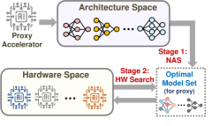
Figure 1. Overview of our semi-decoupled approach.

Proposition 3.1 ensures that in the presence of performance monotonicity, the same set $\mathcal{P}(h)$ of optimal architectures apply to all $h\in\mathcal{H}$. Thus, we can also simply use $\mathcal{P}$ to denote the set of optimal architectures, which are essentially shared by $h\in\mathcal{H}$. Note carefully that Proposition 3.1 does not mean that, given a specific pair of latency and energy constraints, we will have the same architecture $a^{*}(h_{1};L,E)=a^{*}(h_{2};L,E)$ for two hardware choices $h_{1},h_{2}\in\mathcal{H}$.

Nonetheless, once we have found $\mathcal{P}\subset\mathcal{A}$, there is no need to jointly search over the entire architecture-hardware space $\mathcal{A}\times\mathcal{H}$ any more. Instead, it is sufficient to merely search over the restricted architecture-hardware space $\mathcal{P}\times\mathcal{H}$. Importantly, the set $\mathcal{P}$ of optimal arachitectures is orders-of-magnitude smaller than the entire architecture space $\mathcal{A}$ (e.g., a few tens vs. $10^{18}$ in the DARTS architecture space (Liu et al., 2018)), thus significantly reducing the total hardware-software co-design cost without losing optimality.

1:  Input: Architecture space $\mathcal{A}$, hardware space $\mathcal{H}$, sample hardware $h_{0}\in\mathcal{H}$, and design constraints $L,E,H$ in Eqns. (2), (3), (4)

2:  Output: Optimal co-design $(a^{*},h^{*})$

3:  Initilization: Choose $K$ latency and energy constraints $(L_{k},E_{k})$ for $k=1,\cdots,K$, set $\mathcal{P}=\varnothing$, and randomly choose $(a^{*},h^{*})$;

4:  for $k=1,\cdots,K$ do

5:     For constraints $(L_{k},E_{k})$, run hardware-aware NAS to get optimal architecture $a_{k}^{*}(h_{0};L_{k},E_{k})$

6:     $\mathcal{P}=\mathcal{P}\bigcup\{a_{k}^{*}(h_{0};L_{k},E_{k})\}$;

7:  end for

8:  for each candidate hardware $h\in\mathcal{H}$ do

9:     if $HardwareResource(h)\leq H$ then

10:        Find optimal architecture $a^{*}(h)\in\mathcal{P}$ satisfying the latency and energy constraint $(L,E)$

11:        if $Accuracy(a^{*}(h))>Accuracy(a^{*})$ then

12:           $(a^{*},h^{*})\leftarrow(a^{*}(h),h)$

13:        end if

14:     end if

15:  end for

Algorithm 1 Semi-Decoupled Architecture-Accelerator Co-Design

Algorithm. Our semi-decoupled approach has two stages, as illustrated in Fig. 1 and summarized in Algorithm 1.

Stage 1: We randomly choose a sample accelerator $h_{0}\in\mathcal{H}$, which we refer to as the proxy accelerator, and run hardware-aware NAS for $K$ times to find a set of optimal architectures $\mathcal{P}=\mathcal{P}(h_{0})=(a_{1}^{*}(h_{0};L_{1},E_{1}),\cdots,a_{K}^{*}(h_{0};L_{K},E_{K}))$. Specifically, $\mathcal{P}$ is constructed by setting $K$ different latency and energy constraints and accordingly solving the inner NAS problem in Eqns. (7)—(9) for $K$ times. Thus, the search cost in Stage 1 is $\mathcal{O}(KM)$ where $M=|\mathcal{A}|$.

Stage 2: We search for the optimal accelerator $h^{*}\in\mathcal{H}$. Specifically, given each candidate $h\in\mathcal{H}$ (selected by, e.g., reinforcement learning or evolutionary search (Lu et al., 2019; Lin et al., 2021)), instead of searching over the entire architecture set $\mathcal{A}$, we obtain its corresponding optimal architecture $a^{*}(h)$ from the set $\mathcal{P}\subset\mathcal{A}$ constructed in Stage 1. Thus, the search cost in Stage 2 is $\mathcal{O}(KN)$ where $N=|\mathcal{H}|$.

3.3. Discussion

In practice, performance monotonicity may not be perfectly satisfied. Thus, the optimal architecture $a^{*}(h)$ corresponding to a candidate accelerator $h\in\mathcal{H}$ may not always strictly belong to the optimal architecture set $\mathcal{P}$ that is pre-constructed based on the proxy $h_{0}$. Nonetheless, by only searching over $\mathcal{P}$ for this candidate accelerator $h$, we can still find an architecture $a\in\mathcal{P}$ that is close-to-optimal. In fact, to speed up the NAS process and find competitive architectures, it is very common to use proxy/substitute metrics (such as accuracy predictor or the neural tangent kernel (Chen et al., 2021)) which only have SRCC of around 0.5–0.9 with the true performance. In our problem, we can also view the architectures’ latency and energy performance on the proxy accelerator $h_{0}$ as the substitute performance on other accelerator candidates. Therefore, given the good albeit not necessarily close-to-perfect performance monotonicity, the architectures optimized specifically for the proxy are also sufficiently competitive ones for other accelerator candidates.

In (Lu et al., 2021), scalable hardware-aware NAS is proposed by utilizing latency monotonicity on various devices. Without considering energy consumption, a high SRCC (¿0.9) for latency is needed to ensure that one proxy device’s optimal architectures are still close to optimal on another device. In our problem, such high SRCC values are not necessarily needed, because we consider both energy and latency — moderate SRCC values on two performance metrics are enough. This is reflected in both our experiments and prior studies (e.g., two proxy metrics having moderate SRCC values with the true accuracy can estimate the accuracy performance very well (Chen et al., 2021)).

In the highly unlikely event of very low SRCCs (e.g., 0.2) between the proxy and other accelerator candidates, we can enlarge $\mathcal{P}$ by adding some approximately optimal architectures near the Pareto boundary (for the chosen proxy), such that they can be competitive choices for other candidate accelerators. Alternatively, we could use a few proxy accelerators, each having good latency and energy monotonicity with a subspace of accelerator design, and jointly construct an expanded set $\mathcal{P}$ of optimal architectures in Stage 1. In any case, the set $\mathcal{P}$ is orders-of-magnitude smaller than the entire architecture space or accelerator space.

Summary. The essence of our semi-decoupled approach is to use a proxy $h_{0}$ to find a small set of optimal architectures that also includes the actual optimal or close-to-optimal architectures for different accelerator candidates, thus reducing the total co-design complexity without losing optimality. This is significantly different from a typical fully-decoupled approach that pre-searches for one architecture and then find the matching accelerator, and also has a sharp contrast with a fully-coupled co-design approach that jointly searches over the entire architecture-accelerator space. The comparison of different approaches is also summarized in Table 1. Importantly, our approach focuses on reducing the search space complexity, and can be integrated with any actual NAS (Stage 1) and accelerator exploration techniques (Stage 2).

4. Experiment Setup

We provide details of our experiment setup as follows.

Accelerator hardware space. We employ an open-source tool MAESTRO (Kwon et al., 2019) to simulate DNNs on the accelerator and measure inference metrics (e.g., latency and energy). MAESTRO supports a wide range of accelerators, including global shared scratchpad (i.e., L2 scratchapd), local PE scratchpad (i.e., L1 scratchpad), NoC, and a PE array organized into different hierarchies or dimensions.

DNN dataflow. Dataflow decides the DNN partitioning and scheduling strategies, which affects inference latency and energy performance. We consider three template dataflows: KC-P (motivated by NVDLA (NVIDIA, 2018)), YR-P (motivated by Eyeriss (Chen et al., 2016)), and X-P (weight-stationary). Exhibiting different characteristics (e.g., temporal reuse of input activation and filter in YR-P vs. spatial reuse of input activation in KC-P), these representative dataflows are all supported by MAESTRO (Kwon et al., 2019) and commonly used in SOTA hardware-software co-design (Yang et al., 2020).

Architecture space. We consider the following two spaces.

$\bullet$ NAS-Bench-301: It is a SOTA surrogate NAS benchmark built via deep ensembles and modeling uncertainty, which provides close-to-real predicted performances (i.e., accuracy and training time) of $10^{18}$ architectures on CIFAR-10 (Siems et al., 2020). We consider the DARTS space (Liu et al., 2018), where each architecture is a stack of 20 convolutional cells, and each cell consists of seven nodes.

$\bullet$ AlphaNet: It is a new family of architectures on ImageNet discovered by applying a generalized $\alpha$-divergence to supernet training (Wang et al., 2021a). Our search space is based on Table 7 of (Wang et al., 2021a), with a slight variation that the channel width is fixed as ”16, 16, 24, 32, 64, 112, 192, 216, 1792”, and depth, kernel size, expansion ratio of the first and last inverted residual blocks are fixed as ”1, 1”, ”3, 3”, ”1, 6”, respectively. For other searchable inverted residual blocks, the candidate depth, kernel size, and expansion ratio are ”2, 3, 4, 5, 6”, ”3, 5, 7”, and ”3, 4, 6”, respectively.

Search strategy. Our approach can be integrated with any NAS and hardware search strategies. Here, we consider exhaustive search over a pre-sampled subspace. Specifically, for the NAS-Bench-301, we first sample 10k models. Then, based on the accuracy given by NAS-Bench-301 and FLOPs of these 10k models, we select 1017 models, including the Pareto-optimal front (in terms of predicted accuracy and FLOPs) and some random architectures. Similarly, for the AlphaNet space, we first sample 10k models and then select 1046 models based on the predicted accuracy given by the released accuracy predictor (Facebook, 2021) and FLOPs. We consider a filtered space of 1k+ architectures (which include the Pareto-optimal ones out of the 10k sampled architectures), because using MAESTRO to measure the latency and energy of 10k models on thousands of different hardware-dataflow combinations is beyond our computational resource limit. For each of the three template dataflows, we sample 51 neural accelerators with different number of PEs, NoC bandwidth, and off-chip bandwidth per the MAESTRO document (of Technology, 2019). Specifically, the number of PEs can be chosen from “512, 256, 128, 64, 32, 16”, candidate NoC bandwidths are from “300, 400, 500, 600, 700, 800, 900, 1000”, and off-chip bandwidths are from “50, 100, 150, 200, 250, 275, 300, 325, 350”. Note that some of our sampled hardware-dataflow pairs are not supported when running with KC-P and YR-P dataflows on MAESTRO. Thus, the actual numbers of sampled accelerators (i.e., hardware-dataflow combinations) are 133 for NAS-Bench-301 and 132 for AlphaNet, respectively. We also consider layer-wise mixture of different dataflows (Section 5.3) to create 5000 different hardware-dataflow combinations.

5. Experimental Results

In this section, we present our experimental results. We show that strong performance monotonicity exists in the hardware design space, and highlight that our semi-decoupled approach can identify the optimal design at a much lower search complexity.

5.1. NAS-Bench-301

5.1.1. Performance monotonicity

We first validate that strong latency and energy performance monotonicity, quantified in SRCC, holds between different accelerators. The results are shown in Fig. 2. We see that, except for two accelerator choices that have SRCC less than 0.6 with others, all the other accelerators have almost perfect performance monotonicity with SRCC greater than 0.97. We also plot in Fig. 2(c) the cumulative distribution function (CDF) of the average SRCC values for all the sampled accelerators, where for each accelerator $h$ the “average” is over the SRCC values of all the accelerator pairs that include $h$. We see that the vast majority of the accelerators have average SRCC close to 1.

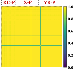
(a) Latency SRCC

(b) Energy SRCC

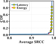
(c) CDF of SRCC

Figure 2. Performance monotonicity. We test 1017 models sampled in DARTS search space on 133 accelerators.

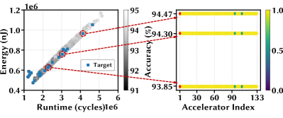
Figure 3. NAS-Bench-301. Left: The optimal models are marked in blue, and the grey scale indicates accuracy. Right: The accuracy of the model selected from the proxy’s optimal model set. We test each accelerator as a different proxy. We also select two proxy accelerators (indexes 95 and 107) that have the lowest SRCCs with the target, and show the detailed results in Table 2.

Accelerator Index SRCC Hardware Config. Model Performance Latency Energy PEs NoC Off-chip Dataflow Latency (cycles) Energy (nJ) Accuracy (%) 1 (target) 1 1 512 900 350 KC-P 2279256 626090 93.85 1-10[0.8pt/2pt] 107 0.556 0.567 64 400 250 YR-P 2279256 626090 93.85 1-10[0.8pt/2pt] 95 0.595 0.595 256 800 350 X-P 2279256 626090 93.85 1 (target) 1 1 512 900 350 KC-P 3027992 758928 94.30 1-10[0.8pt/2pt] 107 0.556 0.567 64 400 250 YR-P 3027992 758928 94.30 1-10[0.8pt/2pt] 95 0.595 0.595 256 800 350 X-P 3027992 758928 94.30 1 (target) 1 1 512 900 350 KC-P 4130699 964783 94.47 1-10[0.8pt/2pt] 107 0.556 0.567 64 400 250 YR-P 4130699 964783 94.47 1-10[0.8pt/2pt] 95 0.595 0.595 256 800 350 X-P 4130699 964783 94.47

Table 2. Hardware configuration of the target and two proxy accelerators, and performance metrics of the selected optimal models on each of them. “Accelerator Index” corresponds to the $x$-axis in right of Fig. 3, the models on the target accelerator correspond to the circled ones in left of Fig. 3, while the models on the two proxy accelerators correspond to the diamond marks located on the accelerator indexes. The architecture configuration of the target models is further illustrated in Table 5.1.1.

Target Model Model Architecture Normal Cell Config. Normal Cell Concat. Reduce Cell Config. Reduce Cell Concat. #1 (skip_connect, 0), (skip_connect, 1), (skip_connect, 0), (skip_connect, 2), (sep_conv_5x5, 0), (skip_connect, 1), (dil_conv_5x5, 4), (skip_connect, 2) [2, 3, 4, 5] (sep_conv_3x3, 1), (sep_conv_3x3, 0), (dil_conv_3x3, 2), (skip_connect, 0), (sep_conv_5x5, 2), (avg_pool_3x3, 0), (dil_conv_3x3, 3), (sep_conv_3x3, 1) [2, 3, 4, 5] 1-5[0.8pt/2pt] #2 (skip_connect, 0), (max_pool_3x3, 1), (sep_conv_3x3, 0), (skip_connect, 1), (skip_connect, 0), (’sep_conv_5x5, 3), (avg_pool_3x3, 4), (sep_conv_5x5, 1) [2, 3, 4, 5] (sep_conv_3x3, 1), (sep_conv_5x5, 0), (avg_pool_3x3, 0), (sep_conv_5x5, 1), (dil_conv_5x5, 3), (sep_conv_3x3, 2), (avg_pool_3x3, 4), (sep_conv_3x3, 0) [2, 3, 4, 5] 1-5[0.8pt/2pt] #3 (dil_conv_5x5, 0), (skip_connect, 1), (max_pool_3x3, 0), (max_pool_3x3, 2), (sep_conv_5x5, 0), (dil_conv_3x3, 3), (dil_conv_5x5, 3), (dil_conv_5x5, 4) [2, 3, 4, 5] (skip_connect, 0), (dil_conv_3x3, 1), (sep_conv_3x3, 1), (sep_conv_5x5, 2), (skip_connect, 1), (max_pool_3x3, 0), (skip_connect, 1), (sep_conv_5x5, 2) [2, 3, 4, 5] 1-5[0.8pt/2pt]

Table 3. Architecture configuration of the target models in Fig. 3. The first row (i.e., target model #1) corresponds to the leftmost circled model in Fig. 3, and second row corresponds to the middle circled model, etc. These are the configurations for each convolutional cell constructing a complete model, which is a stack of 20 cells. For detailed explanation of the operations in the DARTS search space, please refer to (Liu et al., 2018) and (Siems et al., 2020).

5.1.2. Effectiveness

To demonstrate the effectiveness, suppose that we have an optimal architecture-accelerator pair $(a^{*},h^{*})$ produced by the SOTA hardware-software co-design. We refer to the optimal accelerator as the “Target”. By using our approach, in Stage 1, we first randomly choose a non-target accelerator $h_{0}$ as our proxy, and run hardware-aware NAS on this proxy to obtain the set $\mathcal{P}$ of optimal architectures. Next, in Stage 2, we will search over the accelerator space, retrieve the corresponding architecture $a_{0}^{*}$ from $\mathcal{P}$ that best satisfies the latency and energy constraints, and keep the accelerator, whose corresponding architecture $a_{0}^{*}$ has the highest accuracy, as the optimal accelerator. Thus, we prove the effectiveness of our approach if the architecture $a_{0}^{*}\in\mathcal{P}$ corresponding to the optimal accelerator found in Stage 2 produces (approximately) the same accuracy as $a^{*}$ obtained using the SOTA co-design.

In our experiment, we consider a target optimal accelerator $h^{*}$ as follows: 512 PEs, NoC bandwidth constraint 900, off-chip bandwidth constraint 350, and KC-P dataflow. In Fig. 3, we plot all the optimal architectures under various latency and energy constraints. Then, we set three representative latency and energy consumption constraints, with their corresponding optimal models circled in red. Next, we test each of the other 132 accelerators as the proxy, and find the corresponding set $\mathcal{P}$, which includes about $20$ optimal architectures for that proxy. Then, we select the architecture from $\mathcal{P}$ whose latency and energy are closest to the design constraints on the target accelerator. We see that by using any of the 132 accelerators as the proxy, our approach can still find the optimal architecture that has (nearly) the same accuracy as that found by using SOTA hardware-software co-design. Importantly, even the proxy accelerator that has the lowest SRCC with the target can yield an competitive architecture with a good accuracy.

5.1.3. Total search cost

We now compare the total search cost incurred by exhaustive search over our sampled space. Using the coupled SOTA approach, the co-serach evaluates 133$*$1017$\approx$135K architecture-accelerator designs. In Stage 1 of our approach, we choose one proxy and evaluate 1017 architectures to obtain 20 optimal architectures for different latency and energy constraints. As we use exhaustive search, we do not need to run 20 times. In Stage 2, we evaluate the remaining 132 accelerators combined with the selected 20 architectures. Thus, the total search cost of our approach is 132$*$20+1017$\approx$3.7K, which is significantly less than 135K. While reinforcement learning or evolutionary search can improve the efficiency (especially on larger spaces), the order of the total cost remains the same. Moreover, when the architecture and accelerator spaces are larger, the relative advantage of our approach is even more significant.

Accelerator Index SRCC Hardware Config. Model Config. Latency Energy PEs NoC Off-chip Dataflow Latency (cycles) Energy (nJ) Accuracy (%) 1 (target) 1 1 512 900 350 KC-P 2061611 614779 69.60 1-11[0.8pt/2pt] 64 0.638 0.945 512 400 350 X-P 2061611 602782 69.58 1-11[0.8pt/2pt] 91 0.775 0.945 32 800 250 X-P 2046476 610891 69.60 1 (target) 1 1 512 900 350 KC-P 3367489 965462 71.18 1-11[0.8pt/2pt] 64 0.638 0.945 512 400 350 X-P 3367489 965462 71.18 1-11[0.8pt/2pt] 91 0.775 0.945 32 800 250 X-P 3367489 965462 71.18 1 (target) 1 1 512 900 350 KC-P 5923046 1858261 71.76 1-11[0.8pt/2pt] 64 0.638 0.945 512 400 350 X-P 5923046 1858261 71.76 1-11[0.8pt/2pt] 91 0.775 0.945 32 800 250 X-P 5923046 1858261 71.76

Table 4. Hardware configuration of the target and two proxy accelerators, and performance metrics of the selected optimal models on each of them. “Accelerator Index” corresponds to the $x$-axis in right of Fig. 5, models on the target accelerator correspond to the circled ones in left of Fig. 5, while the selected optimal models on proxy accelerators correspond to the diamond marks locating on the accelerator indexes. The architecture configuration of the target models is further illustrated in Table 5.1.3.

Target Model Model Architecture Resolution Width Kernel Size Expansion Ratio Depth #1 224 16, 16, 24, 32, 64, 112, 192, 216, 1792 3, 3, 3, 3, 3, 3, 3 1, 4, 4, 6, 6, 5, 6 1, 3, 4, 3, 3, 3, 1 1-6[0.8pt/2pt] #2 288 16, 16, 24, 32, 64, 112, 192, 216, 1792 3, 3, 3, 3, 3, 7, 3 1, 4, 4, 5, 4, 5, 6 1, 3, 3, 3, 4, 4, 1 1-6[0.8pt/2pt] #3 288 16, 16, 24, 32, 64, 112, 192, 216, 1792 3, 3, 5, 7, 7, 7, 3 1, 6, 6, 6, 5, 5, 6 1, 6, 6, 3, 6, 6, 1 1-6[0.8pt/2pt]

Table 5. Architecture configuration of target models in Fig. 5. The first row (i.e., target model #1) corresponds to the leftmost circled model in Fig. 5, and second row corresponds to the middle circled model, etc. For detailed explanation of the operations in AlphaNet search space, please refer to (Wang et al., 2021b).

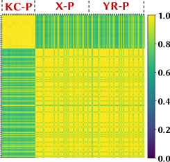
(a) SRCC of Latency

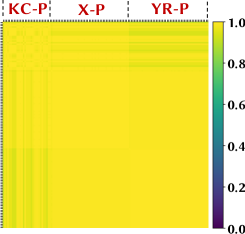
(b) SRCC of Energy Consumption

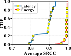
(c) CDF of SRCC

Figure 4. Performance monotonicity. We test 1046 models sampled in AlphaNet search space on 132 accelerators.

5.2. AlphaNet

We now turn to the AlphaNet architecture space, and show the results in Fig. 4 and Fig. 5. While the SRCC values are lower than those in the NAS-Bench-301 case, they are still generally very high (e.g., mostly ¿0.9). Crucially, as shown in Fig. 5, our approach can successfully find an architecture that has (almost) the same accuracy as that obtained by using the SOTA coupled approach.

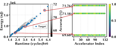
Figure 5. AlphaNet. Left: The optimal models are marked in blue, and the grey scale indicates accuracy. Right: The accuracy of the model selected from the proxy’s optimal model set. We test each accelerator as a different proxy. We select two proxy accelerators (indexes 64 and 91) and show the detailed results in Table 4.

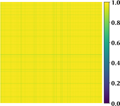
(a) Latency SRCC

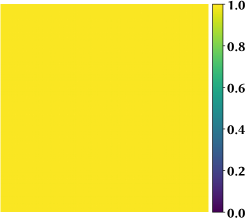
(b) Energy SRCC

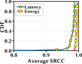
(c) CDF of SRCC

Figure 6. Performance monotonicity. We test 1017 models sampled in DARTS on 5000 accelerators with layer-wise mixed dataflows.

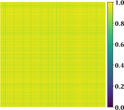
(a) Latency SRCC

(b) Energy SRCC

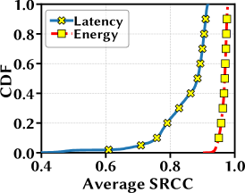
(c) CDF of SRCC

Figure 7. Performance monotonicity. We test 1046 models sampled in AlphaNet on 5000 accelerators with layer-wise mixed dataflows.

5.3. Layer-wise Mixed Dataflow

Ideally, each layer of a DNN model can be switched between accelerator hardware and dataflows to search for the best combination (especially in the multi-accelerator design case) (Yang et al., 2020). To account for this, we divide each model into 22 parts: first and last convolutional layer, and evenly into 20 groups for all intermediate layers. For each part, it can be executed on any of our 51 sampled hardware configurations following any dataflow. We sample 5000 different mixtures for our models in NAS-Bench-301 and AlphaNet spaces, and report the SRCC results in Fig. 6 and 7, respectively. The results confirm again that strong performance monotonicity exists and ensures the effectiveness of our approach. We omit the optimal accuracy results due to the lack of space, while noting that they are similar to Figs. 3 and 5.

6. Related Work

NAS and accelerator design. Hardware-aware NAS has been actively studied to incorporate characteristics of target device and automate the design of optimal architectures subject to latency and/or energy constraints (Lu et al., 2019; Li et al., 2021; Yang et al., 2018; Bender et al., 2020; Chu et al., 2021; Ren et al., 2020; Tan et al., 2019; Wu et al., 2019). These studies do not explore the hardware design space. A recent NAS study (Lu et al., 2021) explores latency monotonicity to scale up NAS across different devices, but it only considers latency constraints and, like other NAS studies, does explore the hardware design space. In parallel, there have also been studies on automating the design of accelerators for DNNs (Xu et al., 2020). But, NAS and accelerator design have been traditionally studied in a siloed manner, resulting in sub-optimal designs.

Architecture-accelerator co-design. The studies on jointly optimizing architectures and accelerators have been quickly expanding. For example, (Yang et al., 2020) jointly optimizes neural architectures and ASIC accelerators using reinforcement learning, (Jiang et al., 2020b) performs a two-level (fast and slow) hardware exploration for each candidate neural architecture, (Jiang et al., 2020a) adopts a set of manually selected models as the hot start state for acceleration exploration, and (Lin et al., 2021) co-designs neural architecture, hardware configuration and dataflow, and employs evolutionary search to reduce the search cost. These studies primarily focus on improving the search efficiency given a certain search space. By contrast, we use a principled approach to reducing the total search space, without losing optimality.

7. Conclusion

In this paper, we reduce the total hardware-software co-design cost by semi-decoupling NAS from accelerator design. Concretely, we demonstrate latency and energy monotonicity among different accelerators, and use just one proxy accelerator’s optimal architecture set to avoid searching over the entire architecture space. Compared to the SOTA co-designs, our approach can reduce the total design complexity by orders of magnitude, without losing optimality. Finally, we validate our approach via experiments on two search spaces — NAS-Bench-301 and AlphaNet.

Acknowledgement

B. Lu and S. Ren were supported in part by the U.S. National Science Foundation under grant CNS-1910208. Z. Yan and S. Shi were supported in part by the U.S. National Science Foundation under grant CNS-1822099.

References

- (1)
- Ahn et al. (2020) Byung Hoon Ahn, Prannoy Pilligundla, Amir Yazdanbakhsh, and Hadi Esmaeilzadeh. 2020. Chameleon: Adaptive Code Optimization for Expedited Deep Neural Network Compilation. In ICLR.
- Akoglu (2018) Haldun Akoglu. 2018. User’s guide to correlation coefficients. Turkish journal of emergency medicine (2018).
- Amazon (2019) Amazon. 2019. Amazon EC2 F1 Instances. https://aws.amazon.com/ec2/instance-types/f1/.
- Bender et al. (2020) Gabriel Bender, Hanxiao Liu, Bo Chen, Grace Chu, Shuyang Cheng, Pieter-Jan Kindermans, and Quoc V Le. 2020. Can weight sharing outperform random architecture search? an investigation with tunas. In CVPR.
- Cai et al. (2019) Han Cai, Chuang Gan, and Song Han. 2019. Once for All: Train One Network and Specialize it for Efficient Deployment. In ICLR.
- Chen et al. (2021) Wuyang Chen, Xinyu Gong, and Zhangyang Wang. 2021. Neural Architecture Search on ImageNet in Four GPU Hours: A Theoretically Inspired Perspective. In ICLR. https://openreview.net/forum?id=Cnon5ezMHtu
- Chen et al. (2016) Yu-Hsin Chen, Joel Emer, and Vivienne Sze. 2016. Eyeriss: A spatial architecture for energy-efficient dataflow for convolutional neural networks. ACM SIGARCH Computer Architecture News (2016).
- Chu et al. (2021) Grace Chu, Okan Arikan, Gabriel Bender, Weijun Wang, Achille Brighton, Pieter-Jan Kindermans, Hanxiao Liu, Berkin Akin, Suyog Gupta, and Andrew Howard. 2021. Discovering multi-hardware mobile models via architecture search. In CVPR.
- Dai et al. (2019) Xiaoliang Dai, Peizhao Zhang, Bichen Wu, Hongxu Yin, Fei Sun, Yanghan Wang, Marat Dukhan, Yunqing Hu, Yiming Wu, Yangqing Jia, et al. 2019. ChamNet: Towards Efficient Network Design Through Platform-Aware Model Adaptation. In CVPR.
- Facebook (2021) Facebook. 2021. AlphaNet: Improved Training of Supernet with Alpha-Divergence. https://github.com/facebookresearch/AlphaNet.
- Jiang et al. (2019) Weiwen Jiang, Edwin H.-M. Sha, Xinyi Zhang, Lei Yang, Qingfeng Zhuge, Yiyu Shi, and Jingtong Hu. 2019. Achieving Super-Linear Speedup Across Multi-FPGA for Real-Time DNN Inference. ACM Trans. Embed. Comput. Syst. 18, 5s, Article 67 (Oct. 2019), 67:1–67:23 pages.
- Jiang et al. (2020a) Weiwen Jiang, Lei Yang, Sakyasingha Dasgupta, Jingtong Hu, and Yiyu Shi. 2020a. Standing on the Shoulders of giants: Hardware and neural architecture co-search with hot start. IEEE Transactions on Computer-Aided Design of Integrated CIrcuits and Systems (2020).
- Jiang et al. (2020b) Weiwen Jiang, Lei Yang, Edwin Hsing-Mean Sha, Qingfeng Zhuge, Shouzhen Gu, Sakyasingha Dasgupta, Yiyu Shi, and Jingtong Hu. 2020b. Hardware/software co-exploration of neural architectures. IEEE Transactions on Computer-Aided Design of Integrated Circuits and Systems (2020).
- Kwon et al. (2019) Hyoukjun Kwon, Prasanth Chatarasi, Michael Pellauer, Angshuman Parashar, Vivek Sarkar, and Tushar Krishna. 2019. Understanding Reuse, Performance, and Hardware Cost of DNN Dataflow: A Data-Centric Approach. In MICRO.
- Li et al. (2021) Chaojian Li, Zhongzhi Yu, Yonggan Fu, Yongan Zhang, Yang Zhao, Haoran You, Qixuan Yu, Yue Wang, Cong Hao, and Yingyan Lin. 2021. HW-NAS-Bench: Hardware-Aware Neural Architecture Search Benchmark. In ICLR. https://openreview.net/forum?id=_0kaDkv3dVf
- Lin et al. (2021) Yujun Lin, Mengtian Yang, and Song Han. 2021. NAAS: Neural Accelerator Architecture Search. In 2021 58th ACM/ESDA/IEEE Design Automation Conference (DAC).
- Liu et al. (2018) Hanxiao Liu, Karen Simonyan, and Yiming Yang. 2018. Darts: Differentiable architecture search. arXiv preprint arXiv:1806.09055 (2018).
- Lu et al. (2021) Bingqian Lu, Jianyi Yang, Weiwen Jiang, Yiyu Shi, and Shaolei Ren. 2021. One Proxy Device Is Enough for Hardware-Aware Neural Architecture Search. Proc. ACM Meas. Anal. Comput. Syst. 5, 3, Article 34 (dec 2021), 34 pages.
- Lu et al. (2019) Qing Lu, Weiwen Jiang, Xiaowei Xu, Yiyu Shi, and Jingtong Hu. 2019. On Neural Architecture Search for Resource-Constrained Hardware Platforms. In ICCAD.
- Microsoft (2019) Microsoft. 2019. Microsoft Project Brainwave. https://www.microsoft.com/en-us/research/project/project-brainwave/.
- NVIDIA (2018) NVIDIA. 2018. NVDLA Deep Learning Accelerator. http://nvdla.org.
- of Technology (2019) Georgia Institute of Technology. 2019. MAESTRO’s documentation. http://maestro.ece.gatech.edu/docs/build/html/examples/running_maestro.html.
- Ren et al. (2020) Pengzhen Ren, Yun Xiao, Xiaojun Chang, Po-Yao Huang, Zhihui Li, Xiaojiang Chen, and Xin Wang. 2020. A comprehensive survey of neural architecture search: Challenges and solutions. arXiv preprint arXiv:2006.02903 (2020).
- Siems et al. (2020) Julien Siems, Lucas Zimmer, Arber Zela, Jovita Lukasik, Margret Keuper, and Frank Hutter. 2020. NAS-Bench-301 and the Case for Surrogate Benchmarks for Neural Architecture Search. arXiv preprint arXiv:2008.09777 (2020).
- Tan et al. (2019) Mingxing Tan, Bo Chen, Ruoming Pang, Vijay Vasudevan, Mark Sandler, Andrew Howard, and Quoc V. Le. 2019. MnasNet: Platform-Aware Neural Architecture Search for Mobile. In CVPR.
- Tan and Le (2019) Mingxing Tan and Quoc Le. 2019. EfficientNet: Rethinking Model Scaling for Convolutional Neural Networks. In ICML. http://proceedings.mlr.press/v97/tan19a.html
- Wang et al. (2021a) Dilin Wang, Chengyue Gong, Meng Li, Qiang Liu, and Vikas Chandra. 2021a. AlphaNet: Improved Training of Supernet with Alpha-Divergence. arXiv preprint arXiv:2102.07954 (2021).
- Wang et al. (2021b) Dilin Wang, Meng Li, Chengyue Gong, and Vikas Chandra. 2021b. Attentivenas: Improving neural architecture search via attentive sampling. In CVPR.
- Wang et al. (2020) Tianzhe Wang, Kuan Wang, Han Cai, Ji Lin, Zhijian Liu, Hanrui Wang, Yujun Lin, and Song Han. 2020. APQ: Joint Search for Network Architecture, Pruning and Quantization Policy. In CVPR.
- Wen et al. (2019) Wei Wen, Hanxiao Liu, Hai Li, Yiran Chen, Gabriel Bender, and Pieter-Jan Kindermans. 2019. Neural Predictor for Neural Architecture Search. arXiv preprint arXiv:1912.00848 (2019).
- Williams et al. (2009) Samuel Williams, Andrew Waterman, and David Patterson. 2009. Roofline: An Insightful Visual Performance Model for Multicore Architectures. Commun. ACM 52, 4 (apr 2009), 65–76. https://doi.org/10.1145/1498765.1498785
- Wu et al. (2019) Bichen Wu, Xiaoliang Dai, Peizhao Zhang, Yanghan Wang, Fei Sun, Yiming Wu, Yuandong Tian, Peter Vajda, Yangqing Jia, and Kurt Keutzer. 2019. FBNet: Hardware-Aware Efficient ConvNet Design via Differentiable Neural Architecture Search. In CVPR.
- Xu et al. (2020) Pengfei Xu, Xiaofan Zhang, Cong Hao, Yang Zhao, Yongan Zhang, Yue Wang, Chaojian Li, Zetong Guan, Deming Chen, and Yingyan Lin. 2020. AutoDNNchip: An Automated DNN Chip Predictor and Builder for Both FPGAs and ASICs. In FPGA.
- Yang et al. (2020) Lei Yang, Zheyu Yan, Meng Li, Hyoukjun Kwon, Liangzhen Lai, Tushar Krishna, Vikas Chandra, Weiwen Jiang, and Yiyu Shi. 2020. Co-exploration of neural architectures and heterogeneous asic accelerator designs targeting multiple tasks. In DAC.
- Yang et al. (2018) Tien-Ju Yang, Andrew Howard, Bo Chen, Xiao Zhang, Alec Go, Mark Sandler, Vivienne Sze, and Hartwig Adam. 2018. NetAdapt: Platform-Aware Neural Network Adaptation for Mobile Applications. In ECCV.
- Zoph and Le (2016) Barret Zoph and Quoc V Le. 2016. Neural architecture search with reinforcement learning. arXiv preprint arXiv:1611.01578 (2016).