Self-supervised Semantic Segmentation Grounded in Visual Concepts

Appendix A Supplementary Material

In this supplementary material, we include:

• ablation study regarding hyper-parameters;

• per-class results on Pascal VOC 2012 validation set;

• visualization of the global concepts;

• visualization of the pixel embeddings and the instance masks on DAVIS-2017 validation set.

A.1 Ablation Study

We conduct experiments for the ablation study to understand how the hyper-parameters affect the performance of our method, including the weights of the losses, the number of global concepts, the commitment constant $\beta$, and the memory bank size.

Weights of the losses.

We fix $\lambda_{s}$ to 1 and vary $\lambda_{v}$ and $\lambda_{c}$ to perform the ablation experiments. The results are shown in Table 1. We find that our model performs well (i.e., outperforms the model that only uses local concepts by a large margin) when $\lambda_{v}$ is greater than 1 and $\lambda_{c}$ is smaller than 2.

$\lambda_{v}$	$\lambda_{c}$	mIoU	mIoU
		($k$-means)	(LC)
0.5	1	61.58	62.86
1	1	62.08	63.06
1.5	1	62.22	63.22
2	1	62.56	63.47
2.5	1	62.62	63.83
3	1	62.27	63.47

$\lambda_{v}$	$\lambda_{c}$	mIoU	mIoU
		($k$-means)	(LC)
2	0.5	62.10	62.88
2	1	62.56	63.47
2	1.5	61.98	64.04
2	2	61.62	63.31
2	2.5	61.07	63.41
2	3	60.97	63.21

Table 1: Experiments on different weights of loss terms.

Number of global concepts.

We train our model on Pascal VOC 2012 train_aug set with 32, 64, 128, 256, 512, and 1024 global concepts. We test the trained models with $k$-means clustering and nearest neighbors retrieval on the validation set of Pascal VOC 2012. The experiment results are shown in Table 2. We find that the model does not perform well if the number of global concepts is smaller than 128. The reason could be that the model aggregates image segments with different semantic meanings into the same global concept as there are only a small number of global concepts.

Num of Global Concepts	mIoU
32	60.90
64	61.45
128	61.85
256	62.07
512	62.56
1024	62.20

Table 2: Model’s performance with respect to the number of global concepts. To obtain a good performance, there should be enough global concepts (e.g., more than 256 concepts).

Commitment constant $\beta$.

The commitment constant $\beta$ is used to control how much the global concepts affect the pixel embeddings. Higher $\beta$ means the pixel embeddings are more concentrate around the learned global concepts. We train our model with different values of $\beta$ on Pascal VOC 2012 train_aug set and test the trained models with $k$-means clustering and nearest neighbors retrieval on the validation set of Pascal VOC 2012. We can see that the model performs better if the commitment constant $\beta$ is greater than 0.3, which indicates that regularizing the pixel embeddings based on the global concepts can benefit the model’s performance. Note that although the choice of the hyper-parameters could affect the model’s performance, our model still outperforms previous work by more than 5% with the hyper-parameters used in the ablation study.

Commitment Constant $\beta$	mIoU
0.1	61.64
0.2	61.46
0.3	62.03
0.4	62.34
0.5	62.56
0.6	62.29
0.7	62.10

Table 3: Model’s performance with respect to the commitment constant $\beta$. The model performs better if the commitment constant $\beta$ is greater than 0.3, which means regularizing the pixel embeddings based on the global concepts can benefit the model’s performance.

Method	Pseudo Seg.	Background	Aero	Bike	Bird	Boat	Bottle	Bus	Car	Cat	Chair	Cow	Table	Dog	Horse	MBike	Person	Plant	Sheep	Sofa	Train	TV	mIoU
SegSort	HED	88.30	67.52	29.34	67.82	39.88	49.45	61.94	64.88	74.43	5.85	26.41	16.33	67.03	44.06	63.28	71.21	13.28	52.15	22.65	58.15	48.63	49.17
MaskContrast	Unsup. Sal.	84.27	68.32	23.26	49.78	42.44	54.99	82.21	67.02	62.57	7.15	50.38	33.96	59.29	49.66	60.12	52.37	20.63	55.47	21.28	63.33	34.64	49.67
MaskContrast	Sup. Sal.	86.00	62.99	23.63	56.08	45.28	61.31	74.68	71.33	64.89	6.70	46.55	35.21	63.80	46.67	58.83	58.03	32.53	60.07	29.69	67.17	47.95	52.35
Ours	HED	91.02	80.47	33.93	80.42	59.93	67.15	81.94	74.00	83.25	19.00	52.45	50.85	76.12	54.41	66.89	75.63	37.97	65.57	34.47	70.07	58.34	62.56

Table 4: Per-class results on Pascal VOC 2012 validation set using $k$-means clustering and nearest neighbors retrieval. Our method outperforms previous work consistently.

Method	Pseudo Seg.	Background	Aero	Bike	Bird	Boat	Bottle	Bus	Car	Cat	Chair	Cow	Table	Dog	Horse	MBike	Person	Plant	Sheep	Sofa	Train	TV	mIoU
SegSort	HED	89.82	74.26	35.34	74.87	54.60	63.75	71.30	68.07	78.57	18.01	53.91	30.15	70.54	54.01	68.43	73.59	41.22	62.41	25.45	65.13	62.40	58.85
MaskContrast	Unsup. Sal.	90.10	85.38	34.22	76.46	63.57	67.93	84.22	75.00	78.59	14.20	66.29	40.88	73.55	62.00	71.86	70.48	30.02	71.44	30.63	72.22	47.60	62.22
MaskContrast	Sup. Sal.	91.26	87.23	32.98	79.56	65.68	68.13	84.48	77.47	81.31	20.59	68.22	44.82	75.57	65.11	72.28	73.90	40.87	76.03	30.29	76.48	54.48	65.08
Ours	HED	90.73	78.06	35.28	80.78	56.09	68.04	81.80	73.73	85.02	24.75	62.41	42.07	76.92	61.04	67.15	76.85	41.83	67.73	29.25	71.95	61.44	63.47

Table 5: Per-class results on Pascal VOC 2012 validation set using linear classification. Our method outperforms most of the previous work except MaskContrast with a salience estimator trained on a large number of annotated images.

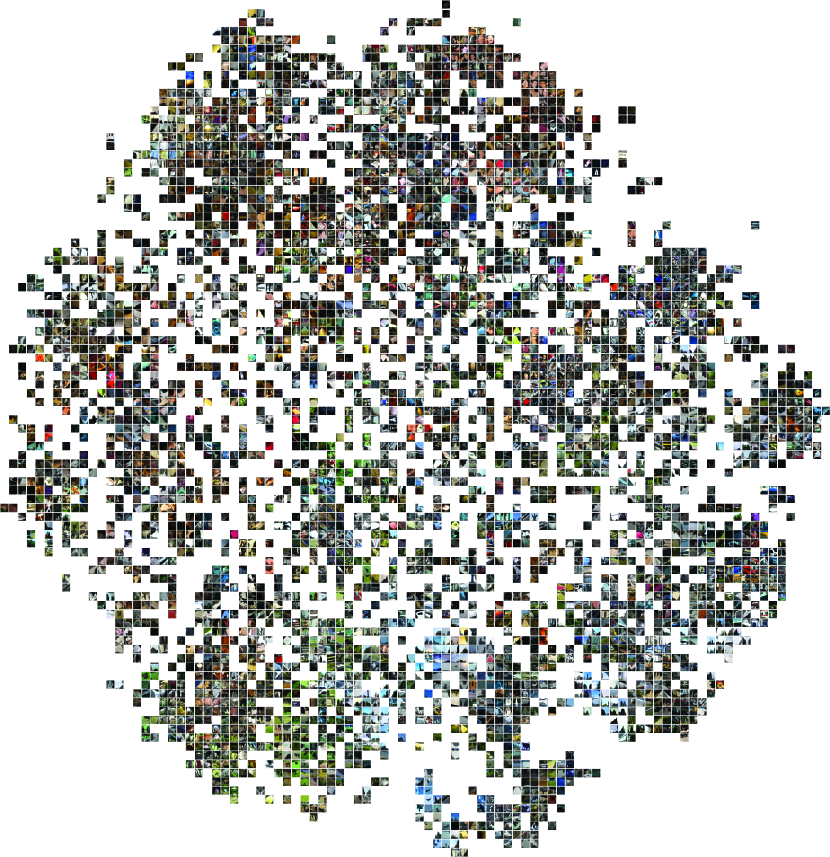
Figure 1: t-SNE visualization of image segments sampled from global concepts based on the segments’ latent representation. Best viewed with zoom-in.

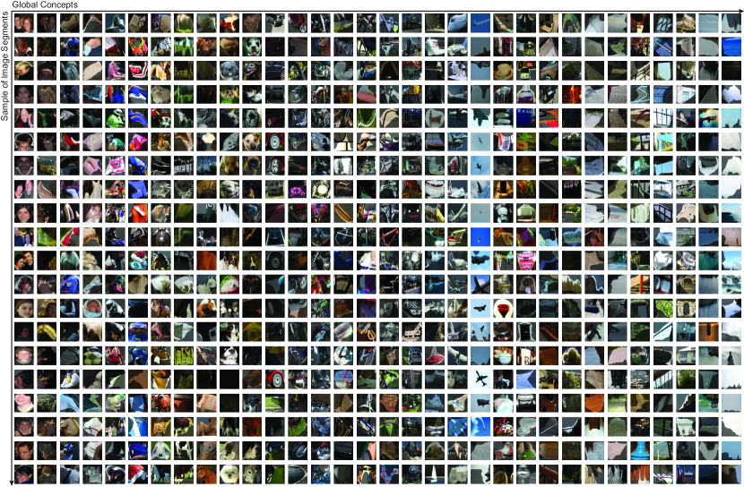
Figure 2: Image segments sampled from 32 concepts (one concept per column). Fine-grained visual concepts representing different object parts or specific scenarios can be extracted from the data using our method.

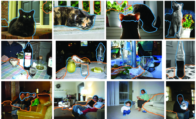
Figure 3: Image retrieval based on the visual concepts. By associating the learned visual concepts, we can create sophisticated scenarios for image retrieval, such as cat next to plants, bottles on a table, or people sitting on a sofa.

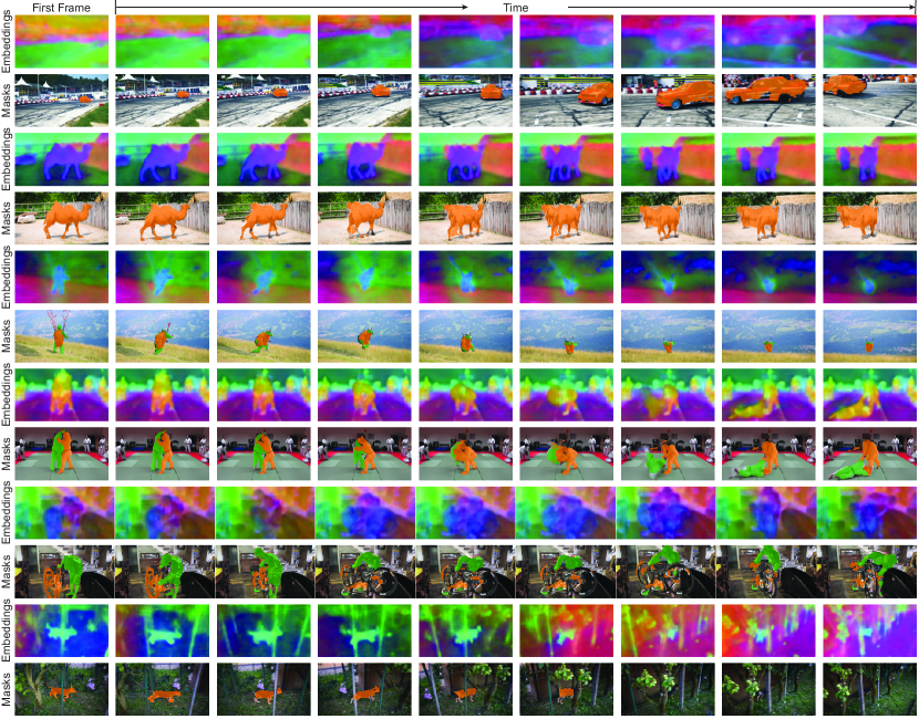
Figure 4: Visualization of the pixel embeddings and instance masks produced by our method on DAVIS-2017 validation set.

Memory bank size.

By training our model with different memory bank size, we find that our method performs better with a bigger memory bank (e.g., mIoUs are 59.96, 61.62, and 62.56 for memory bank of 0, 1, and 2 batches, respectively). Similar findings were also discovered in the previous work (Hwang et al. 2019). In the main paper, we use a memory bank of 2 batches (8 images per batch) for all the baselines except hierarchical grouping (Zhang and Maire 2020), which uses a much bigger batch size (i.e., 70 images per batch).

A.2 Per-class Results on Pascal VOC 2012

Table 4 shows per-class results on Pascal VOC 2012 validation set using $k$-means clustering and nearest neighbors retrieval. Our method outperforms previous work consistently. Especially on class aero, bird, chair, and table, our method outperforms previous work by more than 10% on IoU.

Table 5 shows per-class results on Pascal VOC 2012 validation set using linear classification. Our method outperforms most of the previous work on most of the classes. The only exception is MaskContrast with a salience estimator trained on a large number of annotated images, which outperforms our method on approximately 2/3 of the classes.

A.3 Visualization of the Concepts

We first use t-SNE to visualize the image segments extracted from Pascal VOC 2012 validation set based on the global concepts. We project the latent representation of the image segments to a 2-dimensional space and use the 2-dimensional embeddings to layout the image segments. The visualization is shown in Figure 1. We observe that the image segments form clear visual groups in the latent space. For example, human faces are clustered on the top right. Buses are placed on the right side. Farm animals and grasslands are placed on the bottom left.

We then visualize the learned visual concepts by sampling a set of image segments from each concept as shown in Figure 2. We can see that our method can extract fine-grained visual concepts representing different object parts (e.g., human faces, car tires, and animal feet) and sub-classes (e.g., babies, cups, and fences). In addition, our method can learn concepts for specific scenarios, such as a human wearing a helmet or an airplane flying in the sky.

By associating the learned visual concepts, we can create sophisticated scenarios for image retrieval and data analysis. For example, in Figure 3, we use the relationships (e.g., relative positions) between different concepts to retrieve images that contain cat next to plants, bottles on a table, or people sitting on a sofa.

A.4 Visualization of Pixel Embeddings on DAVIS-2017

Figure 4 visualizes the pixel embeddings and the instance masks produced by our method on DAVIS-2017 validation set. For each video, we visualize the results till late frames. We find that our method can produce relatively consistent embeddings for long sequences of video frames and various types of objects such as cars, humans, and animals. Meanwhile, our method may lose track of objects that are heavily occluded such as the last row in Figure 4.