A Stitch in Time Saves Nine:
A Train-Time Regularizing Loss for Improved Neural Network Calibration

Abstract

Deep Neural Networks (dnns) are known to make overconfident mistakes, which makes their use problematic in safety-critical applications. State-of-the-art (sota) calibration techniques improve on the confidence of predicted labels alone, and leave the confidence of non-max classes (e.g. top-2, top-5) uncalibrated. Such calibration is not suitable for label refinement using post-processing. Further, most sota techniques learn a few hyper-parameters post-hoc, leaving out the scope for image, or pixel specific calibration. This makes them unsuitable for calibration under domain shift, or for dense prediction tasks like semantic segmentation. In this paper, we argue for intervening at the train time itself, so as to directly produce calibrated dnn models. We propose a novel auxiliary loss function: Multi-class Difference in Confidence and Accuracy (mdca), to achieve the same. mdca can be used in conjunction with other application/task specific loss functions. We show that training with mdca leads to better calibrated models in terms of Expected Calibration Error (ece), and Static Calibration Error (sce) on image classification, and segmentation tasks. We report ece (sce) score of 0.72 (1.60) on the cifar 100 dataset, in comparison to 1.90 (1.71) by the sota. Under domain shift, a ResNet-18 model trained on pacs dataset using mdca gives a average ece (sce) score of 19.7 (9.7) across all domains, compared to 24.2 (11.8) by the sota. For segmentation task, we report a $2\times$ reduction in calibration error on pascal-voc dataset in comparison to Focal Loss [34]. Finally, mdca training improves calibration even on imbalanced data, and for natural language classification tasks.

1 Introduction

Deep Neural Networks (dnns) have shown promising results for various pattern recognition tasks in recent years. In a classification setting, with input $\mathbf{x}\in\mathcal{X}$, and label $y\in{\mathcal{Y}}=\{1,\ldots,K\}$, a dnn typically outputs a confidence score vector $\mathbf{s}\in\mathbb{R}^{K}$. The vector, $\mathbf{s}$, is also a valid probability vector, and each element of $\mathbf{s}$ is assumed to be the predicted confidence for the corresponding label. It has been shown in recent years that the confidence vector, $\mathbf{s}$, output by a dnn is often poorly calibrated [14, 38]. That is:

$$\mathbb{P}\Big{(}\widehat{y}=y^{*}~{}\big{|}~{}\mathbf{s}[\widehat{y}]\Big{)}~{}\neq~{}\mathbf{s}[\widehat{y}],$$ (1)

where $\widehat{y}$, and $y^{*}$ are the predicted, and true label respectively for a sample. E.g. if a dnn predicts a class “truck” for an image with score 0.7, then a network is calibrated, if the probability that the image actually contains a truck is 0.7. If the probability is lower, a network is said to be over-confident, and under-confident if probability is higher. For a pixel-wise prediction task like semantic segmentation, we would like to calibrate prediction for each pixel. Similarly, we would like calibration to hold not only for the predicted label, i.e. $\widehat{y}=\underset{y\in{\mathcal{Y}}}{\operatorname{arg}\,\operatorname{max}}\;\mathbf{s}[y]$, but for the whole vector $\mathbf{s}$ (all labels), i.e., $\forall y\in{\mathcal{Y}}$.

One of the main reasons for the miscalibration is the specific training regimen used. Most modern dnns, when trained for classification in a supervised learning setting, are trained using one-hot encoding that have all the probability mass centered in one class; the training labels are thus zero-entropy signals that admit no uncertainty about the input [51]. The dnn is thus trained to become overconfident. Besides creating a general distrust in the model predictions, the miscalibration is especially problematic in safety critical applications, such as self-driving cars [13], legal research [54] and healthcare [49, 10], where giving the correct confidence for a predicted label is as important as the correct label prediction itself.

Researchers have tried to address miscalibration by learning a post-hoc transformation of the output vector so that the confidence of the predicted label matches with the likelihood of the label for the sample [18, 16]. Since such techniques focus on the predicted label only, they could end up calibrating only the label which has maximum confidence for each sample. Hence, in a multi-class setting, the labels with non-maximal confidence scores remain uncalibrated. This makes any post-processing for label refinement, such as posterior inference using MRF-MAP [4], ineffective.

In this paper we argue for the calibration at the train-time. Unlike post-hoc calibration techniques that use limited parameters, a train time strategy allows exploiting millions of learnable parameters of DNN itself, thus providing a flexible learning more suited to image and pixel specific transformation for model calibration. Our experiments under domain shift, and for a dense predict task (semantic segmentation) shows the strength of the approach.

Armed with the above insight, we propose a novel auxiliary loss function: Multi-class Difference in Confidence and Accuracy (mdca). The proposed loss function is designed to be used during the training stage in conjunction with other application specific loss functions, and overcomes the non-differentiablity of the loss functions proposed in earlier methods. Though we do not advocate it, the proposed technique is complimentary to the post-hoc techniques which may still be used after the training, if there is a separate hold-out dataset available for exploitation. Since ours is a train time calibration approach, it implies good regularization for the predictions. We show that models trained using our loss function remain calibrated even under domain shift.

Contributions: We make the following key contributions: (1) A trainable dnn calibration method with inclusion of a novel auxiliary loss function, termed mdca, that takes into account the entire confidence vector in a multi-class setting. Our loss function is differentiable and can be used in conjunction with any existing loss term. We show experiments with Cross-Entropy, Label Smoothing [40], and Focal Loss [34]. (2) Our approach is on par with post-hoc methods [24, 14] without the need for hold-out set making the deployment more practical (See Tab. 6). (3) Our loss function is a powerful regularizer, maintaining calibration even under domain/dataset drift and dataset imbalance which We demonstrate on pacs [31], Rotated MNIST [30] and imbalanced cifar 10 datasets. (4) Although the focus is primarily on image classification, our experiments on multi-class semantic segmentation show that our technique outperforms ts based calibration, and Focal Loss [34]. We also show the effectiveness of our approach on natural language classification task on 20Newsgroup dataset [28].

2 Related Work

Techniques for calibrating dnns can be broadly classified into train-time calibration, post-hoc calibration, and calibration through Out-Of-Distribution (ood). Train-time calibration integrate model calibration during the training procedure while a post-hoc calibration method utilizes a hold-out set to tune the calibration measures. On the other hand,learning to reject ood samples (at train-time or post-hoc) mitigates overconfidence and thus, calibrates dnns.

Train-Time Calibration: One of the earliest train-time methods proposes Brier Score for the calibrating binary probabilistic forecast [2]. [14] show models trained with Negative-Log-Likelihood (nll) tend to be over-confident and empirically show a disconnect between nll and accuracy. Specifically, the overconfident scores necessitates re-calibration. A common calibration approach is to use additional loss terms other than the nll loss: [47] use entropy as a regularization term whereas Müller et al.[40] propose Label Smoothing (ls) [50] on soft-targets which aids in improving calibration. Recently, [39] showed that focal loss [34] can implicitly calibrate dnns by reducing the KL-divergence between predicted and target distribution whilst increasing the entropy of the predicted distribution, thereby preventing the model from becoming overconfident. Liang et al.[32] have proposed an auxiliary loss term, dca, which is added with Cross-Entropy to help calibrate the model. The dca term penalizes the model when the cross-entropy loss is reduced, but the accuracy remains the same, i.e., when the over-fitting occurs. [27] propose to use mmce, an auxiliary loss term for calibration, computed using a reproducing kernel in a Hilbert space [12]. Maroñas et al.[35] analyse MixUp [55] data augmentation for calibrating DNNs and conclude Mixup does not necessarily improve calibration.

Post-Hoc Calibration: Post-hoc calibration techniques calibrate a model using a hold-out training set, which is usually the validation set. Temperature scaling (ts) smoothes the logits to calibrate a dnn. Specifically, ts is a variant of Platt scaling [48] that works by dividing the logits by a scalar $T>0$, learnt on a hold-out training set, prior to taking a softmax. The downside of using ts during calibration is reduction in confidence of every prediction, including the correct one. A more general version of ts transforms the logits using a matrix scaling. The matrix $M$ is learnt using the hold-out set similar to ts. Dirichlet calibration (dc) uses Dirichlet distributions to extend the Beta-calibration [25] method for binary classification to a multi-class one. dc is easy to implement as an extra layer in a neural network on log-transformed class probabilities, which is learnt on a hold-out set. Meta-calibration propose differentiable ECE-driven calibration to obtain well-calibrated and high-accuracy models [1]. Islam et al.[19] propose class-distribution-aware ts and ls that can be used as a post-hoc calibration. They use a class-distribution aware vector for ts/ls to fix the overconfidence. Ding et al.[9] propose a spatially localized calibration approach for semantic segmentation.

Calibration Through ood Detection: Hein et al.[36] show that one of the main reasons behind the overconfidence in dnns is the usage of ReLu activation that gives high confidence predictions when the input sample is far away from the training data. They propose data augmentation using adversarial training, which enforces low confidence predictions for samples far away from the training data. Guo et al.[14] analyze the effect of width, and depth of a dnn, batch normalization, and weight decay on the calibration. Karimi et al.[20] use spectral analysis on initial layers of a cnn to determine ood sample and calibrate the dnn. We refer the reader to [17, 8, 45, 37] for other representative works on calibrating a dnn through ood detection.

3 Proposed Methodology

Calibration: A calibrated classifier outputs confidence scores that matches the empirical frequency of correctness. If a calibrated model predicts an event with $0.7$ confidence, then $70\%$ of the times the event transpires. If the empirical occurrence of the event is $<70\%$ then the model is overconfident, and if the empirical probability $>70\%$ then the model is under-confident. Formally, we define calibration in a classical supervised setting as follows. Let ${\mathcal{D}}=\langle(x_{i},y_{i})\rangle_{i=1}^{N}$ denote a dataset consisting of $N$ samples from a joint distribution ${\mathcal{D}}({\mathcal{X}},{\mathcal{Y}})$, where for each sample $x_{i}\in{\mathcal{X}}$ is the input and $y_{i}^{*}\in{\mathcal{Y}}=\{1,2,...,K\}$ is the ground-truth class label. Let $\mathbf{s}\in\mathbb{R}^{K}$, and $\mathbf{s}_{i}[y]=f_{\theta}(x_{i})$ be the confidence that a dnn, $f$, with model parameters $\theta$ predicts for a class $y$ on a given input $x_{i}$. The class, $\widehat{y}_{i}$, predicted by $f$ for a sample $x_{i}$ is computed as:

$$\widehat{y}_{i}=\underset{y\in{\mathcal{Y}}}{\operatorname{arg}\,\operatorname{max}}\;\mathbf{s}_{i}[y].$$ (2)

The confidence for the predicted class is correspondingly computed as $\widehat{s}_{i}=\max_{y\in{\mathcal{Y}}}s_{i}[y]$. A model is said to be perfectly calibrated [14] when, for each sample $(x,y)\in{\mathcal{D}}$:

$$\mathbb{P}(y=y^{*}~{}|~{}\mathbf{s}[y]=s)=s.$$ (3)

Note that the perfect calibration requires each score value (and not only the $\widehat{s}$) to be calibrated. On the other hand, most calibration techniques focus only on the predicted class. That is, they only ensure that: $\mathbb{P}(\widehat{y}_{i}=y_{i}^{*}~{}|~{}\widehat{s}_{i})=\widehat{s}_{i}$.

Expected Calibration Error (ece): ece is calculated by computing a weighted average of the differences in the confidence of the predicted class, and the accuracy of the samples, predicted with a particular confidence score [41]:

$$\textsc{ece}=\sum_{i=1}^{M}\frac{B_{i}}{N}\Big{\lvert}A_{i}-C_{i}\Big{\rvert}.$$ (4)

Here $N$ is the total number of samples, and the weighting is done on the basis of the fraction of samples in a given confidence bin/interval. Since the confidence values are in a continuous interval, for the computation of ece, we divide the confidence range $[0,1]$ into $M$ equidistant bins, where $i^{\text{th}}$ bin is the interval $(\frac{i-1}{M},\frac{i}{M}]$ in the confidence range, and $B_{i}$, represents the number of samples in the $i^{\text{th}}$ bin. Further, $A_{i}=\frac{1}{|B_{i}|}\sum_{j\in B_{i}}\mathbb{I}(\hat{y}_{j}=y_{j})$, denotes accuracy for the samples in bin $B_{i}$, and $C_{i}=\frac{1}{|B_{i}|}\sum_{j:\widehat{s}_{j}\in B_{i}}\widehat{s}_{j}$, is the average predicted confidence of the samples, such that $\widehat{s}_{j}\in B_{i}$. The evaluation of dnn calibration via ece suffers from the following shortcomings: (a) ece does not measure the calibration of all score values in the confidence vector, and (b) the metric is not differentiable, and hence can not be incorporated as a loss term during training procedure itself. Specifically, non-differentiablity arises due to binning samples into bins $B_{i}$.

Maximum Calibration Error (mce): mce is defined as the maximum absolute difference between the average accuracy and average confidence of each bin:

$$\textsc{mce}=\max_{i\in{1,...,M}}\big{\lvert}A_{i}-C_{i}\big{\rvert}.$$

The max operator ends up pruning a lot of useful information about calibration, making the metric not-so-popular. However, it does represent a statistical value that can be used to discriminate large differences in calibration.

Static Calibration Error (sce): sce is a recently proposed metric to measure calibration by [43]:

$$\textsc{sce}=\frac{1}{K}\sum_{i=1}^{M}\sum_{j=1}^{K}\frac{B_{i,j}}{N}\big{\lvert}A_{i,j}-C_{i,j}\big{\rvert},$$ (5)

where, $K$ denotes the number of classes, and $B_{i,j}$ denotes number of samples of the $j^{\text{th}}$ class in the $i^{\text{th}}$ bin. Further, $A_{i,j}=\frac{1}{B_{i,j}}\sum_{k\in B_{i,j}}\mathbb{I}(j=y_{k})$ is the accuracy for the samples of $j^{\text{th}}$ class in the $i^{th}$ bin, and $C_{i,j}=\frac{1}{B_{i,j}}\sum_{k\in B_{i,j}}\mathbf{s}_{k}[j]$ or average confidence for the $j^{\text{th}}$ class in the $i^{\text{th}}$ bin. Classwise-ece [24] is another metric for measuring calibration in a multi-class setting, but is identical to Static Calibration Error (sce). It is easy to see that sce is a simple class-wise extension to ece. Since sce takes into account the whole confidence vector, it allows us to measure calibration of the non-predicted classes as well. Note that, similar to ece, the metric sce is also non-differentiable, and can not be used as a loss term during training.

Class-$j$-ece: [24] has proposed to evaluate calibration error of each class independent of other classes. This allows one to capture the contribution of a single class $j$ to the overall sce (or classwise-ece) error. We refer to this metric as class-$j$-ece in our results/discussion.

3.1 Proposed Auxiliary loss: MDCA

We propose a novel multi-class calibration technique using the proposed auxiliary loss function. The loss function is inspired from SCE [43] but avoids the non-differentiability caused due to binning $B_{i,j}$ as shown in Eq. 5 [32]. Our calibration technique is independent of the binning scheme/bins. This is important, because as [53] and [26] have also highlighted, binning scheme leads to underestimated calibration errors. We name our loss function, Multi-class Difference of Confidence and Accuracy (mdca), and apply it for each mini-batch during training. The loss is defined as follows:

$${\mathcal{L}}_{\textsc{mdca}}=\frac{1}{K}\sum_{j=1}^{K}\Big{\lvert}\frac{1}{N_{b}}\sum_{i=1}^{M}\mathbf{s}_{i}[j]-\frac{1}{N_{b}}\sum_{i=1}^{M}q_{i}[j]\Big{\rvert},$$ (6)

where $q_{i}[j]=1$ if label $j$ is the ground truth label for sample $i$, i.e. $j=y^{*}_{i}$, else $q_{i}[j]=0$. Note the second term inside $|\cdot|$ corresponds to average count of samples in a mini-batch containing $N_{b}$ training samples. Since the average count is a constant value so learning gradients solely depends on the first term representing confidence assigned by the dnn. $K$ denotes number of classes. $\mathcal{L}_{\textsc{mdca}}$ is computed on a mini-batch, and the modulus operation ($|\cdot|$) implies that the summations are not interchangeable . Further, $\mathbf{s}_{i}[j]$ represents the confidence score by a dnn for the $j^{\text{th}}$ class, of $i^{th}$ sample in the mini-batch.

Note that ${\mathcal{L}}_{\textsc{mdca}}$ is differentiable, whereas, the loss given by dca [32] involves accuracy over the mini-batch, and is non-differentiable. The differentiablity of our loss function ensures that it can be easily used in conjunction with other application specific loss functions as follows:

$$\mathcal{L}_{\text{total}}=\mathcal{L}_{C}+\beta\cdot\mathcal{L}_{\textsc{mdca}},$$ (7)

where $\beta$ is a hyperparameter to control the relative importance with respect to application specific losses, and is typically found using a validation set. $\mathcal{L}_{C}$ is a standard classification loss, such as Cross Entropy, Label Smoothing [50], or Focal loss [34]. Our experiments indicate that the proposed mdca loss in conjunction with focal loss gives best calibration performance.

Ideally to achieve confidence calibration, we want the average prediction confidence to be same as accuracy of the model. However, in multiclass calibration, we want average prediction confidence of every class $k_{i}$ to match with its average occurrence in the data-distribution. In $\mathcal{L}_{MDCA}$, we explicitly capture this idea for every mini-batch i.e. we intuitively want that $\tilde{s}[k_{i}]\approx\tilde{q}[k_{i}]$ (where $\tilde{s}[k_{i}],\tilde{q}[k_{i}]$ is the average prediction confidence and the average count class $k_{i}$ in a mini-batch respectively). Any deviation from this leads DNN to be penalized by $\mathcal{L}_{MDCA}$.

		NLL		NLL+MDCA		LS [40]		LS+MDCA		FL [34]		FL+MDCA
Dataset	Model	SCE(10-3)	ECE (%)	SCE(10-3)	ECE (%)	SCE(10-3)	ECE (%)	SCE(10-3)	ECE (%)	SCE(10-3)	ECE (%)	SCE(10-3)	ECE (%)
CIFAR10	ResNet32	8.68	4.25	4.63	1.69	14.08	6.28	10.39	4.31	4.60	1.76	3.22	0.93
	ResNet56	7.11	3.27	6.87	3.15	12.54	5.38	9.88	3.97	4.18	1.11	2.93	0.70
CIFAR100	ResNet32	3.03	12.45	2.59	9.94	1.99	2.09	1.74	2.29	1.83	1.62	1.72	1.49
	ResNet56	2.50	9.32	2.41	8.95	1.73	8.94	1.68	1.48	1.66	2.29	1.60	0.72
SVHN	ResNet20	3.43	1.64	1.46	0.43	18.80	8.88	13.91	6.46	2.54	0.89	1.90	0.47
	ResNet56	3.84	1.82	1.47	0.53	21.08	10.00	17.62	8.43	7.85	3.89	1.51	0.23
Mendeley V2	ResNet50	131.2	4.78	88.14	3.63	103.8	2.68	97.38	5.03	108.3	8.17	85.68	4.81
Tiny-ImageNet	ResNet34	1.91	14.91	1.87	14.22	1.38	5.96	1.36	5.90	1.19	2.26	1.17	1.99
20 Newsgroups	Global-Pool CNN	602.68	14.78	559.50	16.53	988.42	3.45	520.50	17.30	729.39	13.35	487.82	16.55

Table 1: Our loss is meant to be used in addition to another application specific loss. The table compares the calibration performance improvement using MDCA over three commonly used loss functions (NLL/LS/FL). Our loss improves calibration performance across multiple datasets and architectures.

		BS [2]			DCA [32]			MMCE [27]			FLSD [39]			Ours (FL+MDCA)
Dataset	Model	SCE	ECE	TE	SCE	ECE	TE	SCE	ECE	TE	SCE	ECE	TE	SCE	ECE	TE
CIFAR10	ResNet32	6.60	2.92	7.76	8.41	4.00	7.06	8.17	3.31	8.41	9.48	4.41	7.87	3.22	0.93	7.18
	ResNet56	5.44	2.17	7.75	7.59	3.38	6.53	9.11	3.71	8.23	7.71	3.49	7.04	2.93	0.70	7.08
CIFAR100	ResNet32	1.97	5.32	33.53	2.82	11.31	29.67	2.79	11.09	31.62	1.77	1.69	32.15	1.72	1.49	31.58
	ResNet56	1.86	4.69	30.72	2.77	9.29	43.43	2.35	8.61	28.75	1.71	1.90	29.11	1.60	0.72	29.8
SVHN	ResNet20	2.12	0.45	3.56	4.29	2.02	3.83	9.18	4.34	4.12	18.98	9.37	4.10	1.90	0.47	3.92
	ResNet56	2.18	0.66	3.25	2.16	0.49	3.32	9.69	4.48	4.26	26.15	13.23	3.65	1.51	0.23	3.85
Mendeley V2	ResNet50	117.6	3.75	18.43	145.1	8.29	17.47	130.4	3.45	15.06	104.3	9.64	19.71	85.68	4.81	17.95
Tiny-ImageNet	ResNet34	1.53	7.79	43.00	2.11	17.40	36.68	1.62	9.71	40.75	1.18	1.91	37.01	1.17	1.99	37.49
20 Newsgroups	Global-Pool CNN	725.82	13.71	25.93	719.83	15.30	28.07	731.31	12.69	28.63	940.70	4.52	30.80	487.82	16.55	27.88

Table 2: Calibration measures SCE ($10^{-3}$) and ECE (%) score) and Test Error (TE) (%) in comparison with various competing methods. We use $M=15$ bins for SCE and ECE calculation. We outperform all the baselines across various popular benchmark datasets, and architectures in terms of calibration, while maintaining a similar accuracy.

4 Dataset and Evaluation

Datasets: We validate our technique on well-known benchmark datasets for image classification, semantic segmentation and natural language processing (NLP). For each of the datasets: CIFAR10/100 [23], SVHN [42], Mendeley V2 [21], Tiny-ImageNet [7] and 20-Newsgroups [29], we have a separate train and test set. The train set is further split into 2 mutually exclusive sets (a) training set containing $90\%$ of the samples, and (b) the validation set containing $10\%$. We use validation set as the hold-out set for post-hoc calibration. This division has been consistent throughout our experimentation. See Supplementary material for detailed description of datasets, dnn architectures, and training procedure.

Evaluation: We report calibration measures, sce, ece, and class-$j$-ece along with test error for studying calibration performance. We observe that we achieve near-perfect calibration using our technique without any significant drop in the accuracy. We also visualize the calibration using reliability diagrams (please see supplementary material for detailed description of reliability diagrams).

Compared Techniques: We compare our method against models trained with Cross-Entropy (nll), Label Smoothing (ls) [50], dca [32], Focal Loss (fl) [34], Brier Score (bs) [2], flsd [39] as well as mmce [27]. For details on individual methods and their training specifics, please refer to the supplementary.

5 Results

Experiments with Application Specific Loss Functions: Our loss is meant to be used in conjunction with another application specific loss function to help improve the calibration performance of a model. Common application specific loss include cross entropy loss (nll) which in turn minimizes negative log likelihood score of the ground truth label in the predicted confidence vector. Focal Loss (FL) [34] has been proposed to improve training in the presence of many easy negatives, and fewer hard negatives. Whereas Label Smoothing (ls) [50] introduces another term in the nll to smoothen the prediction of a model. We add the proposed mdca with each of these loss terms, and measure the calibration performance of a model (in terms of ece, and sce scores), before and after adding our loss. Tab. 1 shows the result. We refer to configurations using our technique as “*+mdca”, where * refers to nll/ls/fl. For each of the combination we use relative weight of $\beta\in\{1,5,10,15,20,25\}$ for $\mathcal{L}_{\textsc{mdca}}$, and report the calibration performance of the most accurate model on the validation set. Our experiments suggest that setting $\beta<1$ did not have strong regularizing effect). For $\mathcal{L}_{\textsc{ls}}$ we use $\alpha=0.1$, and for $\mathcal{L}_{\textsc{fl}}$ we use $\gamma\in\{1,2,3\}$. Please refer to [50] and [34] for interpretation of $\alpha$, and $\gamma$ respectively. Tab. 1 shows that the proposed mdca loss improves calibration performance of all the above application specific loss functions, across multiple datasets, and architectures. We also note that fl+mdca gives best calibration performance. We use this loss configuration in our experiments hereafter.

Method	Classes
	0	1	2	3	4	5	6	7	8	9
Cross Entropy	0.20	0.62	0.33	0.65	0.23	0.36	0.25	0.26	0.21	0.41
Focal Loss [34]	0.30	0.48	0.41	0.18	0.38	0.19	0.33	0.36	0.32	0.30
LS [40]	1.63	2.60	2.54	1.90	1.91	1.74	1.73	1.75	1.63	1.58
Brier Score [2]	0.23	0.28	0.40	0.45	0.25	0.26	0.25	0.27	0.21	0.37
MMCE [27]	1.78	2.35	2.12	2.00	1.74	1.87	1.65	1.76	1.70	1.84
DCA [32]	0.31	0.70	0.40	0.72	0.31	0.46	0.35	0.35	0.37	0.36
FLSD [39]	1.52	3.24	2.74	2.15	1.79	1.82	1.84	1.62	1.54	1.38
Ours (FL+MDCA)	0.22	0.16	0.24	0.25	0.22	0.16	0.16	0.17	0.25	0.20

Table 3: Class-$j$-ECE (%) score on all $10$ classes for ResNet-20 model trained on the SVHN dataset with different learnable calibration methods. Our method gives best calibration for 7 out of 10 classes, and is second-best on 3 classes.

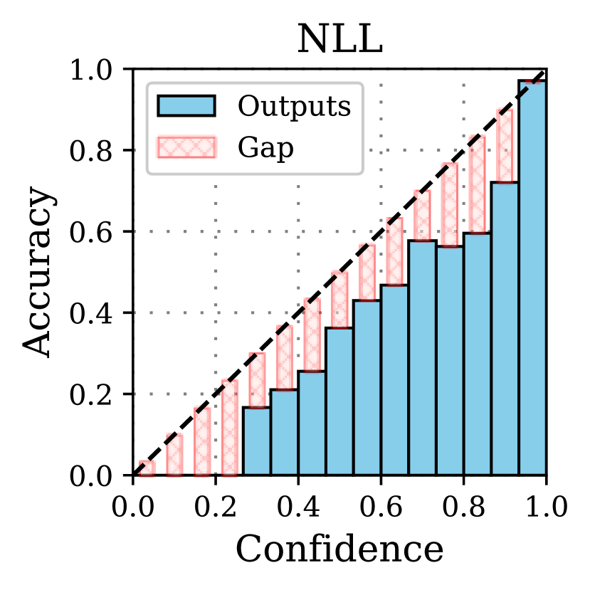
(a)

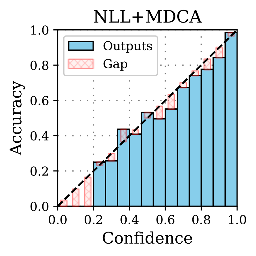
(b)

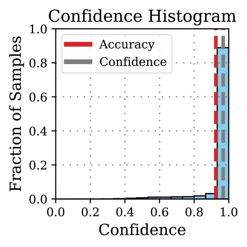
(c)

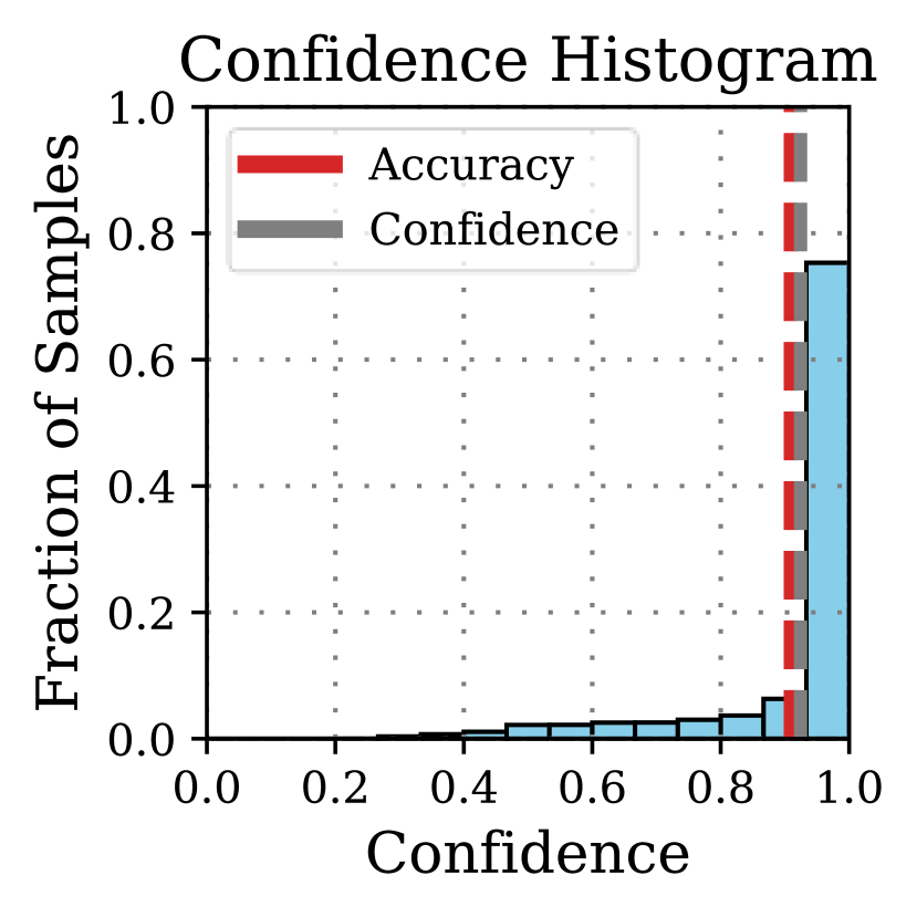
(d)

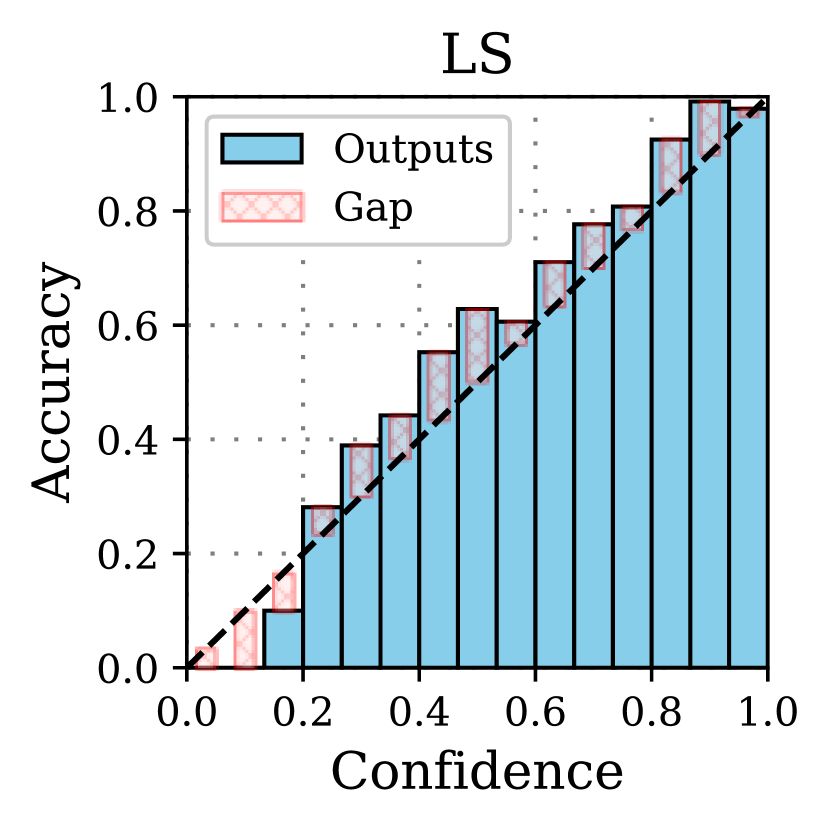
(e)

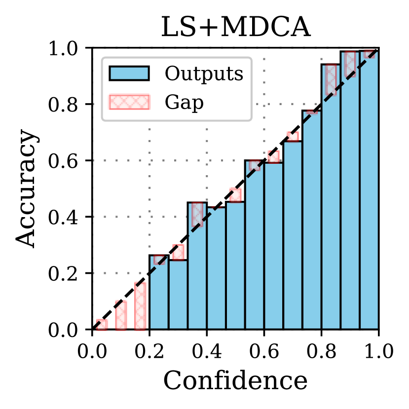
(f)

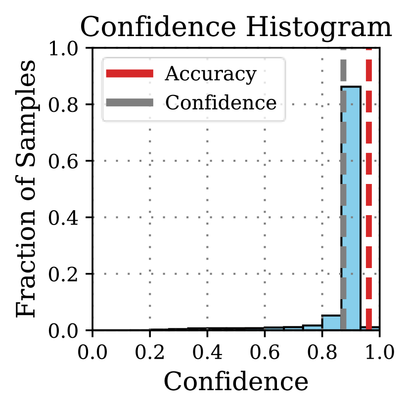
(g)

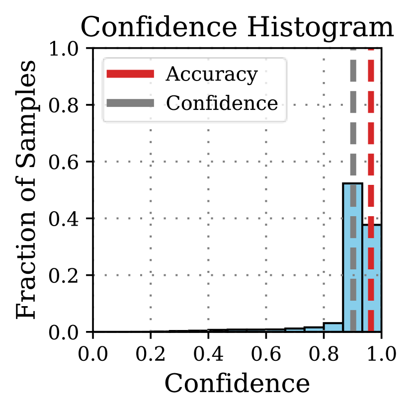
(h)

Figure 2: First row shows Reliability diagrams (a,b) and confidence histograms (c,d) of nll trained model compared against mdca regularized version (nll+mdca). We use ResNet-32 trained on CIFAR10 dataset for comparison. Second row shows corresponding plots for ResNet-20 network trained with Label Smoothing(ls) vs. mdca regularized ls on SVHN dataset. Please refer to the text for the interpretation of the plots. We show a similar comparison with fl, and fl+dca in the supplementary.

Calibration Comparison with sota: Tab. 2 compares calibration performance of our method with all recent sota methods. We note that calibration using our method improves both sce as well as ece score on all the datasets, and different architectures.

Class-Conditioned Calibration Error: Current state-of-the-art focuses on calibrating the predicted label only, which leaves some of the minority class un-calibrated. One of the benefits of our calibration approach is better calibration for all and not only the predicted class. To demonstrate the effectiveness of our method, we report class-$j$-ece % values of all the competing methods against our method, using ResNet-20 model trained on the svhn dataset. Tab. 3 shows the result. Our method gives best scores for all but 3 out of 10 classes, where it is second-best. Class-wise reliability diagrams (c.f. Fig. 1) reinforce a similar conclusion. We show results on cifar 10 dataset in the supplementary.

Test Error: Tab. 2 also shows the Test Error (te) obtained by a model trained using our method and other sota approaches. We note that using our proposed loss, a model is able to achieve best calibration performance without sacrificing on the prediction accuracy (Test Error).

Mitigating Under/Over-Confidence: Tab. 1 and Tab. 2 already show that our method improves over sota in terms of sce, and ece scores. However the tables do not highlight whether they correct for over-confidence or under-confidence. We show the reliability diagram (Fig. 2) for a ResNet-32 model trained on cifar 10. The uncalibrated model is overconfident (Fig. 2(a)) which gets rectified after calibrating with our method (Fig. 2(b)). We also show confidence plots in the picture, and the colored dashed lines to indicate average confidence of the predicted label, and the accuracy. It can be seen that accuracy is lower than average confidence in the uncalibrated confidence plot (Fig. 2(c)), which indicates the overconfident model. After calibrating with our method, the two dashed lines almost overlap indicating the perfect calibration achieved (Fig. 2(d)). Similarly, second row of Fig. 2 show that the model trained with ls solely is under-confident; and a model trained with ls along with mdca is confident and calibrated.

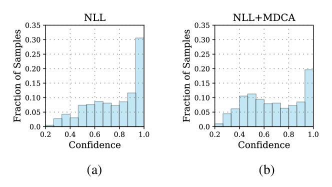
Figure 3: Confidence value histogram for misclassified predictions. mdca regularized nll makes less confident incorrect predictions as compared to the uncalibrated method trained using nll.

Confidence Values for Incorrect Predictions: The focus of the discussion so far has been on the fact that confidence value for a class should be consistent with the likelihood of the class for the sample. Here, we analyze our method for the confidence values it gives when the prediction is incorrect. Fig. 3 shows the confidence value histogram for all the incorrect predictions made by the ResNet-32 model trained on cifar 10 dataset using nll vs. mdca regularized nll. It is clear that our calibration reduces the confidence for the mis-prediction. The same is also evident from the Fig. 1 shown earlier.

Method	Art	Cartoon	Sketch	Average
NLL	6.33	17.95	15.01	13.10
LS [40]	7.80	11.95	10.88	10.21
FL [34]	8.61	16.62	10.94	12.06
Brier Score [2]	6.55	13.19	15.63	11.79
MMCE [27]	6.35	15.70	17.16	13.07
DCA [32]	7.49	18.01	14.99	13.49
FLSD [39]	8.35	13.39	13.86	11.87
Ours (FL+MDCA)	6.21	11.91	11.08	9.73

Table 4: Calibration performance (sce ($10^{-3}$)) under domain shift on pacs dataset [31]. For each column we train on the other two subsets, and then test on the subset listed as the column heading.

Method	CIFAR10			SVHN
	IF-10	IF-50	IF-100	IF-2.7
NLL	18.44	32.21	31.04	3.43
FL [34]	14.65	29.67	28.89	2.54
LS [40]	14.88	26.30	20.79	18.80
BS [2]	15.74	33.57	29.01	2.12
MMCE [27]	15.10	29.05	21.56	9.18
FLSD [39]	16.05	31.35	30.28	18.98
DCA [32]	18.57	32.81	35.53	4.29
Ours (FL+MDCA)	11.83	22.97	26.89	1.90

Table 5: Our calibration technique works best even when there is a significant class imbalance in the dataset. For this experiment we created imbalance of various degrees in cifar 10 as suggested in [6]. Original svhn has a Imbalance Factor(IF) of $2.7$. Hence we show calibration performance (sce ($10^{-3}$)) on original svhn.

Calibration Performance under Dataset Drift: Tomani et al.[52] show that dnns are over-confident and highly uncalibrated under dataset/domain shift. Our experiments shows that a model trained with mdca fairs well in terms of calibration performance even under non-semantic/natural domain shift. We use two datasets (a) pacs [31] and (b) Rotated mnist inspired from [44]. The datasets are benchmarks for synthetic non-semantic shift and natural rotations respectively. Dataset specifics and training procedure are provided in the supplementary. Tab. 4 shows that our method achieves the best average sce value across all the domains in pacs. A similar trend is observed on Rotated mnist dataset as well (see supplementary), where our method achieves the least average sce value across all rotation angles.

Calibration Performance on Imbalanced Datasets: The real-world datasets are often skewed and exhibit long-tail distributions, where a few classes dominate over the rare classes. In order to study the effect of class imbalance on the calibration quality, we conduct the following experiment, where we introduce a deliberate imbalance on cifar 10 dataset to force a long-tail distribution as detailed in [6]. Tab. 5 shows that a model trained with our method has best calibration performance in terms of sce score across all imbalance factors. We observe that svhn dataset already has a imbalance factor of $2.7$, and hence create no artificial imbalance in the dataset for this experiment. The efficacy of our approach on the imbalanced data is due to the regularization provided by mdca which penalizes the difference between average confidence and average count even for the non-predicted class, hence benefiting minority classes.

Method	Post Hoc		SCE($10^{-3}$) $\downarrow$
		CIFAR10	CIFAR100	SVHN
NLL	None	7.12	2.50	3.84
	TS	3.25	1.49	4.16
	DC	4.98	1.91	2.69
LS [40]	None	12.55	1.73	21.08
	TS	4.49	1.67	3.12
	DC	5.34	1.98	2.81
FL [34]	None	4.19	1.89	7.85
	TS	4.19	1.62	2.72
	DC	5.48	2.02	3.36
BS [2]	None	5.44	1.86	2.18
	TS	3.94	1.68	3.88
	DC	4.83	1.80	2.11
MMCE [27]	None	9.12	2.35	9.69
	TS	4.05	1.61	3.74
	DC	6.26	1.95	5.11
DCA [32]	None	7.60	2.87	2.16
	TS	3.00	1.56	4.29
	DC	4.20	2.06	2.95
FLSD [39]	None	7.71	1.71	26.15
	TS	3.27	1.71	4.41
	DC	5.62	2.01	4.31
Ours (FL+MDCA)	None	2.93	1.60	1.51
	TS	2.93	1.60	5.00
	DC	3.81	1.87	2.72

Table 6: Results after combining various trainable calibration methods including ours with two post-hoc calibration methods (ts: Temperate scaling [48], and dc: Dirichlet Calibration [24]) on sce ($10^{-3}$). We use ResNet56 model on cifar 10, cifar 100, and svhn datasets for this experiment. Though other methods benefit by post-hoc calibration, our method outperforms them without using any post-hoc calibration.

Our Approach + Post-hoc Calibration: We study the performance of combined effect of post-hoc calibration methods, namely Temperature Scaling (ts) [48], and Dirichlet Calibration (dc) [24], applied over various train-time calibration methods including ours (fl+mdca). Tab. 6 shows the results. We observe that while ts, and dc improve the performance of other competitive methods, our method outperforms them even without using any of these methods. On the other hand, the performance of our method seems to either remain same or slightly decrease after application of post-hoc methods. We speculate that this is because our method already calibrates the model to near perfection. For example, on performing ts, we observe the optimal temperature values are $T\approx 1$ implying that it leaves little scope for the TS to improve on top of it. Thus, any further attempt to over-spread the confidence prediction using ts or dc negatively affects the confidence quality.

Method	Pixel Acc. (%)	mIoU (%)	SCE ($10^{-3})$	ECE (%)
nll	94.81	79.49	6.4	7.77
nll+ts	94.81	79.49	6.26	6.1
fl	92.85	77.22	11.8	7.69
Ours (fl+mdca)	94.47	78.66	5.8	4.66

Table 7: Segmentation results on Xception65 [5] backbone DeeplabV3+ model [3] on pascal-voc 2012 validation dataset.

Calibration Results for Semantic Segmentation: One of the major advantages of our technique is that it allows to use billions of weights of a dnn model to be used for the calibration. This is in contrast to other calibration approaches which are severely constrained in terms of parameters available for tuning. For example in ts one has a single temperature parameter to tune. This makes it hard for ts to provide image and pixel specific confidence transformation for calibration. To highlight pixel specific calibration aspect of our technique we have done experiments on semantic segmentation task, which can be seen as pixel level classification. For the experiment, we train a DeepLabV3+ [3] model with a pre-trained Xception65 [5] backbone on the pascal-voc 2012 [11] dataset. We compare the performance of our method against nll, fl and ts (post-hoc calibration). Please refer to the supplementary for more details on the training. Tab. 7 shows the results. We see a significant drop in both sce/ece in case of our method (fl+mdca) as compared to fl ($2\times$ drop in sce and a 40% decrease in ece). Our method also outperforms ts (after training with nll) by $23.6\%$.

6 Ablation Study

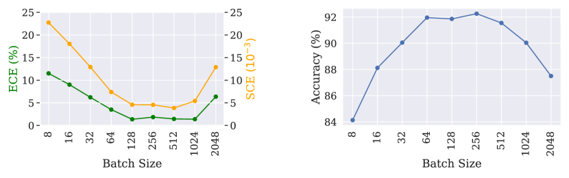
Figure 4: Effect of different batch sizes on Calibration performance metrics (ece/sce/Accuracy) while training with mdca on a ResNet-32 model on cifar 10 dataset. The calibration performance drops with larger batch size because SGD optimization is more effective in a small-batch regime[22]. A larger batch results in a degradation in the quality of the model, as measured by its ability to generalize. The performance degradation is also consistent with the model trained using solely on fl on a large batch size.

Effect of Batch Size: Fig. 4 shows the effect of different batch sizes on the calibration performance. We vary the batch sizes exponentially and observe that a model trained with mdca achieves best calibration performance around batch size of 64 or 128. As we decrease (or increase) the batch size, we see a degradation in calibration, though the drop is not significant.

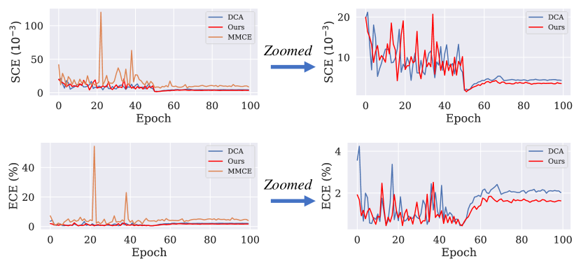
Figure 5: Comparison of ece/sce at various epochs for mdca, mmce, and dca. Though, mmce, and dca directly optimize for ece, their loss function is not differentiable and hence the techniques are not able to reduce ece as much as mdca. Differentiability of loss function allows mdca to reduce ece better even when it does not directly optimize it. We use a learning rate decay of $1/10$ at epochs $50$ and $70$. Please refer to the supplementary for the details of the experiment.

Comparison of ece/sce Convergence with sota: In previous sections, we compared the ece scores of mdca with other contemporary trainable calibration methods like mmce [27] and dca [32]. Many of these methods explicitly aim to reduce ece scores. While mdca does not directly optimize ece, yet we see in our experiments that mdca manages to get better ece scores at convergence. We speculate that this is due to the differentiablity of mdca loss which helps optimize the loss better using backpropagation. To verify the hypothesis, we plot the ece convergence for various methods in Fig. 5.

7 Conclusion & Future work

We have presented a train-time technique for calibrating the predicted confidence values of a dnn based classifier. Our approach combines standard classification loss functions with our novel auxiliary loss named, Multi-class Difference of Confidence and Accuracy (mdca). Our proposed loss function when combined with focal loss yields the least calibration error among both trainable and post-hoc calibration methods. We show promising results in case of long tail datasets, natural/synthetic dataset drift, semantic segmentation and a natural language classification benchmark too. In future we would like to investigate the role of class hierarchies to develop cost-sensitive calibration techniques.

Supplementary Material: A Stitch in Time Saves Nine: A Train-Time Regularizing Loss for Improved Neural Network Calibration

Table of Contents

Due to the restrictions on the length, we could not include descriptions of the state-of-the-art techniques, datasets, hyper-parameters and additional results in the main manuscript. However, to keep the overall manuscript self-contained, we include the following in the supplementary material:

• Section 1: Description of competing methods.

• Section 2: Detailed description of benchmark datasets used in our experiments.

• Section 3: Training procedure and implementation of proposed, and competing methods.

• Section 4: Additional results.

• Source code link: MDCA Official PyTorch Github

Appendix A Competing Methods and hyperparameters used

In this section, we provide a brief description of each of the compared method with hyperparameter settings used in training.

• For Brier Score [2] we train on the loss defined as the squared loss of the predicted probability vector and the one-hot target vector.

• Label Smoothing [40], takes the form $\texttt{LS}=-\sum_{i=1}^{N}\sum_{j=1}^{K}q_{i,j}\log(\hat{p}_{i,j})$ where $\hat{p}_{i,j}$ is the predicted confidence score for sample $i$, for class $j$. Similarly, we define soft target vector, ${q_{i}}$, for each sample $i$, such that $q_{i,j}=\alpha/(K-1)$ if $j\neq y_{i}$, else $q_{i,j}=(1-\alpha)$. Here $\alpha$ is a hyper-parameter. We trained using $\alpha=0.1$, and refer to label smoothing as LS in the results.

• Focal loss [34] is defined as $\texttt{FL}=-\sum_{i=1}^{N}(1-\hat{p}_{i,y_{i}})^{\gamma}\log(\hat{p}_{i,y_{i}})$, where $\gamma$ is a hyper-parameter. We trained using $\gamma\in\{1,2,3\}$, and report it as FL in the results.

• For DCA [32], we train on the following loss: $\texttt{NLL}+\beta\cdot\texttt{DCA}$, where DCA is as defined in [32], and $\beta$ is a hyper-parameter. We train varying $\beta\in\{1,5,10,15,20,25\}$ as performed in [32]. DCA results are reported under the name DCA.

• We use MMCE [27], as a regularizer along with NLL. We use the weighted MMCE loss in our experiments with $\lambda\in\{2,4\}$.

• For FLSD [39], we train with $\gamma=3$.

For each of the above methods, we report the result of the best performing trained model according to the accuracy obtained on the validation set.

Appendix B Dataset description

We have used the following datasets in our experiments:

1. CIFAR10 [23]: This dataset has $60,000$ color images of size $32\times 32$ each, equally divided into $10$ classes. The pre-divided train set comes with $50,000$ images and the test set has around $10,000$ images. Using the policy defined above, we have a train/val/test split having $45000/5000/10000$ images respectively.

2. CIFAR100 [23]: This dataset comprises of $60,000$ colour images of size $32x32$ each, but this time, equally divided into $100$ classes. The pre-divided train set again comes with $50,000$ images and the test set has around $10,000$ images. We have a train/val/test split having $45000/5000/10000$ images respectively.

3. SVHN [42] : The Street View House Number (SVHN) is a digit classification benchmark dataset that contains $600000$ $32\times 32$ RGB images of printed digits (from $0$ to $9$) cropped from pictures of house number plates. The cropped images are centered in the digit of interest, but nearby digits and other distractors are kept in the image. SVHN has comes with a training set ($73257$) and a testing set ($26032$). We randomly sample $10\%$ of the training set to use as a validation set.

4. Tiny-ImageNet [7] : It is a subset of the ImageNet dataset containing $64\times 64$ RGB images. It has $200$ classes with each class having $500$ images. The validation set contains $50$ images per class. We use the provided validation set as the test set for our experiments.

5. 20 Newsgroups [29]: It is a popular text classification dataset containing $20,000$ news articles, categorised evenly into $20$ different newsgroups based on their content.

6. Mendeley V2  [21]: Inspired from [32], we use this medical dataset. The dataset contains OCT (optical coherence tomography) images of retina and pediatric chest X-ray images. However, we only use the chest X-ray images in our experiments. The chest X-ray images come with a pre-defined train/test split having $4273$ pneumonia images and $1583$ normal images of the chest.

7. PACS dataset [31]: We use the dataset to study calibration under domain shift. The dataset comprises of a total $9991$ images spread across $4$ different domains with $7$ classes each. The domains are namely Photo, Art, Sketch and Cartoon. We fine-tune the ResNet-18 model, pretrained ImageNet dataset, on the Photo domain using various competing techniques and test on the other three domains to measure how calibration holds in a domain shift. Following [31], we also divide the training set of photo domain into $9:1$ train/val set.

8. Rotated MNIST Dataset: This dataset is also used for domain shift experiments. Inspired from [52], we create 5 different test sets namely $\{M_{15},M_{30},M_{45},M_{60},M_{75}\}$. Domain drift is introduced in each $M_{x}$ by rotating the images in the MNIST test set by $x$ degrees counter-clockwise.

9. Segmentation Datasets- PASCAL VOC 2012 [11]: This a segmentation dataset and consists of images with pixel-level annotations. There are 21 classes overall (One background class and 20 foreground object classes). The dataset is divided into Train (1464 images), Val (1449 images) and Test (1456 images) set. We, however, only make use of the Train and the Val set. Models are trained on the Train set and the evaluation is reported on the Val set.

Appendix C Training Procedure and Implementation

Backbone Architecture: We use ResNet [15] backbone for most of our experiments. For training on CIFAR10, and CIFAR100 datasets we used ResNet-32 and ResNet-56. For SVHN we used ResNet-20 and ResNet-56. Following [32], for Mendeley V2 dataset, we use a ResNet-50 architecture pre-trained on ImageNet dataset [7]. We use the backbone as a fixed feature extractor and add a $1\times 1$ convolutional layer and two fully connected layers on top of the feature extractor. Segmentation experiments make use of DeepLabV3+ [3] based on the Xception65 [5] backbone

Train Parameters: For all our experiments we used a single Nvidia 1080 Ti GPU. We trained CIFAR10 for a total of $160$ epochs using a learning rate of $0.1$, and it is reduced by a factor of $10$ at the $80^{th}$ and $160^{th}$ epoch. Train batch size was kept at $128$ and DNN was optimized using Stochastic Gradient Descent (SGD) with momentum at $0.9$ and weight decay being $0.0005$. Furthermore, we augment the images using random center crop and horizontal flips. We use same parameters for CIFAR100, except the number of epochs, where we train it for $200$ epochs. Again learning rate is reduced by a factor of $10$, but this time it is reduced at epochs 100 and 150. For Tiny-ImageNet, we followed the same training procedure as done by [39]. For SVHN, we keep the same training procedure as above except the number of epochs; we train for $100$ epochs, with it getting reduced at epochs $50$ and $70$ with a factor of $10$ yet again. We do not augment the images when training on SVHN. We use PyTorch framework for all our implementations. Our repository is inspired from https://github.com/bearpaw/pytorch-classification. We also take help from the official implementation of [39] to implement some of the baseline methods. For the segmentation experiments we make use of the following repository: https://github.com/LikeLy-Journey/SegmenTron. We train the segmentation models for 120 epochs using SGD optimizer with a warm-up LR scheduler. To train with focal loss, we used $\gamma=3$. The rest of the parameters for the optimizer and the scheduler were kept the same as provided by the SegmenTron repository.

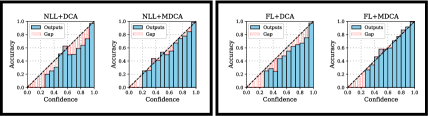
Figure 6: Comparison of Reliability diagrams of: (left) NLL+DCA vs NLL+MDCA and (right) FL+DCA vs. FL+MDCA. We use ResNet-32 trained on CIFAR10 dataset for comparison.

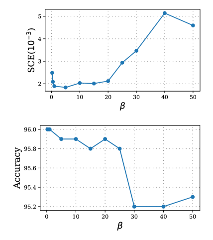
Figure 7: Effect of $\beta$ on Accuracy and SCE ($10^{-3}$) on FLL+MDCA on the ResNet-20 model trained on SVHN dataset.

Optimizing Hyper-parameter $\beta$ for MDCA: We vary the hyper-parameter $\beta\in[0.25,0.5,1,5,10,\dots 50]$ in our experiments. Figure 7 shows how calibration error and accuracy is affected when we increase $\beta$ in different model-dataset pairs. We see a general trend that calibration is best achieved when $\beta$ is close to $1$, and as we increase it, the calibration as well as the accuracy starts to drop (accuracy decreases and the SCE score increases).

Post-Hoc Calibration Experiments: For comparison with post-hoc techniques, we set aside $10\%$ of the training data as a validation set (hold-out set) to conduct post-hoc calibration. For Temperature Scaling (TS), we perform a grid search between the range of $0$ to $10$ with a step-size of $0.1$ to find the optimal temperature value that gives the least NLL on the hold-out set. For Dirichlet Calibration (DC), we attach a single layer neural network at the end of the DNN and use ODIR [24] regularization on the weights of the same. We train on the hold-out set keeping the rest of the DNN weights frozen except the newly added layer. We again use grid search to find the optimal hyper-parameters $\lambda$ and $\mu$ that give the least NLL on the hold-out set. We vary $\lambda\in\{0,0.01,0.1,1,10,0.005,0.05,0.5,5,0.0025,0.025,0.25,2.5\}$ and $\mu\in\{0,0.01,0.1,1,10\}$.

$\mathcal{L}_{C}$	$\mathcal{L}_{Auxiliary}$	Accuracy	SCE ($10^{-3}$)	ECE ($\%$)
ResNet-32 on CIFAR10 dataset:
Cross Entropy	None	92.54	8.68	4.25
	DCA [32]	92.94	8.41	4.00
	MMCE [27]	91.59	8.17	3.31
	MDCA (ours)	91.85	4.63	1.69
Label Smoothing [40]	None	92.48	14.09	6.28
	DCA [32]	88.69	8.14	3.44
	MMCE [27]	91.92	22.49	10.07
	MDCA (ours)	93.01	12.38	5.66
Focal Loss [34]	None	92.52	4.09	1.01
	DCA [32]	92.65	7.50	3.49
	MMCE [27]	90.76	26.41	13.38
	MDCA (ours)	92.82	3.22	0.93
ResNet-20 on SVHN dataset:
Cross Entropy	None	96.14	3.43	1.64
	DCA [32]	96.17	4.29	2.02
	MMCE [27]	95.88	9.18	4.34
	MDCA (ours)	96.33	1.46	0.43
Label Smoothing [40]	None	96.24	18.80	8.88
	DCA [32]	96.55	9.80	4.46
	MMCE [27]	96.11	31.75	15.50
	MDCA (ours)	96.14	13.91	6.46
Focal Loss [34]	None	96.17	2.54	0.89
	DCA [32]	96.35	2.12	0.44
	MMCE [27]	95.83	25.01	12.79
	MDCA (ours)	96.08	1.90	0.47

Table 8: Ablation to study the impact of various auxiliary losses on two models : ResNet-32 on CIFAR10 and Resnet-20 trained model on SVHN Dataset. Our approach exhibits least calibration error without sacrificing on the accuracy.

Methods	Art	Cartoon	Sketch	Average
SCE($10^{-3})$
NLL	6.33	17.95	15.01	13.10
LS [40]	7.80	11.95	10.88	10.21
FL [34]	8.61	16.62	10.94	12.06
Brier Score [2]	6.55	13.19	15.63	11.79
MMCE [27]	6.35	15.70	17.16	13.07
DCA [32]	7.49	18.01	14.99	13.49
FLSD [39]	8.35	13.39	13.86	11.87
Ours (FL+MDCA)	6.21	11.91	11.08	9.73
ECE (%)
Brier Score [2]	3.35	33.68	42.61	26.55
NLL	9.42	52.99	35.56	32.66
LS [40]	8.70	25.21	13.29	15.73
Focal Loss [34]	7.34	48.96	25.33	27.21
MMCE [27]	17.06	43.25	40.79	33.70
DCA [32]	13.38	55.20	37.76	35.45
FLSD [39]	8.41	34.43	30.01	24.28
Ours (FL+MDCA)	6.29	29.81	23.05	19.71
Top-1 (%) Accuracy
Brier Score[2]	59.28	24.83	28.43	37.51
NLL	59.08	21.20	28.00	36.09
LS[40]	56.35	22.01	29.88	36.08
FL[34]	52.83	17.32	26.70	32.28
MMCE[27]	60.60	29.95	20.36	36.97
DCA[32]	57.91	20.86	28.30	35.69
FLSD[39]	54.54	20.82	29.35	34.90
Ours (FL+MDCA)	63.23	27.86	23.01	38.03

Table 9: Table comparing SCE, ECE and Top-1% Accuracy values of our method against others on PACS [31] dataset when the model is trained on Photo domain and tested on domains: Art, Cartoon, and Sketch

Method	Clean	$M_{15}$	$M_{30}$	$M_{45}$	$M_{60}$	$M_{75}$	Average
SCE ($\%$)
NLL	0.07	0.19	0.70	2.96	7.50	10.60	3.67
LS [40]	2.00	2.00	1.93	2.91	6.67	8.93	4.07
FL [34]	0.29	0.81	1.34	2.62	7.04	10.10	3.70
Brier Score [2]	0.23	0.51	1.09	2.83	6.58	9.10	3.39
MMCE [27]	2.51	4.05	5.01	4.55	5.28	5.29	4.45
DCA [32]	0.07	0.20	0.91	3.71	8.42	11.65	4.16
FLSD [39]	1.30	2.09	3.10	3.05	4.88	7.56	3.67
Ours (FL+MDCA)	0.20	0.48	0.94	2.51	6.65	9.61	3.40
ECE ($\%$)
NLL	0.11	0.38	1.13	10.54	31.95	45.06	14.86
LS [40]	9.89	9.32	7.13	6.86	27.36	37.28	16.31
FL [34]	1.34	3.11	3.92	5.21	28.11	41.17	13.81
Brier Score [2]	0.90	2.07	2.57	5.95	25.24	38.16	12.48
MMCE [27]	4.72	15.42	23.01	18.88	10.74	6.80	13.26
DCA [32]	0.21	0.29	1.88	13.83	36.31	50.25	17.13
FLSD [39]	6.50	10.43	14.33	7.92	14.80	29.34	13.89
Ours (FL+MDCA)	0.79	2.03	2.94	6.18	25.77	39.29	12.83
Top-1 (%) Accuracy
NLL	99.61	98.79	93.38	73.82	43.24	24.07	72.15
LS [40]	99.62	98.39	92.04	69.33	39.94	22.99	70.39
FL [34]	99.63	98.20	91.87	69.95	38.67	20.83	69.86
Brier Score [2]	99.63	98.72	92.54	71.29	41.90	22.73	71.14
MMCE [27]	98.43	94.99	83.93	53.88	28.76	16.84	62.81
DCA [32]	99.60	98.36	91.51	68.34	38.32	20.93	69.51
FLSD [39]	99.67	98.79	92.77	71.17	40.17	20.84	70.57
Ours (FL+MDCA)	99.59	98.61	93.13	70.92	41.93	23.37	71.26

Table 10: Table comparing SCE, ECE and Top-1% Accuracy values of our loss with other methods on the Rotated-MNIST dataset trained using a ResNet-20 model.

Domain Shift Experiments: For PACS dataset, we use the official PyTorch ResNet-18 model pre-trained on ImageNet dataset. We re-initialized its last fully connected layer to accommodate 7 classes, and finally fine-tuned on the Photo domain. We use the SGD optimizer with same momentum and weight decay values as done for CIFAR10/100 and described earlier. Training batch size was fixed at $256$, and the model was trained for 30 epochs with initial learning rate, set at 0.01, getting reduced at epoch 20 with a factor of 10. Training parameters are chosen such that they give the best performing model i.e. having the maximum accuracy on the Photo domain val set.

For Rotated MNIST, we used PyTorch framework to generate rotated images. We use the ResNet-20 model to train on the standard MNIST train set for 30 epochs with a learning rate of 0.1 for first 20 epochs, and then with 0.01 for the last 10 epochs. Rest of the details like batch size and optimizer remain same as the CIFAR10/100 experiments. We did not augment any images, and selected the training parameters such that the model gives best accuracy on the validation set.

For 20 Newsgroups, we train the Global Pooling Convolutional Network [33] using the ADAM optimizer, with learning rate $0.001$, and the default values of betas at $0.9$ and $0.999$ respectively. We used GloVe word embeddings [46] to train the network. We trained the model for $50$ epochs.

Appendix D Additional Results

We report the following additional results:

Domain	NLL	NLL+MDCA	LS	LS+MDCA	FL	FL+MDCA
SCE ($\%$)
Clean	0.07	0.07	2.00	1.99	0.29	0.20
$M_{15}$	0.19	0.19	2.00	1.99	0.81	0.48
$M_{30}$	0.70	0.66	1.93	1.88	1.34	0.94
$M_{45}$	2.96	3.17	2.91	2.85	2.62	2.51
$M_{60}$	7.50	7.99	6.67	6.08	7.04	6.65
$M_{75}$	10.60	11.17	8.93	8.82	10.10	9.61
Average	3.67	3.88	4.07	3.94	3.70	3.40
ECE (%)
Clean	0.11	0.22	9.89	9.83	1.34	0.79
$M_{15}$	0.38	0.21	9.32	9.41	3.11	2.03
$M_{30}$	1.13	1.31	7.13	7.38	3.92	2.94
$M_{45}$	10.54	12.50	6.86	8.41	5.21	6.18
$M_{60}$	31.95	35.02	27.36	25.32	28.11	25.77
$M_{75}$	45.06	49.41	37.28	38.41	41.17	39.29
Average	14.86	16.45	16.31	16.46	13.81	12.83
Top-1 (%) Accuracy
Clean	99.61	99.64	99.62	99.63	99.63	99.59
$M_{15}$	98.79	98.63	98.39	98.45	98.20	98.61
$M_{30}$	93.38	93.23	92.04	92.54	91.87	93.13
$M_{45}$	73.82	71.53	69.33	69.74	69.95	70.92
$M_{60}$	43.24	41.27	39.94	41.88	38.67	41.93
$M_{75}$	24.07	22.05	22.99	22.97	20.83	23.37
Average	72.15	71.06	70.39	70.87	69.86	71.26

Table 11: Table comparing SCE, ECE and Top-1% Accuracy values of our method against others for ResNet-20 model on Rotated-MNIST dataset. Clean denotes the original dataset, and subscript under the ‘M’ indicates angle of rotation for each digit.

Domain	NLL	NLL+MDCA	LS	LS+MDCA	FL	FL+MDCA
SCE ($10^{-3}$)
Art	6.33	5.10	7.80	5.70	8.61	6.21
Cartoon	17.95	16.53	11.95	12.07	16.22	11.91
Sketch	15.01	13.49	10.88	11.70	10.94	11.08
Average	13.10	11.71	10.21	9.82	12.06	9.73
ECE (%)
Art	9.42	4.99	8.70	11.80	7.34	6.29
Cartoon	52.99	47.96	25.21	22.73	48.96	29.81
Sketch	35.56	31.68	13.29	10.34	25.33	23.05
Average	32.66	28.21	15.73	14.96	27.21	19.71
Top-1 (%) Accuracy
Art	59.08	61.67	56.35	59.57	52.83	63.23
Cartoon	21.20	21.72	22.01	24.62	17.32	27.86
Sketch	28.00	26.90	29.88	26.55	26.70	23.01
Average	36.09	36.76	36.08	36.91	32.28	38.03

Table 12: Ablation comparing SCE, ECE and Top-1 Accuracy values of models using MDCA as an auxiliary loss along with other classification losses. The numbers correspond to training a ResNet-18 model on Photo subset from PACS dataset, and testing on other subsets of the PACS.

1. Class-j-ECE score: In Table 3 of main manuscript we reported the Class-j-ECE score for SVHN. In Table 13 here, we we provide additional results for CIFAR10.

2. Comparison with other auxiliary losses: In Table 6 in the main manuscript showed how the proposed MDCA can be used along with NLL, LS [50], and FL [34] to improve the calibration performance without sacrificing the accuracy. In Tab. 8 here, we show a similar comparison for other competitive approaches, namely DCA [32], and MMCE [27]. Using MDCA, gives better calibration than other competitive approaches.

3. Calibration performance under dataset drift: A model trained using our proposed loss gives better calibration under dataset drift as well. Table 4 in the main manuscript showed SCE score comparison on PACS. We give more detailed comparison here in Tab. 9 which shows top 1% accuracy, ECE as well. We repeat SCE numbers from main manuscript for completion. Tab. 10 shows the corresponding numbers for Rotated MNIST.

   Just like we showed that using MDCA in conjunction with NLL, LS [50], and FL [34] gives best calibration performance, we show that this remains true even for the dataset drift case. Tab. 11 and Tab. 12 show the comparison on Rotated MNIST and PACS datasets respectively.

4. Reliability Diagrams: Fig. 2 in the main manuscript showed reliability and confidence plots for MDCA used with NLL and LS respectively. We show similar plots for MDCA+FL in Fig. 8.

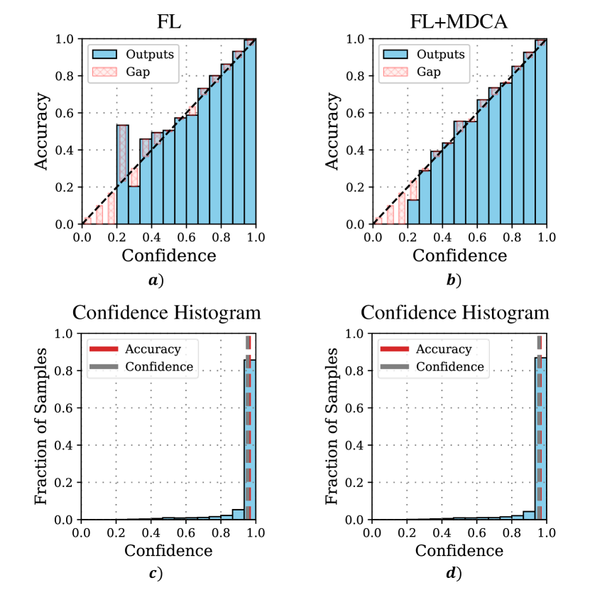
Figure 8: Reliability diagrams (a,b) and confidence histograms (c,d) of FL trained model compared against MDCA regularized version (FL+MDCA). We use ResNet-32 trained on CIFAR10 dataset for comparison.

Method	Classes
	airplane	automobile	bird	cat	deer	dog	frog	horse	ship	truck
Cross Entropy	0.98	0.43	1.12	1.97	0.65	1.47	0.65	0.44	0.58	0.57
Focal Loss [34]	0.38	0.23	0.69	1.08	0.39	0.91	0.37	0.34	0.25	0.24
LS [40]	1.64	1.89	1.26	1.01	1.64	1.25	1.66	1.62	1.76	1.77
Brier Score [2]	0.71	0.25	0.91	1.56	0.61	1.26	0.4	0.34	0.41	0.37
MMCE [27]	1.88	1.29	1.57	2.43	1.83	1.62	1.57	1.51	1.09	1.75
DCA [32]	0.80	0.43	1.18	1.71	0.93	1.44	0.52	0.55	0.51	0.6
FLSD [39]	0.99	1.12	0.81	1.11	0.81	1.44	0.81	0.85	0.70	1.14
Ours (FL+MDCA)	0.36	0.37	0.36	0.60	0.35	0.59	0.31	0.41	0.25	0.42

Table 13: Class-$j$-ECE (%) values on all ten classes for a ResNet-32 model trained on the CIFAR10 dataset comparing different learnable calibration methods including ours highlighted in Cyan.

References

- [1] Ondrej Bohdal, Yongxin Yang, and Timothy Hospedales. Meta-calibration: Meta-learning of model calibration using differentiable expected calibration error. 2021.
- [2] Glenn W Brier et al. Verification of forecasts expressed in terms of probability. Monthly weather review, 78(1):1–3, 1950.
- [3] Liang-Chieh Chen, Yukun Zhu, George Papandreou, Florian Schroff, and Hartwig Adam. Encoder-decoder with atrous separable convolution for semantic image segmentation. CoRR, abs/1802.02611, 2018.
- [4] Liang-Chieh Chen, George Papandreou, Iasonas Kokkinos, Kevin Murphy, and Alan L. Yuille. Deeplab: Semantic image segmentation with deep convolutional nets, atrous convolution, and fully connected crfs. IEEE Transactions on Pattern Analysis and Machine Intelligence, 40(4):834–848, 2018.
- [5] François Chollet. Xception: Deep learning with depthwise separable convolutions. In Proceedings of the IEEE conference on computer vision and pattern recognition, pages 1251–1258, 2017.
- [6] Yin Cui, Menglin Jia, Tsung-Yi Lin, Yang Song, and Serge Belongie. Class-balanced loss based on effective number of samples. In 2019 IEEE/CVF Conference on Computer Vision and Pattern Recognition (CVPR), pages 9260–9269, 2019.
- [7] Jia Deng, Wei Dong, Richard Socher, Li-Jia Li, Kai Li, and Li Fei-Fei. Imagenet: A large-scale hierarchical image database. In 2009 IEEE conference on computer vision and pattern recognition, pages 248–255. Ieee, 2009.
- [8] Terrance DeVries and Graham W Taylor. Learning confidence for out-of-distribution detection in neural networks. arXiv preprint arXiv:1802.04865, 2018.
- [9] Zhipeng Ding, Xu Han, Peirong Liu, and Marc Niethammer. Local temperature scaling for probability calibration. CoRR, abs/2008.05105, 2020.
- [10] Michael W. Dusenberry, Dustin Tran, Edward Choi, Jonas Kemp, Jeremy Nixon, Ghassen Jerfel, Katherine Heller, and Andrew M. Dai. Analyzing the role of model uncertainty for electronic health records. Proceedings of the ACM Conference on Health, Inference, and Learning, Apr 2020.
- [11] M. Everingham, L. Van Gool, C. K. I. Williams, J. Winn, and A. Zisserman. The PASCAL Visual Object Classes Challenge 2012 (VOC2012) Results. http://www.pascal-network.org/challenges/VOC/voc2012/workshop/index.html.
- [12] Arthur Gretton. Introduction to rkhs, and some simple kernel algorithms. Adv. Top. Mach. Learn. Lecture Conducted from University College London, 16:5–3, 2013.
- [13] Sorin Grigorescu, Bogdan Trasnea, Tiberiu Cocias, and Gigel Macesanu. A survey of deep learning techniques for autonomous driving. Journal of Field Robotics, 37(3):362–386, 2020.
- [14] Chuan Guo, Geoff Pleiss, Yu Sun, and Kilian Q Weinberger. On calibration of modern neural networks. 2019.
- [15] Kaiming He, Xiangyu Zhang, Shaoqing Ren, and Jian Sun. Deep residual learning for image recognition, 2015.
- [16] Dan Hendrycks and Kevin Gimpel. A baseline for detecting misclassified and out-of-distribution examples in neural networks. CoRR, abs/1610.02136, 2016.
- [17] Dan Hendrycks, Mantas Mazeika, and Thomas Dietterich. Deep anomaly detection with outlier exposure. ICLR, 2018.
- [18] Geoffrey Hinton, Oriol Vinyals, and Jeff Dean. Distilling the knowledge in a neural network. arXiv preprint arXiv:1503.02531, 2015.
- [19] Mobarakol Islam, Lalithkumar Seenivasan, Hongliang Ren, and Ben Glocker. Class-distribution-aware calibration for long-tailed visual recognition. ICML Uncertainity in Deep Learning Workshop, 2021.
- [20] Davood Karimi and Ali Gholipour. Improving calibration and out-of-distribution detection in medical image segmentation with convolutional neural networks. CoRR, abs/2004.06569, 2020.
- [21] Daniel Kermany, Kang Zhang, Michael Goldbaum, et al. Labeled optical coherence tomography (oct) and chest x-ray images for classification. Mendeley data, 2(2), 2018.
- [22] N. Keskar, D. Mudigere, J. Nocedal, M. Smelyanskiy, and P. Tang. On large-batch training for deep learning: Generalization gap and sharp minima. In ICLR, 2017.
- [23] Alex Krizhevsky, Geoffrey Hinton, et al. Learning multiple layers of features from tiny images. 2009.
- [24] Meelis Kull, Miquel Perello-Nieto, Markus Kängsepp, Hao Song, Peter Flach, et al. Beyond temperature scaling: Obtaining well-calibrated multiclass probabilities with dirichlet calibration. arXiv preprint arXiv:1910.12656, 2019.
- [25] Meelis Kull, Telmo Silva Filho, and Peter Flach. Beta calibration: a well-founded and easily implemented improvement on logistic calibration for binary classifiers. In Artificial Intelligence and Statistics, pages 623–631. PMLR, 2017.
- [26] Ananya Kumar, Percy Liang, and Tengyu Ma. Verified uncertainty calibration. arXiv preprint arXiv:1909.10155, 2019.
- [27] Aviral Kumar, Sunita Sarawagi, and Ujjwal Jain. Trainable calibration measures for neural networks from kernel mean embeddings. In Jennifer Dy and Andreas Krause, editors, Proceedings of the 35th International Conference on Machine Learning, volume 80 of Proceedings of Machine Learning Research, pages 2805–2814. PMLR, 10–15 Jul 2018.
- [28] Ken Lang. Newsweeder: Learning to filter netnews. In Proceedings of the Twelfth International Conference on Machine Learning, pages 331–339, 1995.
- [29] Ken Lang. Newsweeder: Learning to filter netnews. In Machine Learning Proceedings 1995, pages 331–339. Elsevier, 1995.
- [30] Yann LeCun, Corinna Cortes, and CJ Burges. Mnist handwritten digit database. ATT Labs [Online]. Available: http://yann.lecun.com/exdb/mnist, 2, 2010.
- [31] Da Li, Yongxin Yang, Yi-Zhe Song, and Timothy M Hospedales. Deeper, broader and artier domain generalization. In Proceedings of the IEEE international conference on computer vision, pages 5542–5550, 2017.
- [32] Gongbo Liang, Yu Zhang, Xiaoqin Wang, and Nathan Jacobs. Improved trainable calibration method for neural networks on medical imaging classification. CoRR, abs/2009.04057, 2020.
- [33] Min Lin, Qiang Chen, and Shuicheng Yan. Network in network. arXiv preprint arXiv:1312.4400, 2013.
- [34] Tsung-Yi Lin, Priya Goyal, Ross Girshick, Kaiming He, and Piotr Dollár. Focal loss for dense object detection. In Proceedings of the IEEE international conference on computer vision, pages 2980–2988, 2017.
- [35] Juan Maroñas, Daniel Ramos, and Roberto Paredes. On calibration of mixup training for deep neural networks. In Joint IAPR International Workshops on Statistical Techniques in Pattern Recognition (SPR) and Structural and Syntactic Pattern Recognition (SSPR), pages 67–76. Springer, 2021.
- [36] H. Matthias, A. Maksym, and B. Julian. Why relu networks yield high-confidence predictions far away from the training data and how to mitigate the problem. In Proceedings of the IEEE/CVF Conference on Computer Vision and Pattern Recognition, pages 41–50, 2019.
- [37] Lassi Meronen, Christabella Irwanto, and Arno Solin. Stationary activations for uncertainty calibration in deep learning. arXiv preprint arXiv:2010.09494, 2020.
- [38] Matthias Minderer, Josip Djolonga, Rob Romijnders, Frances Hubis, Xiaohua Zhai, Neil Houlsby, Dustin Tran, and Mario Lucic. Revisiting the calibration of modern neural networks. arXiv preprint arXiv:2106.07998, 2021.
- [39] Jishnu Mukhoti, Viveka Kulharia, Amartya Sanyal, Stuart Golodetz, Philip H. S. Torr, and Puneet K. Dokania. Calibrating deep neural networks using focal loss, 2020.
- [40] Rafael Müller, Simon Kornblith, and Geoffrey Hinton. When does label smoothing help? arXiv preprint arXiv:1906.02629, 2019.
- [41] Mahdi Pakdaman Naeini, Gregory Cooper, and Milos Hauskrecht. Obtaining well calibrated probabilities using bayesian binning. In Twenty-Ninth AAAI Conference on Artificial Intelligence, 2015.
- [42] Yuval Netzer, Tao Wang, Adam Coates, Alessandro Bissacco, Bo Wu, and Andrew Y Ng. Reading digits in natural images with unsupervised feature learning. 2011.
- [43] Jeremy Nixon, Michael W Dusenberry, Linchuan Zhang, Ghassen Jerfel, and Dustin Tran. Measuring calibration in deep learning. In CVPR Workshops, volume 2, 2019.
- [44] Yaniv Ovadia, Emily Fertig, Jie Ren, Zachary Nado, David Sculley, Sebastian Nowozin, Joshua V Dillon, Balaji Lakshminarayanan, and Jasper Snoek. Can you trust your model’s uncertainty? evaluating predictive uncertainty under dataset shift. arXiv preprint arXiv:1906.02530, 2019.
- [45] Shreyas Padhy, Zachary Nado, Jie Ren, Jeremiah Liu, Jasper Snoek, and Balaji Lakshminarayanan. Revisiting one-vs-all classifiers for predictive uncertainty and out-of-distribution detection in neural networks. arXiv preprint arXiv:2007.05134, 2020.
- [46] Jeffrey Pennington, Richard Socher, and Christopher D Manning. Glove: Global vectors for word representation. In Proceedings of the 2014 conference on empirical methods in natural language processing (EMNLP), pages 1532–1543, 2014.
- [47] Gabriel Pereyra, George Tucker, Jan Chorowski, Lukasz Kaiser, and Geoffrey Hinton. Regularizing neural networks by penalizing confident output distributions, 2017.
- [48] John Platt et al. Probabilistic outputs for support vector machines and comparisons to regularized likelihood methods. Advances in large margin classifiers, 10(3):61–74, 1999.
- [49] Monika Sharma, Oindrila Saha, Anand Sriraman, Ramya Hebbalaguppe, Lovekesh Vig, and Shirish Karande. Crowdsourcing for chromosome segmentation and deep classification. In 2017 IEEE Conference on Computer Vision and Pattern Recognition Workshops (CVPRW), pages 786–793, 2017.
- [50] Christian Szegedy, Vincent Vanhoucke, Sergey Ioffe, Jonathon Shlens, and Zbigniew Wojna. Rethinking the inception architecture for computer vision, 2015.
- [51] Sunil Thulasidasan, Gopinath Chennupati, Jeff Bilmes, Tanmoy Bhattacharya, and Sarah Michalak. On mixup training: Improved calibration and predictive uncertainty for deep neural networks. arXiv preprint arXiv:1905.11001, 2019.
- [52] Christian Tomani, Sebastian Gruber, Muhammed Ebrar Erdem, Daniel Cremers, and Florian Buettner. Post-hoc uncertainty calibration for domain drift scenarios. CoRR, abs/2012.10988, 2020.
- [53] David Widmann, Fredrik Lindsten, and Dave Zachariah. Calibration tests in multi-class classification: A unifying framework. arXiv preprint arXiv:1910.11385, 2019.
- [54] Ronald Yu and Gabriele Spina Alì. What’s inside the black box? ai challenges for lawyers and researchers. Legal Information Management, 19(1):2–13, 2019.
- [55] Hongyi Zhang, Moustapha Cissé, Yann N. Dauphin, and David Lopez-Paz. mixup: Beyond empirical risk minimization. In ICLR, 2018.