[a]Eleftheria Malami

Puzzles in the Bs0โ†’Dsยฑโ€‹Kโˆ“โ†’subscriptsuperscript๐ต0๐‘ superscriptsubscript๐ท๐‘ plus-or-minussuperscript๐พminus-or-plusB^{0}_{s}\rightarrow D_{s}^{\pm}K^{\mp} System

Robert Fleischer โ€ƒโ€ƒ
Abstract

Non-leptonic Bs0โ†’Dsยฑโ€‹Kโˆ“โ†’subscriptsuperscript๐ต0๐‘ superscriptsubscript๐ท๐‘ plus-or-minussuperscript๐พminus-or-plusB^{0}_{s}\rightarrow D_{s}^{\pm}K^{\mp} transitions are particularly interesting processes to test the Standard Model. As these decays occur via pure tree diagrams, they allow a theoretically clean determination of the angle $\gamma$ of the unitarity triangle. Considering recent LHCb results, an intriguing picture arises, showing tension with the Standard Model. Extracting the branching ratios of the underlying Bยฏs0โ†’Dsยฑโ€‹Kโˆ“โ†’subscriptsuperscriptยฏ๐ต0๐‘ superscriptsubscript๐ท๐‘ plus-or-minussuperscript๐พminus-or-plus\bar{B}^{0}_{s}\rightarrow D_{s}^{\pm}K^{\mp} modes and combining them with information from semileptonic B(s)subscript๐ต๐‘ B_{(s)} decays, we arrive at another puzzling situation, in accordance with similar decays. These patterns could be footprints of New Physics. We present a model-independent strategy to include such New-Physics effects and apply it to the data. Interestingly, new contributions of moderate size could accommodate the data. This formalism offers an exciting probe for new sources of CP violation at the future high-precision B physics era.

1 Introduction

Decays of B mesons are very important to test the flavour sector of the Standard Model (SM) and to explore CP violation. Particularly interesting channels for such studies are the Bs0โ†’Dsโˆ“โ€‹Kยฑโ†’subscriptsuperscript๐ต0๐‘ superscriptsubscript๐ท๐‘ minus-or-plussuperscript๐พplus-or-minusB^{0}_{s}\to D_{s}^{\mp}K^{\pm} decays [1, 2, 3]. In the SM, these modes originate only from tree topologies and offer a theoretically clean determination of the angle $\gamma$ of the Unitarity Triangle (UT). Due to Bs0subscriptsuperscript๐ต0๐‘ B^{0}_{s}โ€“Bยฏs0subscriptsuperscriptยฏ๐ต0๐‘ \bar{B}^{0}_{s} oscillations, interference effects arise between the decay channels Bยฏs0โ†’Ds+โ€‹Kโˆ’โ†’subscriptsuperscriptยฏ๐ต0๐‘ superscriptsubscript๐ท๐‘ superscript๐พ\bar{B}^{0}_{s}\to D_{s}^{+}K^{-} and Bs0โ†’Ds+โ€‹Kโˆ’โ†’subscriptsuperscript๐ต0๐‘ superscriptsubscript๐ท๐‘ superscript๐พB^{0}_{s}\to D_{s}^{+}K^{-}, leading to the following time-dependent rate asymmetry for the $f$ final state Ds+โ€‹Kโˆ’superscriptsubscript๐ท๐‘ superscript๐พD_{s}^{+}K^{-}:

๐’œCโ€‹Pโ€‹(t)=ฮ“โ€‹(Bs0โ€‹(t)โ†’f)โˆ’ฮ“โ€‹(Bยฏs0โ€‹(t)โ†’f)ฮ“โ€‹(Bs0โ€‹(t)โ†’f)+ฮ“โ€‹(Bยฏs0โ€‹(t)โ†’f)=Cโ€‹cosโก(ฮ”โ€‹Msโ€‹t)+Sโ€‹sinโก(ฮ”โ€‹Msโ€‹t)coshโก(ysโ€‹t/ฯ„Bs)+๐’œฮ”โ€‹ฮ“โ€‹sinhโก(ysโ€‹t/ฯ„Bs),subscript๐’œ๐ถ๐‘ƒ๐‘กฮ“โ†’subscriptsuperscript๐ต0๐‘ ๐‘ก๐‘“ฮ“โ†’subscriptsuperscriptยฏ๐ต0๐‘ ๐‘ก๐‘“ฮ“โ†’subscriptsuperscript๐ต0๐‘ ๐‘ก๐‘“ฮ“โ†’subscriptsuperscriptยฏ๐ต0๐‘ ๐‘ก๐‘“๐ถฮ”subscript๐‘€๐‘ ๐‘ก๐‘†ฮ”subscript๐‘€๐‘ ๐‘กsubscript๐‘ฆ๐‘ ๐‘กsubscript๐œsubscript๐ต๐‘ subscript๐’œฮ”ฮ“subscript๐‘ฆ๐‘ ๐‘กsubscript๐œsubscript๐ต๐‘ \mathcal{A}_{CP}(t)=\frac{\Gamma(B^{0}_{s}(t)\to f)-\Gamma(\bar{B}^{0}_{s}(t)\to f)}{\Gamma(B^{0}_{s}(t)\to f)+\Gamma(\bar{B}^{0}_{s}(t)\to f)}=\frac{{{C}}\,\cos(\Delta M_{s}\,t)+{S}\,\sin(\Delta M_{s}\,t)}{\cosh(y_{s}\,t/\tau_{B_{s}})+{\cal A}_{\Delta\Gamma}\,\sinh(y_{s}\,t/\tau_{B_{s}})}, (1)

where we introduce the observables $C$, $S$ and ${\cal A}_{\Delta\Gamma}$. A similar relation holds for the CP-conjugate case with the $\overline{C}$, $\overline{S}$ and $\overline{{\cal A}}_{\Delta\Gamma}$ observables.

An intriguing value of $\gamma=\left(128^{+17}_{-22}\right)^{\circ}$, modulo $180^{\circ}$, which was reported by LHCb [4], was our motivation to further explore this system. Despite the significant uncertainty, this value is still much larger than the finding of global SM analyses of the UT, which give a value in the regime of $70^{\circ}$ [5, 6]. A similar range is also found in a recent simultaneous LHCb analysis of various B decays [7]. However, these decays have different dynamics and are characterised by different interference effects. We are interested in shedding more light on the question: could this unexpectedly large value of $\gamma$ imply new sources of CP violation from physics beyond the SM?

2 Determining the angle $\gamma$

Let us have a closer look at $\gamma$. We introduce the parameter $\xi$ [2]:

ฮพโˆโˆ’eโˆ’iโ€‹ฯ•sโ€‹[Aโ€‹(Bยฏs0โ†’Ds+โ€‹Kโˆ’)/Aโ€‹(Bs0โ†’Ds+โ€‹Kโˆ’)]proportional-to๐œ‰superscript๐‘’๐‘–subscriptitalic-ฯ•๐‘ delimited-[]๐ดโ†’subscriptsuperscriptยฏ๐ต0๐‘ superscriptsubscript๐ท๐‘ superscript๐พ๐ดโ†’subscriptsuperscript๐ต0๐‘ superscriptsubscript๐ท๐‘ superscript๐พ\xi\propto-e^{-i\phi_{s}}[{A(\overline{B}^{0}_{s}\rightarrow D_{s}^{+}K^{-})}/{A(B^{0}_{s}\rightarrow D_{s}^{+}K^{-})}] (2)

and similarly $\bar{\xi}$ for the $\bar{f}$ final state K+โ€‹Dsโˆ’superscript๐พsuperscriptsubscript๐ท๐‘ K^{+}D_{s}^{-}. These quantities are physical observables that measure the strength of the interference effects. The phase ฯ•ssubscriptitalic-ฯ•๐‘ \phi_{s} is the CP-violating Bs0subscriptsuperscript๐ต0๐‘ B^{0}_{s}โ€“Bยฏs0subscriptsuperscriptยฏ๐ต0๐‘ \bar{B}^{0}_{s} mixing phase and can be determined through Bs0โ†’J/ฯˆโ€‹ฯ•โ†’subscriptsuperscript๐ต0๐‘ ๐ฝ๐œ“italic-ฯ•B^{0}_{s}\to J/\psi\phi and similar modes. With the help of the measured values of the observables introduced in Eq.ย 1, for which:

$$C=({1-|\xi|^{2}})/({1+|\xi|^{2}}),\quad S=({2\,\text{Im}{\,\xi}})/({1+|\xi|^{2}}),\quad\mathcal{A}_{\Delta\Gamma}=({2\,\text{Re}\,\xi})/({1+|\xi|^{2}}),$$ (3)

we can pin down $\xi$ (and similarly $\bar{\xi}$) unambiguously. Assuming the SM expressions for the decay amplitudes leads to the theoretically clean relation

ฮพร—ฮพยฏ=eโˆ’iโ€‹2โ€‹(ฯ•s+ฮณ),๐œ‰ยฏ๐œ‰superscript๐‘’๐‘–2subscriptitalic-ฯ•๐‘ ๐›พ{\xi}\times\bar{\xi}=e^{-i2(\phi_{s}+\gamma)}\ , (4)

which allows a clean extraction of ฯ•s+ฮณsubscriptitalic-ฯ•๐‘ ๐›พ\phi_{s}+\gamma. LHCb performed a sophisticated fit to their data, assuming $C+\overline{C}=0$, which holds in SM, and obtained $\gamma=\left(128^{+17}_{-22}\right)^{\circ}$. Using ฯ•s=(โˆ’5โˆ’1.5+1.6)โˆ˜subscriptitalic-ฯ•๐‘ superscriptsubscriptsuperscript51.61.5\phi_{s}=\left(-5^{+1.6}_{-1.5}\right)^{\circ}, including penguin corrections to Bs0โ†’J/ฯˆโ€‹ฯ•โ†’subscriptsuperscript๐ต0๐‘ ๐ฝ๐œ“italic-ฯ•B^{0}_{s}\to J/\psi\phi modes [8], we find the following result [9, 10]:

$$\gamma=\left(131^{+17}_{-22}\right)^{\circ}\ {\text{[modulo $180^{\circ}$]}}.$$ (5)

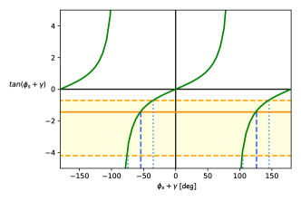
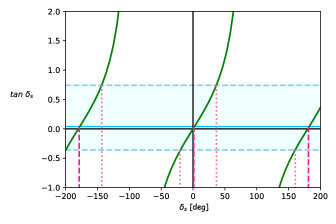
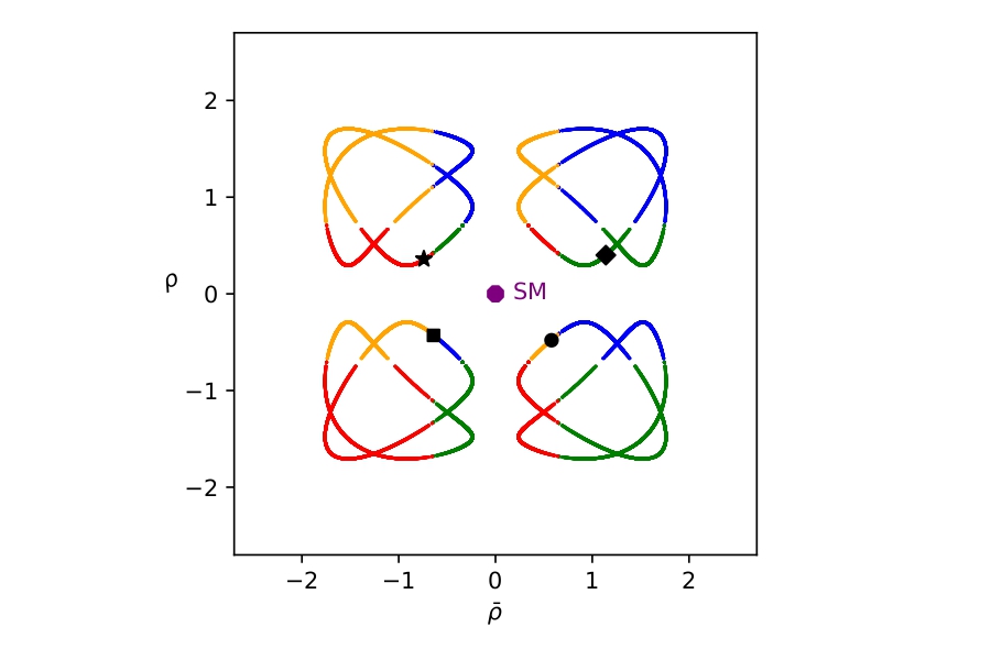
In view of the tension of this value with the SM, we need to transparently understand the situation. For this purpose, we utilise the following expressions:

tanโก(ฯ•s+ฮณ)=โˆ’โŸจSโŸฉ+/โŸจ๐’œฮ”โ€‹ฮ“โŸฉ+=โˆ’1.45โˆ’2.76+0.73,tanโกฮดs=โŸจSโŸฉโˆ’/โŸจ๐’œฮ”โ€‹ฮ“โŸฉ+=0.04โˆ’0.40+0.70formulae-sequencesubscriptitalic-ฯ•๐‘ ๐›พsubscriptdelimited-โŸจโŸฉ๐‘†subscriptdelimited-โŸจโŸฉsubscript๐’œฮ”ฮ“subscriptsuperscript1.450.732.76subscript๐›ฟ๐‘ subscriptdelimited-โŸจโŸฉ๐‘†subscriptdelimited-โŸจโŸฉsubscript๐’œฮ”ฮ“subscriptsuperscript0.040.700.40\tan(\phi_{s}+\gamma)=-\langle S\rangle_{+}/\langle\mathcal{A}_{\Delta\Gamma}\rangle_{+}=-1.45^{+0.73}_{-2.76},\quad\tan\delta_{s}=\langle S\rangle_{-}/\langle\mathcal{A}_{\Delta\Gamma}\rangle_{+}=0.04^{+0.70}_{-0.40}\ (6)

with $\langle S\rangle_{\pm}\equiv(\overline{S}\pm S)/2$ and $\langle\mathcal{A}_{\Delta\Gamma}\rangle_{+}\equiv(\overline{{\cal A}}_{\Delta\Gamma}+{\cal A}_{\Delta\Gamma})/2$, allowing us to determine ฯ•s+ฮณsubscriptitalic-ฯ•๐‘ ๐›พ\phi_{s}+\gamma and ฮดssubscript๐›ฟ๐‘ \delta_{s} as shown in Fig.1. We find excellent agreement between this transparent picture and the LHCb fit, confirming the intriguing picture.

Refer to caption
Refer to caption
Figure 1: Illustration of tanโก(ฯ•s+ฮณ)subscriptitalic-ฯ•๐‘ ๐›พ\tan(\phi_{s}+\gamma) (left) and tanโกฮดssubscript๐›ฟ๐‘ \tan\delta_{s} (right), where the horizontal lines correspond to Eq. 6.

3 Branching ratio information

The CP-violating observables can be complemented with information from branching ratios, which gives rise to a second puzzling case. We determine the individual branching ratios for the different decay channels. Assuming that $C=-\overline{C}$, in agreement with the LHCb assumption, we obtain the relation between the theoretical and experimental branching ratios [3]:

โ„ฌth=โ„ฌยฏth=[1โˆ’ys21+ysโ€‹โŸจ๐’œฮ”โ€‹ฮ“โŸฉ+]โ€‹โŸจโ„ฌexpโŸฉ,whereโŸจโ„ฌexpโŸฉโ‰ก12โ€‹(โ„ฌexp+โ„ฌยฏexp)=12โ€‹โ„ฌฮฃexp.formulae-sequencesubscriptโ„ฌthsubscriptยฏโ„ฌthdelimited-[]1superscriptsubscript๐‘ฆ๐‘ 21subscript๐‘ฆ๐‘ subscriptdelimited-โŸจโŸฉsubscript๐’œฮ”ฮ“delimited-โŸจโŸฉsubscriptโ„ฌexpwheredelimited-โŸจโŸฉsubscriptโ„ฌexp12subscriptโ„ฌexpsubscriptยฏโ„ฌexp12subscriptsuperscriptโ„ฌexpฮฃ\mathcal{B}_{\text{th}}=\bar{\mathcal{B}}_{\text{th}}=\left[\frac{1-y_{s}^{2}}{1+y_{s}\langle{\cal A}_{\Delta\Gamma}\rangle_{+}}\right]\langle\mathcal{B}_{\text{exp}}\rangle,\ \ {\text{where}}\ \ \langle\mathcal{B}_{\text{exp}}\rangle\equiv\frac{1}{2}\left(\mathcal{B}_{\text{exp}}+\bar{\mathcal{B}}_{\text{exp}}\right)=\frac{1}{2}\,\mathcal{B}^{\text{exp}}_{\Sigma}. (7)

Here we use the average $\mathcal{B}^{\text{exp}}_{\Sigma}=(2.27\pm 0.19)\times 10^{-4}$ [6] while $\langle\mathcal{A}_{\Delta\Gamma}\rangle_{\pm}=0.35\pm 0.23$ [9, 10] and ysโ‰กฮ”โ€‹ฮ“s/(2โ€‹ฮ“s)=0.062ยฑ0.004subscript๐‘ฆ๐‘ ฮ”subscriptฮ“๐‘ 2subscriptฮ“๐‘ plus-or-minus0.0620.004y_{s}\equiv\Delta\Gamma_{s}/(2\Gamma_{s})=0.062\pm 0.004 [6]. We determine $\mathcal{B}_{\text{th}}$ and finally obtain [9, 10]:

โ„ฌโ€‹(Bยฏs0โ†’Ds+โ€‹Kโˆ’)thโ„ฌsubscriptโ†’subscriptsuperscriptยฏ๐ต0๐‘ superscriptsubscript๐ท๐‘ superscript๐พth\displaystyle\mathcal{B}(\bar{B}^{0}_{s}\to D_{s}^{+}K^{-})_{\text{th}} $\displaystyle=2\left[{|\xi|^{2}}/{\left(1+|\xi|^{2}\right)}\right]\mathcal{B}_{\text{th}}=(1.94\pm 0.21)\times 10^{-4},$ (8)
โ„ฌโ€‹(Bs0โ†’Ds+โ€‹Kโˆ’)thโ„ฌsubscriptโ†’subscriptsuperscript๐ต0๐‘ superscriptsubscript๐ท๐‘ superscript๐พth\displaystyle\mathcal{B}(B^{0}_{s}\to D_{s}^{+}K^{-})_{\text{th}} $\displaystyle=2\left[{1}/{\left(1+|\xi|^{2}\right)}\right]\mathcal{B}_{\text{th}}=(0.26\pm 0.12)\times 10^{-4}.$ (9)

For the theoretical SM interpretation, these branching ratios are converted into quantities $|a_{1}|$, which are phenomenological colour factors that characterise colour-allowed tree decays. Our goal is to extract these parameters in a way that minimises the dependence on uncertainties from CKM parameters and hadronic form factors. The Bยฏs0โ†’Ds+โ€‹Kโˆ’โ†’subscriptsuperscriptยฏ๐ต0๐‘ superscriptsubscript๐ท๐‘ superscript๐พ\bar{B}^{0}_{s}\rightarrow D_{s}^{+}K^{-} channel is a prime example where QCD factorisation [11] is expected to work excellently. We express the factorised amplitude in terms of CKM matrix elements, the kaon decay constant, the corresponding hadronic form factor and the parameter

a1โ€‹effDsโ€‹K=a1Dsโ€‹Kโ€‹(1+EDsโ€‹K/TDsโ€‹K),superscriptsubscript๐‘Ž1effsubscript๐ท๐‘ ๐พsuperscriptsubscript๐‘Ž1subscript๐ท๐‘ ๐พ1subscript๐ธsubscript๐ท๐‘ ๐พsubscript๐‘‡subscript๐ท๐‘ ๐พa_{\rm 1\,eff}^{D_{s}K}=a_{1}^{D_{s}K}\left(1+{E_{D_{s}K}}/{T_{D_{s}K}}\right), (10)

where the a1Dsโ€‹Ksuperscriptsubscript๐‘Ž1subscript๐ท๐‘ ๐พa_{1}^{D_{s}K} factor characterises non-factorisable effects entering the colour-allowed tree amplitude TDsโ€‹Ksubscript๐‘‡subscript๐ท๐‘ ๐พT_{D_{s}K}, while EDsโ€‹Ksubscript๐ธsubscript๐ท๐‘ ๐พE_{D_{s}K} describes non-factorisable exchange topologies. In the QCD factorization approach, the current state-of-the-art values are $|a_{1}|\approx 1.07$ [12, 13], with uncertainties at the percent level. For our system, the theoretical values of these parameters are |a1Dsโ€‹K|=1.07ยฑ0.02superscriptsubscript๐‘Ž1subscript๐ท๐‘ ๐พplus-or-minus1.070.02|a_{1}^{D_{s}K}|=1.07\pm 0.02 and |a1Kโ€‹Ds|=1.1ยฑ0.1superscriptsubscript๐‘Ž1๐พsubscript๐ท๐‘ plus-or-minus1.10.1|a_{1}^{KD_{s}}|=1.1\pm 0.1 . We note that additional contributions from exchange topologies, which are non-factorisable, play a minor role and do not indicate any anomalous behaviour [9, 10].

We can now determine $|a_{1}|$ in a clean way, utilising information from B(s)subscript๐ต๐‘ B_{(s)} semileptonic decays [14]. For the Bยฏs0โ†’Ds+โ€‹Kโˆ’โ†’subscriptsuperscriptยฏ๐ต0๐‘ superscriptsubscript๐ท๐‘ superscript๐พ\bar{B}^{0}_{s}\rightarrow D_{s}^{+}K^{-} channel, we use the rate of the theoretical branching ratio of this transition with the differential branching ratio of its partner semileptonic decay Bยฏs0โ†’Ds+โ€‹โ„“โˆ’โ€‹ฮฝยฏโ„“โ†’subscriptsuperscriptยฏ๐ต0๐‘ superscriptsubscript๐ท๐‘ superscriptโ„“subscriptยฏ๐œˆโ„“\bar{B}^{0}_{s}\rightarrow D_{s}^{+}\ell^{-}\bar{\nu}_{\ell}:

RDs+โ€‹Kโˆ’โ‰กโ„ฌโ€‹(Bยฏs0โ†’Ds+โ€‹Kโˆ’)thdโ€‹โ„ฌโ€‹(Bยฏs0โ†’Ds+โ€‹โ„“โˆ’โ€‹ฮฝยฏโ„“)/dโ€‹q2|q2=mK2=6โ€‹ฯ€2โ€‹fK2โ€‹|Vuโ€‹s|2โ€‹|a1โ€‹effDsโ€‹K|2โ€‹ฮฆphโ€‹[F0Bsโ†’Dsโ€‹(mK2)F1Bsโ†’Dsโ€‹(mK2)]2,subscript๐‘…superscriptsubscript๐ท๐‘ superscript๐พโ„ฌsubscriptโ†’subscriptsuperscriptยฏ๐ต0๐‘ superscriptsubscript๐ท๐‘ superscript๐พthevaluated-atdโ„ฌโ†’subscriptsuperscriptยฏ๐ต0๐‘ superscriptsubscript๐ท๐‘ superscriptโ„“subscriptยฏ๐œˆโ„“dsuperscript๐‘ž2superscript๐‘ž2superscriptsubscript๐‘š๐พ26superscript๐œ‹2superscriptsubscript๐‘“๐พ2superscriptsubscript๐‘‰๐‘ข๐‘ 2superscriptsuperscriptsubscript๐‘Ž1effsubscript๐ท๐‘ ๐พ2subscriptฮฆphsuperscriptdelimited-[]superscriptsubscript๐น0โ†’subscript๐ต๐‘ subscript๐ท๐‘ superscriptsubscript๐‘š๐พ2superscriptsubscript๐น1โ†’subscript๐ต๐‘ subscript๐ท๐‘ superscriptsubscript๐‘š๐พ22R_{D_{s}^{+}K^{-}}\equiv\frac{\mathcal{B}(\bar{B}^{0}_{s}\rightarrow D_{s}^{+}K^{-})_{\rm th}}{{\mathrm{d}\mathcal{B}\left(\bar{B}^{0}_{s}\rightarrow D_{s}^{+}\ell^{-}\bar{\nu}_{\ell}\right)/{\mathrm{d}q^{2}}}|_{q^{2}=m_{K}^{2}}}=6\pi^{2}f_{K}^{2}|V_{us}|^{2}|a_{\rm 1\,eff}^{D_{s}K}|^{2}{\Phi_{\text{ph}}}\left[\frac{{F_{0}^{B_{s}\rightarrow D_{s}}(m_{K}^{2})}}{{F_{1}^{B_{s}\rightarrow D_{s}}(m_{K}^{2})}}\right]^{2}, (11)

where the calculable phase-space factor ${\Phi_{\text{ph}}}\approx 1$. We obtain |a1Dsโ€‹K|=0.82ยฑ0.11superscriptsubscript๐‘Ž1subscript๐ท๐‘ ๐พplus-or-minus0.820.11|a_{\rm 1}^{D_{s}K}|=0.82\pm 0.11 [9, 10]. Comparing with the theoretical prediction, this value is surprisingly small, deviating at $2.2\sigma$ level. Similarly, for the Bยฏs0โ†’K+โ€‹Dsโˆ’โ†’subscriptsuperscriptยฏ๐ต0๐‘ superscript๐พsuperscriptsubscript๐ท๐‘ \bar{B}^{0}_{s}\rightarrow K^{+}D_{s}^{-} mode, we obtain |a1Kโ€‹Ds|=0.77ยฑ0.19superscriptsubscript๐‘Ž1๐พsubscript๐ท๐‘ plus-or-minus0.770.19|a_{\rm 1}^{KD_{s}}|=0.77\pm 0.19, showing again tension with the theoretical result.

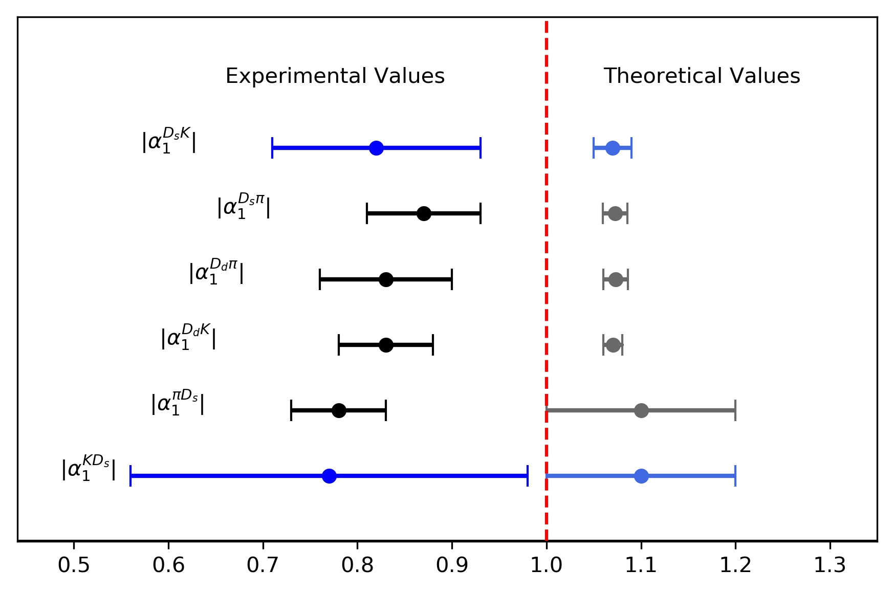
We complement our analysis, with a detailed look at other B(s)subscript๐ต๐‘ B_{(s)} decays with similar dynamics. Interestingly, we observe again a similar pattern, with the parameters following from the data being smaller than the theoretical values, as illustrated in Fig 2. Specifically, we find

$\displaystyle\bar{B}^{0}_{d}\rightarrow D_{d}^{+}K^{-}{\text{decay:}}\quad|a_{\rm 1}^{D_{d}K}|=0.83\pm 0.05,\quad{\text{differs at }}4.8\,\sigma{\text{ level, }}$
$\displaystyle\bar{B}^{0}_{d}\to D_{d}^{+}\pi^{-}{\text{decay:}}\quad|a_{1}^{D_{d}\pi}|=0.83\pm 0.07,\quad{\text{differs at }}3.3\,\sigma{\text{ level, }}$
Bยฏs0โ†’Ds+โ€‹ฯ€โˆ’โ€‹decay:|a1Dsโ€‹ฯ€|=0.87ยฑ0.06,differs atย โ€‹3.2โ€‹ฯƒโ€‹ย level,formulae-sequenceโ†’subscriptsuperscriptยฏ๐ต0๐‘ superscriptsubscript๐ท๐‘ superscript๐œ‹decay:superscriptsubscript๐‘Ž1subscript๐ท๐‘ ๐œ‹plus-or-minus0.870.06differs atย 3.2๐œŽย level,\displaystyle\bar{B}^{0}_{s}\to D_{s}^{+}\pi^{-}{\text{decay:}}\quad|a_{1}^{D_{s}\pi}|=0.87\pm 0.06,\quad{\text{differs at }}3.2\,\sigma{\text{ level, }}
Bยฏd0โ†’ฯ€+โ€‹Dsโˆ’โ€‹decay:|a1ฯ€โ€‹Ds|=0.78ยฑ0.05,differs atย โ€‹2.9โ€‹ฯƒโ€‹ย level.formulae-sequenceโ†’subscriptsuperscriptยฏ๐ต0๐‘‘superscript๐œ‹superscriptsubscript๐ท๐‘ decay:superscriptsubscript๐‘Ž1๐œ‹subscript๐ท๐‘ plus-or-minus0.780.05differs atย 2.9๐œŽย level.\displaystyle\bar{B}^{0}_{d}\to\pi^{+}D_{s}^{-}{\text{decay:}}\quad|a_{\rm 1}^{\pi D_{s}}|=0.78\pm 0.05,\quad{\text{differs at }}2.9\,\sigma{\text{ level. }}

This picture complements the intriguing $\gamma$ value. In view of these puzzling cases, we extend our analysis to include New Physics (NP) effects. Studies within physics beyond the SM can be found in [15, 16, 17], and NP effects in non-leptonic tree $B$ decays in [18, 19].

Refer to caption
Figure 2: Comparing the $|a_{1}|$ experimental and theoretical SM values for various decay processes.

4 Towards New Physics

Refer to caption
Refer to caption
Refer to caption
Figure 3: NP correlations in the $\bar{\varphi}$ $\varphi$ plane (left) and the $\bar{\rho}$ $\rho$ plane (center). We pick some points from the $\bar{\varphi}$ $\varphi$ plane and show the corresponding values in the $\bar{\rho}$ $\rho$ plane. The different colours come from different sign combinations of the $\rho\bar{\rho}$ term in the $\tan{\Delta\phi}$ expression. Uncertainties in the $\bar{\rho}$ $\rho$ plane (right).

If these puzzles are due to NP, it would have to enter at the amplitude level, as NP in mixing is included through the use of ฯ•ssubscriptitalic-ฯ•๐‘ \phi_{s} from data. Introducing the NP parameters

ฯยฏโ€‹eiโ€‹ฮดยฏโ€‹eiโ€‹ฯ†ยฏโ‰กAโ€‹(Bยฏs0โ†’Ds+โ€‹Kโˆ’)NP/Aโ€‹(Bยฏs0โ†’Ds+โ€‹Kโˆ’)SM,ยฏ๐œŒsuperscript๐‘’๐‘–ยฏ๐›ฟsuperscript๐‘’๐‘–ยฏ๐œ‘๐ดsubscriptโ†’subscriptsuperscriptยฏ๐ต0๐‘ superscriptsubscript๐ท๐‘ superscript๐พNP๐ดsubscriptโ†’subscriptsuperscriptยฏ๐ต0๐‘ superscriptsubscript๐ท๐‘ superscript๐พSM\bar{\rho}\,e^{i\bar{\delta}}e^{i\bar{\varphi}}\equiv{A(\bar{B}^{0}_{s}\rightarrow D_{s}^{+}K^{-})_{{\text{NP}}}}/{A(\bar{B}^{0}_{s}\rightarrow D_{s}^{+}K^{-})_{{\text{SM}}}}, (12)

with $\bar{\delta}$ and $\bar{\varphi}$ denoting the strong and weak NP phases, respectively (and similarly, ${\rho},{\delta},{\varphi}$ for the CP-conjugate case), we parametrise the amplitudes. Then, we can generalise the expression of the observables $\xi$ and $\bar{\xi}$ as well as the assumption $C+\overline{C}=0$ which was used by the LHCb Collaboration. The product can be generalised as follows [9, 10]:

ฮพร—ฮพยฏ=1โˆ’2โ€‹[C+Cยฏ(1+C)โ€‹(1+Cยฏ)]โ€‹eโˆ’iโ€‹[2โ€‹(ฯ•s+ฮณeff)],withฮณeffโ‰กฮณโˆ’12โ€‹(ฮ”โ€‹ฯ†+ฮ”โ€‹ฯ†ยฏ).formulae-sequence๐œ‰ยฏ๐œ‰12delimited-[]๐ถยฏ๐ถ1๐ถ1ยฏ๐ถsuperscript๐‘’๐‘–delimited-[]2subscriptitalic-ฯ•๐‘ subscript๐›พeffwithsubscript๐›พeff๐›พ12ฮ”๐œ‘ฮ”ยฏ๐œ‘\xi\times\bar{\xi}=\sqrt{1-2\left[\frac{C+\bar{C}}{\left(1+C\right)\left(1+\bar{C}\right)}\right]}e^{-i\left[2(\phi_{s}+\gamma_{\rm eff})\right]},\quad{\text{with}}\quad\gamma_{\rm eff}\equiv\gamma-\frac{1}{2}\left(\Delta\varphi+\Delta\bar{\varphi}\right). (13)

Here $\gamma$ enters with a shift due to the CP-violating NP phases, resulting in an effective angle $\gamma_{\rm eff}$. Setting the strong phases $\delta$ and $\bar{\delta}$ to 0, in agreement with factorization, we find

$$\tan{\Delta\phi}=\frac{\rho\sin{\phi}+\bar{\rho}\sin{\bar{\phi}}+\rho\bar{\rho}\sin{(\bar{\phi}+\phi)}}{1+\rho\cos{\phi}+\bar{\rho}\cos{\bar{\phi}}+\rho\bar{\rho}\cos{(\bar{\phi}+\phi)}}.$$ (14)

Using $\gamma=(70\pm 7)^{\circ}$, we obtain the numerical value $\Delta\varphi=-(61\pm 20)^{\circ}$.

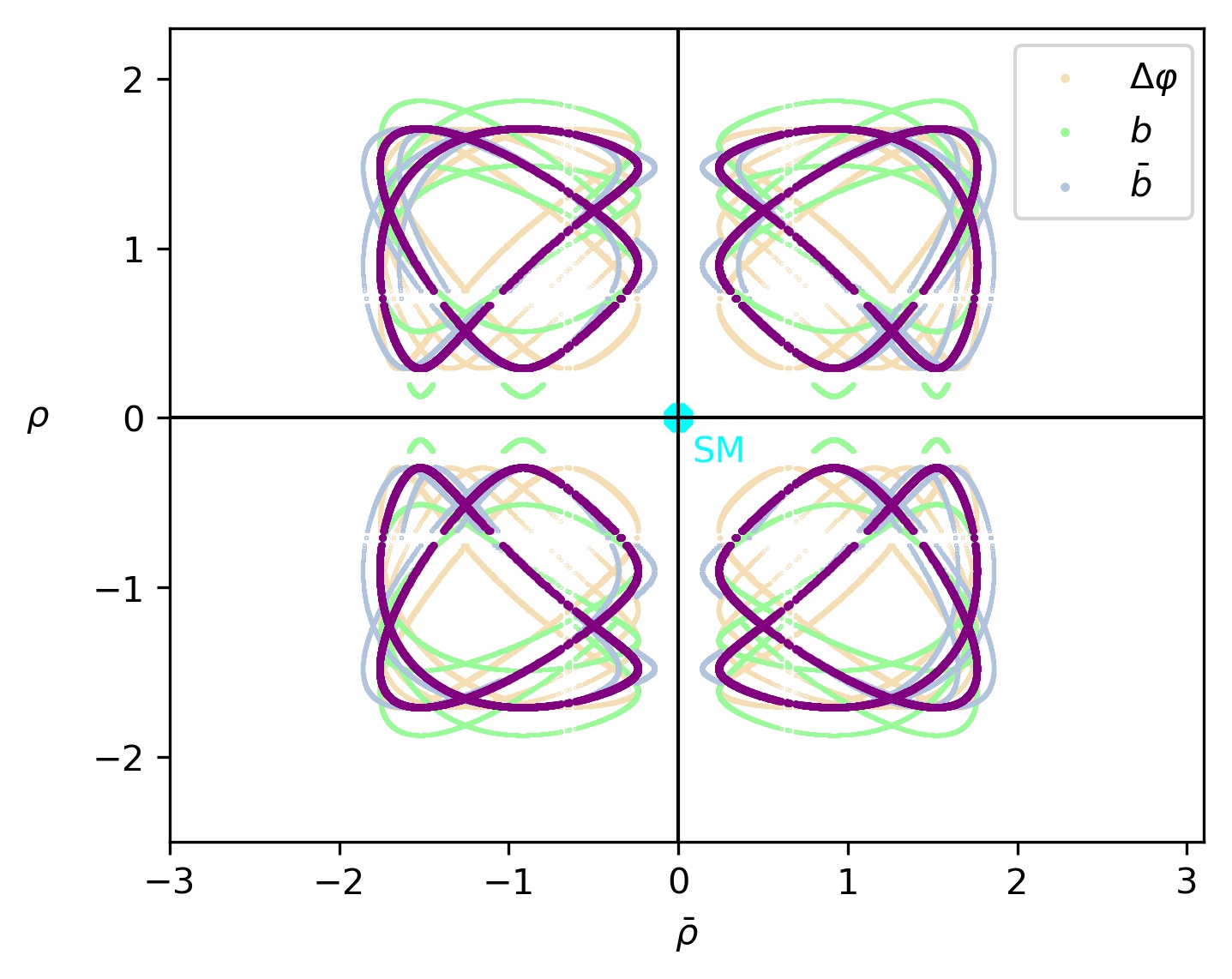
In the presence of NP, we use CP-averaged ratios $\langle R\rangle$, and introduce

$\displaystyle b$ =1+2โ€‹ฯโ€‹cosโกฮดโ€‹cosโกฯ•+ฯ2=โŸจRDs+โ€‹Kโˆ’โŸฉ6โ€‹ฯ€2โ€‹fK2โ€‹|Vuโ€‹s|2โ€‹|a1Dsโ€‹K|2โ€‹XDsโ€‹K=0.58ยฑ0.16,absent12๐œŒ๐›ฟitalic-ฯ•superscript๐œŒ2delimited-โŸจโŸฉsubscript๐‘…superscriptsubscript๐ท๐‘ superscript๐พ6superscript๐œ‹2superscriptsubscript๐‘“๐พ2superscriptsubscript๐‘‰๐‘ข๐‘ 2superscriptsuperscriptsubscript๐‘Ž1subscript๐ท๐‘ ๐พ2subscript๐‘‹subscript๐ท๐‘ ๐พplus-or-minus0.580.16\displaystyle=1+2\rho\cos{\delta}\cos{\phi}+\rho^{2}=\frac{\langle R_{D_{s}^{+}K^{-}}\rangle}{6\pi^{2}f_{K}^{2}|V_{us}|^{2}|a_{1}^{D_{s}K}|^{2}X_{D_{s}K}}=0.58\pm 0.16, (15)
$\displaystyle{\bar{b}}$ =1+2โ€‹ฯยฏโ€‹cosโกฮดยฏโ€‹cosโกฯ•ยฏ+ฯยฏ2=โŸจRK+โ€‹Dsโˆ’โŸฉ6โ€‹ฯ€2โ€‹fDs2โ€‹|Vcโ€‹s|2โ€‹|a1Kโ€‹Ds|2โ€‹XKโ€‹Ds=0.50ยฑ0.26,absent12ยฏ๐œŒยฏ๐›ฟยฏitalic-ฯ•superscriptยฏ๐œŒ2delimited-โŸจโŸฉsubscript๐‘…superscript๐พsuperscriptsubscript๐ท๐‘ 6superscript๐œ‹2superscriptsubscript๐‘“subscript๐ท๐‘ 2superscriptsubscript๐‘‰๐‘๐‘ 2superscriptsuperscriptsubscript๐‘Ž1๐พsubscript๐ท๐‘ 2subscript๐‘‹๐พsubscript๐ท๐‘ plus-or-minus0.500.26\displaystyle=1+2{\bar{\rho}}\cos{{\bar{\delta}}}\cos{{\bar{\phi}}}+{\bar{\rho}}^{2}=\frac{\langle R_{K^{+}D_{s}^{-}}\rangle}{6\pi^{2}f_{D_{s}}^{2}|V_{cs}|^{2}|a_{1}^{KD_{s}}|^{2}X_{KD_{s}}}=0.50\pm 0.26, (16)

allowing us to probe the NP parameters. In SM, these quantities are equal to 1.

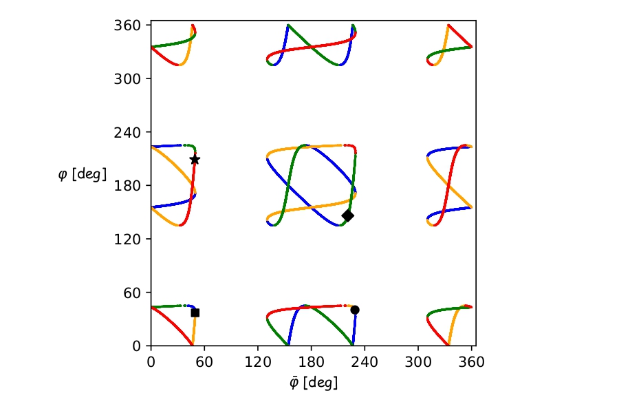
We would like to constrain the NP parameters through the data. Employing $b$ and $\bar{b}$, we may express $\rho$ and $\bar{\rho}$ in terms of $\varphi$ and $\bar{\varphi}$, respectively. Therefore, Eq.ย (14) allows us to calculate a correlation between ${\varphi}$ and $\bar{\varphi}$ (Fig.ย 3, left). Finally, using $\bar{\rho}(\bar{\varphi})$ and ${\rho}(\varphi)$, we may obtain the values of $\bar{\rho}$ and ${\rho}$ for a given value of $\bar{\varphi}$ and $\varphi$, respectively, thereby determining a correlation in the $\bar{\rho}$ $\rho$ plane (Fig.ย 3, central). We note that the SM point corresponding to the origin $(0,0)$ in the $\bar{\rho}$ $\rho$ plane is excluded. Values, in the regime around 0.5, could accommodate the central values of the current data, therefore resolving the puzzling patterns in the CP violation measurements as well as in the branching ratios. In the right plot of Fig.ย 3, we show the impact of the uncertainties of the input quantities $\bar{b}$, $b$ and $\Delta\varphi$, varying each one of them separately (lighter colours). We now observe that NP could accommodate the data with NP contributions as small as about $30\%$ of the SM amplitudes.

5 Conclusions

The Bs0โ†’Dsโˆ“โ€‹Kยฑโ†’subscriptsuperscript๐ต0๐‘ superscriptsubscript๐ท๐‘ minus-or-plussuperscript๐พplus-or-minusB^{0}_{s}\to D_{s}^{\mp}K^{\pm} system shows two puzzles: the CP violation measurements, reflected by the value of $\gamma$, and the branching ratios of the individual channels. We extract the parameters $a_{1}$ from the data in a clean way and we find consistent patterns in B(s)subscript๐ต๐‘ B_{(s)} decays with similar dynamics. In view of these puzzles, we have developed a model-independent strategy, generalising the analysis of the Bs0โ†’Dsโˆ“โ€‹Kยฑโ†’subscriptsuperscript๐ต0๐‘ superscriptsubscript๐ท๐‘ minus-or-plussuperscript๐พplus-or-minusB^{0}_{s}\to D_{s}^{\mp}K^{\pm} system in order to include effects from physics beyond the SM. Applying our formalism to the current data, we calculate correlations between the NP parameters and their CP-violating phases. Interestingly, we observe that both the CP violation and the branching ratio measurements can be described with NP contributions at the level of $30\%$ of the SM amplitudes. In the future high-precision era of $B$ physics, when much more data will be available, this strategy can be fully exploited. It will be exciting to see whether the tantalising question will be answered: Could new sources of CP violation be established?

References

  • [1] R.ย Aleksan, I.ย Dunietz and B.ย Kayser, Z. Phys. C 54 (1992), 653-660
  • [2] R.ย Fleischer, Nucl. Phys. B 671 (2003), 459-482
  • [3] K.ย De Bruyn et al., Nucl. Phys. B 868 (2013), 351-367
  • [4] R.ย Aaij et al. [LHCb], JHEP 03 (2018), 059
  • [5] Y.ย S.ย Amhis et al. [HFLAV], Eur. Phys. J. C 81, no.3, 226 (2021)
  • [6] P.ย A.ย Zyla et al. [Particle Data Group], PTEP 2020 (2020) no.8, 083C01
  • [7] R.ย Aaij et al. [LHCb], [arXiv:2110.02350 [hep-ex]].
  • [8] M.ย Z.ย Barel, K.ย De Bruyn, R.ย Fleischer and E.ย Malami, J. Phys. G 48 (2021) no.6, 065002
  • [9] R.ย Fleischer and E.ย Malami, [arXiv:2109.04950 [hep-ph]].
  • [10] R.ย Fleischer and E.ย Malami, [arXiv:2110.04240 [hep-ph]].
  • [11] M.ย Beneke, G.ย Buchalla, M.ย Neubert and C.ย T.ย Sachrajda, Nucl. Phys. B 591, 313-418 (2000)
  • [12] M.ย Bordone et al., Eur. Phys. J. C 80, no.10, 951 (2020)
  • [13] T.ย Huber, S.ย Krรคnkl and X.ย Q.ย Li, JHEP 09, 112 (2016)
  • [14] R.ย Fleischer, N.ย Serra and N.ย Tuning, Phys. Rev. D 83 (2011), 014017
  • [15] S.ย Iguro and T.ย Kitahara, Phys. Rev. D 102 (2020) no.7, 071701
  • [16] F.ย M.ย Cai, W.ย J.ย Deng, X.ย Q.ย Li and Y.ย D.ย Yang, JHEP 10 (2021), 235
  • [17] M.ย Bordone, A.ย Greljo and D.ย Marzocca, JHEP 08 (2021), 036
  • [18] J.ย Brod et al., Phys. Rev. D 92 (2015) no.3, 033002
  • [19] A.ย Lenz and G.ย Tetlalmatzi-Xolocotzi, JHEP 07 (2020), 177