Recovery of black hole mass from a single quasinormal mode
Gunther Uhlmann
Gunther Uhlmann
Department of Mathematics, University of Washington
and Institute for Advanced Study, the Hong Kong University of Science and Technology
gunther@math.washington.edu and Yiran Wang
Yiran Wang
Department of Mathematics, Emory University
yiran.wang@emory.edu
Abstract.
We study the determination of the mass of a de Sitter-Schwarzschild black hole from one quasinormal mode. We prove a local uniqueness result with a Hölder type stability estimate.
1. Introduction
The possibility of inferring black hole parameters from quasinormal modes (QNMs) has been explored in the physics literature, see Section 9 of the review paper [2]. For example, for slowly rotating black holes, Detweiler showed by numerical calculation in [7] that the wave parameters for the most damped mode are unique functions of the black hole parameters. Later, Echeverria in [10] investigated the stability issue. Since the success of gravitational wave interferometers, the topic has gained increasing attention, see e.g. [3]. One particular motivation for the study is to verify the black hole no hair theorem for which two QNMs are needed: one QNM is used to recover the black hole parameter and another QNM is used to test the theorem. We refer to [2, Section 9.7] for a review and [15] for the state of the art. Despite some convincing evidence, it seems that the theoretical justification is not complete. For example, most of the analysis in the literature is done for the fundamental modes corresponding to low angular momentum. However, it is generally not known which modes are excited and are extractable from the actual black hole ring down signals, see [3, 2]. In this short note, we aim to provide a mathematical justification of the recovery of black hole parameters from a single QNM.
We consider the model of a non-rotating de Sitter-Schwarzchild black hole :
(1)
where denotes the standard metric on and
(2)
Here, is the mass of the black hole and is the cosmological constant. They satisfy . are the two positive roots of which corresponds to horizons. Throughout the note, we assume that is known.
Consider the d’Alembertian on :
(3)
where and the positive laplacian on The stationary scattering is governed by the operator
(4)
see [19].
On with measure , is an essentially self-adjoint, non-negative operator, see [17].
Consider the resolvent
(5)
Here, we use as the spectral parameter and take to be the physical plane such that is bounded on for , according to the spectral theorem. Sá Barreto and Zworski demonstrated in [19, Proposition 2.1] that has a meromorphic continuation as operators from to from to with poles of finite rank. The poles of are called resonances. The fact that they are equivalent to the quasinormal modes defined by using Zerilli’s equation (see e.g. [6, 5]) are discussed in [19], see also [4, 17].
We denote the set of resonances by and set . We call a trivial resonance if for all For example, it is known that is a trivial resonance, see [17]. Trivial resonances can not be used to determine black hole parameters. Our main result is
Theorem 1.1.
Let and . For any not a trivial resonance, there exists (depending on ) such that for any with , if then
Moreover, if is sufficiently close to , then
for some and depending on .
We point out that resonances on are excluded in the theorem. There is a set of resonances on described by (22) which cannot be treated with our method, although their dependency on can be found explicitly. We do not investigate it further because such resonances are purely imaginary and they seem to be less relevant in practical cases, see for instance [15].
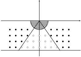
We also remark that for recovering black hole parameters, it is common to use only one or a few QNMs. This is very different from the usual inverse spectral/resonance problem for which the whole set is used to determine the parameters. In fact, there is a large literature on distribution of resonances for large angular momentum. For example, Theorem in [19] states that there exists such that for any there is an injective map from the set of pseudo-poles
in to such that all the poles in
are in the image of and for , we have
See Figure 1.
Figure 1. Resonances for de Sitter-Schwarzshild black holes. The black dots are resonances captured by Theorem in [19]. The hollow dots and resonances in the shaded region are not.
By looking at the sequence of resonances for large one
recovers . Similar results exist for rotating black holes, see for example [8].
Note that resonances sufficiently close to the lattice points cannot be trivial resonances. It is desirable to identify the trivial resonances, if there is any except There is some interesting recent result in [13] which shows the convergence of resonances to a set of for small masses. The numerical study [13, Fig. 6(b)] seems to indicate that such points are not trivial resonances.
Our proof of the theorem is based on analytic perturbation argument, by observing that the coefficients of the operator are analytic functions in . There are some resonance perturbation theories, see for instance Agmon [1], Howland [14], which are developed upon perturbation theory for eigenvalues, see for example [18]. Here, we use that has asymptotically hyperbolic structure near the two horizons to construct a parametrix modulo a trace-class error term, following Mazzeo and Melrose [16]. We then use the Fredholm determinant and its analyticity in to finish the proof. This approach has the benefit of not relying on the spherical symmetry of the black hole metric. It is clear from the proof that one can add metric or potential perturbations with suitable decay at the horizons to obtain a similar result to Theorem 1.1.
The note is organized as follows. We begin in Section 2 with a scattering problem to demonstrate the possibility of recovering parameters from a single resonance. In Section 3, we discuss the asymptotic hyperbolic structure and the analyticity. We construct the resolvent in Section 4 and finish the proof in Section 5.
2. An example: the potential barrier
In this section, we give an example of a scattering system depending on one parameter, for which a single resonance recovers the parameter. The example was actually used by Chandrasekhar and Detweiler in [6] to illustrate the concept of quasinormal mode.
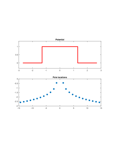
Consider
where is constant and is the rectangular barrier
See Figure 2. Note that the potential is characterized by . In this case, the scattering resonances can be defined as the poles of the scattering matrix. It is a standard exercise in scattering theory to find the scattering matrix. Let’s look at a wave traveling to the right, hit the potential and gets reflected and transmitted. In this case, the solution looks like
Here, is the refection coefficient and is the transmission coefficient. Similarly, we can consider a wave traveling to the left of the form
with the reflection, transmission coefficient respectively.
The scattering matrix is
By matching the solution and its derivatives at , we can find the coefficients as
where
Thus, the resonances are solutions of or equivalently
(6)
where Suppose we have such that . Then we can take modulus of (6) to find as
(7)
This shows that one can recover from one resonance.
Now we provide a numerical verification. We compute resonances using a Matlab code from [20] and identify using (7). It is important to note that the code from [20] does not calculate resonances by solving (7). Take . The potential and resonances are plotted in Figure 2. The numerical values of the four resonances nearest to the origin with positive real parts are
Using any of these resonances in (7), we find with a error.
Figure 2. A rectangular barrier and its resonances.
3. The asymptoically hyperbolic structure and analyticity
It is known that in (4) can be essentially viewed as perturbed Laplacians associated with some asymptotically hyperbolic metrics near . We follow the presentations in [17].
Let be a compact manifold of dimension with boundary . Let be a boundary defining function such that in , at , at
A metric on is called conformally compact if is a non-degenerate Riemannian metric on the closure . If in addition a constant, the metric is called asymptotically hyperbolic. In this case, the sectional curvature approaches along any curve towards , see [16, Lemma (2.5)]. There is a normal form of the metric near , see e.g. Graham [11]. In particular, there is a choice of boundary defining function such that in a neighborhood of , we can use local coordinate and get
We see that is a smooth function of on and analytic in . We set Here, we recall that
(9)
see page 6 of [19]. Thus are both analytic functions of
Now we write (4) as
(10)
For convenience, we denote with
Note that only vanishes at . We let be a boundary defining function defined through
(11)
Here, the smooth structure on is changed. Before, is a smooth boundary defining function near but now we think of as a smooth boundary defining function, see [19, Section 2].
By using , (10) becomes
(12)
Let be the metric defined in a neighborhood of given by
(13)
and let be the metric defined in a neighborhood of given by
(14)
These can be viewed as metric perturbations of the hyperbolic metrics
on with constant negative sectional curvature and respectively. Here, is the boundary defining function. Also, are even asymptotically hyperbolic metrics as defined in Guillarmou [12].
After some calculation see [17, Proposition 8.1], we conclude that there are two smooth functions such that
(15)
This shows the asymptotically hyperbolic structure of near
Consider the dependency of the operator on . Note that the manifold varies when varying . We change the notation from to . The dependency can be fixed by transforming to a fixed reference manifold. Let and let
be a diffeomorphism defined by with
Note that extends smoothly to .
Since are analytic functions of , and are also analytic in
Now, the pull back is a family of smooth boundary defining functions for . To see their dependency on , we write (2) as
where are two positive roots of and is the third negative root. Using (11) and on near , we have
(16)
where is defined through the last two lines. It is clear that is smooth in . Since for , we see that , hence , is analytic in Near , we have a similar form
(17)
From (13), (14), we see that the pull-back of the metrics are
(18)
near respectively. Here,
Let be the Lie algebra of smooth vector fields on vanishing at . In local coordinate near with being the boundary defining function, is generated by . The space of zero-differential operators of order on , denoted by is generated by fold products of vector fields in . From the analyticity of the diffeomorphism on , we see that the pull-back of to is a differential operator on with coefficients analytic in To see it belongs to with coefficients analytic in , we consider near for example near . We change the boundary defining function from to so . Then the metric in (18) becomes
which is a family of Riemannian metrics on analytic in
4. The resolvent construction
We obtain an approximation of in (5) following Mazzeo-Melrose [16]. In fact, we will find the resolvent of on . We will be using operators acting on half densities on . For convenience, we introduce an auxiliary Riemannian metric on which equals near respectively. Such a metric can be obtained by gluing near and some Riemannian metric in the interior of . The choice is clearly not unique and its dependency on is not important. We use to trivialize the (zero) one-density bundle , that is we take to be the volume form . The half-density bundle is
Let be a boundary defining function such that in local coordinates near , is expressed in form of (8). In this coordinate,
for some smooth function .
Now we consider acting on smooth sections in the following way
The resolvent is acting on in the same way.
The parametrix is constructed on the -blown-up space of as in [16]. Let be the diagonal of . Let which has two (disjoint) connected components.
As a set, the -blown-up space is
where denotes the inward pointing spherical bundle of . Let
(19)
be the blow-down map. Then is equipped with a topology and smooth structure of a manifold with corners for which is smooth. The manifold has the following boundary hyper-surfaces: the left and right faces and the front face . Since where the asymptotic behavior of the resolvent is different at each connected component, it is convenient to introduce
so , , see Figure 3.
The lifted diagonal is denoted by . has co-dimension two corners at the intersection of two of the boundary faces and co-dimension three corners given by the intersection of all the three faces. See Figure 3.
Figure 3. The 0-blown up space. The blown-up at the two components of are shown.
Now we introduce spaces of operator on . First, let be the space of conormal distributions of the bundle to and vanishing to infinite orders at . Here, it is understood that denotes the half-density bundle lifted from the one on by The corresponding class of pseudo-differential operators is denoted by . Next, let be the space of smooth vector fields on which are tangent to each of the boundary faces . Let be boundary defining functions. We set
(20)
Then define
Finally, define
Then we let be the space of operators on whose Schwartz kernel when lifted to belongs to .
We have the following result.
Proposition 4.1.
There is a family of operators with
(21)
analytic in and holomorphic in with
(22)
such that
(23)
Here, is trace class on for any Moreover, its Schwarz kernel is holomorphic in , and analytic in .
Proof.
For fixed , the construction of and and their holomorphy in is essentially contained in Proposition (7.4) of [16], which applies to the laplacian of asymptotically hyperbolic metrics. As argued in Proposition 2.2 of [19], the result applies to as the normal operator is elliptic. Because we argued in Section 3 that with coefficients analytic in , the construction in [16] produces analytic in The set comes from the poles of the resolvent of
see Lemma (6.15) of [16]. Here, denotes the positive laplacian of the standard hyperbolic metric. By rescaling the operator, we find the set
To find , it is convenient to work on . It suffices to consider the operators near respectively. Write . From [16, Theorem (7.1)], see also [12, Theorem 1.1], we know that the resolvent of
(24)
belongs to . Here, we followed [16] and used a different spectral parameter . Near , approaches . Comparing (24) with (12), we get
which gives . This gives , and can be found in the same way near
To see the trace class property, we recall a result [16, Lemma (5.24)]. The push forward of the space is
with the latter defined similarly to (20). Let be the Schwarz kernel of . As , we conclude that for we can write
where is analytic in . Near , using (13) and as local coordinate, we see that .
We get a similar expression near . Then we see that the integral is finite so is of trace class.
∎
Since is compact on , using analytic Fredholm theorem, we see that for any , is a family of bounded operators, meromorphic in . The poles (at least away from ) are the resonances. In fact, the resolvent is also meromorphic at , as clarified in [12].
Now we use the determinant of to analyze the poles. We recall that if is a trace class operator on a Hilbert space with eigenvalues with . Then the Fredholm determinant . See [9, Appendix B]. Also, is invertible if and only if is non-zero, see [9, Proposition B.28]. Therefore, the resonances of is contained in the zero set of
Using the argument in the end of [9, Section B.5], we conclude that is a function holomorphic in , and analytic in
Now we suppose is a resonance so . By the analyticity in , either is identically zero for all which means is a resonance for all , or is the only (discrete) zero locally. This proves the first claim of Theorem 1.1.
For the stability, we write for some and analytic in with . Now we set and get
We see that
Using the implicit function theorem, we get that is differentiable in a neighborhood of . Thus,
which implies
The authors thank Peter Hintz for his thorough reading of a previous version of the manuscript and for making very useful comments. GU was partly supported by NSF, a
Simons Fellowship, a Walker Family Endowed Professorship at UW and a Si-Yuan Professorship at IAS, HKUST.
References
[1] S. Agmon. A perturbation theory of resonances. Communications on Pure and Applied Mathematics 51.11‐12 (1998): 1255-1309.
[2] E. Berti, V. Cardoso, A. Starinets. Quasinormal modes of black holes and black branes. Classical and Quantum Gravity 26.16 (2009): 163001.
[3] E. Berti, V. Cardoso, C. Will. Gravitational-wave spectroscopy of massive black holes with the space interferometer LISA. Physical Review D 73.6 (2006): 064030.
[4] J.-F. Bony, D. Häfner. Decay and non-decay of the local energy for the wave equation on the de Sitter–Schwarzschild metric. Communications in Mathematical Physics 282.3 (2008): 697-719.
[5] S. Chandrasekhar. The mathematical theory of black holes. The International Series of Monographs on Physics, Volume 69, Clarendon Press, Oxford, UK (1983).
[6] S. Chandrasekhar, S. Detweiler. The quasi-normal modes of the Schwarzschild black hole. Proceedings of the Royal Society of London. A. Mathematical and Physical Sciences 344.1639 (1975): 441-452.
[7] S. Detweiler. Black holes and gravitational waves. III – The resonant frequencies of rotating holes. The Astrophysical Journal 239 (1980): 292-295.
[8] S. Dyatlov. Asymptotic distribution of quasi-normal modes for Kerr–de Sitter black holes. Annales Henri Poincaré. Vol. 13. No. 5. SP Birkhäuser Verlag Basel, 2012.
[9] S. Dyatlov, M. Zworski. Mathematical theory of scattering resonances. Vol. 200. American Mathematical Soc., 2019.
[10] F. Echeverria. Gravitational-wave measurements of the mass and angular momentum of a black hole. Physical Review D 40.10 (1989): 3194.
[11] R. Graham. Volume and area renormalizations for conformally compact Einstein metrics. Proceedings of the 19th Winter School. Circolo Matematico di Palermo, 2000.
[12] C. Guillarmou. Meromorphic properties of the resolvent on asymptotically hyperbolic manifolds. Duke Mathematical Journal 129.1 (2005): 1-37.
[13] P. Hintz, Y. Xie. Quasinormal modes of small Schwarzschild–de Sitter black holes. Journal of Mathematical Physics 63.1 (2022): 011509.
[14] J. Howland. Puiseux series for resonances at an embedded eigenvalue. Pacific Journal of Mathematics 55.1 (1974): 157-176.
[15] M. Isi, M. Giesler, W. Farr, M. Scheel, S. Teukolsky (2019). Testing the no-hair theorem with GW150914. Physical Review Letters, 123(11), 111102.
[16] R. Mazzeo, R. Melrose. Meromorphic extension of the resolvent on complete spaces with asymptotically constant negative curvature. Journal of Functional Analysis 75.2 (1987): 260-310.
[17] R. Melrose, A. Sá Barreto, A. Vasy. Analytic continuation and semiclassical resolvent estimates on asymptotically hyperbolic spaces. Communications in Partial Differential Equations 39.3 (2014): 452-511.
[18] M. Reed, B. Simon. Methods of modern mathematical physics IV: Analysis of operators. New York: Academic. (1978).
[19] A. Sá Barreto, M. Zworski. Distribution of resonances for spherical black holes. Mathematical Research Letters 4.1 (1997): 103-121.