On $(g-2)_{\mu}$ From Gauged $\mathrm{U}(1)_{X}$

Abstract

We investigate an economical explanation for the $(g-2)_{\mu}$ anomaly with a neutral vector boson from a spontaneously broken $\mathrm{U}(1)_{X}$ gauge symmetry. The Standard Model fermion content is minimally extended by 3 right-handed neutrinos. Using a battery of complementary constraints, we perform a thorough investigation of the renormalizable, quark flavor–universal, vector-like $\mathrm{U}(1)_{X}$ models, allowing for arbitrary kinetic mixing. Out of 419 models with integer charges not greater than ten, only 7 models are viable solutions, describing a narrow region in model space. These are either $L_{\mu}-L_{\tau}$ or models with a ratio of electron to baryon number close to $-2$. The key complementary constraints are from the searches for nonstandard neutrino interactions. Furthermore, we comment on the severe challenges to chiral $\mathrm{U}(1)_{X}$ solutions and show the severe constraints on a particularly promising such candidate.

1    Introduction

Measurements Bennett:2006fi ; Muong-2:2021ojo of the muon anomalous magnetic moment, $(g-2)_{\mu}$, are showing a combined $4.2\sigma$ deviation from the consensus Standard Model (SM) prediction Aoyama:2020ynm ; Colangelo:2020lcg ; aoyama:2012wk ; Aoyama:2019ryr ; czarnecki:2002nt ; gnendiger:2013pva ; davier:2017zfy ; keshavarzi:2018mgv ; colangelo:2018mtw ; hoferichter:2019gzf ; davier:2019can ; keshavarzi:2019abf ; kurz:2014wya ; melnikov:2003xd ; masjuan:2017tvw ; Colangelo:2017fiz ; hoferichter:2018kwz ; gerardin:2019vio ; bijnens:2019ghy ; colangelo:2019uex ; Blum:2019ugy ; colangelo:2014qya . This may be pointing to the existence of new physics (NP) coupling to muons. Such a possibility is especially intriguing in light of similar discrepancies in the $b\to s\mu^{+}\mu^{-}$ observables: angular distributions LHCb:2020lmf ; LHCb:2020gog ; branching ratios LHCb:2020zud ; LHCb:2021awg ; LHCb:2021vsc ; LHCb:2014cxe ; LHCb:2015wdu ; LHCb:2016ykl ; LHCb:2021zwz ; and the theoretically very clean lepton flavor universality (LFU) ratios, $R_{K^{(\ast)}}$ LHCb:2017avl ; LHCb:2021trn (for recent global fits see, e.g., Altmannshofer:2021qrr ; Geng:2021nhg ; Alguero:2021anc ; Hurth:2021nsi ; Ciuchini:2020gvn ). Global significance of the NP hypothesis in $b\to s\ell^{+}\ell^{-}$ decays, including the look-elsewhere effect, was estimated to be $4.3\sigma$ in Ref. Isidori:2021vtc .

Any NP model explaining the muon anomalies faces nontrivial experimental constraints. Especially stringent are the constraints from lepton flavor–violating (LFV) transitions, such as $\mu\to e\gamma$. While the $(g-2)_{\mu}$ anomaly requires a relatively low effective NP scale $\Lambda_{22}\simeq$15\text{\,}\mathrm{T}\mathrm{e}\mathrm{V}$$, the bound on the flavor-changing $\mu\to e\gamma$ transition requires $\Lambda_{12(21)}\gtrsim$3600\text{\,}\mathrm{T}\mathrm{e}\mathrm{V}$$ TheMEG:2016wtm . Viable NP explanations of $(g-2)_{\mu}$, therefore, must have highly suppressed LFV effects (as discussed in, e.g., Refs. Isidori:2021gqe ; Calibbi:2021qto ).

Strict flavor alignment between the dipole operator and the charged lepton mass matrix may well point to the existence of a new underlying symmetry, which we assume to be a spontaneously broken $\mathrm{U}(1)_{X}$ gauge group. The neutral gauge vector boson associated with the $\mathrm{U}(1)_{X}$ is then a candidate for an explanation of the $(g-2)_{\mu}$. One well-studied example of this scenarios is $\mathrm{U}(1)_{L_{\mu}\vbox{\hbox{\scalebox{0.6}[1.0]{$-$}}}L_{\tau}}$ He:1990pn ; He:1991qd ; Baek:2001kca ; Ma:2001md ; Harigaya:2013twa ; Altmannshofer:2014pba ; Altmannshofer:2019zhy ; Crivellin:2016ejn ; Crivellin:2015mga ; Crivellin:2018qmi ; Altmannshofer:2014cfa ; Altmannshofer:2015mqa ; Asai:2018ocx . The $\mathrm{U}(1)_{L_{\mu}\vbox{\hbox{\scalebox{0.6}[1.0]{$-$}}}L_{\tau}}$ gauge symmetry forces the dimension-4 charged lepton Yukawa interactions to be diagonal, ensuring an accidental $\mathrm{U}(1)^{3}$ lepton flavor symmetry. The $L_{\mu}-L_{\tau}$ gauge boson $X_{\mu}$ with mass $m_{X}\in[10,\,210]$ MeV and a coupling to muons in the range $g_{X}\in[0.4,\,1]\times 10^{-3}$ gives a one-loop contribution to $(g-2)_{\mu}$ of the right size to account for the experimental anomaly while not conflicting with any of other measurements Altmannshofer:2014pba ; Bauer:2018onh ; Escudero:2019gzq ; Amaral:2021rzw ; Greljo:2021npi .

There are two immediate questions pertaining to the anomaly-free $\mathrm{U}(1)_{X}$ gauge extensions of the SM:

1. Is $\mathrm{U}(1)_{L_{\mu}\vbox{\hbox{\scalebox{0.6}[1.0]{$-$}}}L_{\tau}}$ the only phenomenologically viable possibility that can explain the $(g-2)_{\mu}$ anomaly?

2. If there are alternative models, can these be experimentally disentangled from $\mathrm{U}(1)_{L_{\mu}\vbox{\hbox{\scalebox{0.6}[1.0]{$-$}}}L_{\tau}}$?

In this paper, we systematically explore the two questions, building on our previous work, Ref. Greljo:2021npi . The main result is that the only significant deviation of $L_{\mu}-L_{\tau}$ allowed by data is gauge groups where $L_{e}\simeq-2B$ and the kinetic mixing with the photon approximately cancels the electron charge. This conclusion is rather nontrivial since there exists an extensive list of precise experimental probes constraining complementary combinations of $\mathrm{U}(1)_{X}$ gauge boson couplings, resulting in a limited number of phenomenologically viable possibilities.

The main working assumptions for our analysis are i) the SM is minimally extended by three right-handed neutrinos and a flavor–non-universal $\mathrm{U}(1)_{X}$ gauge symmetry and ii) the theory is anomaly-free. The NP models also contain an SM singlet scalar field $\phi$ charged under $\mathrm{U}(1)_{X}$, whose vacuum expectation value (VEV) $v_{\phi}$ breaks the $\mathrm{U}(1)_{X}$. The solutions to the $(g-2)_{\mu}$ anomaly typically require $v_{\phi}$ around the electroweak scale if muons and $\phi$ carry ${\mathcal{O}}(1)$ $\mathrm{U}(1)_{X}$ gauge charges. The details about the source of $\mathrm{U}(1)_{X}$ symmetry breaking are not important for most of the phenomenology discussed in this paper, so our results do not change if a different SM-singlet condensate breaks $\mathrm{U}(1)_{X}$ (or several condensates). Actually, viable neutrino masses and mixings typically require more than one scalar field.

Requiring the ratios between (non-zero) $\mathrm{U}(1)_{X}$ charges for the chiral fermions to be at most ten gives roughly $21.5$ million inequivalent integer charge assignments, up to flavor permutation Allanach:2018vjg . We restrict our analysis to a subset of these, the 255 quark flavor–universal vector-like $\mathrm{U}(1)_{X}$ charge assignments Greljo:2021npi . Taking into account the flavor permutations among charged SM fermions this gives 419 phenomenologically distinct $\mathrm{U}(1)_{X}$ models. Here, we assumed that the sterile neutrinos are heavy enough so as not to affect the low-energy phenomenology, and, thus, different charge assignments for sterile neutrinos lead to the phenomenologically equivalent $\mathrm{U}(1)_{X}$ model in this counting. In Section 5, we furthermore comment on the 21 chiral $\mathrm{U}(1)_{X}$ charge assignments. The choice of quark flavor universality of $\mathrm{U}(1)_{X}$ charges is phenomenologically well motivated, since flavor–non-universal $\mathrm{U}(1)_{X}$ charges of quarks lead to dangerous flavor-changing neutral currents (FCNCs). As illustrated in Ref. Greljo:2021npi by a benchmark example, even for the second-safest option, a third-quark-family model with down-alignment, the CKM rotation induced up-sector FCNCs effectively rule out the parameter space preferred by $(g-2)_{\mu}$.

While quark flavor–universal models avoid FCNCs, they are still severely constrained through a combination of other measurements:

1. neutrino trident constraints Altmannshofer:2014pba ; Mishra:1991bv ; NuTeV:1999wlw ; Altmannshofer:2019zhy ;

2. electroweak precision observables ParticleDataGroup:2020ssz ; Haller:2018nnx ; ALEPH:2005ab ;

3. neutrino oscillation constraints on nonstandard neutrino interactions (NSI) Esteban:2018ppq ; Coloma:2020gfv ;

4. measurements of coherent neutrino scattering on nuclei Freedman:1973yd ; Drukier:1984vhf ; COHERENT:2017ipa ;

5. the Borexino measurement of the cross section for the elastic scattering of ⁷Be solar neutrinos on electrons Bellini:2011rx ; Borexino:2017rsf and other elastic neutrino-electron scattering experiments TEXONO:2009knm ; Beda:2009kx ; CHARM-II:1993phx ; CHARM-II:1994dzw ;

6. searches for new light resonances Ilten:2018crw ; Bauer:2018onh .

In Ref. Greljo:2021npi , we studied the implications of these measurements for several selected benchmarks. In this manuscript, we go well beyond the initial analysis of Ref. Greljo:2021npi and assess the constraints for the complete set of $419$ distinct vector-like $\mathrm{U}(1)_{X}$ models, focusing on the parameter space region relevant for explaining $(g-2)_{\mu}$. In several instances our phenomenological analysis applies to the complete class of quark flavor–universal vector-like charge assignment, even allowing for arbitrarily large charge assignments. We also comment on the phenomenology of chiral charge assignments, working out the details of the $\tilde{L}_{\mu-\tau}$ model in which the couplings of $X_{\mu}$ to electrons are purely axial, thus, eliminating the very strict constraints on NSI from neutrino oscillations.

In the bulk of the paper, the analysis is kept as general as possible. In particular, we do not impose any requirements regarding possible connections with the $b\to s\ell\ell$ anomalies. This does not mean that such connections do not exist. On the contrary, lepton flavor–non-universal $\mathrm{U}(1)_{X}$ gauge symmetries can further support solutions of the $B$-physics anomalies that rely on tree-level exchanges of leptoquarks (LQ). In general, TeV-scale LQs tend to excessively violate the accidental symmetries of the SM—baryon and individual lepton number symmetries—all of which are exquisitely tested experimentally. Charging the LQ under a flavor–non-universal $\mathrm{U}(1)_{X}$ gauge symmetry can reinstate the accidental symmetries while keeping the contributions to $B$-anomalies intact. Prominent examples of such mediators are the muoquarks Greljo:2021xmg ; Davighi:2020qqa ; Hambye:2017qix ; Davighi:2022qgb ; Heeck:2022znj , LQs charged under a $\mathrm{U}(1)_{X}$ such that they carry global muon and baryon numbers. Both of these remain accidentally conserved at dimension 4, as they are in the SM. Out of 255+21 quark flavor universal charge assignments, 252+21 satisfy the muoquark criteria for the scalar weak triplet mediator Greljo:2021npi .

The paper is organized as follows. In Section 2, we introduce the anomaly-free $\mathrm{U}(1)_{X}$ models and the parameter space relevant for $(g-2)_{\mu}$ bounded by cosmology ($m_{X}\gtrsim 10$ MeV) and perturbative unitarity ($m_{X}\lesssim 1$ TeV). Section 3 contains the discussion of the experimental constraints relevant for vector-like quark universal $\mathrm{U}(1)_{X}$ models. The phenomenological implications of these constraints are presented in Section 4: In Section 4.1, we use the neutrino trident production, combined with the $Z$-pole constraints, to set a robust upper limit on the $X$ boson mass ($m_{X}\lesssim 4$ GeV) for all renormalizable models introduced in Section 2. In Section 4.2, we perform a global analysis of experimental constraints and identify seven viable vector-like models that can explain the $(g-2)_{\mu}$ anomaly. Section 5 contains a brief discussion of chiral models and a detailed phenomenological analysis of the most promising example, the $\tilde{L}_{\mu-\tau}$ model. Possible connections with the $B$ anomalies are discussed in Section 6, while Section 7 contains conclusions. The details on the calculation of neutrino oscillation bounds are given in Appendix A, while Appendix B contains details on the construction of the global $\chi^{2}$ function used in the analysis.

2    Model framework

We start by reviewing the salient features of the gauged $\mathrm{U}(1)_{X}$ models and how these can address the $(g-2)_{\mu}$.

2.1    Field content and $\mathrm{U}(1)_{X}$ charges

The models we consider have the SM matter content extended by three sterile neutrinos $N_{i}$ while the SM gauge group is enlarged by an additional $\mathrm{U}(1)_{X}$ factor. After electroweak symmetry breaking (EWSB), the part of the Lagrangian relevant to the phenomenology at low energies ($m_{X}\ll m_{Z}$) is given by

$$\mathcal{L}\supset-\tfrac{1}{4}F_{\mu\nu}^{2}-\tfrac{1}{4}X_{\mu\nu}^{2}+\tfrac{1}{2}\varepsilon\,F_{\mu\nu}X^{\mu\nu}+\tfrac{1}{2}m_{X}^{2}X_{\mu}^{2}+eA_{\mu}J_{\scriptscriptstyle\mathrm{EM}}^{\mu}+g^{\prime}_{X}X_{\mu}J_{X}^{\mu},$$ (1)

where $F_{\mu\nu}$ and $X_{\mu\nu}$ are the electromagnetic and $\mathrm{U}(1)_{X}$ field strength tensors, $\varepsilon$ is the kinetic mixing parameter, $J^{\mu}_{{\scriptscriptstyle\mathrm{EM}}}$ the electromagnetic current, and $J_{X}^{\mu}=\sum_{f}x_{f}\overline{f}\gamma^{\mu}f$ the current associated with $\mathrm{U}(1)_{X}$, where $x_{f}$ are the $\mathrm{U}(1)_{X}$ charges for the chiral field $f$. The kinetic mixing term $\frac{\varepsilon}{2}\,F_{\mu\nu}X^{\mu\nu}$ can be removed by performing a non-unitary transformation of the Abelian gauge fields Holdom:1985ag , after which the $\mathrm{U}(1)_{X}$ Lagrangian is given by setting $\varepsilon\to 0$, $g^{\prime}_{X}\to g_{X}=g^{\prime}_{X}/\sqrt{1-\varepsilon^{2}}$ in Eq. (1) and shifting the charges according to

$$x_{f}\to x_{f}+\frac{\varepsilon}{\sqrt{1-\varepsilon^{2}}}\dfrac{e}{g_{X}}Q_{f}^{\scriptscriptstyle\mathrm{EM}}$$ (2)

in the expression for $J_{X}^{\mu}$ ($Q_{f}^{\scriptscriptstyle\mathrm{EM}}$ is the electric charge of the SM fermion $f$).

2.2    Charge assignments

The $\mathrm{U}(1)_{X}$ charges of quarks are assumed to be universal, such that the quark Yukawa interactions are given by the usual dimension-4 operators. Without loss of generality, we can set the $\mathrm{U}(1)_{X}$ charge of the SM Higgs to zero, $x_{H}=0$. This leaves 276 inequivalent charge assignment, not counting flavor permutations, with integer charges for the SM fields in the range from -10 to 10, as listed in Greljo:2021xmg . Shifting all the $x_{f}$ charges by a multiple of the hypercharge $Y_{f}$ gives physically equivalent models that would have $x_{H}\neq 0$, see Appendix A.1 of Ref. Greljo:2021xmg .

The above quark flavor–universal $\mathrm{U}(1)_{X}$ charge assignments fall into one of two categories. The 255 charge assignment in the vector category have vector-like $\mathrm{U}(1)_{X}$ charges for both the quarks and the charged leptons, $x_{L_{i}}=x_{E_{i}}$, $i=1,2,3$. The charged lepton masses are thus also generated via dimension-4 SM Yukawa interactions. Viable neutrino masses and mixings usually require additional $\mathrm{U}(1)_{X}$-breaking scalars (SM singlets), which lead to Majorana masses through $N_{i}N_{j}\phi_{ij}$ interactions. We assume that the sterile neutrinos are heavy enough that they are not relevant for the low energy phenomenology. Taking into account the flavor permutations of the vector-like $\mathrm{U}(1)_{X}$ charge assignments this leaves us with 419 phenomenologically distinct vector-like $\mathrm{U}(1)_{X}$ models. The possible charge assignments for the models in the vector category are given by Altmannshofer:2019xda ; Greljo:2021xmg

$$x_{f}=c_{e}{L_{e}}+c_{\mu}{L_{\mu}}+c_{\tau}{L_{\tau}}-\left(\tfrac{c_{e}+c_{\mu}+c_{\tau}}{3}\right){B}+\sum_{i}c_{N_{i}}L_{N_{i}},$$ (3)

where $\{B,{L_{e}},{L_{\mu}},{L_{\tau}}\}$ are the usual values of baryon and lepton numbers for the SM fermion $f$, while $L_{N_{i}}$ are the right-handed neutrino numbers ($N_{i}$ are not charged under $B,L_{\ell_{i}}$). The coefficients $\{c_{e},c_{\mu},c_{\tau},c_{N_{1}},c_{N_{2}},c_{N_{3}}\}$ in Eq. (3) need to satisfy the Diophantine equations Dobrescu:2020evn ; Allanach:2018vjg ($c_{e}+c_{\mu}+c_{\tau}=\sum_{i}c_{N_{i}}$ and $c_{e}^{3}+c_{\mu}^{3}+c_{\tau}^{3}=\sum_{i}c_{N_{i}}^{3}$) giving a 4 parameter family of models valid beyond the restriction to charges less than 10. In particular, there are valid solutions for any set of $c_{e},c_{\mu},c_{\tau}$: $c_{N_{i}}=(-c_{e},\,-c_{\mu},\,-c_{\tau})$. The parameterization in Eq. (3) will be exploited in Section 3.3 to asses NSI constraints on a large set of models.

The charge assignments $c_{N_{1}}=-c_{N_{2}}$, $c_{N_{3}}=c_{e,\mu,\tau}=0$ (and permutations thereof) correspond to the dark photon type solutions to $(g-2)_{\mu}$ Pospelov:2008zw . In this case, the $X$ couplings to the SM fermions are exclusively due to kinetic mixing with the photon—typically radiatively induced from $X$ interacting with some hidden sector particles also charged under the SM gauge group. This scenario has been ruled out as the solution of the $(g-2)_{\mu}$ anomaly, both when $X$ decays visibly NA482:2015wmo or invisibly NA64:2016oww ; BaBar:2017tiz , with the possible exception of a combined decay Mohlabeng:2019vrz .

There are additional 21 charge assignments for which there is no permutation such that $x_{L_{i}}=x_{E_{i}}$ for every $i=1,2,3$. These models constitute the chiral category and are listed in Section 2.2.2 of Greljo:2021xmg . We examine their phenomenology and possible relevance for $(g-2)_{\mu}$ separately, in Section 5. In chiral models at least some of the charged lepton Yukawa couplings to the Higgs are forbidden at dimension four, leading to Yukawa matrices of rank less than three. Hence, some of the charged lepton masses are generated through higher-dimension operators. We assume that these operators are either generated by integrating out vector-like fermions (which do not change the conditions for anomaly cancellation), or by integrating out heavy scalars. We discuss this in more detail for the $\tilde{L}_{\mu-\tau}$ model, including the phenomenological constraints, in Section 5.

2.3    Mater unification

Interestingly, some of the above $\mathrm{U}(1)_{X}$ extensions of the SM can be unified into a larger semi-simple gauge group at higher energies. As an example consider the vector category charge assignments with $x_{\ell_{i}}=x_{N_{i}}$. Ref. Davighi:2022qgb showed that in that case the $\mathrm{U}(1)_{Y}\times\mathrm{U}(1)_{X}$ can be unified into $\mathrm{SU}(2)_{R}\times\mathrm{U}(1)_{B-L}\times\mathrm{SU}(3)_{{\rm lep}}$. Starting from this semi-simple group the unification can proceed further (see Figure 1 of Ref. Davighi:2022qgb ).

2.4    Explanation of $(g-2)_{\mu}$

A massive vector $X_{\mu}$ coupling to muons with interaction

$$\mathcal{L}\supset g_{X}\,\overline{\mu}\,\not{X}(q_{V}-q_{A}\gamma_{5})\mu,$$ (4)

gives rise to a one-loop radiative correction to the anomalous magnetic moment of the muon:

$$\begin{split}\Delta a_{\mu}=\frac{g_{X}^{2}}{8\pi^{2}}\begin{dcases}q_{V}^{2}-2\,r_{\mu}^{2}\,q_{A}^{2},&m_{X}\ll m_{\mu},\\ \frac{2}{3}r_{\mu}^{2}\left[q_{V}^{2}-5\,q_{A}^{2}\right],&m_{X}\gg m_{\mu},\end{dcases}\,\end{split}$$ (5)

where $r_{\mu}=m_{\mu}/m_{X}$. For the full 1-loop expressions see, e.g., Refs. Jackiw:1972jz ; Jegerlehner:2009ry ; Greljo:2021npi . Correction (5) is of the right sign to explain the difference between the measured and predicted anomalous magnetic moment of the muon, $\Delta a_{\mu}=a^{\rm avg}_{\mu}-a^{\scriptscriptstyle\mathrm{SM}}_{\mu}=\left(251\pm 59\right)\times 10^{-11}$ Muong-2:2021ojo , if $X_{\mu}$ couples mainly vectorially to muons.

Requiring that $\Delta a_{\mu}$ is explained by a massive vector $X_{\mu}$ at one-loop order translates to an upper bound on the $\mathrm{U}(1)_{X}$ breaking VEV $\sqrt{2}\langle\phi\rangle=m_{X}/(g_{X}x_{\phi})<260\text{\leavevmode\nobreak\ GeV}\times(q_{V}/x_{\phi})$, which is saturated for $q_{A}=0$. Perturbative unitarity, $g_{X}q_{V}\leq\sqrt{4\pi}$, then implies an upper bound on the $X_{\mu}$ mass, $m_{X}\lesssim 1.0$ TeV (see Ref. Capdevilla:2021kcf for a more detailed discussion). This is a rather restrictive bound, the origin of which can be traced back to the fact that in the one-loop $X_{\mu}$ contribution to $(g-2)_{\mu}$, the required chirality flip necessarily occurs on the muon leg and, thus, is suppressed by the small muon mass.

2.5    Cosmology

A robust lower limit on the gauge boson mass $m_{X}$ follows from the agreement between observations of primordial light element abundances and the predictions within standard cosmology Big Bang Nucleosynthesis (BBN). The gauge coupling $g_{X}$ required to explain the $(g-2)_{\mu}$ anomaly is large enough that the gauge boson $X_{\mu}$ efficiently thermalises with the SM plasma in the early universe, i.e., for temperatures $T>m_{X}$. A light $X_{\mu}$ contributes with additional relativistic degrees of freedom during BBN, changing the predictions for light element abundances. This is avoided for $m_{X}\gtrsim 10$ MeV, in which case $X_{\mu}$ decays quickly, before the onset of BBN. The precise bound on $m_{X}$ was derived for the $\mathrm{U}(1)_{L_{\mu}-L_{\tau}}$ model in Ref. Kamada:2018zxi (see also Escudero:2019gzq ), and holds approximately also for all the other $\mathrm{U}(1)_{X}$ models considered here.

3    Experimental constraints

As a next step in the analysis, we discuss all the various constraints on the $\mathrm{U}(1)_{X}$ models. They include EW precision tests, a variety of neutrino interactions, and finally resonance searches.

3.1    Electroweak precision tests

After EWSB the $\mathrm{U}(1)_{X}$ gauge boson $X_{\mu}$ mixes both with the photon, $A_{\mu}$, and the $Z$ boson. The mixing with photon is important for low energy constraints, while the mixing with the $Z$ is severely constrained by the electroweak precision tests.

Electroweak symmetry breaking

In the models we consider, the source of the EWSB is the same as in the SM—the VEV of the SM Higgs. Above the electroweak scale the kinetic mixing Lagrangian between $X_{\mu}$ and the photon, Eq. (1), is replaced by the kinetic kinetic mixing between $X_{\mu}$ and $B_{\mu}$, parametrized by the parameter $\varepsilon_{Y}$:

$$\mathcal{L}\supset-\tfrac{1}{4}B_{\mu\nu}^{2}-\tfrac{1}{4}X^{2}_{0,\mu\nu}+\tfrac{1}{2}\varepsilon_{Y}\,B_{\mu\nu}X_{0}^{\mu\nu}-\tfrac{1}{4}(W_{\mu\nu}^{a})^{2}+|D_{\mu}H|^{2}+\tfrac{1}{2}m_{X_{0}}^{2}X_{0,\mu}^{2},$$ (6)

where $D_{\mu}H=(\partial_{\mu}+ig_{X}^{\prime}x_{H}X_{0,\mu})H$. In writing the above Lagrangian we remain agnostic about the origin of the $X$ boson mass. The mass term $m_{X_{0}}$ could be due to a VEV of a single SM singlet scalar or due to a more complicated condensate in the SM singlet sector.

The $\mathrm{U}(1)_{X}$ charge of the SM Higgs, $x_{H}$, can be absorbed in the other parameters by performing the shift

$$\big{\{}g^{\prime}_{X},\,\varepsilon_{Y}\big{\}}\longrightarrow\frac{1}{\sqrt{1+2\varepsilon_{Y}\,\xi+\xi^{2}}}\big{\{}g^{\prime}_{X},\,\varepsilon_{Y}+\xi\big{\}},$$ (7)

where $\xi=2x_{H}{g^{\prime}_{X}}/{g_{1}}$. This shift changes the charges $x_{f}$ of the matter fields, $f$, by

$$x_{f}\longrightarrow x_{f}-2x_{H}Y_{f},$$ (8)

with $Y_{f}$ the hypercharge of fermion $f$. Without loss of generality, we can, therefore, take $x_{H}=0$, which is what we will assume from now on.

Expressing $B_{\mu}$ and $W_{\mu}^{3}$ in Eq. (6) in terms of the photon, $A_{\mu}$, and the $Z$ boson field, $Z_{\mu}$, gives the kinetic mixing Lagrangian after EWSB:

$$\begin{split}\mathcal{L}\supset&-\tfrac{1}{4}\big{(}A_{\mu\nu}^{2}+X^{2}_{0,\mu\nu}+Z_{0,\mu\nu}^{2}\big{)}+\tfrac{1}{2}m_{Z_{0}}^{2}\!Z_{0,\mu}^{2}+\tfrac{1}{2}m_{X_{0}}^{2}X_{0,\mu}^{2}\\ &+\tfrac{1}{2}\varepsilon_{Y}\!\big{(}c_{w}A_{\mu\nu}-s_{w}Z_{0,\mu\nu}\big{)}X_{0}^{\mu\nu},\end{split}$$ (9)

where $m_{Z_{0}}=g_{Z}\langle H\rangle/\sqrt{2}$ is the SM $Z$ mass. In Eq. (9) we do not write down the terms involving dynamical Higgs field. We also used the shorthand notation $s_{w}=\sin\theta_{w}$, $c_{w}=\cos\theta_{w}$, and $t_{w}=\tan\theta_{w}$, where $\theta_{w}$ is the weak mixing angle.

A simultaneous diagonalization of the kinetic and mass terms is achieved by a combination of a non-unitary field redefinition and a rotation,

$$\begin{pmatrix}A^{\mu}\\ Z_{0}^{\mu}\\ X_{0}^{\mu}\end{pmatrix}\!=\begin{pmatrix}1&\phantom{1/r_{\varepsilon}}&c_{w}\hat{\varepsilon}_{Y}\\ &1&\vbox{\hbox{\scalebox{0.6}[1.0]{$-$}}}s_{w}\hat{\varepsilon}_{Y}\\ &&\Delta_{\varepsilon}\\ \end{pmatrix}\!\begin{pmatrix}1&&\\ &c_{\theta}&s_{\theta}\\ &\vbox{\hbox{\scalebox{0.6}[1.0]{$-$}}}s_{\theta}&c_{\theta}\\ \end{pmatrix}\!\begin{pmatrix}A^{\mu}\\ Z^{\mu}\\ X^{\mu}\end{pmatrix},$$ (10)

where $\Delta_{\varepsilon}^{2}=1/(1-\varepsilon_{Y}^{2})$. The mixing angle $\theta$ between $Z$ and $X$ is given by

$$t_{\theta}=\begin{dcases}\frac{s_{w}\hat{\varepsilon}_{Y}}{1-r_{X}^{2}},&|s_{w}\hat{\varepsilon}_{Y}|<|1-r_{X}^{2}|,\\ \frac{1-r_{X}^{2}}{s_{w}\hat{\varepsilon}_{Y}},&|s_{w}\hat{\varepsilon}_{Y}|>|1-r_{X}^{2}|,\end{dcases}$$ (11)

where

$$r_{X}=\dfrac{m_{X}}{m_{Z_{0}}},\quad\mathrm{and}\quad\hat{\varepsilon}_{Y}=\dfrac{\varepsilon_{Y}}{\sqrt{1-\varepsilon_{Y}^{2}}},$$ (12)

with $m_{X}$ the physical $X$ boson mass.

The diagonalization of the gauge fields changes their effective currents. From Eq. (10), we find that

$$\mathcal{L}\supset eJ_{A}^{\mu}A_{\mu}+g_{Z}J_{Z}^{\mu}Z_{0,\mu}+g_{X}^{\prime}J_{X}^{\mu}X_{0,\mu}=eJ_{A}^{\mu}A_{\mu}+g_{Z}J_{Z,{\rm eff}}^{\mu}Z_{\mu}+g_{X}J_{X,{\rm eff}}^{\mu}X_{\mu},$$ (13)

with

$$J_{Z,{\rm eff}}^{\mu} =c_{\theta}\!\left[J^{\mu}_{Z}-{c_{w}\,t_{\theta}\,\hat{\varepsilon}_{Y}}J_{Y}^{\mu}-t_{\theta}\dfrac{g_{X}}{g_{Z}}J_{X}^{\mu}\right]\!,$$ (14)

$$J_{X,{\rm eff}}^{\mu} =J_{X}^{\mu}+c_{w}\,c_{\theta}\hat{\varepsilon}_{Y}\dfrac{e}{g_{X}}J_{A}^{\mu}+c_{\theta}\dfrac{\,g_{Z}}{g_{X}}\!\left(t_{\theta}-s_{w}\hat{\varepsilon}_{Y}\right)\!J_{Z}^{\mu},$$ (15)

where $g_{X}=c_{\theta}\Delta_{\varepsilon}g^{\prime}_{X}$ is the physical $X$ gauge coupling.

$Z$ mass constraint

The kinetic mixing between $X_{\mu}$ and $B_{\mu}$ introduces a mass mixing between $Z$ and $X$ gauge bosons, resulting in a shift of the physical $Z$ mass $m_{Z}$ and corrections to $Z$ couplings to SM fermions. While a global fit to the electroweak precision data would be required to capture all the resulting experimental constraints on $X_{\mu}$–$B_{\mu}$ mixing, it suffices for our purposes to consider just the $T$ parameter (marginalized over other electroweak observables), mainly because the measurements of SM fermion couplings to $Z$ have larger relative errors, see also discussion in Ref. Efrati:2015eaa , as well as Refs. Babu:1996vt ; Babu:1997st ; Cassel:2009pu ; Curtin:2014cca , and Section 3.1 below.

We find that

$$\rho_{0}=\frac{m_{Z,{\scriptscriptstyle\mathrm{SM}}}^{2}}{m_{Z,\mathrm{obs}}^{2}}\simeq\frac{m_{Z_{0}}^{2}}{m_{Z}^{2}}=\dfrac{1-r_{X}^{2}}{1-r_{X}^{2}+s_{w}^{2}\hat{\varepsilon}_{Y}^{2}},$$ (16)

where $m_{Z,{\scriptscriptstyle\mathrm{SM}}}$ is the SM prediction for the $Z$ mass (from the $W$ mass including radiative corrections), whereas $m_{Z,\mathrm{obs}}$ is the measured $Z$ mass so that in the SM $\rho_{0}=1$. Since we are interested in the NP constraints, we can use the tree-level relations, giving the second (approximate) equality. $\rho_{0}$ is related to the oblique parameter $T$ through $\rho_{0}-1=1/(1-\hat{\alpha}(m_{Z})T)-1\simeq\hat{\alpha}(m_{Z})T$, where experimentally from the electroweak fit $T=$0.03\pm 0.12$$, when the $S,U$ parameters are allowed to float freely ParticleDataGroup:2020ssz (see also Baak:2014ora ). The $Z$ mass shift in our model results in

$$T=-\dfrac{1}{\alpha(m_{Z})}\dfrac{s_{w}^{2}\hat{\varepsilon}_{Y}^{2}}{1-r_{X}^{2}+s_{w}^{2}\hat{\varepsilon}_{Y}^{2}}.$$ (17)

In the limit of small $X$ mass and small kinetic mixing parameter, we have

$$T=-\dfrac{s_{w}^{2}}{\alpha}\varepsilon^{2}_{Y}\left[1+\mathcal{O}\big{(}\varepsilon_{Y}^{2},\,m_{X}^{2}/m_{Z}^{2}\big{)}^{2}\right]\simeq-30\,\varepsilon^{2}_{Y}.$$ (18)

This provides a relatively weak bound for the region of light $X$ masses ($m_{X}<2m_{\mu}$)

$$|\varepsilon_{Y}|<0.076,$$ (19)

well above the typical expectation $\varepsilon_{Y}\sim{\mathcal{O}}(eg_{X}/16\pi^{2})$ for radiatively induced kinetic mixing. Nevertheless, the $T$ parameter bound in Eq. (19) is phenomenologically quite important, since it does not allow for arbitrarily large kinetic mixings. Combined with constraints from neutrino trident production, it translates to a model-independent requirement that $X$ needs to be lighter than a few GeV (see Section 3.2 for details).

For $X$ masses comparable to $m_{Z}$, the bound in Eq. (19) becomes more stringent and then progressively weaker for $m_{X}\gg m_{Z}$. Throughout this region, the mixing angle $\theta$ between $X$ and $Z$ is given by the upper expression in Eq. (11), except for the very small region where $X$ and $Z$ are almost mass degenerate, such that $|s_{w}\hat{\varepsilon}_{Y}|>|1-r_{X}^{2}|$. In this mass degenerate regime, the constraint on the $T$ parameter leads to

$$|s_{w}\hat{\varepsilon}_{Y}|<\frac{\alpha|T|}{1-\alpha|T|}\implies|\varepsilon_{Y}|<$4.7\text{\times}{10}^{-3}$.$$ (20)

As anticipated, in this region, the constraint on $|\varepsilon_{Y}|$ is significantly more stringent than it is for the light $X$ mass limit, Eq. (19). From the $T$ bound, it follows that this case is only relevant for $|1-r_{X}^{2}|<$2.2\text{\times}{10}^{-3}$$, i.e., when the $X$ and $Z$ are degenerate to within $0.2\%$.

Lepton universality in $Z$ decays

The mixing between $X$ and $Z$ also results in non-universal $Z$ boson couplings to the SM leptons, Eq. (14), which were measured to high precision at LEP ALEPH:2005ab . We expect the strongest constraint to come from the lepton flavor universality ratio for first two generations of leptons ALEPH:2005ab ,

$$R_{\mu e}=\dfrac{\Gamma(Z\to\mu^{+}\mu^{-})}{\Gamma(Z\to e^{+}e^{-})}=$1.0009\pm 0.0028$.$$ (21)

Using Eq. (14), we obtain

$$\delta R_{\mu e}\simeq\dfrac{4}{1-4s_{w}^{2}+8s_{w}^{4}}\dfrac{t_{\theta}g_{X}}{g_{Z}}\Big{[}x_{L_{2}}-x_{L_{1}}+2s_{w}^{2}(x_{L_{1}}+x_{E_{1}}-x_{L_{2}}-x_{E_{2}})\Big{]}.$$ (22)

for the leading new physics contributions to flavor universality ratio. This bound is more model-dependent than the $T$ bound, since it depends on the $\mathrm{U}(1)_{X}$ charges of the leptons that change from one $\mathrm{U}(1)_{X}$ model to another. To be completely consistent, one would in principle have to perform a global electroweak fit for every $\mathrm{U}(1)_{X}$ model. However, we estimate the typical non-universal effects to be sub-leading and, thus, their inclusion would only marginally improve on the constraint obtained from the $T$ parameter in Section 3.1.

Effective $X$ current

After EWSB the effective couplings of $X$ boson (the mass eigenstate mostly composed of $X_{0}$) are encoded in the effective current $J_{X,{\rm eff}}$, Eq. (15). In the limit $|s_{w}\hat{\varepsilon}_{Y}|<|1-r_{X}^{2}|$ the current takes a simpler form:

$$J_{X,\mathrm{eff}}^{\mu}=J_{X}^{\mu}+c_{\theta}s_{w}\hat{\varepsilon}_{Y}\frac{g_{Z}}{g_{X}}\left[c_{w}^{2}J_{A}^{\mu}+\frac{r_{X}^{2}}{1-r_{X}^{2}}J_{Z}^{\mu}\right].\\$$ (23)

For small masses, $m_{X}\ll m_{Z}$, the last term is power suppressed and we find agreement with the low-energy description of $X$ mixing with the photon, given in Section 2.1. A comparison with Eq. (2) yields

$$\varepsilon=c_{w}\,\varepsilon_{Y}.$$ (24)

3.2    Neutrino trident production

The $\Delta a_{\mu}$ anomaly points to a vector boson in the mass range $10$ MeV $\lesssim m_{X}\lesssim 1$ TeV. The viable mass window is set by cosmology (lower limit, see Section 2.5) and perturbative unitarity (upper limit, see Section 2.4). An efficient complementary constraint, which cuts significantly into this parameter range, is due to limits on nonstandard neutrino trident production, i.e., the scattering of a muon neutrino on a nucleus, producing a pair of charged muons, $\nu_{\mu}N\to\nu_{\mu}N\mu^{+}\mu^{-}$. In combination with the constraints from the electroweak $T$ parameter, Section 3.1, it limits the $X$ mass to $m_{X}\lesssim 4$ GeV, as we show below.

Neutrino induced production of a $\mu^{+}\mu^{-}$ pair in the Coulomb field of a heavy nucleus is a rare electroweak process in the SM. In $\mathrm{U}(1)_{X}$ models, there is an additional tree-level contribution from the diagram with an $X_{\mu}$ gauge boson exchanged between $\nu_{\mu}$ and $\mu$ legs. The strongest bound on this contribution is due to the CCFR experiment Mishra:1991bv , which reported the measurement

$$\frac{\sigma_{\scriptscriptstyle\mathrm{CCFR}}}{\sigma_{\scriptscriptstyle\mathrm{SM}}}=0.82\pm 0.28\leavevmode\nobreak\ .$$ (25)

for a trident cross section normalized to the SM prediction. This imposes constraints on the vector and axial vector couplings of $X_{\mu}$ to muons. We derive the resulting bounds on the gauge coupling $g_{X}$ as a function of $m_{X}$ for the $\mathrm{U}(1)_{X}$ models using the public code of Ref. Altmannshofer:2019zhy (further details can be found in Ref. Greljo:2021npi ). In the EFT region, $m_{X}\gtrsim$1\text{\,}\mathrm{G}\mathrm{e}\mathrm{V}$$, this bound is approximated by Altmannshofer:2019zhy

$$\frac{\sigma_{\scriptscriptstyle\mathrm{CCFR}}}{\sigma_{\scriptscriptstyle\mathrm{SM}}}\simeq\frac{\big{(}\tfrac{1}{2}+2s_{w}^{2}+C_{V}\big{)}^{2}+1.13\big{(}\tfrac{1}{2}+C_{A}\big{)}^{2}}{\big{(}\tfrac{1}{2}+2s_{w}^{2}\big{)}^{2}+1.13/4},$$ (26)

where

$$C_{V,A}=\frac{g_{X}^{2}}{\sqrt{2}G_{F}m_{X}^{2}}q_{\nu}q_{V,A}$$ (27)

are the normalized NP coefficients of the effective 4-fermion interactions between muon neutrinos and vector and axial muons, respectively. $G_{F}$ is the Fermi constant, controlling the overall strength of the SM contribution, while $q_{V,A}$ and $q_{\nu}$ are the effective $\mathrm{U}(1)_{X}$ vector and axial charges of muons and the charge of muon neutrinos, respectively (cf. Eq. (4)):

$$\mathcal{L}\supset g_{X}\,\overline{\mu}\,\not{X}(q_{V}-q_{A}\gamma_{5})\mu+g_{X}\,\overline{\nu}_{\mu}\,q_{\nu}\not{X}P_{L}\nu_{\mu}.$$ (28)

3.3    Neutrino oscillations and coherent elastic neutrino-nucleus scattering

Beyond the trident production, discussed in Section 3.2, the $\mathrm{U}(1)_{X}$ solutions to the $(g-2)_{\mu}$ anomaly also lead to two other types of nonstandard neutrino interactions (NSI): the modified matter effects in neutrino oscillations and the additional contributions to coherent elastic neutrino–nucleus scattering.

The matter effects in neutrino oscillations are given by the forward scattering amplitude, i.e., at zero momentum transfer. Accordingly, the NSI contributions are well described by the EFT Lagrangian ($f=\{e,p,n\}$) Wolfenstein:1977ue ; Mikheyev:1985zog ; Antusch:2008tz ; Coloma:2020gfv ,

$$\mathcal{L}_{\scriptscriptstyle\mathrm{NSI}}=-{2\sqrt{2}}{G_{F}}\sum_{f,\alpha\beta}\varepsilon_{\alpha\beta}^{f}(\overline{f}\gamma_{\mu}f)(\overline{\nu}_{\alpha}P_{\mathrm{L}}\nu_{\beta})\leavevmode\nobreak\ ,$$ (29)

even for $m_{X}$ well below the mass window of interest, $m_{X}\gtrsim 10$ MeV. In our setup, the NSI are generated at tree level by integrating out the gauge field $X_{\mu}$. We use the results of a global EFT fit to the neutrino oscillations data Esteban:2018ppq ; Coloma:2020gfv ; Heeck:2018nzc to set constraints on $X_{\mu}$ couplings to $u$ and $d$ quarks and to electrons (cf. App. A). The constraints are numerically important for the $(g-2)_{\mu}$ compatible parameter space. For instance, the upper limit on $g_{X}/m_{X}$ from neutrino oscillations rules out $\mathrm{U}(1)_{B-3L_{\mu}}$ as a possible solution to the $(g-2)_{\mu}$ anomaly, despite relatively small couplings to quarks, $x_{q}/x_{\mu}\ll 1$ (see Fig. 3 in Ref. Greljo:2021npi ).

The bounds on NSI from neutrino oscillations, Eq. (29), are sensitive to the average $\mathrm{U}(1)_{X}$ charge of the material the neutrinos propagate through, either the Earth’s mantel and core or the sun. Among other implications, this means that the value of the kinetic mixing $\varepsilon$ has no effect on the neutrino oscillation bounds, since the matter is electrically neutral. The bounds from neutrino oscillations are relaxed for a particular set of $\mathrm{U}(1)_{X}$ models, such as $B-2L_{e}-L_{\tau}$ and $B-2L_{e}-L_{\mu}$, for which the average $\mathrm{U}(1)_{X}$ charge of normal matter is almost zero (nuclei have, on average, roughly as many protons as neutrons, i.e., $B\simeq 2L_{e}$ for normal matter).

A complementary set of constraints on NSI is due to coherent elastic neutrino–nucleus scattering Freedman:1973yd ; Drukier:1984vhf , which was observed by the COHERENT experiment COHERENT:2017ipa . In this case, the EFT description in Eq. (29) is not valid for the full range of $X$ masses of interest to our analysis, $10$ MeV $\lesssim m_{X}\lesssim 4$ GeV. Following Ref. Greljo:2021npi , we instead keep $X_{\mu}$ as a dynamical field when setting the bounds on $g_{X}$, using the likelihood from Ref. Denton:2020hop .

3.4    Elastic neutrino-electron scattering

The Borexino experiment measured the cross section for elastic scattering of solar neutrinos on electrons Bellini:2011rx ; Borexino:2017rsf , which constrains possible new $X_{\mu}$ mediated interactions between neutrinos and electrons. The strongest bound on light vector boson interactions is obtained from ${}^{7}\mathrm{Be}$ neutrinos, which have an energy of $862\text{\,}\mathrm{k}\mathrm{e}\mathrm{V}$. The direct $X$ coupling to electrons can significantly change the scattering cross section of solar neutrinos, especially due to many $\mathrm{U}(1)_{X}$ models having large couplings to muon and tau neutrinos. The $\nu_{\mu}$ and $\nu_{\tau}$ neutrino flavors are present in the solar flux on Earth, since the initial $\nu_{e}$ neutrinos oscillate during propagation from the Sun. We follow the analysis of Ref. Altmannshofer:2019zhy to place bounds on $g_{X}$ while requiring that the scattering cross section remains within $2\sigma$ of the measurement.

The reactor experiments TEXONO TEXONO:2009knm and GEMMA Beda:2009kx measured the related cross section for elastic scattering of electron anti-neutrinos on electrons, while the high-energy beam experiment CHARM-II at CERN measured the cross sections for elastic $\nu_{\mu}e^{-}$ and $\bar{\nu}_{\mu}e^{-}$ scattering CHARM-II:1993phx ; CHARM-II:1994dzw . These bounds can be as relevant as Borexino and will be discussed in the context of the chiral $\tilde{L}_{\mu-\tau}$ model in Section 5, where the electron coupling is purely axial avoiding bounds from NSI oscillations.

3.5    Resonance searches

Several intensity-frontier collider experiments Ilten:2018crw ; Bauer:2018onh have directly searched for a production of a vector resonance $X$ in the mass range of interest, $10\,\text{MeV}\lesssim m_{X}\lesssim 4\,\text{GeV}$.

In a fixed target experiment such as NA64 Banerjee:2019pds , the vector boson is produced via bremsstrahlung process $eN\to eNX$, where $N$ is a nucleus. The most relevant decay mode is $X\to\mathrm{invisible}$, which is typically dominant below the dimuon threshold. The events are reconstructed from the missing energy measurements. The NA64 search Banerjee:2019pds constrains the $X$ couplings to electrons, which enter the prediction for the $X$ production rates. Future NA64$\mu$ Gninenko:2018ter and $M^{3}$ Kahn:2018cqs experiments will feature muons in the incoming beam and will have the potential to cover the entire parameter space of the $L_{\mu}-L_{\tau}$ model, see Fig. 2 in Ref. Greljo:2021npi . The fixed target experiments are effective only for $m_{X}\lesssim 1$ GeV.

Another important set of direct searches was performed at $B$-factories and probed $X$ masses up to $10$ GeV. The BaBar search for $e^{+}e^{-}\to\mu^{+}\mu^{-}X$ in the $4\mu$ final state BaBar:2016sci (labeled in figures as BaBar 2016) sets fairly stringent constraints above the dimuon threshold. BaBar also searched for a radiative return process $e^{+}e^{-}\to\gamma X$ with $X$ decaying to $e^{+}e^{-}$ or $\mu^{+}\mu^{-}$ BaBar:2014zli (BaBar 2014 and LHCb) or to invisible BaBar:2017tiz (BaBar 2017). The LHC searches extend the exclusion to even larger $X$ masses, such as the LHCb search for $X\to\mu^{+}\mu^{-}$ LHCb:2017trq ; LHCb:2019vmc and the CMS search for $Z\to\mu^{+}\mu^{-}X\to 4\mu$ CMS:2018yxg .

In all the aforementioned searches, the $X$ decays are prompt in the parameter space relevant for $(g-2)_{\mu}$. We use the DarkCast code Ilten:2018crw , which comes with the compilation of relevant bounds, to set limits on the gauge coupling $g_{X}$ as a function of the mass $m_{X}$. Crucially, the above bounds are model dependent; for instance, the constraints from dimuon resonance searches could be removed by introducing additional invisible $X$ decays to a light dark sector.

4    Phenomenological implications

We explore next the phenomenological implications of experimental constraints on minimal anomaly-free $\mathrm{U}(1)_{X}$ models as candidates for explaining the $(g-2)_{\mu}$ anomaly. In Section 4.1, we show that a combination of trident and electroweak precision tests, assuming the SM is the only source of EWSB, i.e., that $\mathrm{U}(1)_{X}$ is broken by SM singlet scalar(s), leads to the upper bound $m_{X}\lesssim 4$ GeV. In Section 4.2, we include other experimental constraints that are particularly relevant for this low $X$ mass region and perform a global analysis of the complete set of 419 phenomenologically distinct vector-like $\mathrm{U}(1)_{X}$ models with charges up to 10. The discussion of chiral models is relegated to Section 5.

4.1    Generic upper bound on $m_{X}$

Ref. Altmannshofer:2014cfa demonstrated that the trident production sets stringent constraints on the viable parameter space of the $(g-2)_{\mu}$ solution in the $\mathrm{U}(1)_{L_{\mu}\vbox{\hbox{\scalebox{0.6}[1.0]{$-$}}}L_{\tau}}$ model, limiting

$$m_{X}\lesssim 0.5\,\text{GeV}\qquad\text{(trident)}.$$ (30)

The above constraint was shown in Ref. Greljo:2021npi to hold for all the $\mathrm{U}(1)_{X}$ models in the limit of vanishingly small kinetic mixing ($\varepsilon=0$), where the muon couplings to $X_{\mu}$ are due to muon $\mathrm{U}(1)_{X}$ charges. This was achieved by marginalizing the trident constraint over all values of $x_{L_{2}}$ and $x_{E_{2}}$—the $\mathrm{U}(1)_{X}$ charges of the second generation left-handed lepton doublet and right-handed lepton singlet, respectively—with the results of the analysis shown in Fig. 1 of Ref. Greljo:2021npi . In the $\varepsilon=0$ limit, the vector and axial couplings of $X_{\mu}$ to muons are directly correlated to the $\mathrm{U}(1)_{X}$ charges of left- and right-handed muons, with the vector charge given by $(x_{L_{2}}+x_{E_{2}})/2$ and the axial charge by $(x_{L_{2}}-x_{E_{2}})/2$. This is the reason why the trident bound so efficiently constrains the possible $\mathrm{U}(1)_{X}$ solutions of $(g-2)_{\mu}$. Since $(g-2)_{\mu}$ requires near-vectorial couplings, that is, comparable $x_{L_{2}}$ and $x_{E_{2}}$, a considerable $x_{L_{2}}$ is required. This, in turn, implies similar couplings of $X_{\mu}$ to muons and muon neutrinos, the upper components of the $L_{2}$ doublet, and, thus, a sizable neutrino trident production $\nu_{\mu}N\to\nu_{\mu}N\mu^{+}\mu^{-}$.

When $\varepsilon\neq 0$, the direct correlation between the NP shift in $(g-2)_{\mu}$ and the trident production no longer applies. The kinetic mixing between $X_{\mu}$ and the photon in the low-energy Lagrangian (1) shifts the coupling of upper and lower components of the isospin doublets independently and decorrelates muon and neutrino couplings to $X_{\mu}$. An instructive example is the $B-2L_{e}-L_{\tau}$ model solution to $(g-2)_{\mu}$, in which the muon couplings to $X_{\mu}$ are generated entirely through its mixing with the photon, while there are no couplings to muon neutrinos and, thus, essentially no trident bounds on $X_{\mu}$. Alternatively, for $m_{X}$ comparable to $m_{Z}$, one might imagine a scenario where the $J_{X}$ and $J_{Z}$ contributions to $J_{X,\mathrm{eff}}$ (23) conspire to a similar effect. To account for these possibilities, we include EWPT as a complementary constraint to set a model-independent upper bound on $m_{X}$ for viable $(g-2)_{\mu}$ solutions.

Given $m_{X}$, the $X$ boson couplings to second generation leptons (23) are determined through a known combination of parameters $g_{X}x_{L_{2}}$, $g_{X}x_{E_{2}}$, and $\varepsilon_{Y}$. These determine the $\mathrm{U}(1)_{X}$ shifts in $T$ (17), the neutrino trident cross section (26), and $(g-2)_{\mu}$ (5). We use these observables to construct a combined $\chi^{2}$. For each $m_{X}$ in $1\text{\,}\mathrm{G}\mathrm{e}\mathrm{V}300\text{\,}\mathrm{G}\mathrm{e}\mathrm{V}$, we then find the $\chi^{2}$ minimum by varying $g_{X}x_{L_{2}}$, $g_{X}x_{E_{2}}$, $\varepsilon_{Y}$, shown as the orange line in Fig. 1, to be compared with the SM value in green. The case of no kinetic mixing, $\varepsilon_{Y}=0$, is shown with the red line, while the blue line shows the case where the couplings to $X_{\mu}$ are entirely due to kinetic mixing.

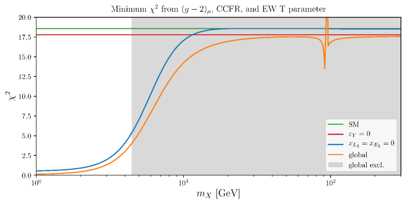
Figure 1: Minimum $\chi^{2}$ values in a model with a new $X_{\mu}$ vector boson coupling to second generation leptons with charges $x_{L_{2}}$ and $x_{E_{2}}$ and a kinetic mixing with the hypercharge gauge boson $\varepsilon_{Y}$ from a fit to experimental data taking into account $(g-2)_{\mu}$, CCFR, and the EW $T$ parameter (see the text for details). The orange curve is the global best fit $\chi^{2}$, the blue is the best fit in the absence of muon charges (dark photon), the red is the best fit for vanishing kinetic mixing, and the green line is the SM $\chi^{2}$. In the shaded grey region, $(g-2)_{\mu}$ cannot be explained by any values of $x_{L_{2}}$, $x_{E_{2}}$, and $\varepsilon_{Y}$ while at the same time satisfying the constraints from CCFR and the electroweak $T$ parameter.

We observe that at low $m_{X}$ masses, the best fit is similar to the solution where the $X_{\mu}$ couplings are exclusively generated by the kinetic mixing. However, as the $m_{X}$ mass increases there is a growing tension between a large value of $\varepsilon_{Y}$, which would minimize the size of the $X_{\mu}$ couplings to neutrinos and the effect of the trident constraints, and a small value as preferred by EWPT constraints. The net effect is that a combination of trident production and EWPT constraints limit the $X$ boson solutions to $(g-2)_{\mu}$ to be rather light:

$$m_{X}\lesssim 4\,\text{GeV}\qquad\text{(trident+$T$)}.$$ (31)

It is worth reiterating that the only assumptions entering this bound are that the $\mathrm{U}(1)_{X}$ model is renormalizable. Higher-dimensional operators could be added to the Lagrangian (6) to modify the bound; however, this goes beyond the minimality assumed in this paper.

4.2    Global constraints on anomaly-free vector-like $\mathrm{U}(1)_{X}$ models

Having set an overall upper bound on $m_{X}$, we perform a scan over all vector-like models in order to determine those that can account for the $(g-2)_{\mu}$ discrepancy and at the same time satisfy all the constraints discussed in Section 3. We assume that the sterile neutrinos are heavy enough so as not to affect the low energy phenomenology. The $\mathrm{U}(1)_{X}$ charges in the vector-like models then constitute a 3-parameter family of possible charge assignments, with the charges $x_{f}$ for each SM fermion given by

$$x_{f}=c_{B}B-c_{e}L_{e}-c_{\mu}L_{\mu}-c_{\tau}L_{\tau},\quad\text{where}\quad c_{B}=\frac{c_{e}+c_{\mu}+c_{\tau}}{3},$$ (32)

with $B$, $L_{e,\mu,\tau}$ the baryon and individual lepton numbers and $c_{e,\mu,\tau}$ continuous parameters. For the 419 vector-like models with $|x_{f}|\leq 10$, these take specific rational values that can be found in Ref. Greljo:2021npi . An overall factor can be absorbed into the gauge coupling $g_{X}$, which reduces the number of independent physical parameters to two. Since it is well-known that the $L_{\mu}-L_{\tau}$ model can explain $(g-2)_{\mu}$ while passing all constraints, we express the two-dimensional model space in Eq. (32) in a way that makes it apparent how closely a given model resembles the $L_{\mu}-L_{\tau}$ charge assignments,

$$x_{f}\propto\sin(\alpha)\big{(}L_{e}-L_{\mu})+\cos(\alpha)\big{(}B/3-L_{\mu}\big{)}+R\big{(}L_{\mu}-L_{\tau}\big{)}.$$ (33)

The polar angle $\alpha$ determines the ratio of baryon and electron charges, while the radial parameter $R$ gives the “closeness” to $L_{\mu}-L_{\tau}$, with $R\to\infty$ corresponding to the exact $L_{\mu}-L_{\tau}$ limit. Note that $L_{e}$ and $B$, with coefficients proportional to $\sin(\alpha)$ and $\cos(\alpha)$, respectively, enter the parameterization in a combination with $L_{\mu}$ in such a way that models given by Eq. (33) are anomaly-free for arbitrary values of $\alpha$ and $R$.

We use the parametrization (33) to systematically treat the experimental constraints on the vector-like models. Since only low $X$ mass explanations of $(g-2)_{\mu}$ are still possible, cf. Eq. (31), we can focus on the low-energy Lagrangian (1). For each vector-like model, the physics is determined by the $X$ mass $m_{X}$, the gauge coupling $g_{X}$, and the kinetic mixing parameter $\varepsilon$. To reduce the complexity of the analysis, we identify $m_{X}\simeq$200\text{\,}\mathrm{M}\mathrm{e}\mathrm{V}$$ as the mass with the best possibility of explaining $(g-2)_{\mu}$: for masses above the di-muon threshold the resonance searches at LHCb and Babar provide very strong constraints. All the remaining important bounds, in particular the bounds on NSI from neutrino oscillations, Borexino, NA64, and COHERENT, limit the $X$ mass from below, and thus taking $m_{X}$ close to the di-muon threshold minimizes their importance.

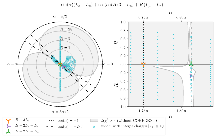
Figure 2: Bounds on vector-like gauge model solutions to $(g-2)_{\mu}$, parameterized by Eq. (33), at $m_{X}=$200\text{\,}\mathrm{M}\mathrm{e}\mathrm{V}$$. Inside the grey region, an explanation of $(g-2)_{\mu}$ is excluded by the combination of data from neutrino oscillations in matter, NA64, Borexino, BaBar 2014 (see text for details). The blue crosses correspond to models with integer charges $|x_{f}|\leq 10$. Linear and logarithmic scales are used for $R<1$ and $R>1$, respectively.

To narrow down the possible candidates for explaining $(g-2)_{\mu}$, we scan over $\alpha$ and $R$ in Eq. (33). For each point in the $(\alpha,R)$ model space, we construct a $\Delta\chi^{2}$ function that takes into account the bounds from $\Delta a_{\mu}$, Borexino, and NSI osc. and minimize it with respect to $(g_{X},\,\varepsilon)$ at $m_{X}=$200\text{\,}\mathrm{M}\mathrm{e}\mathrm{V}$$. As an additional constraint, we require $(g_{X},\,\varepsilon)$ to be in the range allowed by NA64 and BaBar2014 searches, as implemented in DarkCast. We deem a model to be excluded as a viable explanation of the $(g-2)_{\mu}$ anomaly, if the minimum $\Delta\chi^{2}$ value is above 4. This is to be compared with the SM value for $\Delta\chi^{2}$, which is $\Delta\chi^{2}\big{|}_{\rm SM}=18.3$), i.e., we discard models that are in tension with either $(g-2)_{\mu}$ or any individual constraint by more than 2$\sigma$. Further details on the construction of $\Delta\chi^{2}$ are given in Appendix B.

In the left panel of Fig. 2, we show the entire excluded region in the model space. For illustration, we mark all the models with integer charges $|x_{f}|\leq 10$ with small blue crosses and the three benchmark models $B-3L_{e}$, $B-2L_{e}-L_{\tau}$, and $B-2Le-L_{\mu}$ by orange, purple, and green tripods. As expected, for large values of the radial parameter, $R\gtrsim 50$, all the models are viable, irrespective of the value of $\alpha$. All such models closely resembles the $L_{\mu}-L_{\tau}$ model with only small deviations.

For smaller $R$ values the viability of the models is strongly $\alpha$ dependent, i.e., dependent on the baryon-to-electron charge ratio. For small values of $R$, the viable models are restricted to a narrow region around $\tan(\alpha)=-2/3$ (depicted as the black dashed line in Fig. 2 left) so that the $\mathrm{U}(1)_{X}$ electron charge is roughly $-2$ times the baryon charge. For such charge assignments, normal planetary matter, which has on average about as many protons as neutrons, is almost neutral under $\mathrm{U}(1)_{X}$. As discussed in Section 3.3, this results in the reduced relevance of neutrino oscillation constraints. By contrast, the $\mathrm{U}(1)_{X}$ models in which normal matter carries a considerable $\mathrm{U}(1)_{X}$ charge are ruled out as an explanation of $(g-2)_{\mu}$ precisely because of the excessive contributions to the NSI. There are only two ways for a model to both explain $(g-2)_{\mu}$ and predict the atoms of the most common elements to be essentially $\mathrm{U}(1)_{X}$-neutral. Either $\tan(\alpha)\approx-2/3$ so the electron and nucleon charges approximately cancel, or $R\gg 1$ so the electron and nucleon charges are small compared to the muon charge. The only model in which all atoms are exactly $\mathrm{U}(1)_{X}$-neutral is the $L_{\mu}-L_{\tau}$ model, i.e., $R\to\infty$. For models that differ considerably from $L_{\mu}-L_{\tau}$, i.e., for  $R\ll 1$, the cancellation of $\mathrm{U}(1)_{X}$ charges in normal matter is the only way to avoid the stringent NSI bounds.

In the right panel of Fig. 2, we show the region around $\tan(\alpha)\approx-2/3$ for $R<1$. Again, we mark the models with integer charges $|x_{f}|\leq 10$ with small blue crosses and the three sample models $B-3L_{e}$, $B-2Le-L_{\tau}$, and $B-2Le-L_{\mu}$ with orange, purple, and green tripods, respectively. In the lower half of the plot $\alpha$ is shifted by $\pi$ compared to the upper half of the plot, and $R$ is always positive. We observe that for small values of $R$, the only models that can pass the neutrino oscillation bounds either lie in a very narrow region close to $\tan(\alpha)=-2/3$, where nucleon and electron $\mathrm{U}(1)_{X}$ charges cancel inside atoms, or at around $R\approx 0.1$ in the region $-1\lesssim\tan(\alpha)\lesssim-2/3$.

Charges				Best-fit values for $m_{X}=200$ MeV					Fig.
$c_{B}$	$c_{e}$	$c_{\mu}$	$c_{\tau}$	$\varepsilon\,{e}/{g_{X}}$		$g_{X}$		$\Delta\chi^{2}$	panel
$0$	$0$	$1$	$-1$	$0.01$		$1.44\times 10^{-3}$		$0.41$	Fig. 3
$3$	$-7$	$-1$	$-1$	$-6.97$		$2.17\times 10^{-4}$		$2.00$	Fig. 5 f)
$3$	$-6$	$7$	$-10$	$-6.26$		$1.02\times 10^{-4}$		$2.60$	Fig. 5 e)
$3$	$-6$	$6$	$-9$	$-6.21$		$9.90\times 10^{-4}$		$2.84$	Fig. 5 d)
$3$	$-6$	$5$	$-8$	$-6.16$		$1.19\times 10^{-4}$		$3.13$	Fig. 5 c)
$3$	$-6$	$4$	$-7$	$-6.11$		$1.31\times 10^{-4}$		$3.47$	Fig. 5 b)
$3$	$-6$	$3$	$-6$	$-6.08$		$1.30\times 10^{-3}$		$3.90$	Fig. 5 a)

Table 1: The $\mathrm{U}(1)_{X}$ charges parametrized by $c_{B,e,\mu,\tau}$ in (32) (first four columns), and the best-fit values of the mixing parameter (fifth column) and gauge coupling (sixth column), as well as the $\chi^{2}$ value at the minimum taking $m_{X}=200$ MeV, for vector-like $\mathrm{U}(1)_{X}$ models that can explain the measurement of $(g-2)_{\mu}$ within $2\sigma$ and pass the bounds from NSI osc., COHERENT, Borexino, NA64, and BaBar.

The constraints from neutrino oscillations on NSI already exclude most of the parameter space for $R\lesssim 10$. Another potentially relevant constraint in this region of model space is due to coherent elastic neutrino-nucleus scattering as measured by the COHERENT experiment. We impose this bound on all the models with integer charges $|x_{f}|\leq 10$ that are not already excluded by the neutrino oscillation data. (Since deriving the COHERENT bound is computationally expensive this constraints was not include in Fig. 2.) All the models that are not yet excluded before applying the COHERENT constraint appear in the right panel of Fig. 2 as small blue crosses on white background, apart from the $L_{\mu}-L_{\tau}$ model, which is not shown, since it corresponds to $R\to\infty$ limit. For all these models, we add the contribution from COHERENT to the previous $\Delta\chi^{2}$ function and minimize the newly obtained $\Delta\chi^{2}$ function at $m_{X}=$200\text{\,}\mathrm{M}\mathrm{e}\mathrm{V}$$ with respect to $(g_{X},\,\varepsilon)$. The charges and best-fit values of the models with $\Delta\chi^{2}<4$ are shown in Table 1. This table shows models belonging to three distinct classes, which we discuss separately next.

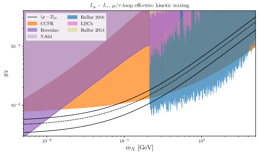
Figure 3: Parameter space of the $L_{\mu}-L_{\tau}$ model with the parameter space that explains the central value of $\Delta a_{\mu}$ denoted with dashed black line (the $2\sigma$ band by solid black lines). The exclusions by different measurements are color coded as given in the legend.

The $L_{\mu}-L_{\tau}$ model

The $L_{\mu}-L_{\tau}$ model has the lowest $\Delta\chi^{2}$ value. It is able to explain $(g-2)_{\mu}$ comfortably without causing tensions with other experimental constraints. The best-fit point is found for vanishing kinetic mixing $\varepsilon$, however even for kinetic mixing values that one would typically obtain if this were generated at one loop, $\varepsilon\sim g_{X}\,e/(16\pi^{2})$, the $L_{\mu}-L_{\tau}$ model can still explain $(g-2)_{\mu}$ without being excluded by other constraints. In Fig. 3 we show an example where the kinetic mixing is assumed to be induced by the muon and tau running in the loop.

The class $3B-6L_{e}-3L_{\tau}+N(L_{\mu}-L_{\tau})$ with $N\in\{3,4,5,6,7\}$

These models satisfy $\tan(\alpha)=-2/3$, i.e., they lie on the dashed vertical line in Fig. 2 and are all within the narrow region of model space where the $\mathrm{U}(1)_{X}$ charges of electrons and nucleons in atoms approximately cancel. In Fig. 2, only the models with $N<-2$ were excluded. The addition of the COHERENT constraint now leads to the exclusion of all models with $N<3$. As shown in Table 1, larger values of $N$ generically correspond to lower $\Delta\chi^{2}$ values, that is, they can satisfy the constraints more easily. This is visualized in the left panel of Fig. 4, where we show the $\Delta\chi^{2}$ values for $N\geq 0$ with the grey shaded region corresponding to $\Delta\chi^{2}>4$. The reason for the decrease in $\Delta\chi^{2}$ as $N$ increases is that the muon charge increases as well and thus a smaller gauge coupling is requires to explain $(g-2)_{\mu}$. This can be seen in the sixth column of Table 1 and in the right panel of Fig. 4. Since an increase in $N$ does not affect electron and baryon charges, the smaller values of the gauge coupling lead to weaker constraints from NSI. Ultimately, the models become more similar to the $L_{\mu}-L_{\tau}$ model as $N$ increases.

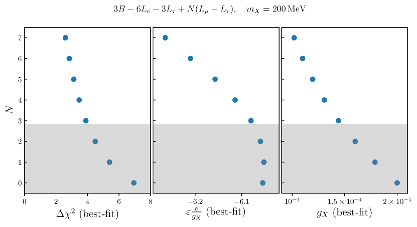
Figure 4: The comparison of minimal $\Delta\chi^{2}$ values (left panel), as well as best-fit values for the kinetic mixing parameter (middle) and the gauge coupling (right) for the vector-like $\mathrm{U}(1)_{X}$ models with the SM fermion charges parametrized as $x_{f}=3B-6L_{e}-3L_{\tau}+N(L_{\mu}-L_{\tau})$, with $N\in\{0,1,2,3,4,5,6,7\}$. The $\Delta\chi^{2}$ function takes into account the measurement of $(g-2)_{\mu}$ and the bounds from NSI osc., COHERENT, Borexino, NA64, and BaBar while the $X$ mass was set to 200 MeV. The grey shaded region corresponds to $\Delta\chi^{2}>4$. The five models with $\Delta\chi^{2}<4$ are also listed in Table 1.

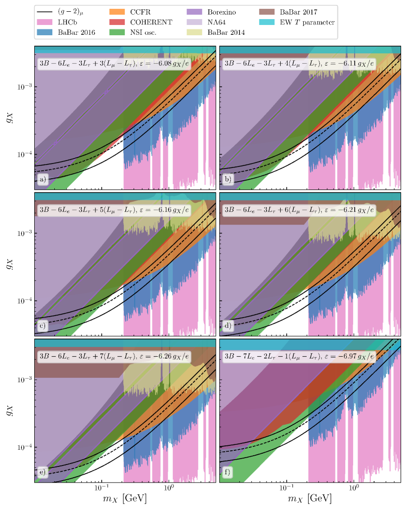
Figure 5: Parameter space of viable vectorlike $\mathrm{U}(1)_{X}$ models that can explain $(g-2)_{\mu}$ (the parameter space for $L_{\mu}-L_{\tau}$ is shown in Fig. 3). The central value of $\Delta a_{\mu}$ is indicated by a dashed black line (the $2\sigma$ band by solid black lines). The exclusions by different measurements are color coded as given in the legend.

At the best-fit point, not only the $\Delta\chi^{2}$ value and the gauge coupling $g_{X}$ but also the kinetic mixing $\varepsilon$ is correlated with $N$, which can be understood as follows: The COHERENT bound is due to a measurement of the coherent elastic neutrino-nucleus scattering in cesium iodide (CsI). Accordingly, the COHERENT bound becomes less constraining if the $\mathrm{U}(1)_{X}$ charges of protons and neutrons in CsI approximately cancel. Cesium and iodine have neutron-to-proton ratios $78/55$ and $74/53$, respectively, such that the average neutron-to-proton ratio in CsI is $1.4$ to a very good approximation. In the $3B-6L_{e}-3L_{\tau}+N(L_{\mu}-L_{\tau})$ class of models, the effective $\mathrm{U}(1)_{X}$ charge of neutron and proton (taking into account the kinetic mixing $\varepsilon$) is $3$ and $3+\varepsilon\,{e}/{g_{X}}$, respectively. CsI therefore becomes approximately $\mathrm{U}(1)_{X}$-neutral for

$$3+\varepsilon\frac{e}{g_{X}}\approx-(1.4\times 3)\qquad\implies\qquad\varepsilon\frac{e}{g_{X}}\approx-7.2\,.$$ (34)

The Borexino bound, on the other hand, is due to a measurement of elastic neutrino-electron scattering and vanishes if the effective $\mathrm{U}(1)_{X}$ charge of the electron is zero, i.e., when

$$-6-\varepsilon\frac{e}{g_{X}}=0\qquad\implies\qquad\varepsilon\frac{e}{g_{X}}=-6\,.$$ (35)

For small $N$, the relatively large gauge coupling needed to explain $(g-2)_{\mu}$ makes the Borexino bound very sensitive to deviations from Eq. (35). As $N$ increases and the gauge coupling decreases, larger deviations from Eq. (35) are allowed by Borexino and the best fit value of $\varepsilon\,{e}/{g_{X}}$ moves closer to Eq. (34) in order to better satisfy the COHERENT bound. This also means that the COHERENT bound is considerably more constraining at the best fit point for smaller $N$, which in turn leads to a larger $\Delta\chi^{2}$ value.

The bounds on $3B-6L_{e}-3L_{\tau}+N(L_{\mu}-L_{\tau})$ with $N\in\{3,4,5,6,7\}$ are shown in Fig. 5 in panels a) through e), in the plane of the $X$ mass $m_{X}$ and the gauge coupling $g_{X}$, while for each plot the kinetic mixing $\varepsilon$ is set to its best-fit value shown in Table 1. In these plots, we can observe the interplay of Borexino and COHERENT constraints described above. For small $N$, e.g., for $N=3$ shown in panel a), $g_{X}$ has to be relatively large in order to explain $(g-2)_{\mu}$. Consequently, the Borexino bound (shown in dark purple) requires $\varepsilon$ to be very close to Eq. (35). This in turn leads to a relatively strong COHERENT bound (shown in red), which then excludes part of the parameter region preferred by $(g-2)_{\mu}$ in the $m_{X}$ mass range between $100\text{\,}\mathrm{M}\mathrm{e}\mathrm{V}$ and $200\text{\,}\mathrm{M}\mathrm{e}\mathrm{V}$. Comparing this to the models with increasing $N$ in panels b) through e), one observes that the size of $g_{X}$ preferred by $(g-2)_{\mu}$ decreases due to the increasing muon charge, the Borexino bound allows for smaller $\varepsilon$, and the COHERENT bound becomes less and less important until it becomes weaker than the bound from the neutrino oscillations for $N=7$, cf. panel e).

The plots in Fig. 5 also demonstrate that for $m_{X}$ above the dimuon threshold, resonance searches, in particular from BaBar and LHCb, prevent an explanation of $(g-2)_{\mu}$, whereas for lower values of $m_{X}$, neutrino oscillation data provides the strongest bound. This justifies the choice of $m_{X}=$200\text{\,}\mathrm{M}\mathrm{e}\mathrm{V}$$ used in Figs. 2 and 4 and Table 1.

It is interesting that the CCFR bound from neutrino trident production (shown in orange) becomes less constraining for smaller values of $N$ and even completely disappears for $N=0$. The reason is that the effective $\mathrm{U}(1)_{X}$ couplings of the charged muon and muon neutrino are $N-\varepsilon\,{e}/{g_{X}}$ and $N$, respectively. For sizable $\varepsilon$ and decreasing $N$, the region in parameters space where $(g-2)_{\mu}$ can be explained is, therefore, less and less excluded by the CCFR bound. In the large $N$ limit, on the other hand, the model is closer and closer to the $L_{\mu}-L_{\tau}$ model and the CCFR constraint becomes increasingly important.

The class $3B-7L_{e}-2L_{\tau}+N(L_{\mu}-L_{\tau})$ with $N=-1$

These models satisfy $\tan(\alpha)=-7/9$ so that the cancellation of $\mathrm{U}(1)_{X}$ charges inside atoms is less efficient than in the models with $\tan(\alpha)=-2/3$. Nevertheless, there is a window roughly around $N=-1$ where the bound from neutrino oscillations is relatively weak and an explanation of $(g-2)_{\mu}$ is possible (cf. right panel of Fig. 2). The virtue of this class of models is that both the Borexino and the COHERENT bounds can be comfortably satisfied. This is apparent from the constraints displayed in Fig. 5, panel f), which show that for $m_{X}$ below the dimuon threshold the neutrino oscillations provide the most relevant bound in the $(g-2)_{\mu}$ band, whereas COHERENT and Borexino are far less important. While the COHERENT bound vanishes for $\varepsilon\,{e}/{g_{X}}\approx-7.2$, as in Eq. (34), the effective $\mathrm{U}(1)_{X}$ charge of the electron in the present class of models is $-7-\varepsilon\,{e}/{g_{X}}$ such that the Borexino bound disappears for $\varepsilon\,{e}/{g_{X}}=-7$. Consequently, values of $\varepsilon\,{e}/{g_{X}}\approx-7$ lead to very weak bounds for both Borexino and COHERENT. The best fit values for $\varepsilon\,{e}/{g_{X}}$ are indeed found to be very close to $-7$ by the global scan (see Table 1). The only model in the class $3B-7L_{e}-2L_{\tau}+N(L_{\mu}-L_{\tau})$ that enters the list of viable models in Table 1 is the one with $N=-1$, but it actually reaches the second lowest $\Delta\chi^{2}$ of all the models in this list. This model is also notable for particularly weak bounds from neutrino trident production.

5    Chiral models

There are 21 chiral charge assignments in the charge range $[-10,10]$ (not counting permutations) in which lepton masses cannot be fully realised at the renormalizable level Greljo:2021xmg . Upon careful inspection of the charge assignments in the entire class of the chiral $\mathrm{U}(1)_{X}$ models, we focus on one of the best performing models, the model $\tilde{L}_{\mu-\tau}$. Quite generally, for these types of models the constraints in the parameter region relevant for $(g-2)_{\mu}$ will be minimized, if the $\mathrm{U}(1)_{X}$ charges of the quarks vanish, and the electron coupling is purely axial, in order to avoid the NSI bounds, while the vector-like muon charge is as large as possible. The $\tilde{L}_{\mu-\tau}$ model satisfies all of the above requirements. Even so, the $\tilde{L}_{\mu-\tau}$ model is excluded as the explanation of the $(g-2)_{\mu}$ anomaly by a set of complementary constraints, as we show below, and we expect the same to be true for the other chiral models.

In the $\tilde{L}_{\mu-\tau}$ model, the $\mathrm{U}(1)_{X}$ charges of the fermions are given by Greljo:2021npi

$$(x_{L_{1}},\,x_{L_{2}},\,x_{L_{3}}) =(-1,7,-6),$$ (36a)

$$(x_{E_{1}},\,x_{E_{2}},\,x_{E_{3}}) =(1,6,-7),$$ (36b)

$$(x_{N_{1}},\,x_{N_{2}},\,x_{N_{3}}) =(-7,-2,9),$$ (36c)

$$x_{Q_{i},D_{i},U_{i}} =0,$$ (36d)

where the first line is for the left-handed leptons, the second and the third lines are for the right-handed charged leptons and neutrinos, respectively, while the quarks do not carry a $\mathrm{U}(1)_{X}$ charge.

Due to the $\mathrm{U}(1)_{X}$ charge assignment, the charged lepton Yukawas are forbidden at the renormalizable level and only arise once the $\mathrm{U}(1)_{X}$ gauge symmetry is spontaneously broken. For concreteness let us consider the minimal possibility—that it is due to a SM-singlet scalar $\phi$ with $\mathrm{U}(1)_{X}$ charge $x_{\phi}=1$ that develops a VEV $\langle\phi\rangle\neq 0$. The diagonal entries of the charged lepton Yukawa matrix are populated by the dimension-5 operators $\bar{L}_{i}H\phi^{\dagger}E_{i}$ for muons and taus, $i=2,3$, and by the dimension-6 operator $\bar{L}_{1}H\phi^{2}E_{1}$ for the electrons. This is consistent with the smallness of the charged lepton masses and with the hierarchy between electron and muon and tau Yukawas. Such higher-dimension operators can be generated, for instance, by integrating out a set of heavy vector-like leptons at tree level with masses $M\gg\langle\phi\rangle$ well above the EW scale. The muon and tau Yukawas are then suppressed by $\langle\phi\rangle/M$ and the electron Yukawa by $(\langle\phi\rangle/M)^{2}$.

The off-diagonal terms in the Yukawa matrix are predicted to be zero up to corrections from operators of dimension 10 or higher, assuming that the necessary fields required to mediate such off-diagonal operators are even present in the UV theory. The suppressed mixing provides the needed protection against cLFV constraints. A phenomenologically viable realization of the neutrino masses and mixings, on the other hand, requires additional scalars. Thanks to the smallness of the neutrino masses, this can be done consistently without introducing sizeable cLFV.

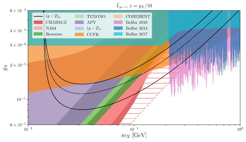
Figure 6: Parameter space for the light $X$ solution to the $(g-2)_{\mu}$ anomaly in the $\tilde{L}_{\mu-\tau}$ model. The shaded regions are excluded by various experiments, while the region between the black lines is preferred by $(g-2)_{\mu}$ at $2\sigma$. See Section 5 for details.

The $2\sigma$ band in parameter space of $\tilde{L}_{\mu-\tau}$ that explains $(g-2)_{\mu}$ is denoted with solid-black lines in Fig. 6 (dashed black line denotes the central value), while the colored regions are excluded. The neutrino trident CCFR bound (orange) limits the $\tilde{L}_{\mu-\tau}$ solution of $(g-2)_{\mu}$ to $m_{X}\lesssim$400\text{\,}\mathrm{M}\mathrm{e}\mathrm{V}$$. In Fig. 6 the kinetic mixing parameter was set to $\varepsilon=g_{X}/10$, comparable to the IR contribution from muon and tau running in the loop, cf. Eq. (40) below. For larger values of $\varepsilon$, the atomic parity violation constraints (dark purple) become more stringent (see Section 5.1). The upper limit on $\varepsilon$ from atomic parity violation makes the CCFR bound very robust, i.e., the trident can not be removed by choosing $\varepsilon$ as in the vector category.

The Borexino bound on neutrino–electron scattering (dark green) limits the $\tilde{L}_{\mu-\tau}$ solution of $(g-2)_{\mu}$ to the $X$ masses above $m_{X}\gtrsim$60\text{\,}\mathrm{M}\mathrm{e}\mathrm{V}$$. The NSI oscillation bounds, on the other hand, are not relevant for the $\tilde{L}_{\mu-\tau}$ model, since in $\tilde{L}_{\mu-\tau}$ the couplings of $X_{\mu}$ to electrons are purely axial and, thus, induce only suppressed, spin-dependent effects. Furthermore, in $\tilde{L}_{\mu-\tau}$ the $X$ boson does not couple to quarks. These two features of $\tilde{L}_{\mu-\tau}$ couplings mean that the NSI oscillation bounds are completely avoided in this model.

The constraints from the resonant searches are obtained using the DarkCast code which by default supports only vector couplings. We approximate the $\tilde{L}_{\mu-\tau}$ bounds with those for a vector model with charges $x_{L_{1},L_{2},L_{3}}=(1,\,\frac{13}{2},\,-\frac{13}{2})$. For processes where the mass can be neglected, such as NA64, there is no difference between the axial and the vectorial couplings. Also for the BaBar search, the above vector model reinterpretation still approximates rather well the actual bounds Kahn:2016vjr ; axial:DarkCast . Below the di-muon threshold, the dominate decay channel of $X$ is to invisible final states, while above the di-muon threshold there is a sizeable branching ratio for $X\to\mu^{+}\mu^{-}$. The $e^{+}e^{-}$ decay mode is suppressed because of the charge hierarchy and gives a sub-leading constraint. In all cases, the $X$ decays are prompt in the targeted parameter space. The resonance searches rule out the $\tilde{L}_{\mu-\tau}$ solution to $(g-2)_{\mu}$ for $m_{X}>2m_{\mu}$ (BaBar) and for $m_{X}\lesssim 100$ MeV (NA64).

Since $\tilde{L}_{\mu-\tau}$ has chiral couplings, there are also observables that are only important for such cases of combined vector and axial vector couplings to SM fermions, which we discuss next.

5.1    Atomic parity violation

Parity-violating atomic transitions can determine whether $X$ couples axially to electrons. For typical momentum transfers in atomic interactions $q^{2}\ll m_{X}^{2}$ (for the mass range considered here) and the tree-level exchange of $X$ leads to an effective interaction,

$$\mathcal{L}_{\mathrm{eff}}\supset\dfrac{\varepsilon\,e\,g_{X}}{m_{X}^{2}}(\bar{e}\gamma_{\mu}\gamma_{5}e)(\tfrac{2}{3}\bar{u}\gamma^{\mu}u-\tfrac{1}{3}\bar{d}\gamma^{\mu}d),$$ (37)

where the couplings to quarks are due to kinetic mixing. The effect of $X$ on the Hamiltonian of atomic systems is, thus, modeled with a parity-violating point-like interaction between the electric charge of the nucleus and electrons and mimics the parity-violating interaction between the nucleus and electrons mediated by the exchange of the SM $Z$ boson. Hence, the new muonic force can be seen as a modification of the weak charge of the nucleus Arcadi:2019uif ,

$$\Delta Q_{\mathrm{weak}}=Z\,\varepsilon\,e\,g_{X}\dfrac{2\sqrt{2}}{G_{F}m_{X}^{2}},$$ (38)

where $Z$ is the atomic number.

The parity-violating transition has been measured to percent-level precision in $\phantom{}{}_{55}^{133}\mathrm{Cs}$ Porsev:2009pr , with the latest analysis finding $Q^{\mathrm{exp}}_{\mathrm{weak}}-Q^{{\scriptscriptstyle\mathrm{SM}}}_{\mathrm{weak}}=$0.65\pm 0.43$$ Dzuba:2012kx . We can use this to place the $95\%$ CL bound on the atomic parity violating (APV) couplings of the $X$ boson,

$$g_{X}<\dfrac{m_{X}}{$1\text{\,}\mathrm{G}\mathrm{e}\mathrm{V}$}\left(\dfrac{|\varepsilon|e}{g_{X}}\right)^{\!\!\vbox{\hbox{\scalebox{0.6}[1.0]{$-$}}}1/2}\begin{dcases}$3.4\text{\times}{10}^{-4}$&\mathrm{for}\;\varepsilon>0\\ $1.3\text{\times}{10}^{-4}$&\mathrm{for}\;\varepsilon<0\end{dcases}.$$ (39)

With no particular UV theory in mind, $\varepsilon$ is treated as a free parameter, and the APV bound can be evaded by sufficiently reducing the value of $\varepsilon$. Nevertheless, the running of $\varepsilon$ can be used to set an approximate lower bound on $|\varepsilon|$ in the absence of tuning. Assuming no other BSM particles below the scale of electroweak symmetry-breaking and working in the limit $\varepsilon\ll g_{X}$, the 1-loop running of $\varepsilon$ receives its dominant contribution from renormalization group running between the muon and tau mass Greljo:2021npi , resulting in

$$\varepsilon(m_{\mu})-\varepsilon(m_{\tau})\simeq\dfrac{13e\,g_{X}}{12\pi^{2}}\ln\dfrac{m_{\tau}}{m_{\mu}}=0.31e\,g_{X}.$$ (40)

For processes with small momentum transfers, we therefore expect $\varepsilon\gtrsim g_{X}/10$. At high scales, where other states, such as the putative $S_{3}$ muoquark, are dynamical, these can also contribute to the running of $\varepsilon$, which should be taken into account in any UV completion of the model.

The presence of a rather stringent APV bound, Eq. (39), has important phenomenological implications. It excludes the possibility of the $X$ coupling to muons being dominated by the kinetic mixing, which could otherwise decorrelate the couplings to muons and muon neutrinos, cf. Section 3.2. This is not possible for $\tilde{L}_{\mu-\tau}$ . Since in this model the interactions of $X_{\mu}$ with nucleus are induced by the kinetic mixing, the COHERENT bound in Fig. 6 (light orange) can be directly compared with the one from APV (dark purple), the latter being stronger.

5.2    Electron anomalous magnetic moment

The second observable for which the $\tilde{L}_{\mu-\tau}$ model is qualitatively different from a vector-like model such as $L_{\mu}-L_{\tau}$ is the electron anomalous magnetic moment, $(g-2)_{e}$. In $L_{\mu}-L_{\tau}$ the $X$ coupling to electrons is exclusively due to a (presumed) small kinetic mixing with the photon, resulting in a similarly minute modification of $(g-2)_{e}$. In the $\tilde{L}_{\mu-\tau}$ model, on the other hand, the electron carries a nonzero $\mathrm{U}(1)_{X}$ charge and receives a much larger contributions to $(g-2)_{e}$ (the contribution is also numerically larger because of the coupling to electrons is axial, cf. Eq. (5)).

The $(g-2)_{e}$ has been calculated to high precision in the SM Aoyama:2014sxa but crucially depends on the exact value of the fine-structure constant. Recently, $\alpha$ has been measured precisely in two experiments involving cesium Parker:2018vye and rubidium Morel:2020dww atoms, respectively; however, the measurements are internally inconsistent at the level of $5.4\sigma$. With these inputs, the deviation of the measured $(g-2)_{e}$ Hanneke:2008tm from the SM theory prediction is found to be $a_{e}^{\mathrm{exp}}-a_{e}^{{\scriptscriptstyle\mathrm{SM}},\mathrm{Cs}}=(-8.8\pm 3.6)\cdot 10^{-13}$ and $a_{e}^{\mathrm{exp}}-a_{e}^{{\scriptscriptstyle\mathrm{SM}},\mathrm{Rb}}=(4.8\pm 3.0)\cdot 10^{-13}$, with errors dominated by the experimental measurement of $(g-2)_{e}$.

In the $\tilde{L}_{\mu-\tau}$ model, the axial coupling of $X$ to the electron gives a negative correction to $(g-2)_{e}$ (see, e.g., Refs. Jackiw:1972jz ; Jegerlehner:2009ry ). Working in the limit $m_{X}\gg m_{e}$, this translates into 95% CL bounds

$$g_{X}<$9.5\text{\times}{10}^{-3}$\dfrac{m_{X}}{$1\text{\,}\mathrm{G}\mathrm{e}\mathrm{V}$}(-\Delta a_{e})=\begin{dcases}$1.2\text{\times}{10}^{-2}$&\text{[Cs]},\\ $3.3\text{\times}{10}^{-3}$&\text{[Rb]}.\end{dcases}$$ (41)

A stronger bound is obtained using $\alpha$ from the rubidium measurement, which prefers a positive contribution to $(g-2)_{e}$. However, even this constraint is still weaker than the Borexino bound as shown in Fig. 6.

5.3    Neutrino-electron scattering

The reactor experiments TEXONO TEXONO:2009knm and GEMMA Beda:2009kx measured the neutrino scattering on electrons and set competitive constraints on the $X_{\mu}$ couplings. The relevant bound shown in Fig. 6 is extracted using the $\bar{\nu}_{e}e^{-}\to\bar{\nu}_{e}e^{-}$ electron recoil energy spectrum from Fig. 16(b) of the TEXONO analysis paper, Ref TEXONO:2009knm , closely following the procedure described in Lindner:2018kjo . For $\tilde{L}_{\mu-\tau}$, we find the $95\%$ CL bounds

$$g_{X}<1.7\times 10^{-4}\frac{m_{X}}{100\leavevmode\nobreak\ \rm{MeV}}\leavevmode\nobreak\ ,$$ (42)

and $2.8\times 10^{-4}<g_{X}\times 100\leavevmode\nobreak\ {\rm MeV}/m_{X}<3.5\times 10^{-4}$, where the NP amplitude is roughly twice the negative SM amplitude. The electron recoil energy is $\lesssim 8$ MeV, thus, the above EFT limit is valid for the $m_{X}$ range considered in Fig. 6. This bound is only slightly worse than the Borexino bound.

The high-energy beam experiment CHARM-II at CERN measured elastic $\nu_{\mu}e^{-}$ and $\bar{\nu}_{\mu}e^{-}$ scattering CHARM-II:1993phx ; CHARM-II:1994dzw . The target calorimeter was exposed to the horn-focused wide band neutrino beam from the Super Proton Synchrotron with the mean muon neutrino (antineutrino) energy of $E_{\nu}=23.7\pm 0.3$ GeV ($E_{\nu}=19.1\pm 0.2$ GeV). The signature of this process is a forward-scattered electron producing an electromagnetic shower measured by the calorimeter. The variable $y$ is defined as the ratio of the electron recoil energy over the incident neutrino energy. Neglecting the electron mass, the differential cross section is given by

$$\frac{d\sigma}{dy}(\nu_{\mu}e,\bar{\nu}_{\mu}e)=\frac{2G_{F}^{2}E_{\nu}m_{e}}{\pi}\left(g_{\mathrm{L},\mathrm{R}}^{2}+g_{\mathrm{R},\mathrm{L}}^{2}(1-y)^{2}\right)\leavevmode\nobreak\ ,$$ (43)

where

$$g_{\mathrm{L}} =s_{w}^{2}-\frac{1}{2}+\frac{g_{X}^{2}x_{L_{2}}x_{L_{1}}}{2\sqrt{2}G_{F}(2E_{\nu}m_{e}y+m_{X}^{2})},$$ (44)

$$g_{\mathrm{R}} =s_{w}^{2}+\frac{g_{X}^{2}x_{L_{2}}x_{E_{1}}}{2\sqrt{2}G_{F}(2E_{\nu}m_{e}y+m_{X}^{2})},$$ (45)

where the $X$ charges of the $\tilde{L}_{\mu-\tau}$ model are given in Eq. (36).

The unfolded differential distributions in $y$ for $\nu_{\mu}e$ and $\bar{\nu}_{\mu}e$ scattering were reported in Fig. 1 of Ref. CHARM-II:1993phx , albeit in arbitrary units. This information was then used in Ref. CHARM-II:1993phx to determine the SM weak mixing angle by fitting to the shape of the distributions, while requiring no knowledge of the overall normalization. Similarly, in $\tilde{L}_{\mu-\tau}$ we are able to set an upper bound on $g_{X}$ for given $m_{X}$ by profiling over two arbitrary nuisance parameters describing the absolute normalisations. The excluded region is shown with red color in Fig. 6. This represents the most stringent limit on the model for $m_{X}\lesssim 100$ MeV.

The shape analysis is unfortunately ineffective for larger masses where the information on the overall rate is needed. Although the SM prediction was overlaid in Fig. 1 of Ref. CHARM-II:1993phx , the uncertainty on the prediction was not reported. The expected SM cross section depends on the number of factors subject to systematic uncertainties such as the neutrino flux determination. Conservatively assuming the error on the normalisation of the SM prediction to be $30\%$, i.e., constraining the two nuisance parameters in the fit to be $1.0\pm 0.3$, we find the exclusion shown with the red-hatched region in Fig. 6, covering the remaining viable mass window for $(g-2)_{\mu}$. While the estimate of a 30% error on overall normalization seems plausible to us, if not even conservative (it is an order of magnitude larger than the relative error in the determination of $g_{A}^{\nu e}$ CHARM-II:1994dzw ), it is not sufficient to claim a definitive exclusion of the $\tilde{L}_{\mu-\tau}$ model. A proper recast of the CHARM-II bound using the detector level events shown in Fig. 1 of Ref. CHARM-II:1994dzw while accounting correctly for the systematic effects could possibly achieve this, but it is beyond the scope of this work.

6    Possible connections to $B$-anomalies

We continue by commenting on the possibility that a single vector mediator is behind a simultaneous solution of $(g-2)_{\mu}$ and $B$ anomalies. As shown in Section 4.1, there is a generic upper bound on the vector mass from neutrino trident production and $T$ parameter, $m_{X}\lesssim 4$ GeV. In this situation, $B\to K\nu\bar{\nu}$ provides an important bound since it receives contributions from on-shell $B\to KX$ decay. Generically, $X$ decays invisibly with a sizeable branching ratio. As shown in Ref. Greljo:2021npi , this puts an upper limit on the effective $g_{bs}$ coupling for a given $m_{X}$. Since the deviation in $R_{K}$ is proportional to the product of $g_{bs}$ and the effective $g_{\mu\mu}$ coupling, the two together imply a lower bound on $g_{\mu\mu}$ for given $m_{X}$, restricting the viable parameter space to be in the orange region in Figure 1 of Ref. Greljo:2021npi . The range predicted for the effective $g_{\mu\mu}$ coupling from the $(g-2)_{\mu}$ anomaly, on the other hand, does not overlap with the orange band in Figure 1 of Ref. Greljo:2021npi , apart from the small region around $m_{X}\sim 2.5$ GeV and $q_{A}/q_{V}\simeq-0.4$ (see also, e.g., Ref. Crivellin:2022obd ). This possibility is ruled out by the constraints on the trident production in the case of a small kinetic mixing. When the requirement of vanishingly small kinetic mixing is relaxed, this conclusion no longer applies in full generality, since the kinetic mixing can be used to remove the trident constraint. One then needs to invoke constraints from resonance searches to rule out explicit models.

A better way to solve the $B$ anomalies in this framework is to extend the field content by a heavy scalar, a TeV-scale muoquark $S_{3}$ in the $(\overline{\mathbf{3}},\,\mathbf{3},\,1/3)_{x_{S_{3}}}$ representation of the SM gauge group $\mathrm{SU}(3)_{c}\times\mathrm{SU}(2)_{\mathrm{L}}\times\mathrm{U}(1)_{Y}$ and with the $\mathrm{U}(1)_{X}$ charge $x_{S_{3}}=-x_{L_{2}}-x_{q}$ for $x_{L_{2}}\neq x_{L_{1},L_{3}}$. These charge assignments allow a Yukawa coupling ($\bar{q}^{c}\ell S_{3}$) of the muoquark to $\mu$ but not to $e$ and $\tau$. Furthermore, for $x_{L_{2}}\neq-3x_{q}$, the dimension-4 diquark operators $qqS_{3}^{\dagger}$ are forbidden and proton decay is suppressed. In other words, a non-universal $\mathrm{U}(1)_{X}$ enhances the properties of a TeV-scale leptoquark by keeping the accidental symmetries of the SM while still addressing $B$-anomalies Greljo:2021xmg ; Davighi:2020qqa ; Hambye:2017qix ; Davighi:2022qgb ; Heeck:2022znj . Out of 276 quark-flavor universal $\mathrm{U}(1)_{X}$ charge assignments, 273 allow for the above conditions for inclusion of a muoquark Greljo:2021npi . The three models which fail are: the dark photon model, which has $x_{f}=0$ for all fermions, and the $\mathrm{U}(1)_{B-L}$ and $\mathrm{U}(1)_{N_{i}-N_{j}}$ models. The $b\to s\mu^{+}\mu^{-}$ anomaly is resolved by a tree-level exchange of a TeV-scale $S_{3}$ muoquark. This exchange leads to an additional $V-A$ contribution to the $b\to s\mu^{+}\mu^{-}$ transitions, as required by data; see, e.g., Refs. Greljo:2021xmg ; Davighi:2020qqa ; Hiller:2014yaa ; Dorsner:2016wpm ; Buttazzo:2017ixm ; Crivellin:2017zlb ; Hiller:2017bzc ; Gherardi:2020qhc ; Angelescu:2021lln ; Marzocca:2018wcf ; Dorsner:2017ufx ; Babu:2020hun .

7    Conclusions

A new massive spin-1 boson $X_{\mu}$ coupling vectorially to muons, $\mathcal{L}\supset g_{X}q_{V}\bar{\mu}\gamma^{\mu}\mu\,X_{\mu}$, can give a one-loop contribution of the right size to explain the $4.2\sigma$ discrepancy in $(g-2)_{\mu}$. Such a bottom-up simplified model is relatively poorly constrained experimentally. The mass of the $X$ boson can be anywhere from $10$ MeV (set by cosmological constraints, see Section 2.5) up to $1$ TeV (the perturbative unitarity limit, see Section 2.4). Fully exploring this mass window via direct searches may well require a dedicated future collider strategy such as a muon collider Capdevilla:2021kcf .

However, additional theoretical inputs more often than not lead to correlations with other phenomenological probes. In general, these either severely constrain the $X_{\mu}$ solution to the $(g-2)_{\mu}$ anomaly or predict a signal in the next generation of experiments. For instance, demanding electroweak gauge invariance, the renormalizable couplings of $X_{\mu}$ to muons come from two sources: the kinetic mixing, ${\cal L}\supset\varepsilon_{Y}B_{\mu\nu}X^{\mu\nu}/2$, and the covariant derivative in the kinetic term, which gives couplings of the form $\mathcal{L}\supset g_{X}\big{(}x_{L_{2}}\bar{L}_{2}\gamma^{\mu}L_{2}+x_{E_{2}}\bar{E}_{2}\gamma^{\mu}E_{2}\big{)}\,X_{\mu}$. Each of the two terms comes with a separate set of constraints. Due to electroweak gauge invariance, the covariant derivative term generates couplings of the $X$ boson not just to muons but also to muon neutrinos. This then leads to constraints from neutrino trident production, which is most relevant in the high $X$ mass region. Meanwhile, the kinetic mixing is constrained by electroweak precision data, which is also mostly relevant for heavier $X$ masses starting from around the GeV scale. Even before committing to a specific gauged $\mathrm{U}(1)_{X}$ model, the combination of the neutrino trident production and electroweak precision tests, assuming $\mathrm{U}(1)_{X}$ breaking by SM gauge singlets, already limits any such solution of $(g-2)_{\mu}$ to relatively light $X$ boson masses, $m_{X}\lesssim 4\,\text{GeV}$, see Section 4.1.

Further phenomenological implications are obtained in specific complete theories that contain the $X$ boson. In this manuscript, we performed a comprehensive survey of spontaneously broken anomaly-free gauged $\mathrm{U}(1)_{X}$ models in which the SM matter content is minimally extended by three generations of right-handed neutrinos. Our results are independent of how the $\mathrm{U}(1)_{X}$ gauge group is broken, as long as the condensate is neutral under the SM. In the mass window $10\,\text{MeV}\lesssim m_{X}\lesssim 4$ GeV we perform a thorough investigation of 419 phenomenologically inequivalent renormalizable models with vector-like charge assignments, allowing for arbitrary kinetic mixing, i.e., for the full set of quark flavor–universal models that have vector-like $\mathrm{U}(1)_{X}$ charge assignments for charged SM leptons, and a maximal (finite) $\mathrm{U}(1)_{X}$ charge ratio of 10. We find that 7 such models, listed in Table 1, avoid the experimental constraints in a narrow mass window with $m_{X}$ just below $2m_{\mu}$ such that the global tension with all the data, including $(g-2)_{\mu}$, is less than $2\sigma$. The viable models have charge assignments that are either exactly $L_{\mu}-L_{\tau}$ or, in most cases, deformations of it in the $B-2L_{e}-L_{\tau}$ direction, which to a large extent avoids the stringent constraints on nonstandard neutrino interactions from neutrino oscillations. The best agreement with the data is obtained for $L_{\mu}-L_{\tau}$. The key complementary constraints on the models are due to the searches for nonstandard neutrino interactions, either the bounds from neutrino oscillations or from COHERENT and Borexino.

There are also 21 chiral anomaly-free $\mathrm{U}(1)_{X}$ charge assignments with charges in the range $[-10,10]$. The contributions to $(g-2)_{\mu}$ are maximized for muon couplings that are as close to vector-like as possible, while the effect of bounds on nonstandard neutrino interactions from neutrino oscillations is minimized for axial electron couplings and for vanishing couplings to quarks. We performed a detailed analysis of a prime candidate of this type, the $\tilde{L}_{\mu-\tau}$ model, and found that it is excluded in the region relevant for $(g-2)_{\mu}$. We can reasonably expect that the same is true for the other models with chiral charge assignments.

All of the above $\mathrm{U}(1)_{X}$ solutions to the $(g-2)_{\mu}$ anomaly feature lepton flavor–non-universal charge assignments. These imply selection rules on the charged lepton mass matrix and force the interaction and mass bases to coincide up to small, potential corrections from higher-dimensional effective operators. This provides a very effective mechanism to suppress charged lepton flavor violation. Indeed, radiative muon and tau decays in general present the biggest challenge for the new physics explanations of the $(g-2)_{\mu}$ anomaly, requiring a rather stringent flavor alignment Isidori:2021gqe . In the above models, this protection against such flavor constraints is built into their symmetry structure. Such setups are also interesting in the context of the ongoing $B$-physics anomalies, allowing for the muoquark mediators to be present Hambye:2017qix ; Davighi:2020qqa ; Greljo:2021xmg ; Greljo:2021npi ; Davighi:2022qgb .

Acknowledgments

We thank Chaja Baruch and Yotam Soreq for many useful discussions. The work of AG and AET has received funding from the Swiss National Science Foundation (SNF) through the Eccellenza Professorial Fellowship “Flavor Physics at the High Energy Frontier” project number 186866. The work of AG is also partially supported by the European Research Council (ERC) under the European Union’s Horizon 2020 research and innovation programme, grant agreement 833280 (FLAY). The work of PS is supported by the SNF grant 200020_204075. JZ acknowledges support in part by the DOE grant de-sc0011784.

Appendix A NSI oscillation bounds

Here we describe the construction of a $\chi^{2}$ function that approximates the results of a global fit to the NSI oscillation data Coloma:2020gfv . The starting point is an observation that neutrino oscillations in matter depend on the effective parameters (for more details, see e.g. Esteban:2018ppq ; Coloma:2020gfv )

$$\mathcal{E}_{\alpha}(\vec{x})=\varepsilon_{\alpha}^{e}+\varepsilon_{\alpha}^{p}+Y_{n}(\vec{x})\,\varepsilon_{\alpha}^{n}\,,$$ (46)

where $\alpha=\{e,\mu,\tau\}$ is the neutrino flavor index, $Y_{n}(\vec{x})$ is the neutron-to-proton ratio in matter at position $\vec{x}$ along the neutrino trajectory, while $\varepsilon_{\alpha}^{f}$ are given by

$$\varepsilon_{\alpha}^{f}=x_{f}\,x_{\alpha}\,\varepsilon_{0},\qquad f\in\{e,p,n\},\quad\alpha\in\{e,\mu,\tau\},$$ (47)

where $x_{f,\alpha}$ are the corresponding $\mathrm{U}(1)_{X}$ charges, and

$$\varepsilon_{0}=\frac{1}{\sqrt{2}\,G_{F}}\frac{g_{X}^{2}}{m_{X}^{2}}\,.$$ (48)

The $\mathrm{U}(1)_{X}$ models we consider have quark flavor–universal couplings, and, thus, the proton and neutron charges are given by the common baryon charge,

$$x_{p}=x_{n}=x_{B}.$$ (49)

We make an additional assumption that the approximate $\chi^{2}$ function can be expressed in terms of the $\vec{x}$-independent average $\overline{\mathcal{E}}_{\alpha}$, which depends on the averaged $\overline{Y}_{n}$ and is given by

$$\overline{\mathcal{E}}_{\alpha}=\left(x_{e}+(1+\overline{Y}_{n})\,x_{B}\right)x_{\alpha}\,\varepsilon_{0}\,,\qquad\alpha\in\{e,\mu,\tau\}.$$ (50)

We then define the approximate NSI $\chi^{2}$ function as

$$\chi^{2}_{\rm NSI}=\left(\vec{\mathcal{E}}-\vec{\mathcal{E}}_{0}\right)^{\rm T}C^{\vbox{\hbox{\scalebox{0.6}[1.0]{$-$}}}1}\left(\vec{\mathcal{E}}-\vec{\mathcal{E}}_{0}\right),$$ (51)

where $\vec{\mathcal{E}}=\left(\overline{\mathcal{E}}_{e},\overline{\mathcal{E}}_{\mu},\overline{\mathcal{E}}_{\tau}\right)^{\rm T}$, while $\vec{\mathcal{E}}_{0}=\left(\mathcal{E}_{e}^{0},\mathcal{E}_{\mu}^{0},\mathcal{E}_{\tau}^{0}\right)^{\rm T}$ denotes the minimum of the $\chi^{2}$ function. The components of the covariance matrix $C$ are given by

$$C_{\alpha\beta}=\sigma_{\alpha}\,\sigma_{\beta}\,\rho_{\alpha\beta}\,,$$ (52)

with the standard deviations $\sigma_{\alpha}$ and the correlation coefficients $\rho_{\alpha\beta}$, which satisfy

$$|\rho_{\alpha\beta}|\leq 1\,,\qquad\rho_{\alpha\beta}=\rho_{\beta\alpha}\,,\qquad\rho_{\alpha\alpha}=1\,.$$ (53)

The parameters $\vec{\eta}$ that define the $\chi^{2}$ function,

$$\vec{\eta}=(\mathcal{E}_{e}^{0},\mathcal{E}_{\mu}^{0},\mathcal{E}_{\tau}^{0},\sigma_{e},\sigma_{\mu},\sigma_{\tau},\rho_{e\mu},\rho_{e\tau},\rho_{\mu\tau})^{\rm T}\,,$$ (54)

are then determined from the fit results of Ref. Coloma:2020gfv , which are provided for various model parameters $\vec{\theta}$,

$$\vec{\theta}=(x_{B},x_{e},x_{\mu},x_{\tau})^{\rm T}\,.$$ (55)

The central quantity that was used to set the bounds in Coloma:2020gfv is

$$\Delta\chi^{2}_{\rm NSI}=\chi^{2}_{\rm NSI}-\chi^{2}_{\rm NSI,\,SM}\,,$$ (56)

where $\chi^{2}_{\rm NSI,\,SM}$ is the value of the $\chi^{2}$ function at the SM point. Using the definition in Eq. (51), along with $\varepsilon_{0}|_{\rm SM}=0$ and $\vec{\mathcal{E}}|_{\rm SM}=\vec{0}$, we thus have

$$\Delta\chi^{2}_{\rm NSI}=\left(\vec{\mathcal{E}}-\vec{\mathcal{E}}_{0}\right)^{\rm T}C^{\vbox{\hbox{\scalebox{0.6}[1.0]{$-$}}}1}\left(\vec{\mathcal{E}}-\vec{\mathcal{E}}_{0}\right)-\vec{\mathcal{E}}_{0}^{\rm T}\,C^{\vbox{\hbox{\scalebox{0.6}[1.0]{$-$}}}1}\,\vec{\mathcal{E}}_{0}\,.$$ (57)

In order to determine the parameters $\vec{\eta}$, we use two quantities that were provided in Ref. Coloma:2020gfv for several different models, i.e., for several different values of $\vec{\theta}$ (see the first column in Table 2):

• The first quantity is the $2\sigma$ bound on $g_{X}/m_{X}$ in a given model, $\vec{\theta}_{i}$, which is obtained when $\Delta\chi^{2}_{\rm NSI}=4$. We convert this to a bound on $\varepsilon_{0}$ using (48), giving the $\hat{\varepsilon}_{0,i}^{\rm bnd}$ values listed in the last column of Table 2. Ideally, these bounds would be reproduced for each $\vec{\theta}_{i}$ by minimizing the $\Delta\chi^{2}_{\rm NSI}$ function, Eq. (57), after a judicial choice of the values for nuisance parameters $\vec{\eta}$ and $\overline{Y}_{n}$. To this end, we solve the equation $\Delta\chi^{2}_{\rm NSI}(\varepsilon_{0},\vec{\theta},\vec{\eta},\overline{Y}_{n})=4$ for $\varepsilon_{0}$, which results in a function

  $$\varepsilon_{0}^{{\rm bnd}}(\vec{\theta},\vec{\eta},\overline{Y}_{n})\,,$$ (58)

  that depends on the model parameters $\vec{\theta}$, as well as on the $\chi^{2}$ parameters $\vec{\eta}$, and on $\overline{Y}_{n}$. The nuisance parameters need to be chosen so as to minimize the differences between $\hat{\varepsilon}_{0,i}^{\rm bnd}$ and $\varepsilon_{0}^{{\rm bnd}}$ for each $\vec{\theta}_{i}$.

• The second set of quantities are $\Delta\hat{\chi}^{2}_{{\rm NSI,min},i}$, the minimum values of $\Delta\chi^{2}_{\rm NSI}$ for each model $\vec{\theta}_{i}$, listed in the second column of Table 2. If the nuisance parameters are chosen correctly, $\Delta\hat{\chi}^{2}_{{\rm NSI,min},i}$ should be well reproduced by

  $$\Delta\chi^{2}_{\rm NSI,min}(\vec{\theta}_{i},\vec{\eta},\overline{Y}_{n})\,.$$ (59)

  Here $\Delta\chi^{2}_{\rm NSI,min}(\vec{\theta},\vec{\eta},\overline{Y}_{n})$ is a function obtained by minimizing Eq. (57) with respect to $\varepsilon_{0}$.

  ${\vec{\theta}_{i}}^{\,T}$				$\Delta\hat{\chi}^{2}_{{\rm NSI,min},i}$	$\hat{\varepsilon}_{0,i}^{\rm bnd}$
  $(1,$	$-3,$	$0,$	$0)$	$-1.4$	$0.242$
  $(1,$	$0,$	$-3,$	$0)$	$0$	$0.0128$
  $(1,$	$0,$	$0,$	$-3)$	$-0.6$	$0.0134$
  $(1,$	$0,$	$-2/3,$	$-2/3)$	$-1.1$	$0.293$
  $(0,$	$1,$	$-1,$	$0)$	$-1.3$	$0.0873$
  $(0,$	$1,$	$0,$	$-1)$	$-1.0$	$0.0873$
  $(0,$	$1,$	$-1/2,$	$\leavevmode\nobreak\ -1/2)$	$-1.3$	$0.546$
  $(1,$	$0,$	$1,$	$1)$	$0$	$0.136$
  $(0,$	$1,$	$2,$	$2)$	$-0.1$	$0.196$
  $(1,$	$-2,$	$-1,$	$0)$	N/A	$1.58$

  Table 2: Input data from Ref. Coloma:2020gfv used for fitting the parameters of the approximate $\Delta\chi^{2}_{\rm NSI}$. The value of $\hat{\varepsilon}_{0,i}^{\rm bnd}$ for ${\vec{\theta}_{i}}^{\,T}=(1,-2,-1,0)$ has been provided by the authors of Coloma:2020gfv in private communication in the context of Greljo:2021npi .

To find the best values for nuisance parameters we construct a loss function $\lambda$,

$$\lambda(\vec{\eta},\overline{Y}_{n})=\sum_{i}\left(\frac{\left(\varepsilon_{0}^{\rm bnd}(\vec{\theta}_{i},\vec{\eta},\overline{Y}_{n})-\hat{\varepsilon}_{0,i}^{\rm bnd}\right)^{2}}{\sigma_{\varepsilon,i}^{2}}+\frac{\left(\Delta\chi^{2}_{\rm NSI,min}(\vec{\theta}_{i},\vec{\eta},\overline{Y}_{n})-\Delta\hat{\chi}^{2}_{{\rm NSI,min},i}\right)^{2}}{\sigma_{\chi,i}^{2}}\right)\,,$$ (60)

where $i$ is an index labelling the different models with parameters $\vec{\theta}_{i}$ for which Coloma:2020gfv provides the bounds $\hat{\varepsilon}_{0,i}^{\rm bnd}$ and the minimum values $\Delta\hat{\chi}^{2}_{{\rm NSI,min},i}$, listed in Table 2. The standard deviations $\sigma_{\varepsilon\,i}$ and $\sigma_{\chi\,i}$ are chosen as follows:

• In reproducing the $\hat{\varepsilon}_{0,i}^{\rm bnd}$ bounds we allow a nominal 10% uncertainty on the value of the approximate $\chi^{2}$ function, motivated by how large we expect the deviations between the exact and the approximate $\chi^{2}$ values to be. We thus set

  $$\sigma_{\varepsilon,i}=0.1\,\hat{\varepsilon}_{0,i}^{\rm bound}\,.$$ (61)

• The exact $\chi^{2}$ function used in Ref. Coloma:2020gfv to obtain the minima $\Delta\hat{\chi}^{2}_{{\rm NSI,min},i}$ is not Gaussian. We therefore do not expect the approximate $\chi^{2}$ function to be able to reproduce the values of minima with high accuracy. In fact, we observe that choosing too small values of $\sigma_{\chi,i}$ results in a rather poor fitted $\hat{\varepsilon}_{0,i}^{\rm bnd}$ values. Allowing for very large $\sigma_{\chi,i}$ uncertainties, on the other hand, results in a fit not converging at all. As a compromise, we use the constant values

  $$\sigma_{\chi,i}=2\,.$$ (62)

$\mathcal{E}_{e}^{0}$	$\mathcal{E}_{\mu}^{0}$	$\mathcal{E}_{\tau}^{0}$	$\sigma_{e}$	$\sigma_{\mu}$	$\sigma_{\tau}$	$\rho_{e\mu}$	$\rho_{e\tau}$	$\rho_{\mu\tau}$	$\overline{Y}_{n}$
$-1.62$	$-10.00$	$-11.15$	$+5.56$	$+8.51$	$+9.59$	$+0.78$	$+0.79$	$+1.00$	$+1.04$

Table 3: Fitted values of the parameters of the approximate $\Delta\chi^{2}_{\rm NSI}$.

We minimize the loss function $\lambda$ using the iminuit iminuit ; James:1975dr Python package and obtain a good fit with $\lambda|_{\rm min}=1.43$. This indicates that the approximate $\chi^{2}$ function reproduces the bounds $\hat{\varepsilon}^{0}_{{\rm bound},i}$ with a better accuracy than the assumed tentative uncertainty of 10%. The results of this fit is shown in Table 3. Note that the fitted average neutron-to-proton ratio $\overline{Y}_{n}$ in Table 3 is very close to the neutron-to-proton ratio averaged over all the Earth $\overline{Y}_{n}^{\oplus}=1.051$ (but one does not expect to match it exactly, since the oscillation data also include results from oscillation inside the sun).

Appendix B Global $\chi^{2}$ function

In Section 3.3 we use a $\chi^{2}$ function that combines bounds from various measurements:

$$\Delta\chi^{2}=\Delta\chi^{2}_{a_{\mu}}+\Delta\chi^{2}_{\rm Borex.}+\Delta\chi^{2}_{\rm NSI\leavevmode\nobreak\ osc.}+\Delta\chi^{2}_{\rm COHERENT}+\Delta\chi^{2}_{\rm reson.}.$$ (63)

The contribution $\Delta\chi^{2}_{a_{\mu}}$ is defined with respect to the ideal NP model, which would be able to exactly reproduce the central value of $\Delta a_{\mu}$,

$$\Delta\chi^{2}_{a_{\mu}}=\left(\frac{\Delta a_{\mu}\big{|}_{\rm NP}-\Delta a_{\mu}\big{|}_{\rm exp}}{\sigma(\Delta a_{\mu})}\right)^{\!\!2}.$$ (64)

Here $\Delta a_{\mu}\big{|}_{\rm NP}$ is the shift in the anomalous magnetic moment of the muon due to NP, while $\Delta a_{\mu}\big{|}_{\rm exp}=251\times 10^{-11}$ is the difference between the measured value and the consensus SM predictions, with $\sigma(\Delta a_{\mu})=59\times 10^{-11}$ the corresponding error (see also Section Muong-2:2021ojo ). For the SM $\Delta a_{\mu}\big{|}_{\rm NP}=0$, and thus $\Delta\chi^{2}_{a_{\mu}}=17.8$.

The contribution $\Delta\chi^{2}_{\rm Borex.}$ is due to possible NP contributions to the cross section for ⁷Be solar neutrinos scattering on electrons. Averaging the high and low metallicity standard solar model predictions for the solar neutrino fluxes, treating the difference to the two predictions as the systematic error, and adding it in quadrature to the experimental error on the measured Borexino rate, gives $R_{\text{Be}}=\sigma_{\rm Borexino}/\sigma_{\rm SM}=1.06\pm 0.09$ for the ratio of the measured and SM neutrino cross sections. From this we construct

$$\Delta\chi^{2}_{\rm Borex.}=\left(\frac{R_{\text{Be}}\big{|}_{\rm NP}-R_{\text{Be}}\big{|}_{\rm exp}}{\sigma(R_{\text{Be}})}\right)^{\!\!2},$$ (65)

where $R_{\text{Be}}\big{|}_{\rm NP}=\sigma_{\rm SM+NP}/\sigma_{\rm SM}$, while $R_{\text{Be}}\big{|}_{\rm exp}$ and $\sigma(R_{\text{Be}})$ are the central value and the error of the $R_{\text{Be}}$ measurement, respectively. For the SM $\Delta\chi^{2}_{\rm Borex.}=0.44$.

For NSI oscillations, we use $\Delta\chi^{2}_{\rm NSI}$ described in Appendix A. Since this is only an approximation to the true $\chi^{2}$ for NSI oscillation bounds, $\Delta\chi^{2}_{\rm NSI}$ can become negative in regions where the approximations in Appendix A become less reliable. We thus take $\Delta\chi^{2}_{\rm NSI\leavevmode\nobreak\ osc.}=\Delta\chi^{2}_{\rm NSI}$ if $\Delta\chi^{2}_{\rm NSI}>0$, but set $\Delta\chi^{2}_{\rm NSI\leavevmode\nobreak\ osc.}=0$ if $\Delta\chi^{2}_{\rm NSI}$ becomes negative (signaling the breakdown of our approximations). For the SM $\Delta\chi^{2}_{\rm NSI\leavevmode\nobreak\ osc.}=0$.

The term $\Delta\chi^{2}_{\rm COHERENT}$ encodes the constraints from the COHERENT measurement. To obtain its value we use the code accompanying Ref. Denton:2020hop , and calculate the $\chi^{2}$ statistics for the 12T,12E binning. We define $\Delta\chi^{2}_{\rm COHERENT}$ as the difference between the $\chi^{2}$ value for a particular model and the SM $\chi^{2}$ value. For SM therefore $\Delta\chi^{2}_{\rm COHERENT}=0$.

For all the models we require that they pass the bounds on resonance searches as implemented in DarkCast. The term $\Delta\chi^{2}_{\rm reson.}$ is therefore set to zero, if the model passes the NA64 and BaBar 2014 bounds, and it set to a very high value if they do not (in the code we use the numerical value $\Delta\chi^{2}_{\rm reson.}=100$ in that case). For the SM $\Delta\chi^{2}_{\rm reson.}=0$.

References

- (1) Muon g-2 collaboration, G. W. Bennett et al., Final Report of the Muon E821 Anomalous Magnetic Moment Measurement at BNL, Phys. Rev. D 73 (2006) 072003, [hep-ex/0602035].
- (2) Muon g-2 collaboration, B. Abi et al., Measurement of the Positive Muon Anomalous Magnetic Moment to 0.46 ppm, Phys. Rev. Lett. 126 (2021) 141801, [2104.03281].
- (3) T. Aoyama et al., The anomalous magnetic moment of the muon in the Standard Model, Phys. Rept. 887 (2020) 1–166, [2006.04822].
- (4) G. Colangelo, M. Hoferichter and P. Stoffer, Constraints on the two-pion contribution to hadronic vacuum polarization, Phys. Lett. B 814 (2021) 136073, [2010.07943].
- (5) T. Aoyama, M. Hayakawa, T. Kinoshita and M. Nio, Complete Tenth-Order QED Contribution to the Muon , Phys. Rev. Lett. 109 (2012) 111808, [1205.5370].
- (6) T. Aoyama, T. Kinoshita and M. Nio, Theory of the Anomalous Magnetic Moment of the Electron, Atoms 7 (2019) 28.
- (7) A. Czarnecki, W. J. Marciano and A. Vainshtein, Refinements in electroweak contributions to the muon anomalous magnetic moment, Phys. Rev. D67 (2003) 073006, [hep-ph/0212229].
- (8) C. Gnendiger, D. Stöckinger and H. Stöckinger-Kim, The electroweak contributions to after the Higgs boson mass measurement, Phys. Rev. D88 (2013) 053005, [1306.5546].
- (9) M. Davier, A. Hoecker, B. Malaescu and Z. Zhang, Reevaluation of the hadronic vacuum polarisation contributions to the Standard Model predictions of the muon and using newest hadronic cross-section data, Eur. Phys. J. C77 (2017) 827, [1706.09436].
- (10) A. Keshavarzi, D. Nomura and T. Teubner, Muon and : a new data-based analysis, Phys. Rev. D97 (2018) 114025, [1802.02995].
- (11) G. Colangelo, M. Hoferichter and P. Stoffer, Two-pion contribution to hadronic vacuum polarization, JHEP 02 (2019) 006, [1810.00007].
- (12) M. Hoferichter, B.-L. Hoid and B. Kubis, Three-pion contribution to hadronic vacuum polarization, JHEP 08 (2019) 137, [1907.01556].
- (13) M. Davier, A. Hoecker, B. Malaescu and Z. Zhang, A new evaluation of the hadronic vacuum polarisation contributions to the muon anomalous magnetic moment and to , Eur. Phys. J. C80 (2020) 241, [1908.00921].
- (14) A. Keshavarzi, D. Nomura and T. Teubner, The of charged leptons, and the hyperfine splitting of muonium, Phys. Rev. D101 (2020) 014029, [1911.00367].
- (15) A. Kurz, T. Liu, P. Marquard and M. Steinhauser, Hadronic contribution to the muon anomalous magnetic moment to next-to-next-to-leading order, Phys. Lett. B734 (2014) 144–147, [1403.6400].
- (16) K. Melnikov and A. Vainshtein, Hadronic light-by-light scattering contribution to the muon anomalous magnetic moment revisited, Phys. Rev. D70 (2004) 113006, [hep-ph/0312226].
- (17) P. Masjuan and P. Sánchez-Puertas, Pseudoscalar-pole contribution to the : a rational approach, Phys. Rev. D95 (2017) 054026, [1701.05829].
- (18) G. Colangelo, M. Hoferichter, M. Procura and P. Stoffer, Dispersion relation for hadronic light-by-light scattering: two-pion contributions, JHEP 04 (2017) 161, [1702.07347].
- (19) M. Hoferichter, B.-L. Hoid, B. Kubis, S. Leupold and S. P. Schneider, Dispersion relation for hadronic light-by-light scattering: pion pole, JHEP 10 (2018) 141, [1808.04823].
- (20) A. Gérardin, H. B. Meyer and A. Nyffeler, Lattice calculation of the pion transition form factor with Wilson quarks, Phys. Rev. D100 (2019) 034520, [1903.09471].
- (21) J. Bijnens, N. Hermansson-Truedsson and A. Rodríguez-Sánchez, Short-distance constraints for the HLbL contribution to the muon anomalous magnetic moment, Phys. Lett. B798 (2019) 134994, [1908.03331].
- (22) G. Colangelo, F. Hagelstein, M. Hoferichter, L. Laub and P. Stoffer, Longitudinal short-distance constraints for the hadronic light-by-light contribution to with large- Regge models, JHEP 03 (2020) 101, [1910.13432].
- (23) T. Blum, N. Christ, M. Hayakawa, T. Izubuchi, L. Jin, C. Jung et al., The hadronic light-by-light scattering contribution to the muon anomalous magnetic moment from lattice QCD, Phys. Rev. Lett. 124 (2020) 132002, [1911.08123].
- (24) G. Colangelo, M. Hoferichter, A. Nyffeler, M. Passera and P. Stoffer, Remarks on higher-order hadronic corrections to the muon , Phys. Lett. B735 (2014) 90–91, [1403.7512].
- (25) S. Borsanyi et al., Leading hadronic contribution to the muon 2 magnetic moment from lattice QCD, 2002.12347.
- (26) LHCb collaboration, R. Aaij et al., Measurement of -Averaged Observables in the Decay, Phys. Rev. Lett. 125 (2020) 011802, [2003.04831].
- (27) LHCb collaboration, R. Aaij et al., Angular Analysis of the Decay, Phys. Rev. Lett. 126 (2021) 161802, [2012.13241].
- (28) LHCb collaboration, Combination of the ATLAS, CMS and LHCb results on the decays, .
- (29) LHCb collaboration, R. Aaij et al., Measurement of the decay properties and search for the and decays, 2108.09283.
- (30) LHCb collaboration, R. Aaij et al., Analysis of neutral -meson decays into two muons, 2108.09284.
- (31) LHCb collaboration, R. Aaij et al., Differential branching fractions and isospin asymmetries of decays, JHEP 06 (2014) 133, [1403.8044].
- (32) LHCb collaboration, R. Aaij et al., Angular analysis and differential branching fraction of the decay , JHEP 09 (2015) 179, [1506.08777].
- (33) LHCb collaboration, R. Aaij et al., Measurements of the S-wave fraction in decays and the differential branching fraction, JHEP 11 (2016) 047, [1606.04731].
- (34) LHCb collaboration, R. Aaij et al., Branching fraction measurements of the rare and decays, 2105.14007.
- (35) LHCb collaboration, R. Aaij et al., Test of lepton universality with decays, JHEP 08 (2017) 055, [1705.05802].
- (36) LHCb collaboration, R. Aaij et al., Test of lepton universality in beauty-quark decays, 2103.11769.
- (37) W. Altmannshofer and P. Stangl, New Physics in Rare B Decays after Moriond 2021, 2103.13370.
- (38) L.-S. Geng, B. Grinstein, S. Jäger, S.-Y. Li, J. Martin Camalich and R.-X. Shi, Implications of new evidence for lepton-universality violation in decays, 2103.12738.
- (39) M. Algueró, B. Capdevila, S. Descotes-Genon, J. Matias and M. Novoa-Brunet, global fits after Moriond 2021 results, in 55th Rencontres de Moriond on QCD and High Energy Interactions, 4, 2021, 2104.08921.
- (40) T. Hurth, F. Mahmoudi, D. M. Santos and S. Neshatpour, More Indications for Lepton Nonuniversality in , 2104.10058.
- (41) M. Ciuchini, M. Fedele, E. Franco, A. Paul, L. Silvestrini and M. Valli, Lessons from the angular analyses, Phys. Rev. D 103 (2021) 015030, [2011.01212].
- (42) G. Isidori, D. Lancierini, P. Owen and N. Serra, On the significance of new physics in decays, Phys. Lett. B 822 (2021) 136644, [2104.05631].
- (43) MEG collaboration, A. M. Baldini et al., Search for the lepton flavour violating decay with the full dataset of the MEG experiment, Eur. Phys. J. C 76 (2016) 434, [1605.05081].
- (44) G. Isidori, J. Pagès and F. Wilsch, Flavour alignment of New Physics in light of the anomaly, 2111.13724.
- (45) L. Calibbi, M. L. López-Ibáñez, A. Melis and O. Vives, Implications of the Muon g-2 result on the flavour structure of the lepton mass matrix, Eur. Phys. J. C 81 (2021) 929, [2104.03296].
- (46) X. G. He, G. C. Joshi, H. Lew and R. R. Volkas, NEW Z-prime PHENOMENOLOGY, Phys. Rev. D 43 (1991) 22–24.
- (47) X.-G. He, G. C. Joshi, H. Lew and R. R. Volkas, Simplest Z-prime model, Phys. Rev. D 44 (1991) 2118–2132.
- (48) S. Baek, N. G. Deshpande, X. G. He and P. Ko, Muon anomalous g-2 and gauged L(muon) - L(tau) models, Phys. Rev. D 64 (2001) 055006, [hep-ph/0104141].
- (49) E. Ma, D. P. Roy and S. Roy, Gauged L(mu) - L(tau) with large muon anomalous magnetic moment and the bimaximal mixing of neutrinos, Phys. Lett. B 525 (2002) 101–106, [hep-ph/0110146].
- (50) K. Harigaya, T. Igari, M. M. Nojiri, M. Takeuchi and K. Tobe, Muon g-2 and LHC phenomenology in the gauge symmetric model, JHEP 03 (2014) 105, [1311.0870].
- (51) W. Altmannshofer, S. Gori, M. Pospelov and I. Yavin, Neutrino Trident Production: A Powerful Probe of New Physics with Neutrino Beams, Phys. Rev. Lett. 113 (2014) 091801, [1406.2332].
- (52) W. Altmannshofer, S. Gori, J. Martín-Albo, A. Sousa and M. Wallbank, Neutrino Tridents at DUNE, Phys. Rev. D 100 (2019) 115029, [1902.06765].
- (53) A. Crivellin, J. Fuentes-Martin, A. Greljo and G. Isidori, Lepton Flavor Non-Universality in B decays from Dynamical Yukawas, Phys. Lett. B 766 (2017) 77–85, [1611.02703].
- (54) A. Crivellin, G. D’Ambrosio and J. Heeck, Explaining , and in a two-Higgs-doublet model with gauged , Phys. Rev. Lett. 114 (2015) 151801, [1501.00993].
- (55) A. Crivellin, M. Hoferichter and P. Schmidt-Wellenburg, Combined explanations of and implications for a large muon EDM, Phys. Rev. D 98 (2018) 113002, [1807.11484].
- (56) W. Altmannshofer, S. Gori, M. Pospelov and I. Yavin, Quark flavor transitions in models, Phys. Rev. D 89 (2014) 095033, [1403.1269].
- (57) W. Altmannshofer and I. Yavin, Predictions for lepton flavor universality violation in rare B decays in models with gauged , Phys. Rev. D 92 (2015) 075022, [1508.07009].
- (58) K. Asai, K. Hamaguchi, N. Nagata, S.-Y. Tseng and K. Tsumura, Minimal Gauged U(1) Models Driven into a Corner, Phys. Rev. D 99 (2019) 055029, [1811.07571].
- (59) M. Bauer, P. Foldenauer and J. Jaeckel, Hunting All the Hidden Photons, JHEP 07 (2018) 094, [1803.05466].
- (60) M. Escudero, D. Hooper, G. Krnjaic and M. Pierre, Cosmology with A Very Light Lμ Lτ Gauge Boson, JHEP 03 (2019) 071, [1901.02010].
- (61) D. W. P. Amaral, D. G. Cerdeno, A. Cheek and P. Foldenauer, Confirming as a solution for with neutrinos, Eur. Phys. J. C 81 (2021) 861, [2104.03297].
- (62) A. Greljo, Y. Soreq, P. Stangl, A. E. Thomsen and J. Zupan, Muonic Force Behind Flavor Anomalies, 2107.07518.
- (63) B. C. Allanach, J. Davighi and S. Melville, An Anomaly-free Atlas: charting the space of flavour-dependent gauged extensions of the Standard Model, JHEP 02 (2019) 082, [1812.04602].
- (64) J. A. Dror, R. Lasenby and M. Pospelov, Dark forces coupled to nonconserved currents, Phys. Rev. D 96 (2017) 075036, [1707.01503].
- (65) CCFR collaboration, S. R. Mishra et al., Neutrino tridents and W Z interference, Phys. Rev. Lett. 66 (1991) 3117–3120.
- (66) NuTeV collaboration, T. Adams et al., Evidence for diffractive charm production in muon-neutrino Fe and anti-muon-neutrino Fe scattering at the Tevatron, Phys. Rev. D 61 (2000) 092001, [hep-ex/9909041].
- (67) Particle Data Group collaboration, P. A. Zyla et al., Review of Particle Physics, PTEP 2020 (2020) 083C01.
- (68) J. Haller, A. Hoecker, R. Kogler, K. Mönig, T. Peiffer and J. Stelzer, Update of the global electroweak fit and constraints on two-Higgs-doublet models, Eur. Phys. J. C 78 (2018) 675, [1803.01853].
- (69) ALEPH, DELPHI, L3, OPAL, SLD, LEP Electroweak Working Group, SLD Electroweak Group, SLD Heavy Flavour Group collaboration, S. Schael et al., Precision electroweak measurements on the resonance, Phys. Rept. 427 (2006) 257–454, [hep-ex/0509008].
- (70) I. Esteban, M. C. Gonzalez-Garcia, M. Maltoni, I. Martinez-Soler and J. Salvado, Updated constraints on non-standard interactions from global analysis of oscillation data, JHEP 08 (2018) 180, [1805.04530].
- (71) P. Coloma, M. C. Gonzalez-Garcia and M. Maltoni, Neutrino oscillation constraints on U(1)’ models: from non-standard interactions to long-range forces, JHEP 01 (2021) 114, [2009.14220].
- (72) D. Z. Freedman, Coherent Neutrino Nucleus Scattering as a Probe of the Weak Neutral Current, Phys. Rev. D 9 (1974) 1389–1392.
- (73) A. Drukier and L. Stodolsky, Principles and Applications of a Neutral Current Detector for Neutrino Physics and Astronomy, Phys. Rev. D 30 (1984) 2295.
- (74) COHERENT collaboration, D. Akimov et al., Observation of Coherent Elastic Neutrino-Nucleus Scattering, Science 357 (2017) 1123–1126, [1708.01294].
- (75) G. Bellini et al., Precision measurement of the 7Be solar neutrino interaction rate in Borexino, Phys. Rev. Lett. 107 (2011) 141302, [1104.1816].
- (76) Borexino collaboration, M. Agostini et al., First Simultaneous Precision Spectroscopy of , 7Be, and Solar Neutrinos with Borexino Phase-II, Phys. Rev. D 100 (2019) 082004, [1707.09279].
- (77) TEXONO collaboration, M. Deniz et al., Measurement of Nu(e)-bar -Electron Scattering Cross-Section with a CsI(Tl) Scintillating Crystal Array at the Kuo-Sheng Nuclear Power Reactor, Phys. Rev. D 81 (2010) 072001, [0911.1597].
- (78) A. G. Beda, E. V. Demidova, A. S. Starostin, V. B. Brudanin, V. G. Egorov, D. V. Medvedev et al., GEMMA experiment: Three years of the search for the neutrino magnetic moment, Phys. Part. Nucl. Lett. 7 (2010) 406–409, [0906.1926].
- (79) CHARM-II collaboration, P. Vilain et al., Measurement of differential cross-sections for muon-neutrino electron scattering, Phys. Lett. B 302 (1993) 351–355.
- (80) CHARM-II collaboration, P. Vilain et al., Precision measurement of electroweak parameters from the scattering of muon-neutrinos on electrons, Phys. Lett. B 335 (1994) 246–252.
- (81) P. Ilten, Y. Soreq, M. Williams and W. Xue, Serendipity in dark photon searches, JHEP 06 (2018) 004, [1801.04847].
- (82) A. Greljo, P. Stangl and A. E. Thomsen, A Model of Muon Anomalies, 2103.13991.
- (83) J. Davighi, M. Kirk and M. Nardecchia, Anomalies and accidental symmetries: charging the scalar leptoquark under Lμ Lτ, JHEP 12 (2020) 111, [2007.15016].
- (84) T. Hambye and J. Heeck, Proton decay into charged leptons, Phys. Rev. Lett. 120 (2018) 171801, [1712.04871].
- (85) J. Davighi, A. Greljo and A. E. Thomsen, Leptoquarks with Exactly Stable Protons, 2202.05275.
- (86) J. Heeck and A. Thapa, Explaining lepton-flavor non-universality and self-interacting dark matter with , 2202.08854.
- (87) B. Holdom, Two U(1)’s and Epsilon Charge Shifts, Phys. Lett. B 166 (1986) 196–198.
- (88) W. Altmannshofer, J. Davighi and M. Nardecchia, Gauging the accidental symmetries of the standard model, and implications for the flavor anomalies, Phys. Rev. D 101 (2020) 015004, [1909.02021].
- (89) B. A. Dobrescu and P. J. Fox, Diophantine equations with sum of cubes and cube of sum, 2012.04139.
- (90) M. Pospelov, Secluded U(1) below the weak scale, Phys. Rev. D 80 (2009) 095002, [0811.1030].
- (91) NA48/2 collaboration, J. R. Batley et al., Search for the dark photon in decays, Phys. Lett. B 746 (2015) 178–185, [1504.00607].
- (92) NA64 collaboration, D. Banerjee et al., Search for invisible decays of sub-GeV dark photons in missing-energy events at the CERN SPS, Phys. Rev. Lett. 118 (2017) 011802, [1610.02988].
- (93) BaBar collaboration, J. P. Lees et al., Search for Invisible Decays of a Dark Photon Produced in Collisions at BaBar, Phys. Rev. Lett. 119 (2017) 131804, [1702.03327].
- (94) G. Mohlabeng, Revisiting the dark photon explanation of the muon anomalous magnetic moment, Phys. Rev. D 99 (2019) 115001, [1902.05075].
- (95) R. Jackiw and S. Weinberg, Weak interaction corrections to the muon magnetic moment and to muonic atom energy levels, Phys. Rev. D 5 (1972) 2396–2398.
- (96) F. Jegerlehner and A. Nyffeler, The Muon g-2, Phys. Rept. 477 (2009) 1–110, [0902.3360].
- (97) R. Capdevilla, D. Curtin, Y. Kahn and G. Krnjaic, Systematically Testing Singlet Models for , 2112.08377.
- (98) A. Kamada, K. Kaneta, K. Yanagi and H.-B. Yu, Self-interacting dark matter and muon in a gauged U model, JHEP 06 (2018) 117, [1805.00651].
- (99) A. Efrati, A. Falkowski and Y. Soreq, Electroweak constraints on flavorful effective theories, JHEP 07 (2015) 018, [1503.07872].
- (100) K. S. Babu, C. F. Kolda and J. March-Russell, Leptophobic U(1) and the R() - R() crisis, Phys. Rev. D 54 (1996) 4635–4647, [hep-ph/9603212].
- (101) K. S. Babu, C. F. Kolda and J. March-Russell, Implications of generalized Z - Z-prime mixing, Phys. Rev. D 57 (1998) 6788–6792, [hep-ph/9710441].
- (102) S. Cassel, D. M. Ghilencea and G. G. Ross, Electroweak and Dark Matter Constraints on a Z-prime in Models with a Hidden Valley, Nucl. Phys. B 827 (2010) 256–280, [0903.1118].
- (103) D. Curtin, R. Essig, S. Gori and J. Shelton, Illuminating Dark Photons with High-Energy Colliders, JHEP 02 (2015) 157, [1412.0018].
- (104) Gfitter Group collaboration, M. Baak, J. Cúth, J. Haller, A. Hoecker, R. Kogler, K. Mönig et al., The global electroweak fit at NNLO and prospects for the LHC and ILC, Eur. Phys. J. C 74 (2014) 3046, [1407.3792].
- (105) CHARM-II collaboration, D. Geiregat et al., First observation of neutrino trident production, Phys. Lett. B 245 (1990) 271–275.
- (106) L. Wolfenstein, Neutrino Oscillations in Matter, Phys. Rev. D 17 (1978) 2369–2374.
- (107) S. P. Mikheyev and A. Y. Smirnov, Resonance Amplification of Oscillations in Matter and Spectroscopy of Solar Neutrinos, Sov. J. Nucl. Phys. 42 (1985) 913–917.
- (108) S. Antusch, J. P. Baumann and E. Fernandez-Martinez, Non-Standard Neutrino Interactions with Matter from Physics Beyond the Standard Model, Nucl. Phys. B 810 (2009) 369–388, [0807.1003].
- (109) J. Heeck, M. Lindner, W. Rodejohann and S. Vogl, Non-Standard Neutrino Interactions and Neutral Gauge Bosons, SciPost Phys. 6 (2019) 038, [1812.04067].
- (110) P. B. Denton and J. Gehrlein, A Statistical Analysis of the COHERENT Data and Applications to New Physics, JHEP 04 (2021) 266, [2008.06062].
- (111) D. Banerjee et al., Dark matter search in missing energy events with NA64, Phys. Rev. Lett. 123 (2019) 121801, [1906.00176].
- (112) S. N. Gninenko, D. V. Kirpichnikov and N. V. Krasnikov, Probing millicharged particles with NA64 experiment at CERN, Phys. Rev. D 100 (2019) 035003, [1810.06856].
- (113) Y. Kahn, G. Krnjaic, N. Tran and A. Whitbeck, M3: a new muon missing momentum experiment to probe (g 2)μ and dark matter at Fermilab, JHEP 09 (2018) 153, [1804.03144].
- (114) BaBar collaboration, J. P. Lees et al., Search for a muonic dark force at BABAR, Phys. Rev. D 94 (2016) 011102, [1606.03501].
- (115) BaBar collaboration, J. P. Lees et al., Search for a Dark Photon in Collisions at BaBar, Phys. Rev. Lett. 113 (2014) 201801, [1406.2980].
- (116) LHCb collaboration, R. Aaij et al., Search for Dark Photons Produced in 13 TeV Collisions, Phys. Rev. Lett. 120 (2018) 061801, [1710.02867].
- (117) LHCb collaboration, R. Aaij et al., Search for Decays, Phys. Rev. Lett. 124 (2020) 041801, [1910.06926].
- (118) CMS collaboration, A. M. Sirunyan et al., Search for an gauge boson using Z events in proton-proton collisions at 13 TeV, Phys. Lett. B 792 (2019) 345–368, [1808.03684].
- (119) W. Altmannshofer, C.-Y. Chen, P. S. Bhupal Dev and A. Soni, Lepton flavor violating Z’ explanation of the muon anomalous magnetic moment, Phys. Lett. B 762 (2016) 389–398, [1607.06832].
- (120) Y. Cheng, X.-G. He and J. Sun, Widening the mass range for resolving the muon anomaly, 2112.09920.
- (121) CHARM-II collaboration, D. Geiregat et al., A New Determination of the Electroweak Mixing Angle From Electron Scattering, Phys. Lett. B 232 (1989) 539.
- (122) Y. Kahn, G. Krnjaic, S. Mishra-Sharma and T. M. P. Tait, Light Weakly Coupled Axial Forces: Models, Constraints, and Projections, JHEP 05 (2017) 002, [1609.09072].
- (123) C. Baruch et al. , work in progress.
- (124) G. Arcadi, M. Lindner, J. Martins and F. S. Queiroz, New physics probes: Atomic parity violation, polarized electron scattering and neutrino-nucleus coherent scattering, Nucl. Phys. B 959 (2020) 115158, [1906.04755].
- (125) S. G. Porsev, K. Beloy and A. Derevianko, Precision determination of electroweak coupling from atomic parity violation and implications for particle physics, Phys. Rev. Lett. 102 (2009) 181601, [0902.0335].
- (126) V. A. Dzuba, J. C. Berengut, V. V. Flambaum and B. Roberts, Revisiting parity non-conservation in cesium, Phys. Rev. Lett. 109 (2012) 203003, [1207.5864].
- (127) T. Aoyama, M. Hayakawa, T. Kinoshita and M. Nio, Tenth-Order Electron Anomalous Magnetic Moment — Contribution of Diagrams without Closed Lepton Loops, Phys. Rev. D 91 (2015) 033006, [1412.8284].
- (128) R. H. Parker, C. Yu, W. Zhong, B. Estey and H. Müller, Measurement of the fine-structure constant as a test of the Standard Model, Science 360 (2018) 191, [1812.04130].
- (129) L. Morel, Z. Yao, P. Cladé and S. Guellati-Khélifa, Determination of the fine-structure constant with an accuracy of 81 parts per trillion, Nature 588 (2020) 61–65.
- (130) D. Hanneke, S. Fogwell and G. Gabrielse, New Measurement of the Electron Magnetic Moment and the Fine Structure Constant, Phys. Rev. Lett. 100 (2008) 120801, [0801.1134].
- (131) M. Lindner, F. S. Queiroz, W. Rodejohann and X.-J. Xu, Neutrino-electron scattering: general constraints on Z’ and dark photon models, JHEP 05 (2018) 098, [1803.00060].
- (132) A. Crivellin, C. A. Manzari, W. Altmannshofer, G. Inguglia, P. Feichtinger and J. M. Camalich, Towards excluding a light explanation of , 2202.12900.
- (133) G. Hiller and M. Schmaltz, and future physics beyond the standard model opportunities, Phys. Rev. D 90 (2014) 054014, [1408.1627].
- (134) I. Doršner, S. Fajfer, A. Greljo, J. F. Kamenik and N. Košnik, Physics of leptoquarks in precision experiments and at particle colliders, Phys. Rept. 641 (2016) 1–68, [1603.04993].
- (135) D. Buttazzo, A. Greljo, G. Isidori and D. Marzocca, B-physics anomalies: a guide to combined explanations, JHEP 11 (2017) 044, [1706.07808].
- (136) A. Crivellin, D. Müller and T. Ota, Simultaneous explanation of R(D(?)) and b→s+ ?: the last scalar leptoquarks standing, JHEP 09 (2017) 040, [1703.09226].
- (137) G. Hiller and I. Nisandzic, and beyond the standard model, Phys. Rev. D 96 (2017) 035003, [1704.05444].
- (138) V. Gherardi, D. Marzocca and E. Venturini, Low-energy phenomenology of scalar leptoquarks at one-loop accuracy, JHEP 01 (2021) 138, [2008.09548].
- (139) A. Angelescu, D. Bečirević, D. A. Faroughy, F. Jaffredo and O. Sumensari, On the single leptoquark solutions to the -physics anomalies, 2103.12504.
- (140) D. Marzocca, Addressing the B-physics anomalies in a fundamental Composite Higgs Model, JHEP 07 (2018) 121, [1803.10972].
- (141) I. Doršner, S. Fajfer, D. A. Faroughy and N. Košnik, The role of the GUT leptoquark in flavor universality and collider searches, JHEP 10 (2017) 188, [1706.07779].
- (142) K. S. Babu, P. S. B. Dev, S. Jana and A. Thapa, Unified framework for -anomalies, muon and neutrino masses, JHEP 03 (2021) 179, [2009.01771].
- (143) H. Dembinski and P. O. et al., scikit-hep/iminuit, Zenodo, Dec, 2020, https://doi.org/10.5281/zenodo.4386859.
- (144) F. James and M. Roos, Minuit: A System for Function Minimization and Analysis of the Parameter Errors and Correlations, Comput. Phys. Commun. 10 (1975) 343–367.