Unsupervised Image Deraining: Optimization Model Driven Deep CNN

Abstract.

The deep convolutional neural network has achieved significant progress for single image rain streak removal. However, most of the data-driven learning methods are full-supervised or semi-supervised, unexpectedly suffering from significant performance drop when dealing with the real rain. These data-driven learning methods are representative yet generalize poor for real rain. The opposite holds true for the model-driven unsupervised optimization methods. To overcome these problems, we propose a unified unsupervised learning framework which inherits the generalization and representation merits for real rain removal. Specifically, we first discover a simple yet important domain knowledge that directional rain streak is anisotropic while the natural clean image is isotropic, and formulate the structural discrepancy into the energy function of the optimization model. Consequently, we design an optimization model driven deep CNN in which the unsupervised loss function of the optimization model is enforced on the proposed network for better generalization. In addition, the architecture of the network mimics the main role of the optimization models with better feature representation. On one hand, we take advantage of the deep network to improve the representation. On the other hand, we utilize the unsupervised loss of the optimization model for better generalization. Overall, the unsupervised learning framework achieves good generalization and representation: unsupervised training (loss) with only a few real rainy images (input) and physical meaning network (architecture). Extensive experiments on synthetic and real-world rain datasets show the superiority of the proposed method.

1. Introduction

The single image rain streak removal (Kang et al., 2012; Luo et al., 2015; Li et al., 2016; Fu et al., 2017; Yang et al., 2017; Zhang and Patel, 2018; Li et al., 2018, 2018; Ren et al., 2019; Wang et al., 2019; Wei et al., 2019; Hu et al., 2019; Li et al., 2019; Yang et al., 2019; Yasarla and Patel, 2019; Wang et al., 2019b; Zhu et al., 2019; Wang et al., 2019a; Li et al., 2019; Wang et al., 2020; Du et al., 2020; Yang et al., 2020; Deng et al., 2020; Jiang et al., 2020; Yasarla et al., 2020) has made significant progress in the past decade, which serves as a pre-processing step for subsequent high-level computer vision tasks such as detection (Redmon and Farhadi, 2017) and segmentation (Zhao et al., 2017). Most of the existing learning base CNN methods are full-supervised (Fu et al., 2017; Yang et al., 2017) or semi-supervised (Wei et al., 2019; Yasarla et al., 2020; Ye et al., 2021), which achieve satisfactory performance for the simulated rain streaks. However, the huge gap between the synthetic and real streaks would inevitably result in obvious performance drop. In this work, the goal is to handle the real rain streaks from an unsupervised perspective.

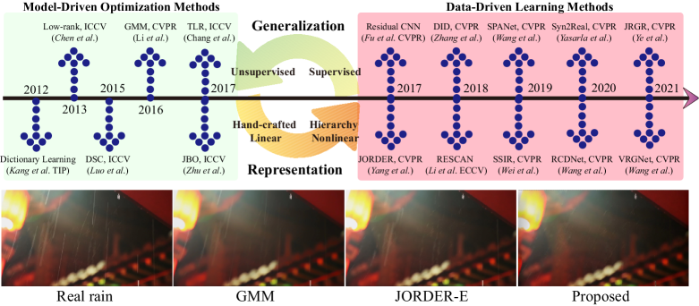
Figure 1. The complementary between the optimization and CNN methods. We show the development of typical rain streak removal methods. The unsupervised model driven-optimization methods generalize well yet with only shallow representation. On the contrary, the full/semi-supervised based CNN deraining methods are representative with poor generalization. In this work, we bridge the gap between the model-driven and data-driven methods within an end-to-end unsupervised learning framework. Below shows the real rain removal results for representative optimization-based GMM (Li et al., 2016), learning-based JORDER-E (Yang et al., 2019), and the proposed method.

In pre-deep learning era, the optimization methods have achieved considerable progress in rain streaks removal. The main idea of optimization model is to formulate deraining task into an image decomposition framework by decoupling the rain streaks and clean image components which lie on two distinguishable subspaces. Thus, the key of optimization model is to construct an energy function and manually design hand-crafted priors for each component. The dictionary learning (Kang et al., 2012; Luo et al., 2015), low-rank representation (Chen and Hsu, 2013; Chang et al., 2017), Gaussian mixture models (GMMs) (Li et al., 2016) have been widely explored for rain streaks removal. The optimization-based methods dig deeply into domain knowledge of the rain streaks, such as spatial sparsity (Kang et al., 2012; Gu et al., 2017), smoothness (Zhu et al., 2017a), non-local similarity (Chen and Hsu, 2013), directionality (Chang et al., 2017). Moreover, they are usually free from the large-scale training datasets, so they can generalize well for real rain streaks. However, these hand-crafted priors are typically based on linear transformation, in which the representation ability is limited, especially for highly complex and varied rainy scenes. In addition, the optimization procedure is usually slow due to the multiple iterations procedure.

Although the optimization-based methods have achieved promising deraining results, these hand-crafted priors are less robust to handle the rain streaks with diverse distributions, due to the varied angle, location, intensity, density, length, width and so on. In recent years, the deep learning based deraining methods (Fu et al., 2017; Yang et al., 2017; Zhang and Patel, 2018; Li et al., 2018, 2018; Ren et al., 2019; Wang et al., 2019; Wei et al., 2019; Hu et al., 2019; Li et al., 2019; Yang et al., 2019; Yasarla and Patel, 2019; Wang et al., 2019b; Zhu et al., 2019; Wang et al., 2019a; Li et al., 2019; Wang et al., 2020; Du et al., 2020; Yang et al., 2020; Deng et al., 2020; Jiang et al., 2020; Yasarla et al., 2020; Ye et al., 2021) have received tremendous success in deraining task due to nonlinear representation ability of CNN. The powerful representation enables the CNN to implicitly learn different complex distribution of the rain streaks. Another advantage of the CNN methods is the fast inference time once the network is trained. The key components in conventional CNN are to 1) prepare the training data pairs; 2) design architecture of the network; 3) define loss function for the training purpose.

Most of the existing CNN-based deraining methods are full-supervised, in which they pay most of their attention to the architecture design of the network such as the multi-stage (Yang et al., 2017; Li et al., 2018; Ren et al., 2019; Yang et al., 2019; Wang et al., 2020), multi-scale (Pang et al., 2020; Yasarla and Patel, 2019; Zhu et al., 2019; Jiang et al., 2020), attention (Li et al., 2018; Wang et al., 2019; Hu et al., 2019; Zhu et al., 2019), so as to better improve the representation for the rain streaks. The full-supervised deraining methods heavily rely on the paired clean and rainy image. The existing full-supervised methods usually construct a rain synthesis model to generate the simulated rainy image. However, there exist a huge gap between the real and synthetic rains. That is the main reason why the existing CNN methods have been less generalized for the real rain streaks. The semi-supervised deraining methods (Wei et al., 2019; Yasarla et al., 2020; Ye et al., 2021) could alleviate the generalization issue to some extent by introducing the real rainy image as the additional constraint. However, the problem still exists since these semi-supervised methods also employ the synthetic rainy image.

Overall, the model-driven optimization methods have good generalization endowed by the unsupervised loss yet weak representation (plane and linear) ability. On the contrary, the data-driven learning methods have good representation endowed by the hierarchy nonlinear transformation yet poor generalization (supervised loss on synthetic data) ability. This motivates us to inherit the powerful representation of the network and also the good generalization of optimization methods simultaneously.

In this work, we bridge the gap between the model-driven and data-driven methods within an end-to-end unsupervised learning framework. Specifically, we first discover a simple yet important domain knowledge that directional rain streak is anisotropic while the natural clean image is isotropic. This motivates us to construct a simple yet effective unsupervised directional gradient based optimization model (UDG) in which the rainy image is decomposed as the clean image regularized by isotropic TV and the rain streak constrained by anisotropic TV. UDG has good generalization yet poor representation ability and can be efficiently solved by the alternating direction method of multipliers (Lin et al., 2011). To further improve the representation of UDG, we design an UDG optimization model driven deep CNN (UDGNet). The architecture of the network mimics the main role of the optimization models with better feature representation. Consequently, the unsupervised loss of UDG is correspondingly enforced on UDGNet. Overall, the proposed method inherits good generalization and representation from both the optimization and CNN. The main contributions are summarized:

• Different from existing full/semi-supervised deraining methods, we attempt to solve real rain streaks from an unsupervised perspective. We connect the model-driven and data-driven methods via an unsupervised learning framework with simultaneous generalization and representation, which offers a new insight to deraining community.

• We discover the structural discrepancy between the rain streak and clean image. Consequently, we construct an unsupervised directional gradient based optimization model (UDG) for real rain streaks removal. Furthermore, we propose an optimization model-driven deep CNN (UDGNet) in which we optimize the network weights by minimizing the unsupervised loss function UDG.

• The proposed UDGNet can be trained with a few real rainy images, even one single image. We conduct extensive experiments on both synthetic and real-world datasets, which consistently perform superior against the state-of-the-art methods.

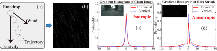
Figure 2. The illustration of the rain streaks and the statistical discrepancy between the rain streak and clean image. (a) The analysis of the physical procedure of the raindrop in real-world space. (b) The visualization of the rain streaks in imaging space. (c) and (d) show the gradient histogram of the clean image and rain streak, respectively.

2. Related Work

2.1. Optimization-based Deraining

The model-based optimization methods formulate the single image rain streaks removal task as an ill-posed problem, in which the decomposition framework is employed to model the image and rain streaks simultaneously with hand-crafted priors (Kang et al., 2012; Chen and Hsu, 2013; Luo et al., 2015; Li et al., 2016; Zhu et al., 2017a; Chang et al., 2017; Gu et al., 2017). The key of the optimization method is to dig the domain-knowledge of both the rain streaks and image. In 2012, Kang et al. (Kang et al., 2012) excavated the spatial sparsity of both the image and rain streaks, and first introduced the one-dimensional vector-based dictionary learning with morphological component analysis. Later, Luo et al. (Luo et al., 2015) proposed a discriminative sparse coding method by additionally forcing the two learned dictionaries with mutual exclusivity. Further, the authors utilized the non-local similarity of the images, and employed the two-dimensional low-rank matrix recovery (Chen and Hsu, 2013) to better preserve the structure of the images. The directional property of the rain streak has been widely utilized. For example, Chang et al. (Chang et al., 2017) proposed a transformed low-rank model for compact rain feature representation. Li et al. (Li et al., 2016) presented a simple patch-based Gaussian mixture models and can accommodate multiple orientations and scales of the rain streaks. In this work, we discover the structural discrepancy between the rain streak and clean image in the gradient domain, and propose a novel unsupervised directional gradient based optimization model for rain streaks removal. Moreover, we extend the proposed optimization model to the deep network by minimization of the unsupervised loss UDG, so as to significantly improve the feature representation for better real rain streaks removal.

2.2. Learning-based Deraining

The CNN based single image rain streak removal methods can be mainly classified into the following categories: full-supervised (Fu et al., 2017; Yang et al., 2017; Zhang and Patel, 2018; Li et al., 2018, 2018; Ren et al., 2019; Wang et al., 2019; Hu et al., 2019; Li et al., 2019; Yang et al., 2019; Yasarla and Patel, 2019; Wang et al., 2019b; Zhu et al., 2019; Wang et al., 2019a, 2020; Du et al., 2020; Yang et al., 2020; Deng et al., 2020; Jiang et al., 2020), semi-supervised (Wei et al., 2019; Yasarla et al., 2020), and unsupervised (Zhu et al., 2019). Most existing methods are full-supervised where the clean image and synthetic rain image pair are required. Fu et al. (Fu et al., 2017) first introduced the end-to-end residual CNN to solve the rain streaks removal problem. Yang et al. (Yang et al., 2017) jointly detected and removed the rain in a multi-task network. The multi-stage and multi-scale architecture networks (Li et al., 2018; Wang et al., 2020; Pang et al., 2020; Yasarla and Patel, 2019; Jiang et al., 2020) have been extensively studied for better feature representation. Ren et al. (Ren et al., 2019) proposed a simple yet effective progressive recurrent network with recursive blocks for image deraining. To better generalize the real rain streaks, the researchers employed the semi-supervised learning paradigm. For example, apart from the supervised loss, Wei et al. (Wei et al., 2019) additionally enforced a parameterized GMM distribution on real rain streaks. To get rid of the limitation of the paired synthetic-clean training data, the unsupervised methods (Zhu et al., 2019) have raised attention. The existing unsupervised methods all take advantage of the CycleGAN framework (Zhu et al., 2017b) to handle the unpaired real rain streaks. In this work, our method starts from the unpaired and unsupervised network. To the best of our knowledge, we are the first unsupervised network that handles the real rainy image from the loss function perspective by utilizing the domain knowledge of the rain streaks.

2.3. The Combination of Optimization and CNN

The model-driven optimization methods and the data-driven learning methods are the two main categories restoration methods over the past decades. These two methodologies are complementary to each other in terms of the generalization, representation, training and testing time. There are many attempts to combine them into a unified framework. The most popular way is the plug-and-play strategy (Zhang et al., 2017). Benefiting from the variable splitting techniques (Lin et al., 2011), the discriminative CNN can be plugged into model-based restoration methods as a learnable regularization. Liu et al. (Liu et al., 2018) exploited a deep layer prior under the maximum-a-posterior framework to recover the intrinsic rain structure. Another typical manner is the unfolding (Yang et al., 2016), which designs the network with sufficient interpretability by unfolding the iterative optimization procedure into a deep network architecture. Wang et al. (Wang et al., 2020) designed a rain convolutional dictionary RCDNet for image deraining with exact step-by-step corresponding relationship between the network modules and the operators in optimization procedure. In this work, we unify the optimization model and CNN into an end-to-end unsupervised learning network, in which we optimize the network weights by minimizing an unsupervised loss function, derived from the anisotropic smoothness knowledge of rain streaks. Moreover, the architecture of the model-driven deep neural network is interpretable with better feature representation.

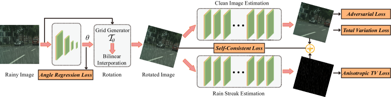
Figure 3. The architecture of the proposed network. The UDGNet mimics the main operations in optimization procedure. Given the rainy image, we first estimate the principal direction angle of the rain streaks and feed it to the simplified spatial transformation module (Jaderberg et al., 2015) so as to obtain the regular vertical rain streaks. Then, the rotated image is decomposed into distinguishable image and rain streak subspaces, which is realized by the domain knowledge driven unsupervised isotropic and directional anisotropic gradient loss. Finally, we reconstruct the rotated rainy image with the self-consistency loss to further improve the feature representation.

3. Methodology

3.1. Discrepancy Between Image and Rain Layer

The key of the unsupervised optimization method is to excavate the domain knowledge of both the clean image and rain streaks, so as to decouple the two components into distinguishable subspaces. The sparsity, low-rank, GMM properties have been extensively utilized in previous works. In this work, we discover a simple yet important domain knowledge that directional rain streak is anisotropic while the natural clean image is isotropic. Here, we provide an analysis to support our statement from a physical and image statistical viewpoint. On one hand, the physical shape of the rain is approximately spherical raindrop (Garg and Nayar, 2007). The raindrops are affected by both the gravity and wind. The gravity ensures that the rain is vertically descending and the wind determines the descending angle, as shown in Fig. 2(a). Then, the imaging system maps the raindrop of the real world to the image plane. Due to the long exposures of the imaging and fast motion of the raindrops, the visual appearance of the rain in image space is presented as severely motion-blurred rain streaks, as shown in Fig. 2(b). That is to say, the directional rain streaks are naturally anisotropic. On the contrary, the natural image is typically vertical and horizontal isotropic (Torralba and Oliva, 2003).

We further statistically demonstrate that the structure discrepancy between clean image and line-pattern rain streaks. Specifically, we first calculate the gradient maps (first-order forward difference) along both vertical and horizontal axis, and then calculate the histogram of gradient maps (x-axis denotes the gradient bins, y-axis represents the number count) on large-scale datasets, as shown in Fig. 2(c) and (d). The isotropic means that properties are the same when measured along axes in different directions. The gradient histograms of the image along different directions including x and y axis are very close to each other (isotropic TV), while this property does not hold true for the rain streaks (anisotropic TV). That is to say, the directional property of the rain streaks mainly increases the gradient variation across the streak line direction while has less influence along the streak line. The structure discrepancy between the clean image and the rain streak is the key to decouple them into two subspaces.

3.2. Unsupervised Directional Gradient Model

Now, the key problem is how to mathematically formulate the structure discrepancy into the optimization model. As for clean image, we utilize isotropic total variational to depict the isotropic gradient smoothness along both horizontal and vertical dimension. As for rain streak, we would like to design an anisotropic directional gradient constraint: penalize the gradient along the rain streak while preserving the gradient across rain streak. This is very reasonable, since the rain streaks exhibit obvious directionality similar to the sharp edges. However, the main difficulty is the arbitrary angle of rain streaks in different images. To solve this problem, we follow the rotated model in (Chang et al., 2017), so as to obtain vertical rain streaks:

(1) $$\theta\circ\textbf{\emph{Y}}=\textbf{\emph{X}}+\textbf{\emph{R}},$$

where Y is the observed rainy image, $\theta$ is the rotation angle, X is the clean background, and R is the rain streaks. The goal of this work is to estimate both clean image X and rain streaks R simultaneously from the given rainy image Y. The general optimization deraining model can be deduced via the maximum-a-posterior as follow:

(2) $$\mathop{min}\limits_{\textbf{\emph{X}},\textbf{\emph{R}}}\frac{1}{2}||\textbf{\emph{X}}+\textbf{\emph{R}}-\theta\circ\textbf{\emph{Y}}||_{F}^{2}+\tau P_{x}(\textbf{\emph{X}})+\lambda P_{r}(\textbf{\emph{R}}),$$

where the first term is the data fidelity, $P_{x}$ and $P_{r}$ denote the prior term on clean image and rain streaks, respectively. According to the analysis above, we choose the conventional isotropic TV for the clean image and anisotropic directional TV for the rain streaks. For simplicity of the optimization, we estimate the angle of the $\theta$ via TILT (Zhang et al., 2012) in advance, and denote $\textbf{\emph{Y}}_{r}=\theta\circ\textbf{\emph{Y}}$. Thus, the formulation of the unsupervised directional gradient image deraining model is:

(3) $$\mathop{min}\limits_{\textbf{\emph{X}},\textbf{\emph{R}}}\frac{1}{2}||\textbf{\emph{X}}+\textbf{\emph{R}}-\textbf{\emph{Y}}_{r}||_{F}^{2}+\tau||\textbf{\emph{X}}|{|_{\emph{TV}}}+\lambda||\textbf{\emph{R}}|{|_{\emph{UTV}}},$$

where $||\textbf{\emph{X}}|{|_{\emph{TV}}}=||\nabla\textbf{\emph{X}}||_{1}$ and $||\textbf{\emph{R}}|{|_{\emph{UTV}}}={||{\nabla_{x}}\textbf{\emph{R}}||_{1}+||{{\nabla_{y}}\textbf{\emph{Y}}_{r}-{\nabla_{y}}\textbf{\emph{R}}}||_{1}}$, and $\nabla=({\nabla_{x}};{\nabla_{y}})$ denotes the vertical (along the rain streak) and horizontal (across the rain streak) derivative operators, respectively, where $||\cdot|{|_{1}}$ denotes the sum of absolute value of the matrix elements.

1) Rain Streaks Update: given image X, the rain streaks R can be estimated from the following minimization problem:

(4)

Due to the non-differentiability of the ${L_{1}}$ norm, we introduce the ADMM (Lin et al., 2011) to convert the original problem into two easy subproblems with closed-form solutions. By introducing two auxiliary variables ${\textbf{\emph{P}}_{x}}={\nabla_{x}}\textbf{\emph{R}}$ and ${\textbf{\emph{P}}_{y}}={{\nabla_{y}}\textbf{\emph{R}}-{\nabla_{y}}\textbf{\emph{Y}}_{r}}$, the Eq. (4) is equivalent to following problem:

(5) $$\{\hat{\textbf{\emph{R}}},\hat{\textbf{\emph{P}}}_{x},\hat{\textbf{\emph{P}}}_{y}\}=\mathop{\arg\min}\limits_{\textbf{\emph{R}},{\textbf{\emph{P}}_{x}},{\textbf{\emph{P}}_{y}}}\frac{1}{2}||\textbf{\emph{X}}+\textbf{\emph{R}}-\textbf{\emph{Y}}_{r}||_{F}^{2}+\lambda_{x}||{\textbf{\emph{P}}_{x}}|{|_{1}}+\lambda_{y}||{\textbf{\emph{P}}_{y}}|{|_{1}}$$

$$+\frac{\alpha}{2}||{\textbf{\emph{P}}_{x}}-{\nabla_{x}}\textbf{\emph{R}}-\frac{{{\textbf{\emph{J}}_{x}}}}{\alpha}||_{F}^{2}+\frac{\beta}{2}||{\textbf{\emph{P}}_{y}}-({\nabla_{y}}\textbf{\emph{R}}-{\nabla_{y}}\textbf{\emph{Y}}_{r})-\frac{{{\textbf{\emph{J}}_{y}}}}{\beta}||_{F}^{2}.$$

$\blacksquare$ The R-related subproblem is

(6) $$\hat{\textbf{\emph{R}}}=\arg\mathop{\min}\limits_{\textbf{\emph{R}}} \frac{1}{2}||\textbf{\emph{X}}+\textbf{\emph{R}}-\textbf{\emph{Y}}_{r}||_{F}^{2}+\frac{\alpha}{2}||{\textbf{\emph{P}}_{x}}-{\nabla_{x}}\textbf{\emph{R}}-\frac{{{\textbf{\emph{J}}_{x}}}}{\alpha}||_{F}^{2}$$

$$+\frac{\beta}{2}||{\textbf{\emph{P}}_{y}}-({\nabla_{y}}\textbf{\emph{R}}-{\nabla_{y}}\textbf{\emph{Y}}_{r})-\frac{{{\textbf{\emph{J}}_{y}}}}{\beta}||_{F}^{2},$$

which has a close-form solution via 2-D fast Fourier transform (FFT)

(7)

$\blacksquare$ The $\{\textbf{\emph{P}}_{x},\textbf{\emph{P}}_{y}\}$-related subproblem is

(8) $$\left\{{\begin{array}[]{*{20}{c}}{\hat{\textbf{\emph{P}}_{x}}=\arg\mathop{\min}\limits_{\textbf{\emph{P}}_{x}}\lambda_{x}||\textbf{\emph{P}}_{x}|{|_{1}}+\frac{\alpha}{2}||\textbf{\emph{P}}_{x}-\nabla_{x}\textbf{\emph{R}}-\frac{\textbf{\emph{J}}_{x}}{\alpha}||_{F}^{2}}\\ \leavevmode\resizebox{394.59247pt}{}{${\hat{\textbf{\emph{P}}_{y}}=\arg\mathop{\min}\limits_{\textbf{\emph{P}}_{y}}\lambda_{y}||\textbf{\emph{P}}_{y}|{|_{1}}+\frac{\beta}{2}||\textbf{\emph{P}}_{y}-({\nabla_{y}}\textbf{\emph{R}}-{\nabla_{y}}\textbf{\emph{Y}}_{r})-\frac{\textbf{\emph{J}}_{y}}{\beta}||_{F}^{2}}.$}\end{array}}\right.$$

which can be solved efficiently via a soft shrinkage operator:

(9) $$\left\{{\begin{array}[]{*{30}{c}}{{\textbf{\emph{P}}_{x}^{k+1}}=shrink\_{\emph{L}_{1}}(\nabla_{x}{\textbf{\emph{R}}^{k+1}}+\frac{{{\textbf{\emph{J}}_{x}^{k}}}}{\alpha^{k}},\frac{\lambda_{x}}{\alpha^{k}})}\\ {{\textbf{\emph{P}}_{y}^{k+1}}=shrink\_{\emph{L}_{1}}(\nabla_{y}{\textbf{\emph{R}}^{k+1}}-{\nabla_{y}}\textbf{\emph{Y}}_{r}+\frac{{{\textbf{\emph{J}}_{y}^{k}}}}{\beta^{k}},\frac{\lambda_{y}}{\beta^{k}})}\\ {shrink\_{\emph{L}_{1}}(r,\xi)=\frac{r}{{|r|}}*\max(|r|-\xi,0).}\end{array}}\right.$$

Finally, the Lagrangian multipliers and penalization parameters are updated as follows:

(10) $$\left\{{\begin{array}[]{*{30}{c}}{\textbf{\emph{J}}_{x}^{k+1}}={\textbf{\emph{J}}_{x}^{k}}+{\alpha^{k}}(\nabla_{x}{\textbf{\emph{R}}^{k+1}}-{\textbf{\emph{P}}_{x}^{k+1}})\\ {\textbf{\emph{J}}_{y}^{k+1}}={\textbf{\emph{J}}_{y}^{k}}+{\beta^{k}}(\nabla_{y}{\textbf{\emph{R}}^{k+1}}-\nabla_{y}{\textbf{\emph{Y}}_{r}}-{\textbf{\emph{P}}_{y}^{k+1}})\\ \{{\alpha^{k+1}},{\beta^{k+1}}\}=\{{\alpha^{k}},{\beta^{k}}\}\cdot\rho.\end{array}}\right.$$

2) Image Update: given rain streak R, the image X can be estimated from the following minimization problem:

(11) $$\hat{\textbf{\emph{X}}}=\arg\mathop{\min}\limits_{\textbf{\emph{X}}}\frac{1}{2}||\textbf{\emph{X}}+\textbf{\emph{R}}-\textbf{\emph{Y}}_{r}||_{F}^{2}+\tau||{\nabla}\textbf{\emph{X}}|{|_{1}}.$$

The optimization of Eq. (11) is similar to that of Eq. (4). Here, we do not describe the procedure in detail.

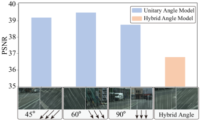
Figure 4. The advantage of rotation for rainy images. The same model trained on the unitary rain streak angle dataset significantly outperforms that of the hybrid angle.

3.3. The Optimization Model-driven Deep CNN

Although the UDG could remove most of the rain streaks and well accommodate different rainy images, the residual rain streaks and over-smooth phenomenon are easily observed, especially for the complex scenes. The main reason is the limited representation ability of the hand-crafted linear transformation of TV prior. In this work, we bridge the gap between the optimization model and the deep CNN to overcome this issue.

From the optimization model perspective, we deepen the shallow optimization model by introducing deep CNN with powerful representation ability. Specifically, we introduce CNN to approximate clean image and rain streaks, and enforce the unsupervised loss of optimization model as constraint for the deep CNN. Thus, the unsupervised learning framework can retain generalization ability, meanwhile leverage the hierarchy nonlinear representation of CNN.

From the deep learning perspective, we replace the conventional supervised paired constraint by the unsupervised loss of the optimization model. Thus, we get rid of the paired clean-synthetic labels for supervised training and directly train from the real rainy images. The unsupervised loss endows us the good generalization ability with powerful representation of the network. Moreover, most of the optimization methods are time-consuming, since the iteration of the solving large-scale linear systems are required. Thus, the proposed method can enjoy a fast inference speed of CNN.

The Architecture and Loss of UDGNet. Now we introduce concrete architecture of the proposed network which is used for minimizing the defined unsupervised loss function. The overall network architecture in Fig. 3 is to mimic the optimization procedure of Eq. (2). Specifically, we first learn the rotation angle $\theta$ regression module which repeatedly includes several conv and pooling layers.

(12) $${\mathcal{L}_{{\theta}}={\left\|{{\theta}-\mathcal{F}\left(\textbf{\emph{Y}};\textbf{\emph{W}}_{\theta}\right)}\right\|}_{{2}}},$$

where Y is the input rainy image, $\mathcal{F}(\bullet)$ is the network transformation and $\textbf{\emph{W}}_{\theta}$ is the learnable angle regression parameters, and ${\theta}$ is ground-truth of the rain streaks which can be easily obtained in advance. Compared with the 2D image and rain streak, the angle is a single scalar, which is much easier to learn and label.

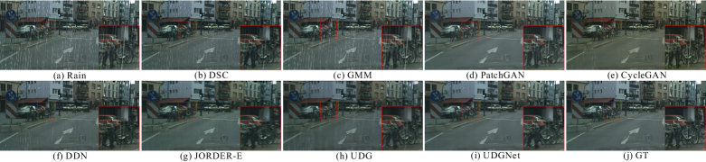
Figure 5. Visualization of deraining results on Cityscape dataset.

Figure 6. Visualization of deraining results on Rain1400 dataset.

Table 1. Quantitative comparison PSNR and SSIM with state-of-the-art methods on synthetic datasets.

Dataset	Index	Rain	Optimization			Full-supervised			Semi	Unsupervised
			DSC	GMM	UDG	DDN	JORDER-E	RCDNet	SSIR	GAN	Cyclegan	UDGNet
Cityscape	PSNR	26.22	28.18	29.11	26.95	30.59	24.76	28.87	25.15	30.09	31.62	34.65
	SSIM	0.7776	0.8104	0.8649	0.9434	0.9232	0.8559	0.8778	0.8165	0.9325	0.9140	0.9653
Rain1400	PSNR	23.68	26.26	25.72	23.35	28.07	22.18	24.69	25.67	24.14	28.32	29.16
	SSIM	0.7542	0.7828	0.7797	0.8380	0.8633	0.7719	0.7840	0.8183	0.7880	0.8685	0.8910

Next, we feed the learned scalar angle into a modified differentiable spatial transform module (Jaderberg et al., 2015), which explicitly allows the spatial affine transformation of the input image. The classical STN (Jaderberg et al., 2015) can not control how the transformed feature map is. Compared with the classical STN, we additionally enforce a physical meaning rotation angle ${\theta}$, so that the rainy image Y with arbitrary direction can be well rectified into the vertical direction $\textbf{\emph{Y}}_{r}$. We show the original image Y and the rotated version $\textbf{\emph{Y}}_{r}$, in Fig. 3. Such a simple operation would significantly reduce the rain streak removal difficulty by reducing the angle variations of different rain streaks. To show the effectiveness of the rotation, we train on two cases: rain streaks with arbitrary directions and rain streaks with only the vertical direction. The results are reported in Fig. 4, which is not surprising since the rotation has explicitly eliminated the uncertainty.

Then, we construct two parallel streams for the image and rain streaks estimation, analog to the two prior terms $P_{x}(\textbf{\emph{X}})$ and $P_{r}(\textbf{\emph{R}})$ in Eq. (2). Each stream corresponds to the alternating minimization of Eq. (4) and Eq. (11) in optimization model. Furthermore, we additionally introduce the adversarial loss (Goodfellow et al., 2014) on the clean image for better textures preserving. The architecture of the two streams are the same with 32 Resblocks (He et al., 2016). Thus, instead of directly minimization of the clean image and the rain streaks, we learn the parameters $\textbf{\emph{W}}_{I}$ and $\textbf{\emph{W}}_{R}$ in each stream as follow:

(13) $${\mathcal{L}_{{image}}=\tau{\left\|{\nabla\mathcal{F}\left(\textbf{\emph{Y}}_{{r}};\textbf{\emph{W}}_{{I}}\right)}\right\|}_{{1}}}+\mu\mathcal{L}_{adv},$$

(14)

where $\mathcal{F}(\bullet)$ is the network transformation, $\mathcal{L}_{adv}$ is the adversarial loss (Goodfellow et al., 2014). The first term TV loss in Eq. (13) serves as the local pixel-level smoothness prior while the second term adversarial loss works as the global image-level statistical prior. The two terms are complementary to each other, so as to obtain natural and clean image.

Finally, we enforce the self-consistency constraint by composing the estimated image and rain streaks back to the rotated rainy image, which is exactly the first data fidelity term in Eq. (2):

(15) $${\mathcal{L}_{{self}}={\left\|{\textbf{\emph{Y}}_{{R}}-\mathcal{F}\left(\textbf{\emph{Y}}_{r};\textbf{\emph{W}}_{I}\right)-\mathcal{F}\left(\textbf{\emph{Y}}_{r};\textbf{\emph{W}}_{R}\right)}\right\|}_{{2}}}.$$

Thus, the overall loss of the proposed network can be interpreted as:

(16) $$\mathcal{L}_{{overall}}=\mathcal{L}_{{\theta}}+\mathcal{L}_{{image}}+\mathcal{L}_{{rain}}+\mathcal{L}_{{self}}.$$

The deep network explicitly learns the optimization procedure, in which each module and loss mimic the main operation in optimization. On one hand, the network inherits the unsupervised domain knowledge from optimization. Thus, the proposed network generalizes well to different rainy images and can be trained and tested on one single image (without the adversarial loss). Moreover, once the network is trained, it only requires a very fast forward pass through the deep network to predict the clean image without further optimization steps. On the other hand, the proposed model is representative of the complex scenes endowed by the highly-nonlinear network, and the proposed network is interpretable and controllable.

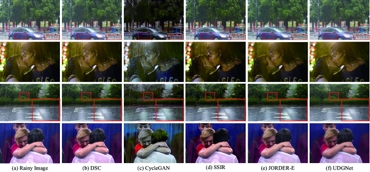
Figure 7. Visualization of deraining results on RealRain dataset.

Table 2. Quantitative comparison NIQE and User study results with state-of-the-art methods on real dataset.

Method	Rainy	DSC	GMM	UDG
NIQE	5.70	5.55	6.06	5.12
User study	1.00	2.88	3.64	4.53
Method	JORDER-E	RCDNet	CycleGAN	UDGNet
NIQE	5.48	5.62	6.54	5.08
User study	4.03	3.03	1.14	5.69

4. EXPERIMENTAL RESULTS

4.1. Datasets and Experimental Setting

Datasets. We evaluate UDGNet on both synthetic and real datasets.

• Cityscape. We simulate cityscapes rain images following the screen blend model (Luo et al., 2015) with different streak length, width, angle and intensity. We follow the cityscapes dataset with 2975 images for training and 500 images for testing.

• Rain1400. We adopt rain1400 (Fu et al., 2017) as another synthetic dataset, which contains 1400 rain/clear images pairs. We randomly select 12600 for training and 1400 pairs for testing.

• RealRain. We collect real world rainy images with large field of view from the datasets (Yang et al., 2017; Wei et al., 2019; Chen et al., 2018) and Google search. We utilize 100 real rainy images to train and test the UDGNet.

Table 3. Model size (MB) and time complexity (seconds)

Method	DSC	GMM	UDG	DDN
Model size	-	-	-	0.233
Running time	5066	1443	7.846	0.162
Method	JORDER-E	RCDNet	CycleGAN	UDGNet
Model size	16.7	13.1	11.7	5.7
Running time	9.123	22.6	3.098	0.129

Implemention Details. The images are trained and tested through sliding windows with the size of 128*128. The angle of rain streaks is obtained via the TILT (Zhang et al., 2012) in advance for training. We adopt Adam (Kingma and Ba, 2015) as the optimizer with batch size of 8. The initial learning rate is set to be 0.001 and decay 0.1 every 30 epochs. We set the hyper-parameter $\tau$, $\mu$, $\lambda_{x}$, $\lambda_{y}$ as 0.01, 400, 1.5, 1.0, respectively.

Experimental Setting. We compare the proposed unsupervised UDG and UDGNet with (1) optimization methods DSC (Luo et al., 2015) and GMM (Li et al., 2016); (2) supervised methods DDN (Fu et al., 2017), JORDER-E (Yang et al., 2019) and RCDNet (Wang et al., 2020); (3) semi-supervised methods SSIR (Wei et al., 2019); (4) unsupervised network PatchGAN (Isola et al., 2017) and CycleGAN (Zhu et al., 2017b). For synthetic data, the full-reference PSNR and SSIM are utilized as the quantitative evaluation. For real-world images, we employ the non-reference NIQE (Mittal et al., 2013) and user studies to quantitatively evaluate the visual quality of deraining results. The higher PSNR, SSIM and user study point is and the lower the NIQE is, the better the deraining result is. The optimization methods do not need the training dataset. The supervised methods are trained on the defined dataset in the original paper and tested on different datasets in our work.

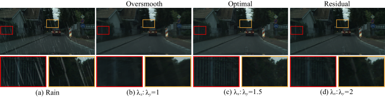
Figure 8. The illustration of how the regularization parameters control the deraining strength.

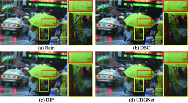
Figure 9. The single image training and inferencing.

Table 4. The influence of the estimated angle $\theta$.

$\theta$	Estimated	GT	GT$\pm$5∘	GT$\pm$10∘	GT$\pm$20∘
PSNR	34.65	34.71	34.56	34.26	33.03
SSIM	0.9663	0.9665	0.9639	0.9602	0.9389

4.2. Quantitative and Qualitative Results

Qualitative Results. In Fig. 5-7, we show the visual deraining results on both synthetic and real datasets: Cityscape, Rain1400 and RealRain. We can observe that there are obvious residual rain streaks in optimization-based methods, especially in Fig. 5, because of the limited representation ability of hand-crafted priors for diverse background and rain streaks. The unsupervised learning-based methods PatchGAN and CycleGAN could remove most of the rain streaks with a few residual. However, GAN-based unsupervised methods are difficult to train and easy to collapse, since they heavily rely on the distribution of training dataset. The supervised methods DDN and JORDER-E could suppress rain streaks to some extent, while there are also some residual rain streaks in the results due to the data distribution discrepancy. The optimization model UDG could remove most rain streaks. UDGNet further enhances the performance. On one hand, the visual rain streaks have been satisfactorily removed by the UDGNet with few residuals. On the other hand, compared with the UDG, the unsupervised learning-based UDGNet could well preserve the image structures. Compared with other methods, the proposed UDGNet could achieve better performance in terms of both rain streaks removal and image texture preserving.

Table 5. The effectiveness analysis of each loss in UDGNet.

Case	$\mathcal{L}_{img-tv}$	$\mathcal{L}_{img-adv}$	$\mathcal{L}_{rain}$	$\mathcal{L}_{self}$	PSNR	SSIM
1	$\surd$	$\times$	$\times$	$\times$	22.63	0.8229
2	$\times$	$\surd$	$\times$	$\times$	30.09	0.9325
3	$\surd$	$\surd$	$\times$	$\times$	30.08	0.8915
4	$\times$	$\times$	$\surd$	$\times$	32.44	0.9538
5	$\times$	$\surd$	$\surd$	$\surd$	33.01	0.9681
6	$\surd$	$\times$	$\surd$	$\surd$	34.64	0.9644
7	$\surd$	$\surd$	$\surd$	$\surd$	34.65	0.9653

Quantitative Results. The quantitative results are reported in Table 1 and 2 in which the best results are in bold. The UDGNet consistently obtains the best deraining results, which further demonstrates the superior of the proposed method in terms of the performance and generalization. We further show model size and time complexity of different methods in Table 3. The proposed UDGNet is computationally cheap and efficient. The model size of UDGNet is about 5.7MB, which is significantly smaller than the competing methods. Furthermore, we benchmark the running time with an Intel Core i7-8700 CPU and an NVIDIA RTX 2080Ti. For an image with size 1024*2048, the running time of the UDG is 7.8s, which is obviously faster than DSC (5066s) and GMM (1433s). The testing time of UDGNet is 0.12s, which is more attractive for practical use.

4.3. Ablation Study

How does Angle Estimation Affect the Performance? The angle estimation and rotation module is an important pre-processing part of our UDGNet. In Table 4, we show how the angle estimation influences the deraining performance. We can observe that the more accurate the angle is, the better the deraining result is, which indicates that precise angle guidance can indeed improve UDGNet for better deraining performance. Moreover, the deraining result of the estimated angle is very close to that of the provided the oracle (GT) angle, which validates the effectiveness of the proposed network.

What is the Effectiveness of Each Loss? To verify the effect of each loss in UDGNet, in Table 5, we conduct ablation study of each term on cityscape validation. From cases 1, 2, 3: the adversarial loss is more important than the TV loss for image. From case 4: the proposed directional domain knowledge of rain streak is very effective for rain removal. From case 5, 6, 7: the joint loss with both rain streak and clean image could further boost the performance. Moreover, the self-consistency loss is also beneficial to the performance.

How Can We Control the Deraining Result of UDGNet? The loss function of UDGNet is derived from optimization model (UDG), in which each term has clear interpretability. Thus the deraining strength can be controlled through hyper-parameters $\lambda_{x}$ and $\lambda_{y}$. As shown in Fig. 8, different deraining results are obtained with different $\lambda_{x}/\lambda_{y}$ ratios. As ratio increases, more details are preserved with more streaks left, and vice versa. Thus, we can set different ratios to balance texture preservation and rain streak removal adaptively.

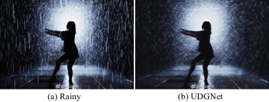
Figure 10. The limitation of the UDGNet.

4.4. Discussion

Single Image Training and Inference The previous learning based methods consistently need a number of the training samples, in which the testing performance heavily relies on the training datasets. In this work, our unsupervised learning framework not only utilizes external dataset but also the internal prior knowledge of singe image. Therefore, the UDGNet can be trained on both the large scale datasets and one single image. We test the performance of single image training along with the similar deep image prior DIP (Ulyanov et al., 2018) for comparison in Fig. 9. We can observe that the UDGNet could well remove and rain streaks with clear image texture, while the DIP has unexpectedly over-smooth the image details.

Limitation In Fig. 10, we show a real image with rain streaks (nearby) and veiling artifacts (distant). We can observe that the rain streaks have been satisfactorily removed while the veiling effects still exist in the result. This is reasonable, since the UDGNet mainly utilizes the directional anisotropic characteristic in the loss. In future, we would like to incorporate the domain knowledge of the veiling artifacts via the unsupervised loss into the proposed framework.

5. Conclusion

In this work, we aim at the real image rain streak removal, and propose a novel optimization model driven deep CNN method for unsupervised deraining. Our start point is to bridge the gap between the model-driven optimization method and the data-driven learning method in terms of the generalization and representation. The key to our learning framework is the modelling of the structure discrepancy between the rain streak and clean image. We formulate this domain knowledge into unsupervised direction gradient optimization model, and transfer the unsupervised loss function to the deep network, such that the proposed method could simultaneously achieve good generalization and representation ability. Extensive experimental results on both the real and synthetic datasets demonstrate the effectiveness of the proposed method for real rain streaks removal.

Acknowledgements.This work was supported by National Natural Science Foundation of China under Grant No. 61971460, China Postdoctoral Science Foundation under Grant 2020M672748, National Postdoctoral Program for Innovative Talents BX20200173 and Equipment Pre-Research Foundation under grant No. 6142113200304.

References

- (1)
- Chang et al. (2017) Yi Chang, Luxin Yan, and Sheng Zhong. 2017. Transformed low-rank model for line pattern noise removal. In Proc. ICCV. 1726–1734.
- Chen et al. (2018) Jie Chen, Cheen-Hau Tan, Junhui Hou, Lap-Pui Chau, and He Li. 2018. Robust video content alignment and compensation for rain removal in a CNN framework. In Proc. CVPR. 6286–6295.
- Chen and Hsu (2013) Yi Lei Chen and Chiou Ting Hsu. 2013. A generalized low-rank appearance model for spatio-temporally correlated rain streaks. In Proc. ICCV. 1968–1975.
- Deng et al. (2020) Sen Deng, Mingqiang Wei, Jun Wang, Yidan Feng, Luming Liang, Haoran Xie, Fulee Wang, and Meng Wang. 2020. Detail-recovery Image Deraining via Context Aggregation Networks. In Proc. CVPR. 14560–14569.
- Du et al. (2020) Yingjun Du, Jun Xu, Xiantong Zhen, Ming-Ming Cheng, and Ling Shao. 2020. Conditional Variational Image Deraining. IEEE Trans. Image Process. 29 (2020), 6288–6301.
- Fu et al. (2017) Xueyang Fu, Jiabin Huang, Delu Zeng, Yue Huang, Xinghao Ding, and John Paisley. 2017. Removing rain from single images via a deep detail network. In Proc. CVPR. 3855–3863.
- Garg and Nayar (2007) Kshitiz Garg and Shree K Nayar. 2007. Vision and rain. Int. J. Comput. Vision 75, 1 (2007), 3–27.
- Goodfellow et al. (2014) Ian J Goodfellow, Jean Pouget-Abadie, Mehdi Mirza, Bing Xu, David Warde-Farley, Sherjil Ozair, Aaron Courville, and Yoshua Bengio. 2014. Generative Adversarial Networks. In Proc. NIPS. 2672–2680.
- Gu et al. (2017) Shuhang Gu, Deyu Meng, Wangmeng Zuo, and Lei Zhang. 2017. Joint convolutional analysis and synthesis sparse representation for single image layer separation. In Proc. ICCV. 1708–1716.
- He et al. (2016) Kaiming He, Xiangyu Zhang, Shaoqing Ren, and Jian Sun. 2016. Deep residual learning for image recognition. In Proc. CVPR. 770–778.
- Hu et al. (2019) Xiaowei Hu, Chi-Wing Fu, Lei Zhu, and Pheng-Ann Heng. 2019. Depth-attentional Features for Single-image Rain Removal. In Proc. CVPR. 8022–8031.
- Isola et al. (2017) Phillip Isola, Jun-Yan Zhu, Tinghui Zhou, and Alexei A. Efros. 2017. Image-to-Image Translation with Conditional Adversarial Networks. In Proc. CVPR. 1125–1134.
- Jaderberg et al. (2015) Max Jaderberg, Karen Simonyan, Andrew Zisserman, and Koray Kavukcuoglu. 2015. Spatial transformer networks. In Proc. ICLR.
- Jiang et al. (2020) Kui Jiang, Zhongyuan Wang, Peng Yi, Chen Chen, Baojin Huang, Yimin Luo, Jiayi Ma, and Junjun Jiang. 2020. Multi-Scale Progressive Fusion Network for Single Image Deraining. In Proc. CVPR. 8346–8355.
- Kang et al. (2012) LiWei Kang, ChiaWen Lin, and YuHsiang Fu. 2012. Automatic single-image-based rain streaks removal via image decomposition. IEEE Trans. Image Process. 21, 4 (2012), 1742–1755.
- Kingma and Ba (2015) Diederik P Kingma and Jimmy Ba. 2015. Adam: A Method for Stochastic Optimization. In Proc. ICLR.
- Li et al. (2018) Guanbin Li, Xiang He, Wei Zhang, Huiyou Chang, Le Dong, and Liang Lin. 2018. Non-locally Enhanced Encoder-Decoder Network for Single Image De-raining. In ACM. MM. 1056–1064.
- Li et al. (2019) Ruoteng Li, Loong-Fah Cheong, and Robby T Tan. 2019. Heavy Rain Image Restoration: Integrating Physics Model and Conditional Adversarial Learning. In Proc. CVPR. 1633–1642.
- Li et al. (2019) Siyuan Li, Wenqi Ren, Jiawan Zhang, Jinke Yu, and Xiaojie Guo. 2019. Single image rain removal via a deep decomposition–composition network. Comput. Vis. Image Und. 186, 6 (2019), 48–57.
- Li et al. (2018) Xia Li, Jianlong Wu, Zhouchen Lin, Hong Liu, and Hongbin Zha. 2018. Recurrent squeeze-and-excitation context aggregation net for single image deraining. In Proc. ECCV. 254–269.
- Li et al. (2016) Yu Li, Robby T Tan, Xiaojie Guo, Jiangbo Lu, and Michael S Brown. 2016. Rain streak removal using layer priors. In Proc. CVPR. 2736–2744.
- Lin et al. (2011) Zhouchen Lin, Risheng Liu, and Zhixun Su. 2011. Linearized alternating direction method with adaptive penalty for low-rank representation. In NIPS. 612–620.
- Liu et al. (2018) Risheng Liu, Zhiying Jiang, Long Ma, Xin Fan, and Zhongxuan Luo. 2018. Deep Layer Prior Optimization for Single Image Rain Streaks Removal. In Proc. ICASSP. 1408–1412.
- Luo et al. (2015) Yu Luo, Yong Xu, and Hui Ji. 2015. Removing rain from a single image via discriminative sparse coding. In Proc. ICCV. 3397–3405.
- Mittal et al. (2013) Anish Mittal, Rajiv Soundararajan, and Alan C. Bovik. 2013. Making a ’Completely Blind’ Image Quality Analyzer. IEEE Signal Proc. Let. 20, 3 (2013), 209–212.
- Pang et al. (2020) Bo Pang, Deming Zhai, Junjun Jiang, and Xianming Liu. 2020. Single Image Deraining via Scale-space Invariant Attention Neural Network. In ACM. MM. 375–383.
- Redmon and Farhadi (2017) Joseph Redmon and Ali Farhadi. 2017. YOLO9000: better, faster, stronger. In Proc. CVPR. 7263–7271.
- Ren et al. (2019) Dongwei Ren, Wangmeng Zuo, Qinghua Hu, Pengfei Zhu, and Deyu Meng. 2019. Progressive image deraining networks: a better and simpler baseline. In Proc. CVPR. 3937–3946.
- Torralba and Oliva (2003) Antonio Torralba and Aude Oliva. 2003. Statistics of natural image categories. Network: computation in neural systems 14, 3 (2003), 391–412.
- Ulyanov et al. (2018) Dmitry Ulyanov, Andrea Vedaldi, and Victor Lempitsky. 2018. Deep image prior. In Proc. CVPR. 9446–9454.
- Wang et al. (2019b) Guoqing Wang, Changming Sun, and Arcot Sowmya. 2019b. ERL-Net: Entangled Representation Learning for Single Image De-Raining. In Proc. ICCV. 5644–5652.
- Wang et al. (2020) Hong Wang, Qi Xie, Qian Zhao, and Deyu Meng. 2020. A Model-driven Deep Neural Network for Single Image Rain Removal. In Proc. CVPR. 3103–3112.
- Wang et al. (2019) Tianyu Wang, Xin Yang, Ke Xu, Shaozhe Chen, Qiang Zhang, and Rynson WH Lau. 2019. Spatial Attentive Single-Image Deraining with a High Quality Real Rain Dataset. In Proc. CVPR. 12270–12279.
- Wang et al. (2019a) Zheng Wang, Jianwu Li, and Ge Song. 2019a. DTDN: Dual-task De-raining Network. In ACM. MM. 1833–1841.
- Wei et al. (2019) Wei Wei, Deyu Meng, Qian Zhao, Zongben Xu, and Ying Wu. 2019. Semi-Supervised Transfer Learning for Image Rain Removal. In Proc. CVPR. 3877–3886.
- Yang et al. (2019) W. Yang, R. Tan, J. Feng, Z. Guo, S. Yan, and J. Liu. 2019. Joint rain detection and removal from a single image with contextualized deep networks. IEEE Trans. Pattern Anal. Mach. Intell. 42, 6 (2019), 1377–1393.
- Yang et al. (2017) Wenhan Yang, Robby T Tan, Jiashi Feng, Jiaying Liu, Zongming Guo, and Shuicheng Yan. 2017. Deep joint rain detection and removal from a single image. In Proc. CVPR. 1357–1366.
- Yang et al. (2020) Wenhan Yang, Robby T. Tan, Shiqi Wang, Yuming Fang, and Jiaying Liu. 2020. Single Image Deraining: From Model-Based to Data-Driven and Beyond. IEEE Trans. Pattern Anal. Mach. Intell. (2020).
- Yang et al. (2016) Yan Yang, Jian Sun, Huibin Li, and Zongben Xu. 2016. Deep ADMM-Net for compressive sensing MRI. In Proc. NIPS. 10–18.
- Yasarla and Patel (2019) Rajeev Yasarla and Vishal M. Patel. 2019. Uncertainty Guided Multi-Scale Residual Learning-Using a Cycle Spinning CNN for Single Image De-Raining. In Proc. CVPR. 8405–8414.
- Yasarla et al. (2020) Rajeev Yasarla, Vishwanath A. Sindagi, and Vishal M Patel. 2020. Syn2Real Transfer Learning for Image Deraining using Gaussian Processes. In Proc. CVPR. 2726–2736.
- Ye et al. (2021) Yuntong Ye, Yi Chang, Hanyu Zhou, and Luxin Yan. 2021. Closing the Loop: Joint Rain Generation and Removal via Disentangled Image Translation. In Proc. CVPR.
- Zhang and Patel (2018) He Zhang and Vishal M Patel. 2018. Density-aware single image de-raining using a multi-stream dense network. In Proc. CVPR. 695–704.
- Zhang et al. (2017) Kai Zhang, Wangmeng Zuo, Shuhang Gu, and Lei Zhang. 2017. Learning deep CNN denoiser prior for image restoration. In Proc. CVPR. 3929–3938.
- Zhang et al. (2012) Zhengdong Zhang, Arvind Ganesh, Xiao Liang, and Yi Ma. 2012. TILT: Transform invariant low-rank textures. Int. J. Comput. Vision 99, 1 (2012), 1–24.
- Zhao et al. (2017) Hengshuang Zhao, Jianping Shi, Xiaojuan Qi, Xiaogang Wang, and Jiaya Jia. 2017. Pyramid scene parsing network. In Proc. CVPR. 2881–2890.
- Zhu et al. (2019) Hongyuan Zhu, Xi Peng, Tianyi Zhou, Songfan Yang, Vijay Chanderasekh, Liyuan Li, and Joo-Hwee Lim. 2019. Single Image Rain Removal with Unpaired Information: A Differentiable Programming Perspective. In Proc. AAAI. 9332–9339.
- Zhu et al. (2017b) Jun-Yan Zhu, Taesung Park, Phillip Isola, and Alexei A. Efros. 2017b. Unpaired Image-to-Image Translation using Cycle-Consistent Adversarial Networks. In Proc. CVPR. 2223–2232.
- Zhu et al. (2017a) Lei Zhu, ChiWing Fu, Dani Lischinski, and PhengAnn Heng. 2017a. Joint bi-layer optimization for single-image rain streak removal. In Proc. ICCV. 2526–2534.