The TerraByte Client: providing access to terabytes of plant data

Abstract

In this paper we demonstrate the TerraByte Client, a software to download user-defined plant datasets from a data portal hosted at Compute Canada. To that end the client offers two key functionalities: (1) It allows the user to get an overview on what data is available and a quick way to visually check samples of that data. For this the client receives the results of queries to a database and displays the number of images that fulfill the search criteria. Furthermore, a sample can be downloaded within seconds to confirm that the data suits the user’s needs. (2) The user can then download the specified data to their own drive. This data is prepared into chunks server-side and sent to the user’s end-system, where it is automatically extracted into individual files. The first chunks of data are available for inspection after a brief waiting period of a minute or less depending on available bandwidth and type of data. The TerraByte Client has a full graphical user interface for easy usage and uses end-to-end encryption. The user interface is built on top of a low-level client. This architecture in combination of offering the client program open-source makes it possible for the user to develop their own user interface or use the client’s functionality directly. An example for direct usage could be to download specific data on demand within a larger application, such as training machine learning models.

Availability

The TerraByte Client is available at the TerraByte homepage https://terrabyte.acs.uwinnipeg.ca/resources.html.

I Introduction

Digital agriculture is an upcoming field with the goal of using modern technologies such as robotics, phenotyping, and machine learning to advance and transform the way we grow food [1, 2, 3, 4, 5, 6, 7]. The vision of autonomous agents making plant-by-plant decisions within the field motivates this research. However, we often encounter, especially in the area of machine learning, a bottleneck of labelled data on which models can be trained and improved upon [8, 9]. Labelled data, at a minimum, is the data itself (for example an image) plus information about what the data represents (for example the label “Soybean” attached to an image). Often, the information provided – metadata – goes beyond simple labelling (for example also tracking the age of the Soybean plant, time and day of imaging, geolocation, etc.). In machine learning, for example with convolutional neural networks (CNN), we require thousands if not hundreds of thousands of labelled images to perform well. Labelled data is often created by manually labelling existing datasets and scaled to millions of images by crowdsourcing the efforts [10, 11, 12]. However, in the case of plant identification, the knowledge required for accurate labelling is more complex and uncommon and thus this approach of crowdsourcing is not available.

Still, when looking at similar applications we can expect strong results, once the challenge of having labelled image-data is resolved. CNNs have been applied very successfully in image-classification tasks with results that eventually outperformed human-level accuracy (see for example [13, 14, 15]). What these models have in common is that they were trained upon a vast amount of image data. The most prominent of these datasets being ImageNet [16, 17], which consists of more than 1.2 million labelled images.

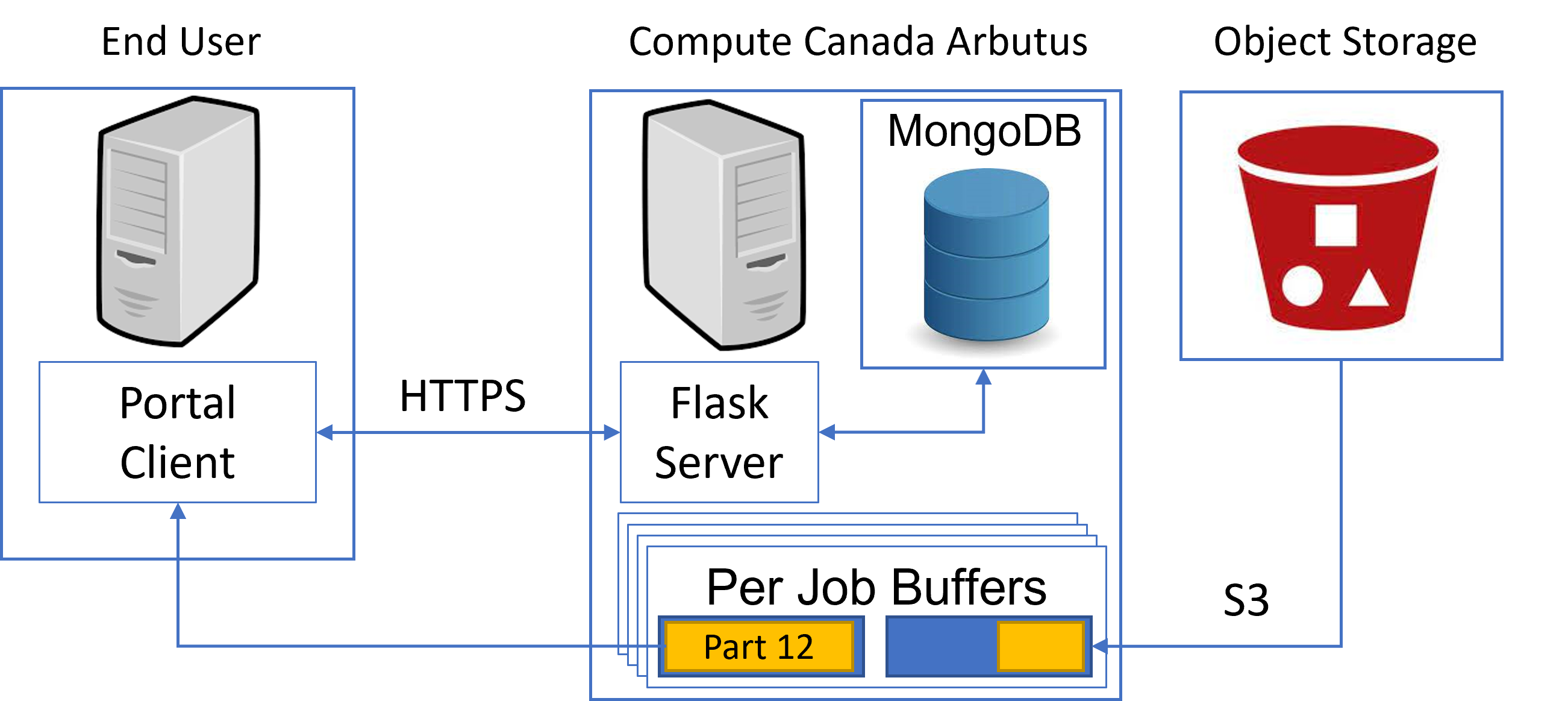
Figure 1: The architecture that provides plant-data to researchers, consisting of the TerraByte Client, the server back-end, and an S3-compatible object storage. In this image the buffer containing part 12 of a dataset is being downloaded by the client, while in parallel the next part of the dataset is being fetched from the object storage by the server into the second buffer.

At the TerraByte project [18] we have the goal to provide labelled plant-data at a similar scale, thus, fuelling the development of better models. For this purpose, we are deploying and developing several systems to collect plant-data in the lab or in the field. Since 2019 we have collected over half a million images in the field and over half a million images in the lab (as of the end of 2021) [19]. The images collected in the lab further contain multiple plants per image, which had been automatically cropped out, resulting in more than 1.5 million images of individual plants. All lab-images are fully labelled, providing information about each plant’s species, planting date, imaging date and more. This data is not only critical for machine learning purposes, but also allows to filter the data by these metadata fields. The species of plants, the age of the plant, and the imaging date, are just three example fields we want to mention here; a full list of the metadata collected is given in Table 1.

Generating and labelling data alone would not be sufficient, however, to sustainably support machine learning research in digital agriculture. As outlined, for example, by Lobet [20], data-collections must have long-term access, storage, and curation. To this end we work together with Compute Canada to host our data in a permanent and unchanging location.

To provide this data to other researchers we are performing several steps: (1) our data is regularly backed up on an object storage system hosted by Compute Canada (CC). (2) The respective metadata is ingested on a database that runs on a server-instance on CC. This instance also hosts the back-end application through which data is delivered from the object storage to the end-user. (3) We have developed a client program, the TerraByte Client (TC), that has been successfully tested on Windows, MacOS, and Unix. This client communicates with the back-end application and can download data to the researcher’s system. The TC can also be used to query the database without having to fully download the dataset in its entirety. Thus, the end-user can quickly check how many images are available under a specified set of filters (for example, how many images of 2-3 week old soybeans are available). Furthermore, samples of such specified datasets can be downloaded within seconds to confirm that these are indeed images that suit the end-user’s goals. By providing these functions, we think a dataset of this size is easier to navigate and data relevant to a specific research question can be found faster. To reduce friction further, we developed a graphical user interface that enables all functionality of the TC; we also deliver the program as an installation-free standalone executable for windows-based machines.

The rest of this paper is structured as follows: In Section II we give an overview on how the TC is operated to obtain data. It follows a short discussion on the client’s performance in Section III. The architecture of the TC and the server’s API is provided in Section IV. Section V offers an outlook on how the TC and the available datasets will evolve.

II Operation

Table 1:

Field	Description
camera & lens	Name of camera used and lens/model used
camera_pose	Coordinates and orientation (pan and tilt) of the camera, when the image was taken
date & time	Date and time when the images was taken
institute & room	Location of the imaging system (more than one imaging system will be in place)
horizontal and vertical dimensions	Dimensions of the image taken
tags	For future use

Metadata fields specific for original (uncropped) images.

Field	Description
plant_id	Unique identifier for each individual plant
label	Common name label for species of plant, e.g. “Soybean”
scientific_name	E.g. “Fallopia convolvulus”
planting_date	Date at which the individual plant was planted
age	Age of the plant when image was taken in days
position_id	An identifier that corresponds to a specific location inside the imagable volume at which the plant was located when the image was taken
x_min, x_max, y_min, y_max	Coordinates of the subimage within the original image

Metadata fields specfic for cropped out single-plant images

(see Figure 3).

The interface of the TC is shown in Figure 2; it consists of several tabs each relating to one class of data and one additional tab providing version-info and useful links. In Figure 2 the active tab is set to EAGL-I Data, which corresponds to images that have been taken in the lab by our robotic imager EAGL-I (see [19]). The tab itself is structured into three sections; via the top two sections the user can define the data they are interested in, whereas the third section contains controls for configuring the tool itself or for interacting with the server-backend.

The filtering options of the first section relate directly to the metadata information that is saved along the image data. Table 1 gives a detailed description of all metadata tracked and we have highlighted fields in boldface that are currently being used by the TC. All filters default to the least restrictive setting and combine in an AND-relation. For example, setting a maximal age of 10 days and a specific plant ID will only give images of that plant ID in which the plant was less than 10 days old. Or stated differently, activating additional filters will generally result in less data fitting the filters. The only exception to this is the multi-select box in which different plant-species can be chosen. Choosing no plant at all in this box deactivates the filter completely, whereas multiple selections will result in every plant that fits into any of the selected species being returned. Thus, within the species-filter we have an OR-relation, while the species-filter itself is combined via AND with the other filters.

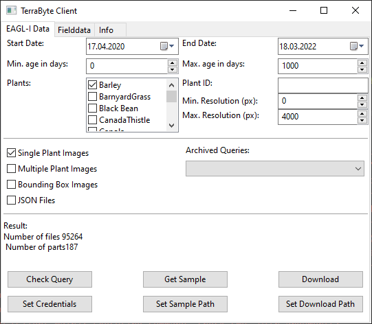
Figure 2: The TerraByte Client user interface currently showing the EAGL-I Data tab, relating to images taken in the lab.

Through the second section in the interface the user can define what types of data they are interested in. This relates to the way the robotic system EAGL-I takes images and we give a brief explanation of that here: EAGL-I moves a camera inside an imageable volume to different positions and from each position one image is taken. Each of those images can contain multiple plants. In a post-processing step each plant is cropped out from the original image separately. This usually leads to more than one cropped out plant image per original image (see Figure 3). We call the cropped out images single plant images and the original images multiple plant images. Further, a copy of the original multiple plant image is created and annotated with the boundaries of the cropped out single plant image. The four selections that can be made in the second section of the interface relate to these three image types and the respective metadata, which is given in a JSON file. Selecting several filetypes will result in all checked filetypes to be returned from the server. Finally, the second section contains a drop-down list that contains pre-compiled datasets. These datasets are permanently stored on the server-backend (in contrast to user-defined datasets that are being pulled from the object storage) and thus can be delivered immediately by the server.

Once the user has defined a dataset through the first two sections, they can query the server in three different ways through the third section of the interface.

• First, the user can check how many files fulfill the specified filter, without committing to any downloads, by using the “Check Query” button. The information returned by the server is displayed in the TC as the number of files and in how many parts these files would be downloaded.

• By using the “Get Sample” button the TC will download a small randomly selected sample per selected filetype. For example, if “Single Plant Images” and “Multiple Plant Images” is selected the TC will download 20 random images of each filetype.

• Finally, the user can download all files resulting from a query by using the “Download” button. This will download all files that fit the specified filters and filetypes.

Three additional buttons are available:

• “Set Credentials”: This opens a dialog in which the user can enter or change their user credentials consisting of username and password. The credentials are saved locally and are reused at future launches of the TC.

• “Set Sample Path”: This allows the user to select in which folder samples should be saved to.

• “Set Download Path”: This allows the user to select in which folder downloads through the “Download”-button will be saved to.

The functionality of the TC when using the “Fielddata”-tab is similar to the one under the “EAGL-I Data”-tab. Future datasets that will be available through the TC client will be accessed through additional tabs, one per dataset, each containing a similar interface.

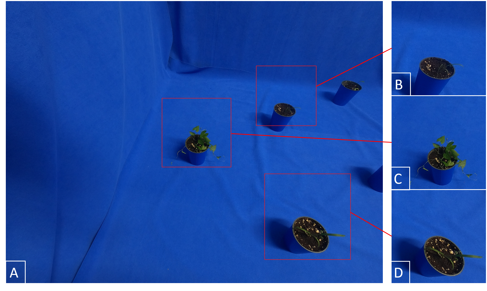
Figure 3: An original image (A) overlayed with the areas that are being cropped out as single-plant images (B-D)

III Performance

The TC’s performance depends on several factors that lie outside of its control:

• The end-systems download-speed and write-speed to drive

• The current load on Compute Canada’s internal network

• The number of clients connected and using the server back-end

To investigate the impact of parallel usage, we tested the system with up to 6 users downloading files at the same time. Only 2 users (user 2 and user 3) shared the same access network. In this test we asked the users to download a predefined dataset of 6193 (542 MB) and measured the time until the data was available on their system. This was compared to the time it took user 1 to download the same files, while no other user is active, which took 130 seconds. We saw that the impact of parallel usage was measurable, yet small, compared to the impact the end-to-end bandwidth between the client’s host and the server has (see Table 2). For example, users 2, 3, and 6 encountered a similar download time independent of whether they downloaded pre-compiled or not pre-compiled datasets. This tells us that the bottleneck in their download speed was not the process of fetching data from the object-storage. Indeed, user-defined (not pre-compiled) datasets impose additional workload on the server that consists of retrieving the data from the object storage and tar-balling the files before sending them to the TC (see the next Section for details). We also saw that downloading pre-compiled datasets is significantly faster if the end-user has enough download bandwidth.

In our testing we further noticed that the performance of the TC and the server-backend fluctuates even if the available bandwidth between client and server remains stable and no other clients are active. We have observed a decrease of download speed up to a factor of 2 in rare instances. When investigating these temporary drops in performances we noticed that the transfer-speed between object storage and server-backend lead to these longer delays. We thus assume that the overall load on Compute Canada’s internal network can impact the system’s overall performance.

Table 2:

	Download Time	Download Speed	Download Time(precompiled)
User 1	316 seconds	1.7 MB/s	36 seconds
User 2	957 seconds	0.56 MB/s	840 seconds
User 3	1,006 seconds	0.53 MB/s	847 seconds
User 4	1096 seconds	0.49 MB/s	49 seconds
User 5	300 seconds	1.8 MB/s	58 seconds
User 6	972 seconds	0.55 MB/s	965 seconds

Performance Test of 6 users downloading 6193 files (542 MB) in parallel

We also performed a long running speed-test for downloading 95K single plant images (9.7 GB) for a single active user, where the data was not precompiled. We repeated that download at several different days to rule out fluctuations stemming from Compute Canada’s internal traffic. The results had been consistent within 1 minute. Similarly we downloaded 20K multiple plant images (34.3 GB) and 15K field data images (105 GB) to compare the download speeds with respect to different filetypes (single plant images are smaller files). The results can be found in Table 3. We can observe that the end-to-end download speed for single plant images lies far below the download speed for the other two categories. The reason for that is the overhead of copying many indiviual small files from the object storage to the server-backend within Compute Canada’s network. For each file we can observe a significant overhead spent on initializing the transfer, resulting in poorer performance.

Table 3:

	Download Time	Download Speed
Single plant images	80 minutes	2 MB/s
Multiple plant images	34 minutes	18 MB/s
Field data images	95 minutes	19 MB/s

Performance test for data from different categories.

IV Architecture

In this section we give a high-level description of the client and server architecture, starting with the client.

IV-A Client Architecture

We focus the discussion on how downloading a user-defined dataset is implemented on the client side. Downloading samples instead or querying the database without starting a download at all are just variations and simplifications of a full download.

The main functionality is defined in $\mathtt{simple\_client.py}$, which provides two key methods: $\mathtt{send\_req}$ and $\mathtt{get\_files}$. The former is a wrapper to send HTTPS POST- and GET-requests to the server’s API. It is used to communicate requests to the database or request a file to be downloaded. In the former case the return of this method is a JSON-formatted object containing the response of the server. When the user wishes to download a dataset $\mathtt{send\_req}$ is used to inform the server about the query parameters. In response the client obtains a unique randomized job-id together with the number of parts the download will consist of. Then the TC main-loop starts the $\mathtt{get\_files}$ method as a subprocess for this job-number and the list of parts.

The $\mathtt{get\_files}$ method repeatedly asks the server if a specific part of a specific job-id is ready to download. To not overload the server with these queries a dynamic backoff period is used, which increases between successive requests. This backoff period resets after a request yields a positive answer from the server. If the server answers that the part is ready for download, $\mathtt{get\_files}$ continues by a direct request to the tar-file via $\mathtt{send\_req}$. The such received data is then unpacked into the download folder on the client side (specified by the user (see Section II). If the server repeatedly answers that the data is not ready, the $\mathtt{get\_files}$ method will eventually reach a maximal number of tries and abandon the download of that part. Once a part is downloaded (or the maximal number of tries exceeded) the main-loop ends that subprocess and moves on to download the next part in a new subprocess. This is repeated until all parts are processed.

Since the main functionality of the client is contained within $\mathtt{simple\_client.py}$ an operation outside the provided graphical user interface is possible. Indeed, the graphical user interface is just a convenient way to construct well-formed HTTPS requests to the server. It is thus possible to skip its usage entirely for the purpose of accessing the server-side API directly within custom code. This allows, for example, to fetch data from the server on-demand from within other methods, such as the iterative training of machine learning models.

IV-B Server Architecture

The server is hosted on Compute Canada on an end-system separate from the data object storage. For communication with the clients the server runs a stack of Flask, MongoDB, and Celery. Flask provides an API over HTTPS, which is also used to deliver the data to the clients. Besides requests that are related to user-management the server handles two types of requests: database queries and download requests.

Database queries from the client are a collection of query parameters which are sanitized and transformed into MongoDB-queries server-side. The such formed MongoDB-query is used to obtain the list of files the user wishes to download in the future. The server also creates a job-id and allocates resources for the upcoming download process. A summary of the file-list is sent back to the client immediately, together with the job-id. Then, using Celery, the server starts a subprocess that downloads the first part of the requested data from the object storage. Once the first part is fully fetched from the object storage those files are tar-balled and are now available for download by the client. Without waiting for the client, the server immediately starts the download of the second part following the same process. However, the third part will only be fetched from the object storage after the first part has been downloaded by the client and the tar-archive has been deleted at the server-instance. The server continues this double-buffered approach, downloading new parts from the object-storage while serving the previously fetched part to the client (see Figure 1). This architecture has two advantages: First, it serves the first parts after a short time to the client thus being a responsive design. Second, we do not have to download the requested dataset in its entirety to the server-instance. In fact, this would be impossible for datasets that exceed the server-instance’s storage (the object storage can host hundreds of TB of data, whereas the server instance has a limited disk space of 5 TB).

V Future Work

We presented the TerraByte Client a tool for downloading user-defined datasets from the TerraByte data-server. We continue our goal to provide labelled plant-data to researchers and industry with the purpose of progressing digital agriculture. To that end, we will extend the client as well as the data-portal along several dimensions:

• More variety in field-data: Future iterations of the data-portal will contain drone data of field images, including test-plots of research facilities and fields of local farmers. Further, we are developing a data-rover that will collect image data in test-plots. More plant-variety in field-data is planned as well.

• Beyond RGB-data: We have several systems that go beyond simple RGB-imaging that are being prepared to ingest data on a large into our database. Amongst these systems are a 3D-scanner for phenotyping purposes, a hyperspectral camera, and a photogrammetry station.

• Additional imagers and plant variety: Next to continuing the operation of EAGL-I, we are setting up additional imaging systems that will image a wider variety of crops and weeds inside our laboratories.

We will further work on improving the overall performance of the client and the server. Specifically, we will increase the end-to-end download speed for user-defined datasets. One options is to have datasets prepared and saved server-side, so that they can be downloaded later at a faster speed. For this purpose, each user will have a limited allocation of disk-space on the server, they can still continue to use the client in the way outlined above as well without space-limitations. Another options is to create archives on the object storage each containing a subset of the data, such that if one file inside a subset is queried it is very likely that other files from that archive are also queried (e.g., one specific day of imaging). Since the data querried usually is highly correlated along such a clustering, transferring an archive from the object storage to the server-backend can yield many relevant files while only paying the transfer overhead once. Indeed, we observed in tests a tranfer speed of more than 150 Mb/s from object storage to the server instance. This would shift the bottleneck of end-to-end transfer to the connectin between the TC and the server instance (for which we observed upload speeds of 20 Mb/s). Further improvements can be achieved by implementing a cache on the level of downloaded archives and a cache on the level of extracted (or copied) files to speed-up follow-up queries.

References

- [1] Ilker Ünal and Mehmet Topakci. Design of a remote-controlled and GPS-guided autonomous robot for precision farming. International Journal of Advanced Robotic Systems, 12:194, 2015.
- [2] Avital Bechar and Clément Vigneault. Agricultural robots for field operations. part 2: Operations and systems. Biosystems Engineering, 153:110–128, 2017.
- [3] Avital Bechar and Clément Vigneault. Agricultural robots for field operations. part 2: Operations and systems. Biosystems Engineering, 153:110–128, 2017.
- [4] Redmond Ramin Shamshiri, C. Weltzien, I. A. Hameed, I. J. Yule, T. E. Grift, S. K. Balasundram, L. Pitonakova, Desa Ahmad, and Girish Chowdhary. Research and development in agricultural robotics: a perspective of digital farming. International Journal of Agricultural and Biological Engineering, 11:1–14, 2018.
- [5] Tom Duckett, Simon Pearson, Simon Blackmore, and Bruce Grieve. Agricultural robotics: The future of robotic agriculture. CoRR, abs/1806.06762, 2018.
- [6] J.E. Relf-Eckstein, Anna T. Ballantyne, and Peter W.B. Phillips. Farming reimagined: a case study of autonomous farm equipment and creating an innovation opportunity space for broadacre smart farming. NJAS - Wageningen Journal of Life Sciences, 90-91:100307, 2019.
- [7] Manlio Bacco, Paolo Barsocchi, Erina Ferro, Alberto Gotta, and Massimiliano Ruggeri. The digitisation of agriculture: a survey of research activities on smart farming. Array, 3-4:100009, 2019.
- [8] Konstantinos G. Liakos, Patrizia Busato, Dimitrios Moshou, Simon Pearson, and Dionysis Bochtis. Machine learning in agriculture: A review. Sensors, 18(8), 2018.
- [9] Kirtan Jha, Aalap Doshi, Poojan Patel, and Manan Shah. A comprehensive review on automation in agriculture using artificial intelligence. Artificial Intelligence in Agriculture, 2:1–12, 2019.
- [10] Bryan C Russell, Antonio Torralba, Kevin P Murphy, and William T Freeman. LabelMe: a database and web-based tool for image annotation. International Journal of Computer Vision, 77:157–173, 2008.
- [11] Michael Buhrmester, Tracy Kwang, and Samuel D Gosling. Amazon’s mechanical turk: A new source of inexpensive, yet high-quality data? Perspectives on Psychological Science, 6:3–5, 2016.
- [12] Christopher J Rapson, Boon-Chong Seet, M Asif Naeem, Jeong Eun Lee, Mahmoud Al-Sarayreh, and Reinhard Klette. Reducing the pain: A novel tool for efficient ground-truth labelling in images. In Proc. IEEE IVCNZ, pages 1–9, 2018.
- [13] Karen Simonyan and Andrew Zisserman. Very deep convolutional networks for large-scale image recognition, 2014.
- [14] Yaniv Taigman, Ming Yang, Marc’Aurelio Ranzato, and Lior Wolf. DeepFace: Closing the gap to human-level performance in face verification. In Proc. IEEE CVPR, 2014.
- [15] Christopher J. Henry, Christopher D. Storie, Muthu Palaniappan, Victor Alhassan, Mallikarjun Swamy, Damilola Aleshinloye, Andrew Curtis, and Daeyoun Kim. Automated LULC map production using deep neural networks. International Journal of Remote Sensing, 40:4416–4440, 2019.
- [16] Kaiming He, Xiangyu Zhang, Shaoqing Ren, and Jian Sun. Delving deep into rectifiers: Surpassing human-level performance on imagenet classification. In Proceedings of the IEEE International Conference on Computer Vision (ICCV), December 2015.
- [17] Olga Russakovsky, Jia Deng, Hao Su, Jonathan Krause, Sanjeev Satheesh, Sean Ma, Zhiheng Huang, Andrej Karpathy, Aditya Khosla, Michael Bernstein, Alexander C. Berg, and Li Fei-Fei. ImageNet large scale visual recognition challenge. International Journal of Computer Vision, 115:211–252, 2015.
- [18] Michael Beck, Christopher Bidinosti, and Christopher Henry. Terrabyte homepage, May 2021c.
- [19] Michael A. Beck, Chen-Yi Liu, Christopher P. Bidinosti, Christopher J. Henry, Cara M. Godee, and Manisha Ajmani. An embedded system for the automated generation of labeled plant images to enable machine learning applications in agriculture. PLOS ONE, 15(12):1–23, 12 2020.
- [20] Guillaume Lobet. Image analysis in plant sciences: Publish then perish. Trends in Plant Science, 22(7):559–566, 2017.