Preprocessing Reward Functions for Interpretability

Abstract

In many real-world applications, the reward function is too complex to be manually specified. In such cases, reward functions must instead be learned from human feedback. Since the learned reward may fail to represent user preferences, it is important to be able to validate the learned reward function prior to deployment. One promising approach is to apply interpretability tools to the reward function to spot potential deviations from the user’s intention. Existing work has applied general-purpose interpretability tools to understand learned reward functions. We propose exploiting the intrinsic structure of reward functions by first preprocessing them into simpler but equivalent reward functions, which are then visualized. We introduce a general framework for such reward preprocessing and propose concrete preprocessing algorithms. Our empirical evaluation shows that preprocessed rewards are often significantly easier to understand than the original reward.

1 Introduction

Reinforcement learning (RL) agents have reached superhuman performance in many tasks, such as games, with clearly defined objectives [23, 3, 26]. However, real-world deployment of RL is often hampered by the difficulty of specifying an appropriate reward function by hand. A variety of methods to learn reward functions have been developed to address this challenge. These algorithms learn from human feedback such as demonstrations [15, 18, 28, 9, 2, 11, 5], preferences [1, 27, 6, 21, 29, 11, 5], or even the initial state of the environment [22].

This gives rise to a new problem: how can we evaluate the learned reward function, and spot potential failure modes before deployment? We could train a policy on the reward model, and then evaluate this policy, such as by humans judging rollouts from the policy. However, this approach has serious drawbacks. Training a policy can be very expensive in complex environments, which makes it hard to quickly compare different learned rewards. It is also brittle: if the trained policy doesn’t perform well, it is unclear whether the fault lies with the reward function or the policy training procedure.

Moreover, we might want to know how well a learned reward transfers to different environment dynamics. Indeed, transfer is a major motivation for learning a reward rather than just directly learning a policy. But it is often challenging to specify the set of dynamics under which we would like the reward to be robust. Even where this is possible, training and evaluating a policy on all such environments is typically infeasible.

To address these problems, prior work introduced the EPIC distance [10] to quantify the difference between two reward functions. When a ground truth reward is available, we can evaluate a learned reward simply by computing its EPIC distance to the ground truth. However, reward learning is most useful precisely when we do not have access to a ground truth reward. In this setting, EPIC may still have some limited utility for comparing and perhaps clustering several learned reward models, but it cannot tell us if any of these learned models are correct.

Michaud et al. [14] instead suggest interpreting reward models to verify they capture user preferences. They find existing interpretability methods such as saliency maps can help understand reward models. However, they also found significant limitations in this approach, concluding that “reward interpretability may need significantly different methods from policy interpretability”.

We believe that significant advances in reward interpretability can be made by taking advantage of the special structure of reward functions. In particular, many different reward functions are equivalent, in the sense that they induce the same optimal policies – no matter the environment dynamics. Given a learned reward model, we can apply transformations that do not change the optimal policy, but simplify the reward function. We can then visualize this simplified reward instead of the original. We call this approach reward preprocessing, as we “preprocess” the reward model prior to visualization.

Our framework for reward preprocessing involves two key components: 1) a class of reward transformations that yield equivalent reward functions in some sense (e.g. by preserving the optimal policy under arbitrary environment dynamics), and 2) an objective that measures how interpretable a given reward function is. We then optimize over the class of transformations using the given objective to find the most interpretable equivalent reward function. A key property of this framework is that the learned reward model is treated as a black box. This means that it may use an arbitrary function approximator and can be learned using any reward learning algorithm and feedback modality.

In summary, our key contributions are: 1) a novel framework that exploits the intrinsic structure of reward functions to increase their interpretability before visualization. 2) Two concrete applications of this framework, using different objectives for interpretability. 3) An empirical evaluation, finding that our methods often significantly improve interpretability.

2 The Reward Preprocessing Framework

Our interpretability method operates on a reward function $r(s,a,s^{\prime})$, where $s$ is the current state, $a$ is the action taken in that state, and $s^{\prime}$ is the next state. Our method only requires the ability to evaluate $r$: there are no restrictions on how $r$ is computed or how it was learned. From $r$, we produce a simpler but equivalent reward function $r^{\prime}$, which we then visualize.

Concrete instantiations of this framework must make two choices. First, they must specify which reward functions are deemed equivalent via an equivalence relation $\sim$. Second, they must provide some measure of “simplicity” or “interpretability”, represented by a cost function $J$. We then seek to find a minimum cost reward function $r^{\prime}$ that is equivalent to $r$:

$$r^{\prime}:=\operatorname*{arg\,min\>}_{\hat{r}\sim r}J(\hat{r}).$$ (1)

In the following, we discuss how to choose the equivalence relation $\sim$ and cost function $J$.

2.1 Equivalence Relation

We would like to treat two rewards as equivalent if they will produce the same behaviour in the intended downstream application. It is known that potential shaping [16] and rescaling by a positive constant never change the ordering of policies. It is therefore safe to treat such rewards as equivalent for most applications.

However, some applications permit a broader notion of equivalence. For example, if the reward model will only ever be used for policy optimization in a specific task, then we can include any transformations that preserve optimal policies in that task. A simple example is $S^{\prime}$-redistribution: moving reward between different successor states, while preserving $\mathbb{E}_{S^{\prime}}r(s,a,S^{\prime})=\mathbb{E}_{S^{\prime}}r^{\prime}(s,a,S^{\prime})$. This will not change the optimal policy, so long as the transition dynamics determining $S^{\prime}$ remain fixed. Skalse et al. [24] characterize a variety of such equivalence classes under varying assumptions.

2.2 Choosing Cost Functions

The cost function $J$ should represent the interpretability of a reward function. Of course, no simple objective can capture the entire concept of interpretability since reward functions may be interpretable for a variety of reasons. For example, sparse rewards are often interpretable, as the user can pay attention only to the few transitions on which the agent receives a non-zero reward. However, a dense reward could still be easy to understand if it has some other simple structure: for example, taking on only two different values depending on which region of the world the agent is in.

Instead of looking for a single cost function that completely characterizes interpretability, we therefore suggest using multiple cost functions, each of which describes some condition that is sufficient but not necessary for interpretability. We can then find an optimal equivalent reward for each of the cost functions and present all of these rewards for the user to choose between. We can also rank the reward functions provided the cost functions are on a comparable scale, presenting lowest-cost rewards first.

Another factor determining the appropriate cost functions is the method used for visualization. For example, a reward function that has sparse output is ideal if we wish to show the user the reward of particular transitions. However, we might prefer sparsity in the features that the reward depends on if using higher-level visualization methods like saliency maps.

3 Methodology

In this section, we describe a few simple concrete instances of our reward preprocessing framework. Despite their simplicity, we find in section 4 that they nonetheless can yield significant improvements. However, these choices are likely far from optimal, and so should be viewed as establishing a lower bound on the benefit obtainable from reward preprocessing.

3.1 Potential Shaping Equivalence Relation

We define two rewards to be equivalent, $r\sim r^{\prime}$, if they are equal up to potential shaping [16]. Specifically, $r\sim r^{\prime}$ if there exists some real-valued state-only function $\Phi$ called a potential for which $r^{\prime}(s,a,s^{\prime})=r(s,a,s^{\prime})+\gamma\Phi(s^{\prime})-\Phi(s)\,$, where $\gamma\in[0,1)$. Potential shaping changes the returns of an episode by only the potential $\Phi(s_{0})$ of the initial state (in the finite horizon case, the potential of terminal states is restricted to be zero). Since the policy does not affect the initial state, the ordering over policies is invariant under potential shaping. This holds for arbitrary transition dynamics and initial state distributions. Therefore, rewards related to each other by potential shaping can be considered equivalent even under transfer to different environment dynamics.

A notable advantage of potential shaping for our purposes is that it is very easy to optimize over the resulting equivalence class. We simply parametrize the potential as a neural network $\Phi_{\theta}(s)$ with parameters $\theta$. Then the optimization problem from eq. 1 becomes

$$\operatorname*{arg\,min\>}_{\theta}J(r^{\prime}_{\theta})\,,\>\text{where}\>r^{\prime}_{\theta}(s,a,s^{\prime})=r(s,a,s^{\prime})+\gamma\Phi_{\theta}(s^{\prime})-\Phi_{\theta}(s).$$ (2)

We optimize eq. 2 using (stochastic) gradient descent. This requires a differentiable cost function $J$, but does not require the reward function $r$ to be differentiable.

Rewards differing by a positive scale factor also produce the same policy ordering. However, since our visualization techniques can handle rewards at a range of scales, we choose to preserve the scale during preprocessing. Accordingly, we do not include rescaled rewards as equivalent.

3.2 Cost Functions

We evaluate two types of cost functions: a sparsity-inducing one based on the $L^{1}$ norm and a smoothness-inducing measure of absolute deviation. In tabular (gridworld) settings, we evaluate these cost functions on a uniform distribution $\mathcal{D}$ over all possible transitions. In continous control environments, we evaluate on transitions sampled from the same distribution $\mathcal{D}$ used for visualization.

Sparse rewards are easy to understand as the user only needs to attend to rewards with non-zero transitions. However, the $L^{0}$ norm is non-differentiable. Moreover, even if the ground-truth reward is sparse, learned reward functions are usually not exactly equivalent to a sparse reward due to the presence of noise. We therefore use two different relaxed notions of sparsity: the $L^{1}$ norm $\left\lvert r\right\rvert$ and the slightly transformed version $\log(1+\left\lvert r\right\rvert)$. In particular, we minimize:

$$J_{\text{sparse}}(r):=\mathbb{E}_{(s,a,s^{\prime})\sim\mathcal{D}}\,f\big{(}r(s,a,s^{\prime})\big{)}\,,$$ (3)

where $\mathcal{D}$ is the distribution over transitions and $f(x)$ is either $\left\lvert x\right\rvert$ or $\log(1+\left\lvert x\right\rvert)$.

An alternative is to minimize the fluctuations between rewards of transitions adjacent in time. This creates a smoothly varying reward signal. The user can then understand the reward by looking at the trend over time. This frees the user from having to attend to the reward at every single transition, similar to sparsity. Again, we use an $L^{1}$ and a logarithmic version of such a smoothness cost:

$$J_{\text{smooth}}(r):=\mathbb{E}_{(s_{t},a_{t},s_{t+1},a_{t+1},s_{t+2})\sim\mathcal{D}}\,f\big{(}r(s_{t},a_{t},s_{t+1})-r(s_{t+1},a_{t+1},s_{t+2})\big{)}\,.$$ (4)

4 Results

We evaluate our methods in two environments: a gridworld, with varying rewards, and the classic mountain car continuous control task [4]. We test our method with a mixture of hand-designed and learned rewards. The hand-designed rewards consist of a simple ground-truth reward, with shaping and/or noise added to challenge the preprocessing method. The learned rewards are trained via either adversarial inverse reinforcement learning [9, AIRL], or via deep reinforcement learning from human preferences [6, DRLHP]. Both methods are trained on synthetic data, consisting of rollouts from an expert policy (AIRL) or preference comparisons induced by the ground-truth reward (DRLHP).

In gridworld experiments, we use a tabular potential and reward model. That is, we learn a separate value $\Phi(s)$ and $r(s,a,s^{\prime})$ for each state and transition. In mountain car, we use small MLPs for the reward model and potentials, except for some cases where a linear potential is sufficient to find a simple equivalent reward. Our code is available at https://github.com/HumanCompatibleAI/reward-preprocessing.

4.1 Simplifying Shaped Rewards

We start by testing our method in a gridworld setting [30]. While unrealistic, gridworlds have the considerable benefit of allowing the entire reward function to be easily visualized. This therefore allows a more thorough evaluation of our method than in other tasks.

In figs. 1 and 2, we visualize gridworld rewards before (leftmost column) and after (middle and right column) our preprocessing methods. In the Goal environment in fig. 1, the reward is simply $1$ on a single goal square in the top right corner and $0$ everywhere else. This is readily understood and our preprocessing largely retains this reward unchanged. However, when we add shaping with the Manhattan distance from the goal (second row), the reward becomes much harder to understand. Our preprocessing, however, is able to simplify this shaped reward to something close to the original sparse objective. Similar results hold for the negative Manhattan distance from the goal (third row) and the particularly confusing random shaping (last row).

In the Path environment in fig. 2, the original reward (top left) prefers a specific path for reaching the goal state. Once again, the shaped versions obscure this, but preprocessing reliably recovers a simple and interpretable reward.

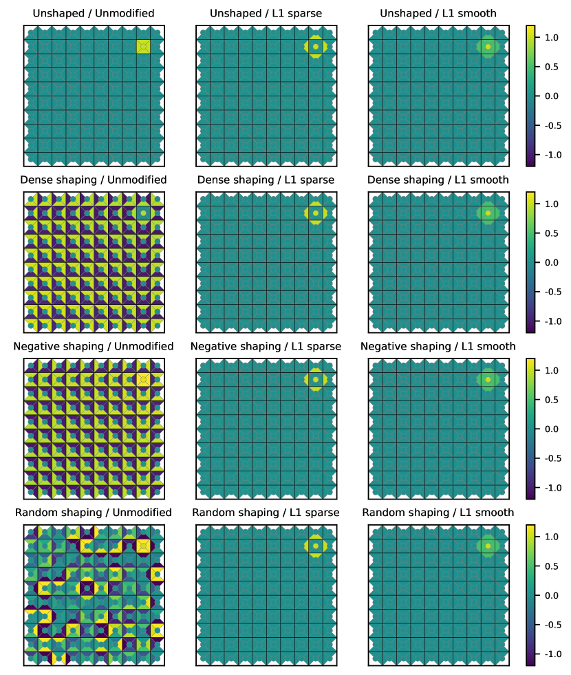
Figure 4: Goal reward preprocessed with $L^{1}$ versions of the sparsity and smoothness cost function. The results are very similar to those in fig. 1. Each heatmap shows the rewards for all possible transitions in a $10\times 10$ gridworld. The circle in the center of each square represents the reward for staying in that state. The four triangles in each square represent the reward of transitions leaving that square in each of the four directions.

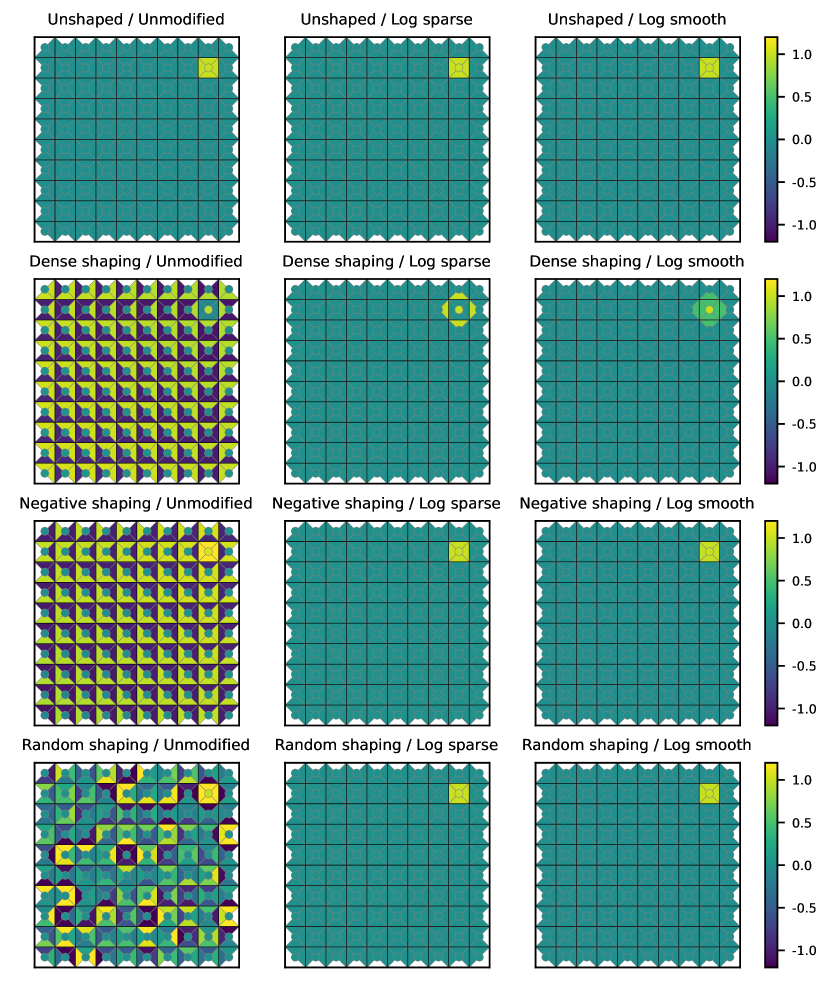
Figure 5: Goal reward preprocessed with logarithmic versions of the sparsity and smoothness cost functions. Again, the results are qualitatively similar to those in fig. 1. Each heatmap shows the rewards for all possible transitions in a $10\times 10$ gridworld. The circle in the center of each square represents the reward for staying in that state. The four triangles in each square represent the reward of transitions leaving that square in each of the four directions.

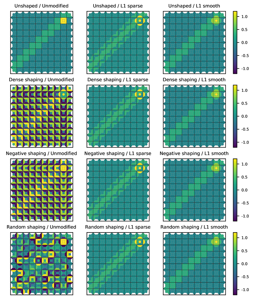
Figure 6: Path reward preprocessed with $L^{1}$ versions of the sparsity and smoothness cost function. The results are very similar to those in fig. 2. Each heatmap shows the rewards for all possible transitions in a $10\times 10$ gridworld. The circle in the center of each square represents the reward for staying in that state. The four triangles in each square represent the reward of transitions leaving that square in each of the four directions.

In these plots, we use the $L^{1}$ version of the sparsity cost and the logarithmic version of the smoothness cost. These work slightly better than the other versions, but the difference is very small. The results for all versions can be found in figs. 4, 5, 6 and 7 in the appendix.

4.2 Understanding Learned Rewards

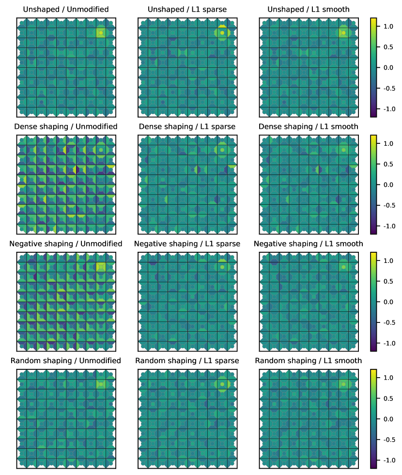
Figure 8: Reward models trained on synthetic data from the Goal reward using preference comparison (leftmost column) and preprocessed versions of these (middle and right). The cost functions used here are the $L^{1}$ version of the sparsity and smoothness cost. Each heatmap shows the rewards for all possible transitions in a $10\times 10$ gridworld. The circle in the center of each square represents the reward for staying in that state. The four triangles in each square represent the reward of transitions leaving that square in each of the four directions.

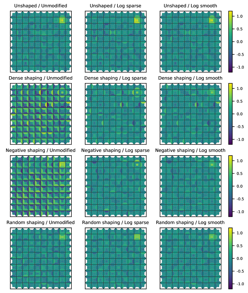
Figure 9: Reward models trained on synthetic data from the Goal reward using preference comparison (leftmost column) and preprocessed versions of these (middle and right). The cost functions used here are the logarithmic version of the sparsity and smoothness cost. Each heatmap shows the rewards for all possible transitions in a $10\times 10$ gridworld. The circle in the center of each square represents the reward for staying in that state. The four triangles in each square represent the reward of transitions leaving that square in each of the four directions.

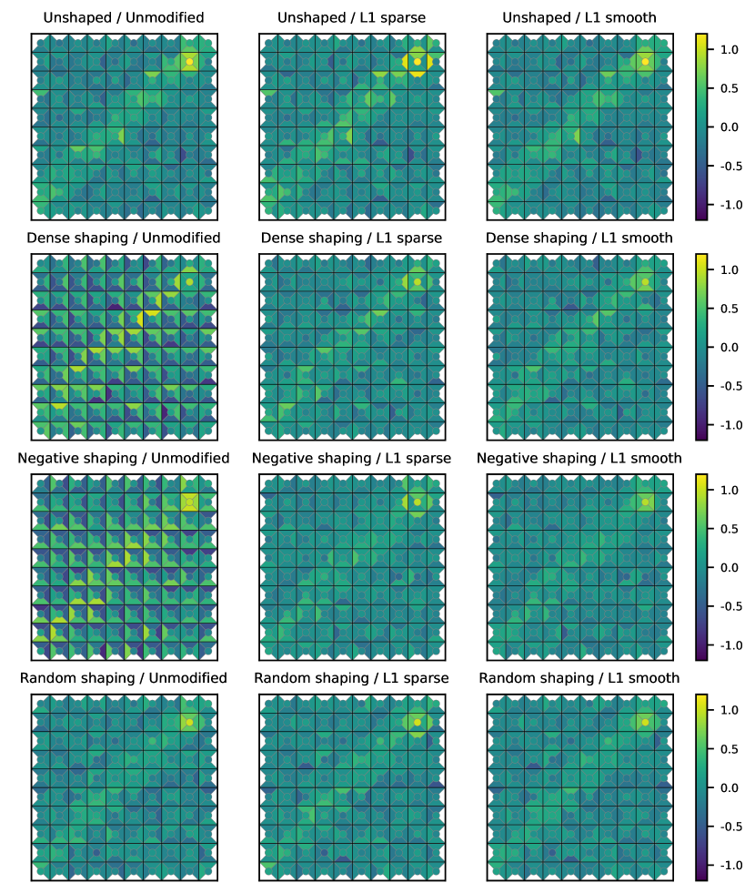
Figure 10: Reward models trained on synthetic data from the Path reward using preference comparison (leftmost column) and preprocessed versions of these (middle and right). The cost functions used here are the $L^{1}$ version of the sparsity and smoothness cost. Each heatmap shows the rewards for all possible transitions in a $10\times 10$ gridworld. The circle in the center of each square represents the reward for staying in that state. The four triangles in each square represent the reward of transitions leaving that square in each of the four directions.

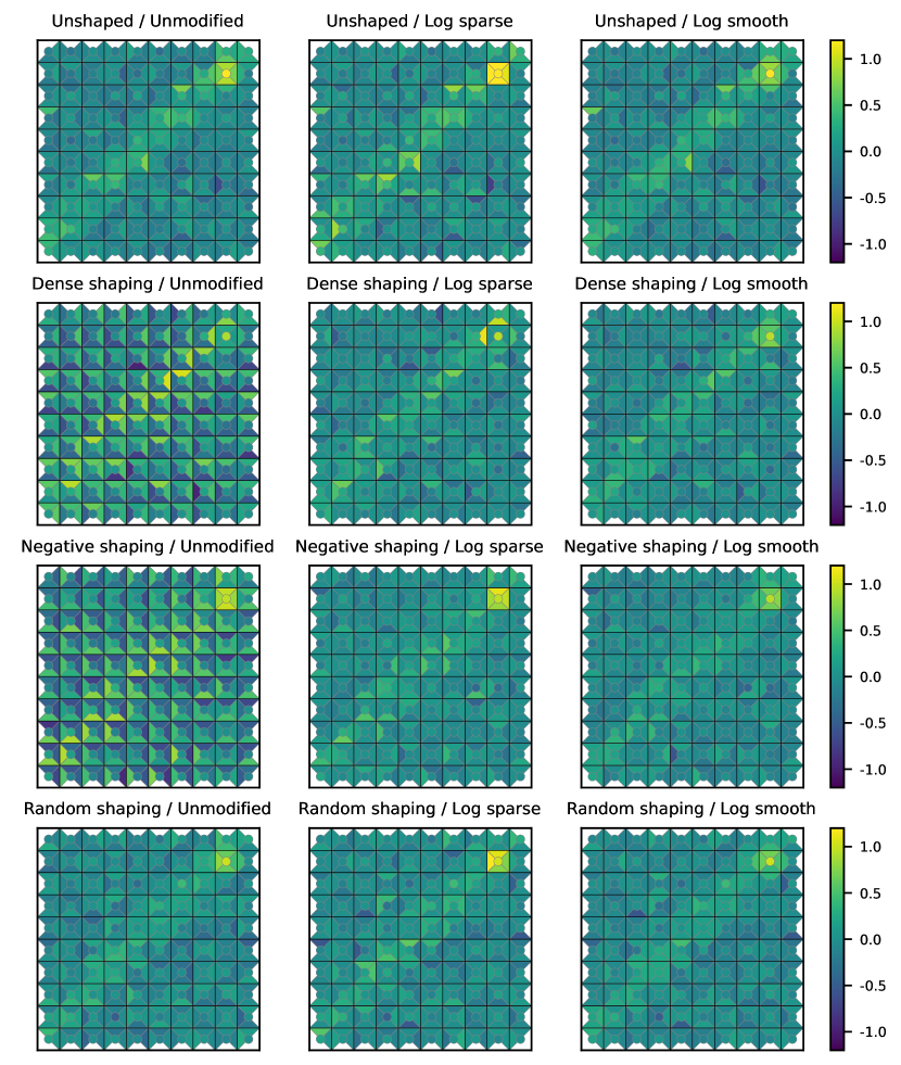
Figure 11: Reward models trained on synthetic data from the Path reward using preference comparison (leftmost column) and preprocessed versions of these (middle and right). The cost functions used here are the logarithmic version of the sparsity and smoothness cost. Each heatmap shows the rewards for all possible transitions in a $10\times 10$ gridworld. The circle in the center of each square represents the reward for staying in that state. The four triangles in each square represent the reward of transitions leaving that square in each of the four directions.

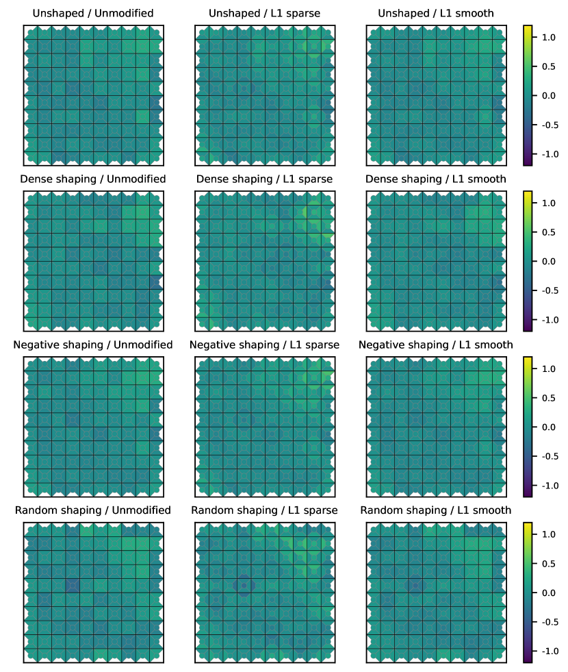
Figure 12: Reward models learned using AIRL from expert demonstrations for the Goal reward (leftmost column) and preprocessed versions of these (middle and right). The cost functions used here are the $L^{1}$ versions of the sparsity and smoothness cost. Each heatmap shows the rewards for all possible transitions in a $10\times 10$ gridworld. The circle in the center of each square represents the reward for staying in that state. The four triangles in each square represent the reward of transitions leaving that square in each of the four directions.

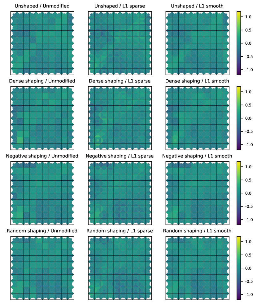
Figure 14: Reward models learned using AIRL from expert demonstrations for the Path reward (leftmost column) and preprocessed versions of these (middle and right). The cost functions used here are the $L^{1}$ versions of the sparsity and smoothness cost. Each heatmap shows the rewards for all possible transitions in a $10\times 10$ gridworld. The circle in the center of each square represents the reward for staying in that state. The four triangles in each square represent the reward of transitions leaving that square in each of the four directions.

In the previous experiment, all the reward functions were exactly equivalent to the simple original reward. By contrast, learned reward models may be noisy or contain systematic errors, and may not be equivalent to any simple reward. To evaluate how our method performs in this more realistic setting, we trained reward models from demonstrations (AIRL) and preference comparisons (DRLHP) on synthetic data in both of the previous Goal and Path environments. The results of applying our preprocessing method are shown in figs. 8, 9, 10, 11, 12, 13, 14 and 15 in the appendix.

For the reward model learned using preference comparisons (DRLHP), even the preprocessed models look very noisy. The goal state does tend to be somewhat more visible in the preprocessed than the unprocessed rewards, but neither are easy to understand. The reward model learned by AIRL differs even more from the ground truth reward, and potential shaping is unable to bridge that gap.

It might be possible to remove more of the noise by using a larger equivalence class than potential shaping. However, expanding the equivalence class might mean the preprocessed reward would no longer induce the same optimal policy as the unmodified reward in some environment dynamics. Indeed, the fact that potential shaping is not sufficient to remove the noise suggests that what DRLHP and AIRL have learned is not just a complex but validly shaped version of the ground truth reward.

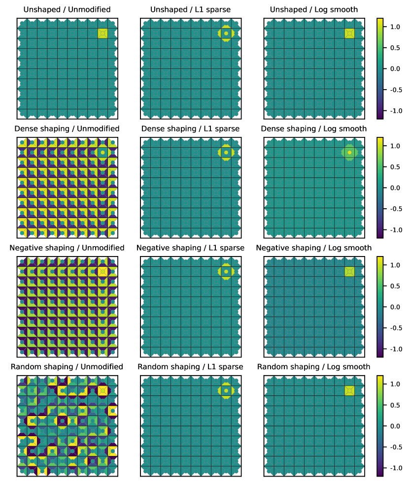
Figure 1: Preprocessing can recover a sparse reward from complex shaping. The original sparse Goal reward is shown in the top-left, with three shaped versions below. These rewards are shown after preprocessing with the sparsity (middle) and smoothness (right) cost functions. The preprocessed rewards are easy to understand, and are similar across a range of shaping. Each heatmap shows the rewards for all possible transitions in a $10\times 10$ gridworld. The circle in the center of each square represents the reward for staying in that state. The four triangles in each square represent the reward of transitions leaving that square in each of the four directions.

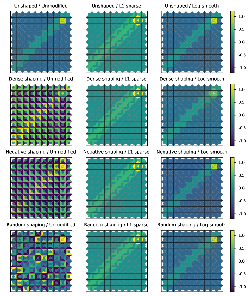
Figure 2: Preprocessing can recover a simpler dense reward from complex shaped rewards. The original Path reward (top-left) incentivizes following a diagonal path to the goal state. The three shaped versions below largely obscure this pattern, but preprocessing is able to recover something similar to the original reward. This is notable as the original reward is not sparse, so still achieves a relatively high cost under the $L^{1}$ norm, but is nonetheless lower cost than the highly complex shaped rewards. Each heatmap shows the rewards for all possible transitions in a $10\times 10$ gridworld. The circle in the center of each square represents the reward for staying in that state. The four triangles in each square represent the reward of transitions leaving that square in each of the four directions.

4.3 Mountain Car

Since the mountain car environment has an infinite number of possible transitions, we cannot plot the rewards of all possible transitions as we did in the gridworld tasks. Instead, we visualize reward functions by plotting the reward signal over time during expert trajectories. Figure 3 visualizes two learned reward models (left) and the reward signal after preprocessing with a log sparse (middle) and log smooth (right) cost function.

The model in the top row was trained using DRLHP on synthetically generated preferences. Specifically, we sampled Boltzmann-rational preferences between trajectory fragments based on the ground truth reward. In the second row, we first learned an optimal state value function for the mountain car environment and then used this to shape the ground truth reward before generating preferences. This simulates human feedback, which may be shaped compared to a sparse ground truth since humans already reward incremental progress [6].

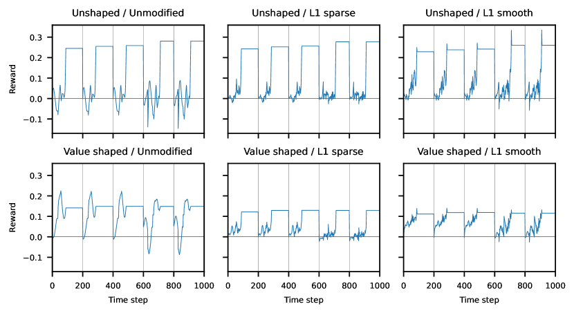
Figure 18: Preprocessing can simplify complex learned reward models for mountain car. The left column shows reward models learned using synthetic preference comparisons based on the ground-truth reward (top), and the ground-truth shaped with an optimal value function (bottom). Preprocessing for sparsity (middle) and smoothness (right) produces simpler and less noisy reward curves, especially in the shaped setting. The results are extremely similar, although perhaps slightly worse, than the logarithmic version used in fig. 3. Each plot shows the reward during a rollout over five episodes (separated by the gray vertical lines).

As in the gridworld setting, both the learned and preprocessed rewards are noisy. However, the preprocessed reward functions are still significantly simpler than the learned models, especially in the shaped case. The sparsity cost function performs better here than the smoothness cost. Figure 3 uses the logarithmic version of both but the $L^{1}$ version in fig. 18 yields almost exactly the same results.

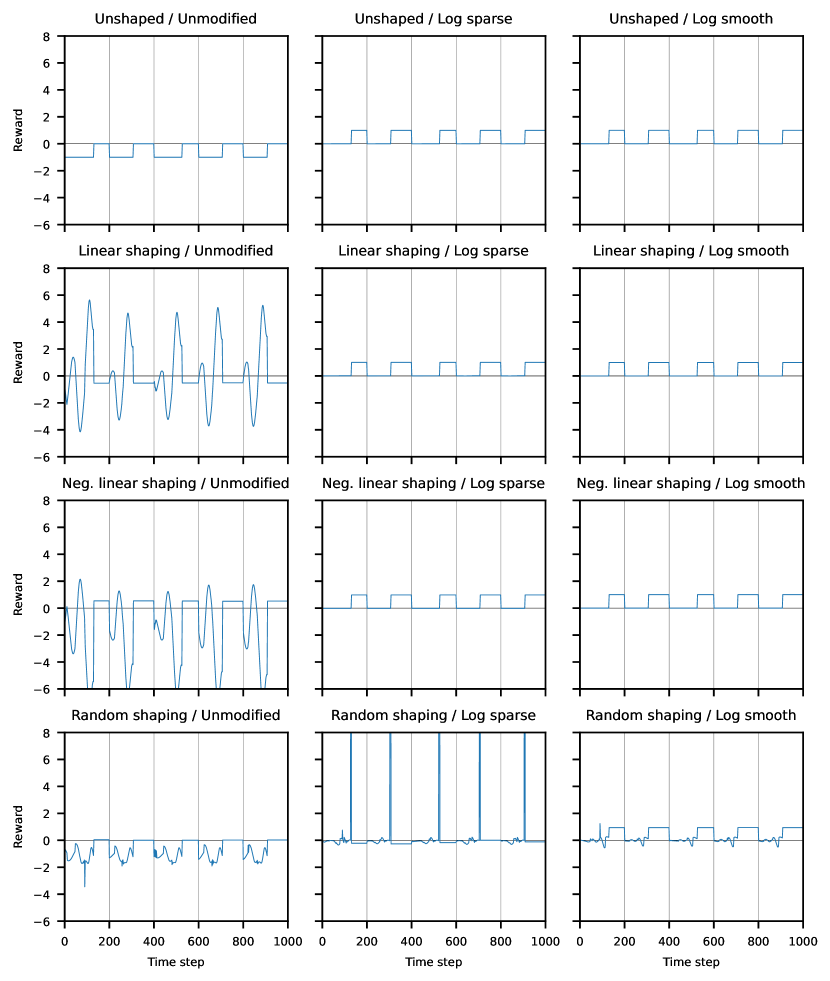
Figure 16: Preprocessing simplifies rewards in the continuous mountain car environment. The top-left shows the ground-truth reward over time, with three shaped versions below. The middle and right column show these rewards after preprocessing using the logarithmic sparsity and smoothness metrics. For the first two (linear) shapings, preprocessing recovers the ground truth reward exactly (up to a constant shift). In the more complex case in the last row, preprocessing still significantly simplifies the reward. See fig. 17 for versions with an $L^{1}$ cost function. Each plot shows the reward during a rollout over five episodes (separated by the gray vertical lines).

Notably, the residual noise after preprocessing in fig. 3 is likely not removable by potential shaping. In particular, we find in figs. 16 and 17 that preprocessing on shaped versions of the ground-truth reward recover simple, noise-free rewards. The residual noise is therefore likely an accurate depiction of errors in the learned reward.

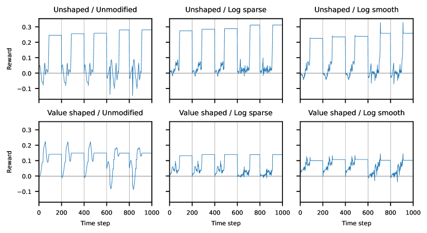
Figure 3: Preprocessing can simplify complex learned reward models for mountain car. The left column shows reward models learned using synthetic preference comparisons based on the ground-truth reward (top), and the ground-truth shaped with an optimal value function (bottom). Preprocessing for sparsity (middle) and smoothness (right) produces simpler and less noisy reward curves, especially in the shaped setting. Each plot shows the reward during a rollout over five episodes (separated by the gray vertical lines).

5 Related Work

Interpreting reward models has recently begun to receive some attention. Russell and Santos [20] apply standard interpretatibility methods from supervised learning to reward functions. Specifically, they use feature importance estimates from a simple fitted global model and from LIME [19] to interpret the reward function.

Globally fitting a simpler model to a reward function has some similarities to our reward preprocessing approach. However, a major difference is that the simple model will usually not be equivalent to the original reward function. In contrast, we learn an equivalent but still simplified reward model. This is possible because we exploit the structure that reward functions naturally have, whereas Russell and Santos [20] only apply preexisting interpretability methods.

Michaud et al. [14] also apply existing interpretability methods to understand reward models. In contrast to Russell and Santos, they work directly with the given reward, without fitting a simpler model. They suggest and combine three different approaches, namely gradient saliency maps, occlusion maps and hand-crafted counterfactual inputs. All of these methods can also be applied to supervised learning more broadly and do not take advantage of the structure of reward functions.

Our reward preprocessing framework is complementary to these methods for interpreting reward functions. We advocate first preprocessing a given reward to select a maximally comprehensible equivalent reward function. The resulting reward function can then be visualized or otherwise interpreted using a range of techniques.

While there is only a handful of work seeking to understand learned reward functions, considerably more work has focused on interpreting policies [17]. One approach is to learn a policy from a class of intrinsically simple functions rather than neural networks [25]. Alternatively, Juozapaitis et al. [12] present a method that explains policy actions by an additive decomposition of $Q$-values. Another promising recent direction is using causal models to explain policy behavior [13, 8].

Devidze et al. [7] approach interpretability of reward functions from a different angle: rather than interpreting a complex learned reward function, they aim to design a reward function that trades off between interpretability (operationalized as sparsity) and ease of policy optimization.

6 Limitations and Future Work

One limitation of our approach is that while potential shaping does not change the optimal policy, it can make the policy optimization problem easier or harder. Consequently, the policy learned by an RL algorithm might well differ between the unmodified learned reward and the theoretically “equivalent” reward used for visualization. This issue is most significant in environments where policy optimization can be challenging. Reasoning about how shaping affects RL algorithm performance is challenging, so this is only a significant factor when the tool is being used by trained practitioners.

The above limitation is a way in which potential shaping can be too big an equivalence class. However, there is also a sense in which it is too small. In practice, we do not usually care about a reward function transferring to all possible transition dynamics. If it is known the transition dynamics satisfy certain invariants, then we may be able to use a larger equivalence class while still guaranteeing optimal policy preservation.

In addition to modifying the equivalence class, there are also numerous alternative cost functions that could be employed. In particular, the cost functions we suggest are targeted at the visualizations we use in this paper. Other visualizations might benefit from different cost functions. However, it seems likely that the basic concepts of sparsity and smoothness will be useful in many settings. For example, visualizations using gradient saliency maps might benefit from maximizing the sparsity of the gradients, rather than of the rewards themselves.

7 Conclusion

We have introduced a novel framework to preprocess reward functions prior to visualization. Our empirical results demonstrate this methodology can recover simple reward functions from shaped versions of ground-truth rewards. Moreover, our method can substantially simplify even noisy learned reward models. However, some low-quality learned reward models are still difficult to understand even with our method, suggesting that reward learning algorithms often converge to models significantly different from the user’s intended preferences.

Appendix A Appendix

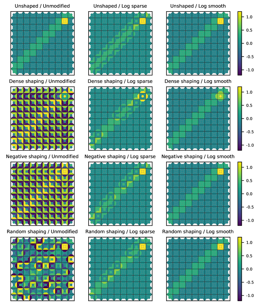
Figure 7: Path reward preprocessed with logarithmic versions of the sparsity and smoothness cost functions. Compared to the $L^{1}$ sparse cost function in fig. 6, the log sparse cost recovers a slightly less symmetric but still significantly simplified reward. Each heatmap shows the rewards for all possible transitions in a $10\times 10$ gridworld. The circle in the center of each square represents the reward for staying in that state. The four triangles in each square represent the reward of transitions leaving that square in each of the four directions.

Figure 13: Reward models learned using AIRL from expert demonstrations for the Goal reward (leftmost column) and preprocessed versions of these (middle and right). The cost functions used here are the logarithmic versions of the sparsity and smoothness cost. Each heatmap shows the rewards for all possible transitions in a $10\times 10$ gridworld. The circle in the center of each square represents the reward for staying in that state. The four triangles in each square represent the reward of transitions leaving that square in each of the four directions.

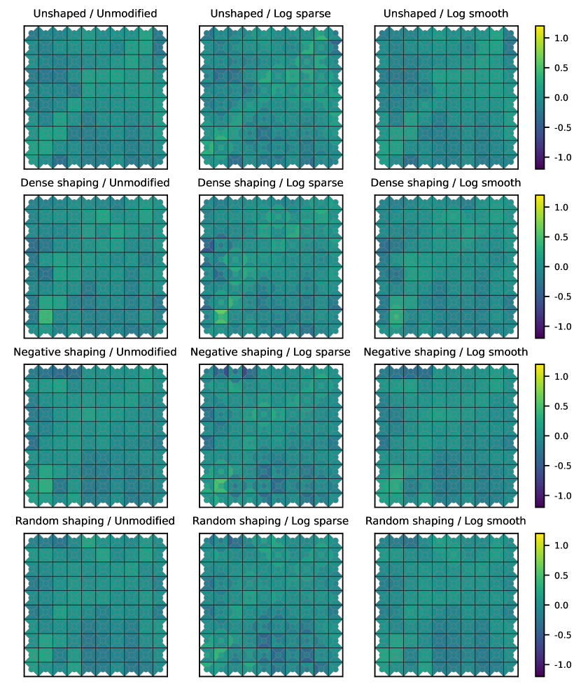
Figure 15: Reward models learned using AIRL from expert demonstrations for the Path reward (leftmost column) and preprocessed versions of these (middle and right). The cost functions used here are the logarithmic versions of the sparsity and smoothness cost. Each heatmap shows the rewards for all possible transitions in a $10\times 10$ gridworld. The circle in the center of each square represents the reward for staying in that state. The four triangles in each square represent the reward of transitions leaving that square in each of the four directions.

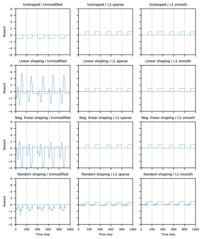
Figure 17: The top-left shows the ground-truth reward in mountain car over time, with three shaped versions below. The middle and right column show these rewards after preprocessing using the $L^{1}$ sparsity and smoothness metrics. This works reasonably well for these simple shaped rewards, although in the more complex last row these cost functions appear to perform less well than the logarithmic version in fig. 16. Each plot shows the reward during a rollout over five episodes (separated by the gray vertical lines).

References

- Akrour et al. [2011] Riad Akrour, Marc Schoenauer, and Michele Sebag. Preference-based policy learning. In Machine Learning and Knowledge Discovery in Databases, 2011.
- Bahdanau et al. [2019] Dzmitry Bahdanau, Felix Hill, Jan Leike, Edward Hughes, Arian Hosseini, Pushmeet Kohli, and Edward Grefenstette. Learning to understand goal specifications by modelling reward. In ICLR, 2019.
- Berner et al. [2019] Christopher Berner, Greg Brockman, Brooke Chan, Vicki Cheung, Przemysław Dębiak, Christy Dennison, David Farhi, Quirin Fischer, Shariq Hashme, Chris Hesse, Rafal Józefowicz, Scott Gray, Catherine Olsson, Jakub Pachocki, Michael Petrov, Henrique P. d. O. Pinto, Jonathan Raiman, Tim Salimans, Jeremy Schlatter, Jonas Schneider, Szymon Sidor, Ilya Sutskever, Jie Tang, Filip Wolski, and Susan Zhang. Dota 2 with large scale deep reinforcement learning. arXiv: 1912.06680 [cs.LG], 2019.
- Boyan and Moore [1995] Justin Boyan and Andrew W Moore. Generalization in reinforcement learning: Safely approximating the value function. In NIPS, pages 369–376, 1995.
- Brown et al. [2019] Daniel S. Brown, Wonjoon Goo, Prabhat Nagarajan, and Scott Niekum. Extrapolating beyond suboptimal demonstrations via inverse reinforcement learning from observations. In ICML, 2019.
- Christiano et al. [2017] Paul F Christiano, Jan Leike, Tom Brown, Miljan Martic, Shane Legg, and Dario Amodei. Deep reinforcement learning from human preferences. In NeurIPS, pages 4299–4307, 2017.
- Devidze et al. [2021] Rati Devidze, Goran Radanovic, Parameswaran Kamalaruban, and Adish Singla. Explicable reward design for reinforcement learning agents. In NeurIPS, 2021.
- Déletang et al. [2021] Grégoire Déletang, Jordi Grau-Moya, Miljan Martic, Tim Genewein, Tom McGrath, Vladimir Mikulik, Markus Kunesch, Shane Legg, and Pedro A. Ortega. Causal analysis of agent behavior for AI safety. arXiv: 2103.03938 [cs.AI], 2021.
- Fu et al. [2018] Justin Fu, Katie Luo, and Sergey Levine. Learning robust rewards with adversarial inverse reinforcement learning. In ICLR, 2018.
- Gleave et al. [2021] Adam Gleave, Michael Dennis, Shane Legg, Stuart Russell, and Jan Leike. Quantifying differences in reward functions. In ICLR, 2021.
- Ibarz et al. [2018] Borja Ibarz, Jan Leike, Tobias Pohlen, Geoffrey Irving, Shane Legg, and Dario Amodei. Reward learning from human preferences and demonstrations in Atari. In NeurIPS, 2018.
- Juozapaitis et al. [2019] Z. Juozapaitis, A. Koul, A. Fern, M. Erwig, and F. Doshi-Velez. Explainable reinforcement learning via reward decomposition. In IJCAI Workshop on Explainable Artificial Intelligence, 2019.
- Madumal et al. [2020] Prashan Madumal, Tim Miller, Liz Sonenberg, and Frank Vetere. Explainable reinforcement learning through a causal lens. In AAAI, 2020.
- Michaud et al. [2020] Eric J. Michaud, Adam Gleave, and Stuart Russell. Understanding learned reward functions. NeurIPS Deep RL workshop, 2020.
- Ng and Russell [2000] Andrew Y. Ng and Stuart Russell. Algorithms for inverse reinforcement learning. In ICML, 2000.
- Ng et al. [1999] Andrew Y. Ng, Daishi Harada, and Stuart Russell. Policy invariance under reward transformations: Theory and application to reward shaping. In ICML, 1999.
- Puiutta and Veith [2020] Erika Puiutta and Eric M. S. P. Veith. Explainable reinforcement learning: A survey. In Machine Learning and Knowledge Extraction, 2020.
- Ramachandran and Amir [2007] Deepak Ramachandran and Eyal Amir. Bayesian inverse reinforcement learning. In IJCAI, 2007.
- Ribeiro et al. [2016] Marco Tulio Ribeiro, Sameer Singh, and Carlos Guestrin. "Why should I trust you?": Explaining the predictions of any classifier. In ACM SIGKDD, 2016.
- Russell and Santos [2019] Jacob Russell and Eugene Santos. Explaining reward functions in markov decision processes. In International Florida Artificial Intelligence Research Society Conference, 2019.
- Sadigh et al. [2017] Dorsa Sadigh, Anca D. Dragan, S. Shankar Sastry, and Sanjit A. Seshia. Active preference-based learning of reward functions. In RSS, July 2017.
- Shah et al. [2018] Rohin Shah, Dmitrii Krasheninnikov, Jordan Alexander, Pieter Abbeel, and Anca Dragan. Preferences implicit in the state of the world. In ICLR, 2018.
- Silver et al. [2016] David Silver, Aja Huang, Chris J. Maddison, Arthur Guez, Laurent Sifre, George van den Driessche, Julian Schrittwieser, Ioannis Antonoglou, Veda Panneershelvam, Marc Lanctot, Sander Dieleman, Dominik Grewe, John Nham, Nal Kalchbrenner, Ilya Sutskever, Timothy Lillicrap, Madeleine Leach, Koray Kavukcuoglu, Thore Graepel, and Demis Hassabis. Mastering the game of Go with deep neural networks and tree search. Nature, 529(7587):484–489, 2016.
- Skalse et al. [2022] Joar Skalse, Matthew Farrugia-Roberts, Stuart Russell, Alessandro Abate, and Adam Gleave. Invariance in policy optimisation and partial identifiability in reward learning, 2022.
- Verma et al. [2018] Abhinav Verma, Vijayaraghavan Murali, Rishabh Singh, Pushmeet Kohli, and Swarat Chaudhuri. Programmatically interpretable reinforcement learning. In ICML, 2018.
- Vinyals et al. [2019] Oriol Vinyals, Igor Babuschkin, Wojciech M. Czarnecki, Michaël Mathieu, Andrew Dudzik, Junyoung Chung, David H. Choi, Richard Powell, Timo Ewalds, Petko Georgiev, Junhyuk Oh, Dan Horgan, Manuel Kroiss, Ivo Danihelka, Aja Huang, Laurent Sifre, Trevor Cai, John P. Agapiou, Max Jaderberg, Alexander S. Vezhnevets, Rémi Leblond, Tobias Pohlen, Valentin Dalibard, David Budden, Yury Sulsky, James Molloy, Tom L. Paine, Caglar Gulcehre, Ziyu Wang, Tobias Pfaff, Yuhuai Wu, Roman Ring, Dani Yogatama, Dario Wünsch, Katrina McKinney, Oliver Smith, Tom Schaul, Timothy Lillicrap, Koray Kavukcuoglu, Demis Hassabis, Chris Apps, and David Silver. Grandmaster level in StarCraft II using multi-agent reinforcement learning. Nature, 575(7782):350–354, 2019.
- Wilson et al. [2012] Aaron Wilson, Alan Fern, and Prasad Tadepalli. A Bayesian approach for policy learning from trajectory preference queries. In NeurIPS, 2012.
- Ziebart et al. [2008] Brian D. Ziebart, Andrew Maas, J. Andrew Bagnell, and Anind K. Dey. Maximum entropy inverse reinforcement learning. In AAAI, 2008.
- Ziegler et al. [2019] Daniel M. Ziegler, Nisan Stiennon, Jeffrey Wu, Tom B. Brown, Alec Radford, Dario Amodei, Paul Christiano, and Geoffrey Irving. Fine-tuning language models from human preferences. arXiv: 1909.08593v2 [cs.CL], 2019.
- Zuo [2018] Xingdong Zuo. mazelab: A customizable framework to create maze and gridworld environments. https://github.com/zuoxingdong/mazelab, 2018.