$\cos 2\phi_{t}$ azimuthal asymmetry in back-to-back $J/\psi$ -jet production in $e\leavevmode\nobreak\ p\rightarrow e\leavevmode\nobreak\ J/\psi\leavevmode\nobreak\ Jet\leavevmode\nobreak\ X$  at the EIC

Abstract

In this article, we investigate the $\cos 2\phi_{t}$ azimuthal asymmetry in $e\leavevmode\nobreak\ p\rightarrow e\leavevmode\nobreak\ J/\psi\leavevmode\nobreak\ Jet\leavevmode\nobreak\ X$, where the $J/\psi$-jet pair is almost back-to-back in the transverse plane, within the framework of the generalized parton model(GPM). We use non-relativistic QCD(NRQCD) to calculate the $J/\psi$ production amplitude and incorporate both color singlet(CS) and color octet(CO) contributions to the asymmetry. We estimate the asymmetry using different parameterizations of the gluon TMDs in the kinematics that can be accessed at the future electron-ion collider (EIC) and also investigate the impact of transverse momentum dependent (TMD) evolution on the asymmetry. We present the contributions coming from different states to the asymmetry in NRQCD.

I Introduction

Transverse momentum dependent parton distributions (TMDs)Mulders and Tangerman (1996); Boer and Mulders (1998); Boer et al. (2000); Anselmino et al. (1999, 1995); Barone et al. (2002) give a tomographic picture of the nucleon in terms of quarks and gluons in momentum space. TMDs play an important role in processes where two scales are involved; for example, in semi-inclusive deep inelastic scattering (SIDIS) where apart from the photon virtuality, one measures the transverse momentum of the outgoing particle, or Drell-Yan process where the transverse momentum of the outgoing lepton-pair provide the second scale. For such processes, one can apply the generalized factorization involving TMDs. However, the TMD factorization has not been proven for all processes. In the kinematical limit when the collinear factorization becomes valid, the result based on TMD factorization should be matched with that obtained using collinear factorization in the same process, with the inclusion of soft factors in the TMD framework Collins (2011); Echevarria et al. (2012); Echevarría et al. (2013); Echevarria (2019); Bacchetta et al. (2008); Fleming et al. (2020). To ensure gauge invariance, the TMDs include gauge links or Wilson lines, which comes due to initial or final state interactions Collins (2002); Ji and Yuan (2002); Belitsky et al. (2003); Boer et al. (2003). These introduce process dependence in them. Recent results from RHIC are in favour of the theoretical prediction of a sign change of the Sivers function observed in SIDIS and DY processes, respectivelyAnselmino et al. (2017). More data is needed to have a firm understanding of the process dependence of the TMDs. Gluon TMDs Mulders and Rodrigues (2001) till now are far less investigated than the quark TMDs. The positivity bound gives a constraint on them Mulders and Rodrigues (2001). Recently, there is an extraction of unpolarized gluon TMDs from LHCb data Lansberg et al. (2018). Gauge invariance of the gluon TMDs requires the inclusion of two gauge links in the definition, which makes the process dependence more involved than the quark TMDs Buffing et al. (2013). The most common are one past and one future pointing gauge links, $[+-]$ or $[-+]$ (f-type) and both past or both future pointing, $[--]$ or $[++]$ (d-type). The operator structures of these two types of gluon TMDs are different Buffing et al. (2013). In the literature on small-$x$ physics, these two gluon TMDs are called Weiszacker-Williams (WW) Kovchegov and Mueller (1998); McLerran and Venugopalan (1999) type and dipole Dominguez et al. (2012) type, respectively. These contribute in different processes.

In an unpolarized proton, there is a nonzero probability of finding linearly polarized gluons. The linearly polarized gluon distributions were introduced in Mulders and Rodrigues (2001), and first investigated in a model in Meissner et al. (2007). Recently these have attracted quite a lot of attention, although till now they have not been extracted using data. Linearly polarized gluon distributions can be probed in $ep$ and $pp$ collisions Marquet et al. (2018); Pisano et al. (2013); Boer et al. (2009); Efremov et al. (2018a, b); Lansberg et al. (2017); Dumitru et al. (2019); Sun et al. (2011); Boer et al. (2013, 2012); Echevarria et al. (2015); Boer and Pisano (2012a); Mukherjee and Rajesh (2017a); Mukherjee and Rajesh (2016). These give an azimuthal asymmetry of the form $\cos\leavevmode\nobreak\ 2\phi_{t}$Pisano et al. (2013); also, they affect the transverse momentum distribution of the outgoing particle. Depending on the gauge links, the linearly polarized gluon distribution can be WW or dipole type. These are time reversal even (T-even) objects. In $pp$ scattering processes, the initial and final state interactions often affect the TMD factorization; the asymmetries and cross sections also involve both f-type and d-type gluon TMDs, and disentangling the two is difficult from the observables. The gauge link structure is simpler in $ep$ scattering processes Rajesh et al. (2021), and the upcoming electron-ion collider (EIC) at Brookhaven National Lab will play an important role in probing the gluon TMDs, including the linearly polarized gluon TMD over a wide kinematical region.

$\cos\leavevmode\nobreak\ 2\phi_{t}$ asymmetry in $J/\psi$ production in unpolarized $ep$ collision has been shown to be a useful observable to probe the linearly polarized gluon TMD. Contribution to the asymmetry comes already at the leading order (LO) through the virtual photon-gluon fusion process Mukherjee and Rajesh (2017b); this contributes at $z=1$, where $z$ is the fraction of the energy of the photon carried by the $J/\psi$ in the rest frame of the proton. In the kinematical region $z<1$ Kishore and Mukherjee (2019) one has to incorporate higher order Feynman diagrams. In this process, the $J/\psi$ produced needs to be detected in the forward region, or with its transverse momentum $\mathrm{p}_{T}$ not so large; otherwise TMD factorization is not expected to hold. In this work, we investigate the $\cos 2\phi_{t}$ asymmetry in a slightly different process, namely when a $J/\psi$ and a jet are observed almost back-to-back in $ep$ collision. Only the WW type gluon TMDs contribute in this process D’Alesio et al. (2019). Here the $J/\psi$ produced can have large transverse momentum, as the soft scale required for the TMD factorization is provided by the total transverse momentum of the $J/\psi$-jet pair, which is smaller than their invariant mass as they are almost back-to-back Kishore et al. (2020). In fact, by varying the invariant mass of the pair, one can also probe the TMDs over a wide range of scales and investigate the effect of TMD evolution on the asymmetry. In D’Alesio et al. (2019), the upper bound of the $\cos\leavevmode\nobreak\ 2\phi_{t}$ asymmetry was investigated in this process, as well as the asymmetry in the small-$x$ region. Here we present a calculation of the asymmetry using some recent parameterization of the gluon TMDs and also investigate the effect of TMD evolution.

A widely used approach to calculate the amplitude of $J/\psi$ production is based on an effective field theory called non-relativistic QCD (NRQCD) Hägler et al. (2001); Yuan and Chao (2001); Yuan (2008). Here, one assumes that the amplitude for $J/\psi$ production process can be factorized into a hard part where the $c\bar{c}$ pair is produced perturbatively, and a soft part where the heavy quark pair hadronizes to form a $J/\psi$. The hadronization process is encoded in the long distance matrix elements (LDMEs) Bodwin et al. (1995); which are usually extracted using the data. The cross-section is expressed as a double expansion in terms of the strong coupling $\alpha_{s}$ as well as the velocity parameter associated with the heavy quark $v$Boer et al. (2021); Lepage et al. (1992); in the limit $v\ll 1$. For charmonium $v\approx 0.3$. The heavy quark pair in the hard process is produced in different states denoted by ${}^{2s+1}L_{J}^{(c)}$ where $s$ denotes the spin of the pair (singlet or triplet), $L$ is the orbital angular momentum, $J$ is the total angular momentum and $(c)$ denotes the color configuration, which can be singlet or octet. The heavy quark pair produced in the hard process emits soft gluons to evolve into $J/\psi$. For the $S$-wave contribution, the dominant term in the limit $v\approx 0$ gives the result of the color singlet model (CSM)Berger and Jones (1981); Baier and Rückl (1983), where the heavy quark pair in the hard process is assumed to be produced with the same quantum numbers as the $J/\psi$, and in the color singlet state. In our work, we include both color singlet (CS) and color octet (CO) contributions.

The paper is arranged as follows: In section II, we present the TMD formalism adopted. In Section III, we investigate the effect of the TMD evolution on the asymmetries. In sections IV and V, we present two recent parameterizations of the gluon TMDs, based on the spectator model and a Gaussian parameterization, respectively. Numerical results are presented in section VI. The conclusion is discussed in section VII.

II Formalism

We consider a semi-inclusive electroproduction of a $J/\psi$ and a jet,

$$e^{-}(l)+p(\mathrm{P})\to e^{-}(l^{\prime})+J/\psi(\mathrm{P}_{\psi})+Jet(\mathrm{P}_{j})+X,$$

where the four-momentum of the particles are given in their corresponding round brackets. Here, both the incoming electron beam and the target proton are unpolarized with their respective momenta $l$ and $P$. The kinematics of the process can be described in the following variables

$$Q^{2}=-q^{2},\leavevmode\nobreak\ \leavevmode\nobreak\ \leavevmode\nobreak\ \leavevmode\nobreak\ \leavevmode\nobreak\ \leavevmode\nobreak\ s=(P+l)^{2},\leavevmode\nobreak\ \leavevmode\nobreak\ \leavevmode\nobreak\ \leavevmode\nobreak\ \leavevmode\nobreak\ \leavevmode\nobreak\ \leavevmode\nobreak\ \leavevmode\nobreak\ \leavevmode\nobreak\ W^{2}=(P+q)^{2},$$ (1)

$$x_{B}=\frac{Q^{2}}{2P\cdot q},\leavevmode\nobreak\ \leavevmode\nobreak\ \leavevmode\nobreak\ \leavevmode\nobreak\ \leavevmode\nobreak\ \leavevmode\nobreak\ \leavevmode\nobreak\ \leavevmode\nobreak\ \leavevmode\nobreak\ \leavevmode\nobreak\ y=\frac{P\cdot q}{P\cdot l},\leavevmode\nobreak\ \leavevmode\nobreak\ \leavevmode\nobreak\ \leavevmode\nobreak\ \leavevmode\nobreak\ \leavevmode\nobreak\ \leavevmode\nobreak\ \leavevmode\nobreak\ \leavevmode\nobreak\ \leavevmode\nobreak\ \leavevmode\nobreak\ \leavevmode\nobreak\ \leavevmode\nobreak\ z=\frac{P\cdot\mathrm{P}_{\psi}}{P\cdot q}.$$ (2)

The virtuality of the scattering photon is given by $Q^{2}$, $s$ is the square of the electron-proton center of mass energy whereas, $W$ is the invariant mass of photon-proton system. $x_{B}$ is the Bjorken-$x$ variable, $y$ is the inelasticity variable that gives the fraction of the energy of the electron taken by the scattering virtual photon and the variable $z$ defines the fraction of energy of the photon carried by the outgoing $J/\psi$ particle in proton rest frame. We consider virtual photon-proton center of mass frame where they move along $+z$ and $-z$ directions, respectively. To define the kinematics, we use the light-cone coordinate system. We use two light-like vectors, one of which is chosen to be in the direction of the proton momentum, $P=n_{-}$ and the other $n=n_{+}$, such that $P\cdot n=1$ and $n_{-}^{2}=n_{+}^{2}=0$. In terms of these vectors, the momenta of the particles involved in the process can be written as follows;
Momenta of the initial proton and virtual photon can be expressed as

$$P^{\mu} =n_{-}^{\mu}+\frac{M_{p}^{2}}{2}n_{+}^{\mu}\approx n_{-}^{\mu},$$ (3)

$$q^{\mu} =-x_{B}n_{-}^{\mu}+\frac{Q^{2}}{2x_{B}}n_{+}^{\mu}\approx-x_{B}P^{\mu}+(P\cdot q)n_{+}^{\mu},$$ (4)

where $M_{p}$ is proton mass and $Q^{2}=x_{B}ys$. The expressions for the incoming and outgoing lepton momenta can be written in terms of light cone coordinates using the inelasticity variable $y$ as,

$$l^{\mu} =\frac{(1-y)x_{B}}{y}P^{\mu}+\frac{(P\cdot q)}{y}n^{\mu}+\frac{\sqrt{1-y}}{y}Q\hat{l}_{\perp}^{\mu},$$ (5)

$$l^{\prime\mu} =l^{\mu}-q^{\mu}.$$ (6)

At the partonic level process, $J/\psi$ can either be produced through the gluonic channel: $g+\gamma^{\star}\to J/\psi+g$ or through the quark (anti-quark) channel: $q(\bar{q})+\gamma^{\star}\to J/\psi+q(\bar{q})$. However, in the small-$x$ region, the gluonic channel dominates over the quark (anti-quark) channel D’Alesio et al. (2019). Hence, we have considered the contribution from the gluonic channel only in the following estimate of the asymmetry. The above processes contribute at the next-to-leading (NLO) order in $\alpha_{s}$ and in the kinematic region $z<1$. The outgoing energetic gluons produced in this process gives the jet. Now, we can express the momentum of the initial gluon, $p_{g}$, the final $J/\psi$ and jet with momentum $\mathrm{P}_{\psi}$ and $\mathrm{P}_{j}$, respectively, in terms of the light-like vectors as

$$p_{g}^{\mu}=xP^{\mu}+(p_{g}\cdot P-M_{p}^{2}x)n^{\mu}+\textbf{p}_{T}^{\mu}\approx xP^{\mu}+\textbf{p}_{T}^{\mu},$$ (7)

$$\mathrm{P}_{\psi}^{\mu}=\frac{\textbf{P}_{\psi\perp}^{2}+M_{\psi}^{2}}{2zP\cdot q}P^{\mu}+z(P\cdot q)n^{\mu}+\textbf{P}_{\psi\perp}^{\mu},$$ (8)

$$\mathrm{P}_{j}^{\mu}=\frac{\textbf{P}_{j\perp}^{2}}{2(1-z)P\cdot q}P^{\mu}+(1-z)(P\cdot q)n^{\mu}+\textbf{P}_{j\perp}^{\mu},$$ (9)

where, $x$ is the collinear momentum fraction of the initial gluon, $\textbf{P}_{\psi\perp}$ and $\textbf{P}_{j\perp}$ are the transverse momenta of $J/\psi$ and jet respectively. The incoming and the outgoing scattered lepton form the leptonic plane. All the azimuthal angles of the final state particles are defined with respect to the leptonic plane with $\phi_{l}=\phi_{l^{\prime}}=0$.

For the process under consideration, TMD factorization has not formally been proven yet, although it is expected to be valid. In our study we have assumed TMD factorization. The total differential scattering cross-section for the unpolarized process: $ep\to J/\psi\ Jet\ X$ can be written as Pisano et al. (2013)

$$d\sigma = \frac{1}{2s}\frac{d^{3}l^{\prime}}{(2\pi)^{3}2E_{l^{\prime}}}\frac{d^{3}\mathrm{P}_{\psi}}{2E_{\psi}(2\pi)^{3}}\frac{d^{3}\mathrm{P}_{j}}{2E_{j}(2\pi)^{3}}\int dx\leavevmode\nobreak\ d^{2}\textbf{p}_{T}\leavevmode\nobreak\ (2\pi)^{4}\delta^{4}(q+p_{g}-\mathrm{P}_{j}-\mathrm{P}_{\psi})$$ (10)

$$\frac{1}{Q^{4}}\leavevmode\nobreak\ L^{\mu\mu^{\prime}}(l,q)\leavevmode\nobreak\ \leavevmode\nobreak\ \Phi^{\nu\nu^{\prime}}_{g}(x,\textbf{p}_{T}^{2})\leavevmode\nobreak\ \leavevmode\nobreak\ \mathcal{M}_{\mu\nu}^{g\gamma^{*}\to J/\psi\ g}\leavevmode\nobreak\ \leavevmode\nobreak\ \mathcal{M}_{\mu^{\prime}\nu^{\prime}}^{*g\gamma^{*}\to J/\psi\ g}.$$

The function $\mathcal{M}_{\mu\nu}$ represents the scattering amplitude of $J/\psi$ production in the photon-gluon fusion process: $\gamma^{*}(q)+g(p_{g})\rightarrow Q\bar{Q}(\mathrm{P}_{\psi})+g(\mathrm{P}_{j})$ partonic subprocess. The leptonic tensor $L^{\mu\mu^{\prime}}$ describes the electron-photon scattering and can be written as,

$$L^{\mu\mu^{\prime}} =e^{2}(-g^{\mu\mu^{\prime}}Q^{2}+2(l^{\mu}l^{{}^{\prime}\mu^{\prime}}+l^{\mu^{\prime}}l^{{}^{\prime}\mu})),$$ (11)

where $e$ is represents the electronic charge. The gluon correlator, $\Phi^{\nu\nu^{\prime}}_{g}(x,\textbf{p}_{T}^{2})$ describes the gluon content of the proton. At the leading twist, for the case of an unpolarized proton, it can be parameterized in terms of two TMD gluon distribution functions as Mulders and Rodrigues (2001)

$$\Phi_{g}^{\nu\nu^{\prime}}(x,\mathbf{p}_{T}^{2})=-\frac{1}{2x}\bigg{\{}g_{\perp}^{\nu\nu^{\prime}}f_{1}^{g}(x,\mathbf{p}_{T}^{2})-\left(\frac{p_{T}^{\nu}p_{T}^{\nu^{\prime}}}{M_{p}^{2}}+g_{\perp}^{\nu\nu^{\prime}}\frac{\mathbf{p}_{T}^{2}}{2M_{p}^{2}}\right)h_{1}^{\perp g}(x,\mathbf{p}_{T}^{2})\bigg{\}}.$$ (12)

Here, $g_{\perp}^{\nu\nu^{\prime}}=g^{\nu\nu^{\prime}}-P^{\nu}n^{\nu^{\prime}}/P\cdot n-P^{\nu^{\prime}}n^{\nu}/P\cdot n$. The quantities $f_{1}^{g}(x,\mathbf{p}_{T}^{2})$ and $h_{1}^{\perp g}(x,\mathbf{p}_{T}^{2})$ represent the unpolarized and linearly polarized gluon TMD, respectively.

II.1 $J/\psi$ production in NRQCD framework

The Feynman diagrams for the dominant subprocess of photon-gluon fusion, which results in the production of a $J/\psi$ and a jet, are shown in Fig. 1.

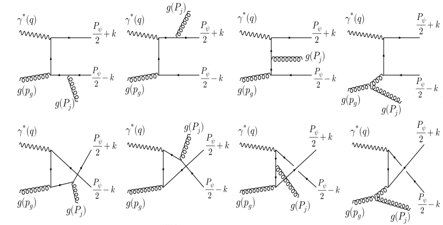
Figure 1: Feynman diagrams for the partonic process $\gamma^{*}(q)+g(p_{g})\rightarrow J/\psi(\mathrm{P}_{\psi})+g(\mathrm{P}_{j})$.

The amplitude for the production of $J/\psi$ within the NRQCD framework can be written as follows Boer and Pisano (2012a); Baier and Rückl (1983)

$$\mathcal{M}\Big{(}\gamma^{*}\leavevmode\nobreak\ g\to Q\bar{Q}[^{2S+1}L_{J}^{(1,8)}]\leavevmode\nobreak\ g\Big{)}=\sum_{L_{z}S_{z}} \int\frac{d^{3}\textbf{k}}{(2\pi)^{3}}\Psi_{LL_{z}}(\textbf{k})\langle LL_{z};SS_{z}|JJ_{z}\rangle$$ (13)

$$\times Tr[O(q,p_{g},\mathrm{P}_{\psi},k)\bm{\mathcal{P}}_{SS_{z}}(\mathrm{P}_{\psi},k)],$$

where $k$ is the relative momentum of the heavy quark or the anti-quark in the rest frame of the non-relativistic quarkonium bound state, which is assumed to be very small as compared with the rest mass of the quarkonium. Here $\Psi_{LL_{z}}(\textbf{k})$ is the nonrelativistic bound-state wave function with orbital angular momentum $L,L_{z}$. The Clebsch-Gordan coefficients $\langle LL_{z};SS_{z}|JJ_{z}\rangle$ projects out their angular momentum. The mass of the quarkonium, $M_{\psi}$, is taken to be twice the heavy quark mass. The $O(q,p_{g},\mathrm{P}_{\psi},k)$ represents the amplitude for the production of the heavy quark anti-quark pair, $Q\bar{Q}$, without the inclusion of the polarization of the quark and anti-quark. This can be calculated by considering the contributions from all the above Feynman diagrams and can be written as

$$O(q,p_{g},\mathrm{P}_{\psi},k)=\sum_{i=1}^{8}C_{i}\leavevmode\nobreak\ O_{i}(q,p_{g},\mathrm{P}_{\psi},k),$$ (14)

where, $i$ denotes the contribution from the individual Feynman diagrams given in Fig. 1 and $C_{i}$ corresponds to the color factor for each diagram. The $O_{i}(q,p_{g},\mathrm{P}_{\psi},k)$ for the above Feynman diagrams are written as

$$O_{1} = 4g_{s}^{2}(ee_{c})\varepsilon_{g}^{*\lambda}(\mathrm{P}_{j})\gamma_{\nu}\frac{\not{\mathrm{P}}_{\psi}+2\not{k}-2\not{q}+M_{\psi}}{(\mathrm{P}_{\psi}+2k-2q)^{2}-M_{\psi}^{2}}\gamma_{\mu}\frac{-\not{\mathrm{P}}_{\psi}+2\not{k}-2\not{\mathrm{P}}_{j}+M_{\psi}}{(\mathrm{P}_{\psi}-2k+2\mathrm{P}_{j})^{2}-M_{\psi}^{2}}\gamma_{\lambda},$$

$$O_{2} = 4g_{s}^{2}(ee_{c})\varepsilon_{g}^{*\lambda}(\mathrm{P}_{j})\gamma_{\lambda}\frac{\not{\mathrm{P}}_{\psi}+2\not{k}+2\not{\mathrm{P}}_{j}+M_{\psi}}{(\mathrm{P}_{\psi}+2k+2\mathrm{P}_{j})^{2}-M_{\psi}^{2}}\gamma_{\nu}\frac{-\not{\mathrm{P}}_{\psi}+2\not{k}+2\not{p}_{g}+M_{\psi}}{(\mathrm{P}_{\psi}-2k-2p_{g})^{2}-M_{\psi}^{2}}\gamma_{\mu},$$

$$O_{3} = 4g_{s}^{2}(ee_{c})\varepsilon_{g}^{*\lambda}(\mathrm{P}_{j})\gamma_{\nu}\frac{\not{\mathrm{P}}_{\psi}+2\not{k}-2\not{q}+M_{\psi}}{(\mathrm{P}_{\psi}+2k-2q)^{2}-M_{\psi}^{2}}\gamma_{\lambda}\frac{-\not{\mathrm{P}}_{\psi}+2\not{k}+2\not{p}_{g}+M_{\psi}}{(\mathrm{P}_{\psi}-2k-2p_{g})^{2}-M_{\psi}^{2}}\gamma_{\mu},$$

$$O_{4} = 4g_{s}^{2}(ee_{c})\varepsilon_{g}^{*\lambda}(\mathrm{P}_{j})\gamma_{\nu}\frac{\not{\mathrm{P}}_{\psi}+2\not{k}-2\not{q}+M_{\psi}}{(\mathrm{P}_{\psi}+2k-2q)^{2}-M_{\psi}^{2}}\gamma^{\chi}$$ (15)

$$\leavevmode\nobreak\ \leavevmode\nobreak\ \leavevmode\nobreak\ \leavevmode\nobreak\ \leavevmode\nobreak\ \leavevmode\nobreak\ \leavevmode\nobreak\ \leavevmode\nobreak\ \leavevmode\nobreak\ \leavevmode\nobreak\ \leavevmode\nobreak\ \leavevmode\nobreak\ \leavevmode\nobreak\ \leavevmode\nobreak\ \leavevmode\nobreak\ \leavevmode\nobreak\ \leavevmode\nobreak\ \leavevmode\nobreak\ \leavevmode\nobreak\ \leavevmode\nobreak\ \leavevmode\nobreak\ \leavevmode\nobreak\ \leavevmode\nobreak\ \leavevmode\nobreak\ \leavevmode\nobreak\ \leavevmode\nobreak\ \leavevmode\nobreak\ \frac{[g_{\mu\lambda}(p_{g}+\mathrm{P}_{j})_{\chi}+g_{\lambda\chi}(p_{g}-2\mathrm{P}_{j})_{\mu}+g_{\chi\mu}(\mathrm{P}_{j}-2p_{g})_{\lambda}]}{(p_{g}-\mathrm{P}_{j})^{2}}.$$

The expressions for the remaining, $O_{5},\leavevmode\nobreak\ O_{6},\leavevmode\nobreak\ O_{7}$ and $O_{8}$ can be obtained by reversing the fermionic current and replacing $k$ to $-k$.

In the NRQCD framework, the outgoing $Q\bar{Q}$ pair can be formed in the color singlet (CS) state or in the color octet (CO) states. The color factors, $C_{i}$, corresponding to the CO case are given as Rajesh et al. (2018a),

$$C_{1}=C_{6}=C_{7}=\sum_{jk}\langle 3j;\bar{3}k|8c\rangle(t_{a}t_{b})_{jk},$$

$$C_{2}=C_{3}=C_{5}=\sum_{jk}\langle 3j;\bar{3}k|8c\rangle(t_{b}t_{a})_{jk},$$

$$C_{4}=C_{8}=\sum_{jk}\langle 3j;\bar{3}k|8c\rangle if_{abd}(t_{d})_{jk}.$$ (16)

The SU(3) Clebsch-Gordon coefficients for CS and CO states are given by, respectively,

$$\langle 3j;\bar{3}k|1\rangle=\frac{\delta_{jk}}{\sqrt{N_{c}}},\leavevmode\nobreak\ \leavevmode\nobreak\ \langle 3j;\bar{3}k|8c\rangle=\sqrt{2}(t_{c})_{jk},$$ (17)

where $N_{c}$ is number of colors, $t_{c}$ is the generators of SU(3) in the fundamental representation. Their properties are given by $Tr[t_{a}t_{b}]=\delta_{ab}/2$ and $Tr[t_{a}t_{b}t_{c}]=\frac{1}{4}(d_{abc}+if_{abc})$. By using these relations along with the relation in Eq. (17), one obtains the color factors for individual Feynman diagrams for the $Q\bar{Q}$ formed in color octet states as

$$C_{1}=C_{6}=C_{7}=\frac{\sqrt{2}}{4}(d_{abc}+if_{abc}),$$

$$C_{2}=C_{3}=C_{5}=\frac{\sqrt{2}}{4}(d_{abc}-if_{abc}),$$

$$C_{4}=C_{8}=\frac{\sqrt{2}}{2}if_{abc}.$$ (18)

For the case of formation of $Q\bar{Q}$ pair in CS state, the color factors are given by

$$C_{1}=C_{2}=C_{3}=C_{5}=C_{6}=C_{7}=\frac{\delta_{ab}}{2\sqrt{N_{c}}}.$$ (19)

The spin projection operator for the bound state of the $J/\psi$ includes the spinors of the heavy quark and anti-quark, $c\bar{c}$ and is given as

$$\bm{\mathcal{P}}_{SS_{z}}(\mathrm{P}_{\psi},k) =\sum_{s_{1}s_{2}}\Big{\langle}\frac{1}{2}s_{1};\frac{1}{2}s_{2}\Big{|}SS_{z}\Big{\rangle}v\Big{(}\frac{\mathrm{P}_{\psi}}{2}-k,s_{1}\Big{)}\bar{u}\Big{(}\frac{\mathrm{P}_{\psi}}{2}+k,s_{2}\Big{)}$$ (20)

$$=\frac{1}{4M_{\psi}^{3/2}}\big{(}-\not{\mathrm{P}}_{\psi}+2\not{k}+M_{\psi}\big{)}\Pi_{SS_{z}}\big{(}\not{\mathrm{P}}_{\psi}+2\not{k}+M_{\psi}\big{)}+\mathcal{O}(k^{2}),$$

where, $\Pi_{SS_{z}}=\gamma^{5}$ for spin singlet ($S=0$) and $\Pi_{SS_{z}}=\not{\varepsilon}_{S_{z}}(\mathrm{P}_{\psi})$ for spin triplet ($S=1$). The $\varepsilon_{S_{z}}$ is the spin polarization vector of the outgoing $c\bar{c}$ pair.

Now, since, in the rest frame of the bound state, $k\ll\mathrm{P}_{\psi}$, thus one can Taylor expand the amplitude given in Eq. (13) around $k=0$ limit. In that expansion, the terms corresponding to $k^{0}$ give S-wave scattering amplitude $(L=0,\leavevmode\nobreak\ J=0,1)$ and terms linear in $k$ correspond to P-wave scattering $(L=1,\leavevmode\nobreak\ J=0,1,2)$ and the corresponding amplitudes are given as

$$\mathcal{M}[^{2S+1}S_{J}^{(1,8)}](\mathrm{P}_{\psi},k)= \frac{1}{\sqrt{4\pi}}R_{0}(0)Tr[O(q,p_{g},\mathrm{P}_{\psi},k)\bm{\mathcal{P}}_{SS_{z}}(\mathrm{P}_{\psi},k)]\Big{|}_{k=0}$$

$$= \frac{1}{\sqrt{4\pi}}R_{0}(0)Tr[O(0)\bm{\mathcal{P}}_{SS_{z}}(0)],$$ (21)

$$\mathcal{M}[^{2S+1}P_{J}^{(8)}](\mathrm{P}_{\psi},k)= -i\sqrt{\frac{3}{4\pi}}R_{1}^{\prime}(0)\sum_{L_{z}S_{z}}\varepsilon^{\alpha}_{L_{z}}(\mathrm{P}_{\psi})\langle LL_{z};SS_{z}|JJ_{z}\rangle$$

$$\times\frac{\partial}{\partial k^{\alpha}}Tr[O(q,p_{g},\mathrm{P}_{\psi},k)\bm{\mathcal{P}}_{SS_{z}}(\mathrm{P}_{\psi},k)]\Big{|}_{k=0}$$

$$= -i\sqrt{\frac{3}{4\pi}}R_{1}^{\prime}(0)\sum_{L_{z}S_{z}}\varepsilon^{\alpha}_{L_{z}}(\mathrm{P}_{\psi})\langle LL_{z};SS_{z}|JJ_{z}\rangle$$ (22)

$$\times Tr[O_{\alpha}(0)\bm{\mathcal{P}}_{SS_{z}}(0)+O(0)\bm{\mathcal{P}}_{SS_{z}\alpha}(0)].$$

Where $R_{L}$ represents the radial wave function and the shorthand notations used in the above expressions are

$$O(0)=O(q,p_{g},\mathrm{P}_{\psi},k)\Big{|}_{k=0},\leavevmode\nobreak\ \leavevmode\nobreak\ \leavevmode\nobreak\ \leavevmode\nobreak\ \leavevmode\nobreak\ \leavevmode\nobreak\ \leavevmode\nobreak\ \leavevmode\nobreak\ \leavevmode\nobreak\ \leavevmode\nobreak\ \leavevmode\nobreak\ \leavevmode\nobreak\ \leavevmode\nobreak\ \bm{\mathcal{P}}_{SS_{z}}(0)=\bm{\mathcal{P}}_{SS_{z}}(\mathrm{P}_{\psi},k)\Big{|}_{k=0},$$ (23)

$$O_{\alpha}(0)=\frac{\partial}{\partial k^{\alpha}}O(q,p_{g},\mathrm{P}_{\psi},k)\Big{|}_{k=0},\leavevmode\nobreak\ \leavevmode\nobreak\ \leavevmode\nobreak\ \leavevmode\nobreak\ \leavevmode\nobreak\ \leavevmode\nobreak\ \bm{\mathcal{P}}_{SS_{z}\alpha}(0)=\frac{\partial}{\partial k^{\alpha}}\bm{\mathcal{P}}_{SS_{z}}(\mathrm{P}_{\psi},k)\Big{|}_{k=0}.$$ (24)

Following are the relations for the Clebsch Gordon coefficient and the polarization vector of $J/\psi$ which we can use to calculate $P$ wave amplitudes Boer and Pisano (2012b)

$$\sum_{L_{z}S_{z}}\langle LL_{z};SS_{z}|JJ_{z}\rangle\varepsilon^{\alpha}_{S_{z}}(\mathrm{P}_{\psi})\varepsilon^{\beta}_{L_{z}}(\mathrm{P}_{\psi})=\sqrt{\frac{1}{3}}\Bigg{(}g^{\alpha\beta}-\frac{\mathrm{P}_{\psi}^{\alpha}\mathrm{P}_{\psi}^{\beta}}{M_{\psi}^{2}}\Bigg{)},$$ (25)

$$\sum_{L_{z}S_{z}}\langle LL_{z};SS_{z}|JJ_{z}\rangle\varepsilon^{\alpha}_{S_{z}}(\mathrm{P}_{\psi})\varepsilon^{\beta}_{L_{z}}(\mathrm{P}_{\psi})=-\frac{i}{M_{\psi}}\sqrt{\frac{1}{2}}\epsilon_{\delta\zeta\xi\varrho}g^{\xi\alpha}g^{\varrho\beta}\mathrm{P}_{\psi}^{\delta}\varepsilon^{\zeta}_{J_{z}}(\mathrm{P}_{\psi}),$$ (26)

$$\sum_{L_{z}S_{z}}\langle LL_{z};SS_{z}|JJ_{z}\rangle\varepsilon^{\alpha}_{S_{z}}(\mathrm{P}_{\psi})\varepsilon^{\beta}_{L_{z}}(\mathrm{P}_{\psi})=\varepsilon^{\alpha\beta}_{J_{z}}(\mathrm{P}_{\psi}).$$ (27)

The $\varepsilon^{\alpha}_{J_{z}}(\mathrm{P}_{\psi})$ is the polarization vector corresponding to $J=1$ angular momentum state, that follows the current conservation and obeys the following relations Boer and Pisano (2012b),

$$\varepsilon^{\alpha}_{J_{z}}(\mathrm{P}_{\psi})\mathrm{P}_{\psi\alpha} = 0,$$ (28)

$$\sum_{J_{z}}\varepsilon^{\alpha}_{J_{z}}(\mathrm{P}_{\psi})\varepsilon^{*\beta}_{J_{z}}(\mathrm{P}_{\psi}) = \Bigg{(}-g^{\alpha\beta}+\frac{\mathrm{P}_{\psi}^{\alpha}\mathrm{P}_{\psi}^{\beta}}{M_{\psi}^{2}}\Bigg{)}=\mathcal{Q}^{\alpha\beta}.$$ (29)

The $\varepsilon^{\alpha\beta}_{J_{z}}(\mathrm{P}_{\psi})$ is the polarization tensor corresponding to $J=2$ which is symmetric in the Lorentz indices and follows the relations Boer and Pisano (2012b),

$$\varepsilon^{\alpha\beta}_{J_{z}}(\mathrm{P}_{\psi})=\varepsilon^{\beta\alpha}_{J_{z}}(\mathrm{P}_{\psi})\leavevmode\nobreak\ \varepsilon^{\alpha}_{J_{z}\alpha}(\mathrm{P}_{\psi})=0\leavevmode\nobreak\ \varepsilon^{\alpha}_{J_{z}}(\mathrm{P}_{\psi})\mathrm{P}_{\psi\alpha}=0,$$

$$\varepsilon^{\alpha\beta}_{J_{z}}(\mathrm{P}_{\psi})\varepsilon^{*\mu\nu}_{J_{z}}(\mathrm{P}_{\psi})=\frac{1}{2}[\mathcal{Q}^{\alpha\mu}\mathcal{Q}^{\beta\nu}+\mathcal{Q}^{\alpha\nu}\mathcal{Q}^{\beta\mu}]-\frac{1}{3}[\mathcal{Q}^{\alpha\beta}\mathcal{Q}^{\mu\nu}].$$ (30)

The radial wave function and its derivative evaluated at origin $R_{0}(0)$, $R_{1}^{\prime}(0)$ given in Eq. (21) and Eq. (22) are related to LDMEs by the following equations D’Alesio et al. (2019),

$$\langle 0|\mathcal{O}_{1}^{J/\psi}(^{2S+1}S_{J})|0\rangle=\frac{N_{c}}{2\pi}(2J+1)|R_{0}(0)|^{2},$$ (31)

$$\langle 0|\mathcal{O}_{8}^{J/\psi}(^{2S+1}S_{J})|0\rangle=\frac{2}{\pi}(2J+1)|R_{0}(0)|^{2},$$ (32)

$$\langle 0|\mathcal{O}_{8}^{J/\psi}(^{3}P_{J})|0\rangle=\frac{2N_{c}}{\pi}(2J+1)|R^{\prime}_{1}(0)|^{2}.$$ (33)

The two different sets of LDMEs that we have used in our numerical calculation are given in Table. 1

	$\langle 0|\mathcal{O}_{8}^{J/\psi}(^{1}S_{0})|0\rangle$	$\langle 0|\mathcal{O}_{8}^{J/\psi}(^{3}S_{1})|0\rangle$	$\langle 0|\mathcal{O}_{1}^{J/\psi}(^{3}S_{1})|0\rangle$	$\langle 0|\mathcal{O}_{8}^{J/\psi}(^{3}P_{0})|0\rangle/m_{c}^{2}$
Ref. Sharma and Vitev (2013)	1.8 $\pm$ 0.87	0.13 $\pm$0.13	1.2 $\times\leavevmode\nobreak\ 10^{2}$	1.8 $\pm$ 0.87	$\times 10^{-2}$GeV3
Ref. Chao et al. (2012)	8.9 $\pm$ 0.98	0.30 $\pm$0.12	1.2 $\times\leavevmode\nobreak\ 10^{2}$	0.56 $\pm$ 0.21	$\times 10^{-2}$GeV3

Table 1: Numerical values for two different sets of LDMEs.

Now, using the aforementioned formalism, together with the symmetry relations among the amplitudes corresponding to different Feynman diagrams for each state, which have been calculated in Ref. Rajesh et al. (2018b), we could write the amplitude for the CS state $(^{3}S_{1}^{(1)})$ and CO states $(^{3}S_{1}^{(8)},\ ^{1}S_{0}^{(8)},\ ^{3}P_{J(0,1,2)}^{(8)})$ as

II.2 ${}^{3}S_{1}^{(1,8)}$ Amplitude

The final expression for ${}^{3}S_{1}^{(1)}$state and ${}^{3}S_{1}^{(8)}$ state can be written as,

$$\mathcal{M}[^{3}S_{1}^{(1)}](\mathrm{P}_{\psi},p_{g})=\frac{1}{4\sqrt{\pi M_{\psi}}}R_{0}(0)\frac{\delta_{ab}}{2\sqrt{N_{c}}}Tr\Bigg{[}\sum_{i=1}^{3}O_{i}(0)(\not{\mathrm{P}}_{\psi}+M_{\psi})\not{\varepsilon}_{S_{z}}\Bigg{]},$$ (34)

$$\mathcal{M}[^{3}S_{1}^{(8)}](\mathrm{P}_{\psi},p_{g})=\frac{1}{4\sqrt{\pi M_{\psi}}}R_{0}(0)\frac{\sqrt{2}}{2}d_{abc}Tr\Bigg{[}\sum_{i=1}^{3}O_{i}(0)(\not{\mathrm{P}}_{\psi}+M_{\psi})\not{\varepsilon}_{S_{z}}\Bigg{]}.$$ (35)

Where, $\sum_{i=1}^{3}O_{i}(0)$ is given as,

$$\sum_{i=1}^{3}O_{i}(0) =4g_{s}^{2}(ee_{c})\varepsilon_{g}^{*\lambda}\Bigg{[}\frac{\gamma_{\nu}(\not{\mathrm{P}}_{\psi}-2\not{q}+M_{\psi})\gamma_{\mu}(-\not{\mathrm{P}}_{\psi}-2\not{\mathrm{P}}_{j}+M_{\psi})\gamma_{\lambda}}{(s-M_{\psi}^{2})(u-M_{\psi}^{2}+q^{2})}$$

$$\leavevmode\nobreak\ \leavevmode\nobreak\ \leavevmode\nobreak\ \leavevmode\nobreak\ \leavevmode\nobreak\ \leavevmode\nobreak\ \leavevmode\nobreak\ \leavevmode\nobreak\ \leavevmode\nobreak\ \leavevmode\nobreak\ \leavevmode\nobreak\ \leavevmode\nobreak\ \leavevmode\nobreak\ \leavevmode\nobreak\ \leavevmode\nobreak\ \leavevmode\nobreak\ \leavevmode\nobreak\ \leavevmode\nobreak\ \leavevmode\nobreak\ \leavevmode\nobreak\ +\frac{\gamma_{\lambda}(\not{\mathrm{P}}_{\psi}+2\not{\mathrm{P}}_{j}+M_{\psi})\gamma_{\nu}(-\not{\mathrm{P}}_{\psi}+2\not{p}_{g}+M_{\psi})\gamma_{\mu}}{(s-M_{\psi}^{2})(t-M_{\psi}^{2})}$$

$$\leavevmode\nobreak\ \leavevmode\nobreak\ \leavevmode\nobreak\ \leavevmode\nobreak\ \leavevmode\nobreak\ \leavevmode\nobreak\ \leavevmode\nobreak\ \leavevmode\nobreak\ \leavevmode\nobreak\ \leavevmode\nobreak\ \leavevmode\nobreak\ \leavevmode\nobreak\ \leavevmode\nobreak\ \leavevmode\nobreak\ \leavevmode\nobreak\ \leavevmode\nobreak\ \leavevmode\nobreak\ \leavevmode\nobreak\ \leavevmode\nobreak\ \leavevmode\nobreak\ +\frac{\gamma_{\nu}(\not{\mathrm{P}}_{\psi}-2\not{q}+M_{\psi})\gamma_{\lambda}(-\not{\mathrm{P}}_{\psi}+2\not{p}_{g}+M_{\psi})\gamma_{\mu}}{(t-M_{\psi}^{2})(u-M_{\psi}^{2}+q^{2})}\Bigg{]}.$$

The symmetry relations, given in Ref. Rajesh et al. (2018b), lead to the cancellation of contributions from Feynman diagrams 4 and 8 for ${}^{3}S_{1}^{(1,8)}$ amplitude.

II.3 ${}^{1}S_{0}^{(8)}$ Amplitude

The total amplitude for ${}^{1}S_{0}^{(8)}$ state can be written as,

$$\mathcal{M}[^{1}S_{0}^{(8)}](\mathrm{P}_{\psi},p_{g})=\frac{1}{4\sqrt{\pi M_{\psi}}}R_{0}(0)i\frac{\sqrt{2}}{2}f_{abc}Tr\Big{[}(O_{1}(0)-O_{2}(0)-O_{3}(0)+2O_{4}(0))(\not{\mathrm{P}}_{\psi}+M_{\psi})\gamma_{5}\Big{]}.$$ (37)

$O_{1}(0),\leavevmode\nobreak\ O_{2}(0),\leavevmode\nobreak\ O_{3}(0)$ are given in the Eq. (LABEL:total3S1) and

$$O_{4}(0)=g_{s}^{2}(ee_{c})\varepsilon_{g}^{*\lambda}\frac{\gamma_{\nu}(\not{\mathrm{P}}_{\psi}-2\not{q}+M_{\psi})\gamma^{\chi}}{u(u-M_{\psi}^{2})}[g_{\mu\lambda}(p_{g}+\mathrm{P}_{j})_{\chi}+g_{\lambda\chi}(p_{g}-2\mathrm{P}_{j})_{\mu}+g_{\chi\mu}(\mathrm{P}_{j}-2p_{g})_{\lambda}].$$ (38)

II.4 ${}^{3}P_{J}^{(8)}$  Amplitude

The ${}^{3}P_{J}^{(8)}$ amplitude can be written as Rajesh et al. (2018b),

$$\mathcal{M}[^{3}\mathcal{P}_{J}^{(8)}](\mathrm{P}_{\psi},p_{g})= \frac{\sqrt{2}}{2}f_{abc}\sqrt{\frac{3}{4\pi}}R_{1}^{\prime}(0)\sum_{L_{z}S_{z}}\varepsilon^{\alpha}_{L_{z}}(\mathrm{P}_{\psi})\langle LL_{z};SS_{z}|JJ_{z}\rangle$$ (39)

$$Tr[(O_{1\alpha}(0)-O_{2\alpha}(0)-O_{3\alpha}(0)+2O_{4\alpha}(0))\bm{\mathcal{P}}_{SS_{z}}(0)$$

$$+(O_{1}(0)-O_{2}(0)-O_{3}(0)+2O_{4}(0))\bm{\mathcal{P}}_{SS_{z}\alpha}(0)].$$

II.5 Total differential cross-section and the asymmetry

The structure of differential cross-section as defined in Eq. (10) has a contraction of tensors which can be schematically written as

$$\mathfrak{M}_{i}\mathfrak{M}_{j}=L^{\mu\mu^{\prime}}(l,q)\Phi_{g}^{\nu\nu^{\prime}}(x,\mathbf{p}_{T})\mathcal{M}_{i\mu\nu}\mathcal{M}_{j\mu^{\prime}\nu^{\prime}},$$ (40)

where $i,j=1,2,3,4$ (corresponds to the Feynman diagrams given in Fig. 1 and we have $\mathfrak{M}_{i}\mathfrak{M}_{j}=\mathfrak{M}_{j}\mathfrak{M}_{i}$ for $i\neq j$. We have already defined all tensors in the above convolution and contributions to the amplitudes come from all the CS and CO states $(^{3}S_{1}^{(1,8)},\ ^{1}S_{0}^{(8)},\ ^{3}P_{J(0,1,2)}^{(8)})$. We have summed over all the polarization states of the outgoing gluon using the relation given as

$$\sum_{\lambda_{a}=1}^{2}\varepsilon^{\lambda_{a}}_{\mu}\varepsilon^{\lambda_{a}}_{\mu^{\prime}}=-g_{\mu\mu^{\prime}}+\frac{\mathrm{P}_{j\mu}n_{\psi\mu^{\prime}}+\mathrm{P}_{j\mu^{\prime}}n_{\psi\mu}}{\mathrm{P}_{j}\cdot n_{\psi}}-\frac{\mathrm{P}_{j\mu}\mathrm{P}_{j\mu^{\prime}}}{(\mathrm{P}_{j}\cdot n_{\psi})^{2}},$$ (41)

where, $n_{\psi\mu}=\mathrm{P}_{\psi\mu}/M_{\psi}$. We use the frame where the incoming virtual photon and proton moves along $z$-axis. The azimuthal angles of the lepton scattering plane is defined as $\phi_{l}=\phi_{l^{\prime}}=0$. We integrate out the azimuthal angle of the final lepton $\ell^{\prime}$  Graudenz (1994), we can write

$$\frac{\mathrm{d}^{3}\ell^{\prime}}{(2\pi)^{3}2E_{\ell^{\prime}}}=\frac{\mathrm{d}Q^{2}\mathrm{d}y}{16\pi^{2}}.$$ (42)

Moreover, for the other phase factors, one can write

$$\frac{\mathrm{d}^{3}\mathrm{P}_{\psi}}{(2\pi)^{3}2E_{\psi}}=\frac{\mathrm{d}z\mathrm{d}^{2}\bm{\mathrm{P}}_{\psi\perp}}{(2\pi)^{3}2z}\;,\quad\frac{\mathrm{d}^{3}\mathrm{P}_{j}}{(2\pi)^{3}2E_{j}}=\frac{\mathrm{d}\bar{z}\mathrm{d}^{2}\bm{\mathrm{P}}_{j\perp}}{(2\pi)^{3}2\bar{z}}\;,$$ (43)

and conservation of the four-momenta can be written as

$$\delta^{4}\big{(}q+p_{g}-\mathrm{P}_{\psi}-\mathrm{P}_{j}\big{)}$$ (44)

$$=\frac{2}{ys}\delta\bigl{(}1-z-\bar{z}\bigr{)}\delta\left(x-\frac{\bar{z}(M^{2}+\bm{\mathrm{P}}_{\psi\perp}^{2})+z\bm{\mathrm{P}}_{j\perp}^{2}+z\bar{z}Q^{2}}{z(1-z)ys}\right)\delta^{2}\bigl{(}\bm{\mathrm{p}}_{{\scriptscriptstyle T}}-\bm{\mathrm{P}}_{j\perp}-\bm{\mathrm{P}}_{\psi\perp}\bigr{)}\;,$$

where we have used the relation $Q^{2}=x_{B}ys$. Now, we define the sum and difference of the transverse momentum of $J/\psi$ and jet as

$$\bm{\mathrm{q}}_{t} \equiv\bm{\mathrm{P}}_{\psi\perp}+\bm{\mathrm{P}}_{j\perp}\,,\quad\bm{\mathrm{K}}_{t}\equiv\frac{\bm{\mathrm{P}}_{\psi\perp}-\bm{\mathrm{P}}_{j\perp}}{2}\,.$$ (45)

From Eq. (44), we have $\bar{z}=(1-z)$ and $\textbf{q}_{t}=\textbf{p}_{T}$. We use TMD factorization in the kinematic region $|\textbf{q}_{t}|\ll|\textbf{K}_{t}|$. This leads to the situation where the outgoing $J/\psi$ and jet are almost back to back in the transverse plane, $i.e.$ the $xy$ plane, w.r.t the virtual photon-proton colliding axis, $i.e.$ the $z$-axis, thus allowing us to set $\textbf{K}_{t}\simeq\textbf{P}_{\psi\perp}\simeq-\textbf{P}_{j\perp}$. $\phi_{t}$ and $\phi_{\perp}$ are the azimuthal angles, respectively, for $\textbf{q}_{t}$ and $\textbf{K}_{t}$ and are defined with respect to the leptonic plane as illustrated in Fig. 2.

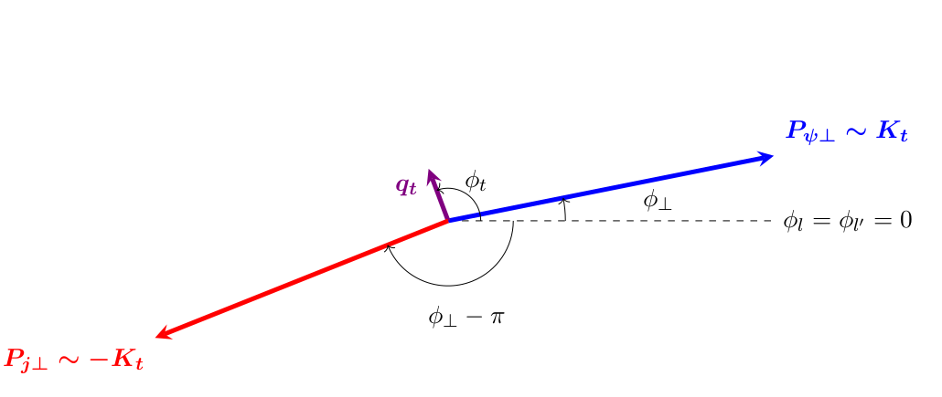
Figure 2: The schematic representation of back to back $J/\psi$ and jet production in transverse plane.

Finally, integrating over $\bar{z}$, $\bm{\mathrm{p}}_{{}_{T}}$ and $x$, the differential cross-section, in Eq. (10), as a function of $z,\ y,\ x_{B},\ \bm{\mathrm{q}}_{t},\ \bm{\mathrm{K}}_{t}$ can be rewritten as

$$\frac{\mathrm{d}\sigma}{\mathrm{d}z\,\mathrm{d}y\,\mathrm{d}x_{\scriptscriptstyle B}\,\mathrm{d}^{2}\bm{\mathrm{q}}_{t}\mathrm{d}^{2}\bm{\mathrm{K}}_{t}} =\frac{1}{(2\pi)^{4}}\frac{1}{16sz(1-z)Q^{4}}\sum_{i,j}\mathfrak{M}_{i}\mathfrak{M}_{j}.$$ (46)

In the following calculation, we have only kept the zeroth and first order terms in $\Big{(}\frac{\bm{\mathrm{q}}_{t}^{2}}{M_{P}^{2}}\Big{)}$. Thus, we obtain the total differential cross-section D’Alesio et al. (2019),

$$\frac{\mathrm{d}\sigma}{\mathrm{d}z\,\mathrm{d}y\,\mathrm{d}x_{\scriptscriptstyle B}\,\mathrm{d}^{2}\bm{\mathrm{q}}_{t}\,\mathrm{d}^{2}\bm{\mathrm{K}}_{t}} =\frac{1}{(2\pi)^{4}}\frac{1}{16sz(1-z)Q^{4}}\Big{\{}\big{(}\mathbb{A}_{0}+\mathbb{A}_{1}\cos\phi_{\perp}+\mathbb{A}_{2}\cos 2\phi_{\perp}\big{)}f_{1}^{g}(x,\bm{\mathrm{q}}_{t}^{2})+$$ (47)

$$\frac{\bm{\mathrm{q}}_{t}^{2}}{M_{P}^{2}}h_{1}^{\perp g}(x,\bm{\mathrm{q}}_{t}^{2})\big{(}\mathbb{B}_{0}\cos 2\phi_{t}+\mathbb{B}_{1}\cos(2\phi_{t}-\phi_{\perp})+\mathbb{B}_{2}\cos 2(\phi_{t}-\phi_{\perp})+$$

$$\mathbb{B}_{3}\cos(2\phi_{t}-3\phi_{\perp})+\mathbb{B}_{4}\cos(2\phi_{t}-4\phi_{\perp})\big{)}\Big{\}}.$$

The analytic expressions of the coefficients $\mathbb{A}_{i}$’s and $\mathbb{B}_{i}$’s are very lengthy, which we have not included in this article. They are available upon request.

The TMDs come with various azimuthal modulations. These modulations can be used to extract information about the ratio of TMDs. This can be done by defining the asymmetries as D’Alesio et al. (2019)

$$A^{\mathcal{W}(\phi_{S},\phi_{t})}\equiv 2\frac{\int\mathrm{d}\phi_{S}\leavevmode\nobreak\ \mathrm{d}\phi_{t}\mathrm{d}\phi_{\perp}\mathcal{W}(\phi_{S},\phi_{t})\leavevmode\nobreak\ \mathrm{d}\sigma(\phi_{S},\phi_{t},\phi_{\perp})}{\int\mathrm{d}\phi_{S}\leavevmode\nobreak\ \mathrm{d}\phi_{t}\leavevmode\nobreak\ \mathrm{d}\phi_{\perp}\leavevmode\nobreak\ \mathrm{d}\sigma(\phi_{S},\phi_{t},\phi_{\perp})}.$$ (48)

Here, we are interested in one particular asymmetry, i.e., $\cos 2\phi_{t}$ asymmetry to extract the linearly polarized gluon TMD. This can be written as,

$$\langle\cos 2\phi_{t}\rangle\equiv A^{\cos 2\phi_{t}}=2\frac{\int\mathrm{d}\phi_{t}\mathrm{d}\phi_{\perp}\cos 2\phi_{t}\mathrm{d}\sigma(\phi_{t},\phi_{\perp})}{\int\mathrm{d}\phi_{t}\mathrm{d}\phi_{\perp}\mathrm{d}\sigma(\phi_{t},\phi_{\perp})}.$$ (49)

Now, by plugging the differential scattering cross-section from Eq. (47) in the above equation, we get the $\cos 2\phi_{t}$ asymmetry as function of $z,\ y,\ x_{B},\mathrm{K}_{t}$

$$\langle\cos 2\phi_{t}\rangle\equiv A^{\cos 2\phi_{t}}=\frac{\int\mathrm{q}_{t}\leavevmode\nobreak\ \mathrm{d}\mathrm{q}_{t}\leavevmode\nobreak\ \frac{\textbf{q}_{t}^{2}}{M_{p}^{2}}\leavevmode\nobreak\ \mathbb{B}_{0}\leavevmode\nobreak\ h_{1}^{\perp g}(x,\textbf{q}_{t}^{2})}{\int\mathrm{q}_{t}\leavevmode\nobreak\ \mathrm{d}\mathrm{q}_{t}\leavevmode\nobreak\ \mathbb{A}_{0}\leavevmode\nobreak\ f_{1}^{g}(x,\textbf{q}_{t}^{2})}.$$ (50)

For estimating the $\cos 2\phi_{t}$ asymmetry numerically, we have used two recent parameterizations of the gluon TMDs, and also estimated the effect of TMD evolution. The following section gives the details of the TMD evolution formalism used.

III TMD evolution

The evolution of the TMDs Aybat and Rogers (2011a); Aybat et al. (2012a) with the scale affects the asymmetries measured in the energies of different experiments, and it is important to estimate the effect of this evolution to obtain the angular asymmetries of produced hadrons measured by the HERMES, COMPASS, JLab as well as the future EIC experiments at different energies. The TMD evolution is usually studied in the impact parameter space Aybat and Rogers (2011a). The impact parameter dependent TMDs can be written as Fourier transforms of the TMDs,

$$\hat{f}(x,\bm{\mathrm{b}}_{t}^{2};Q_{f}^{2}) = \frac{1}{2\pi}\int d^{2}\bm{\mathrm{q}}_{t}\leavevmode\nobreak\ e^{i\bm{\mathrm{q}}_{t}\cdot\bm{\mathrm{b}}_{t}}\leavevmode\nobreak\ f(x,\bm{\mathrm{q}}_{t}^{2},Q_{f}^{2}).$$ (51)

In the TMD evolution approach, TMDs not only evolve with the intrinsic transverse momentum of the parton but also evolve with the probing scale. The expression for TMD evolution at a given final scale $Q_{f}$ can be obtained by solving Collins-Soper evolution equation and renormalization group equation. Using this approach, the expression for the gluon TMD in the impact parameter space can be written as Echevarria et al. (2014a); Aybat et al. (2012b); Collins (2011)

$$\hat{f}(x,\bm{\mathrm{b}}_{t}^{2},Q_{f}^{2})=\frac{1}{2\pi}\sum_{p=q,\bar{q},g}(C_{g/p}\otimes f^{p}_{1})(x,Q_{i}^{2})e^{-\frac{1}{2}S_{A}(\bm{\mathrm{b}}_{t}^{2},Q_{f}^{2},Q_{i}^{2})}e^{-S_{np}(\bm{\mathrm{b}}_{t}^{2},Q_{f}^{2})},$$ (52)

where $Q_{i}$ is the initial scale of TMD, defined in terms of $\mathrm{b}_{t}$ as, $Q_{i}=2e^{-\gamma_{E}}/\mathrm{b}_{t}$ and $\gamma_{E}\approx 0.577$. $C_{g/p}$ are coefficient functions and $f^{p}_{1}(x,Q^{2})$ are collinear parton distributions for a species of partons like quark/anti-quark or gluon. The exponents $S_{A}$ and $S_{np}$ are the perturbative and non-perturbative Sudakov factors, respectively. We note that the Sudakov factor $S_{A}$ is spin independent, and thus the same for all (un)polarized TMDs Echevarria et al. (2015); Echevarria et al. (2014b). As stated before, a formal proof of TMD factorization for this process remains to be done, and here we study the effect of TMD evolution on the asymmetry assuming such factorization. The subsections below contain a description of the TMD evolution formalism used and the relevant formulas.

III.1 Coefficient functions and perturbative Sudakov factor

The coefficient function can be written as a series of strong coupling constant $\alpha_{s}$Boer et al. (2020),

$$C_{g/p}(x,Q_{i})=\delta_{gp}\delta(1-x)+\sum_{k=1}^{\infty}\sum_{p=g,q,\bar{q}}C^{k}_{g/p}(x)\Bigg{(}\frac{\alpha_{s}(Q_{i})}{\pi}\Bigg{)}^{k}.$$ (53)

The Sudakov factor as the leading order of $\alpha_{s}$ can be written asBoer et al. (2020),

$$S_{A}(\bm{\mathrm{b}}_{t}^{2},Q_{f}^{2},Q_{i}^{2}) = \frac{C_{A}}{\pi}\int^{Q_{f}^{2}}_{Q_{i}^{2}}\frac{d\eta^{2}}{\eta^{2}}\alpha_{s}(\eta)\Bigg{(}\log\frac{Q_{f}^{2}}{\eta^{2}}-\frac{11-2n_{f}/C_{A}}{6}\Bigg{)}$$ (54)

$$= \frac{C_{A}}{\pi}\alpha_{s}\Bigg{(}\frac{1}{2}\leavevmode\nobreak\ \log^{2}\frac{Q_{f}^{2}}{Q_{i}^{2}}-\frac{11-2n_{f}/C_{A}}{6}\leavevmode\nobreak\ \log\frac{Q_{f}^{2}}{Q_{i}^{2}}\Bigg{)}.$$

The running of the coupling $\alpha_{s}$ is ignored in Eq. (54) because it starts at $\alpha_{s}^{2}$. The $C_{A}=N_{c}$, $n_{f}$ denotes the number of active flavours. In $\mathrm{b}_{t}\ll 1/\Lambda_{QCD}$ the Sudakov factor can be Taylor expanded. Further, by substituting the expressions from Eq. (53) and Eq. (54) the unpolarized gluon TMD at LO without non-perturbative Sudakov factor is given as Boer et al. (2020),

$$\hat{f}_{1}^{g}(x,\bm{\mathrm{b}}_{t}^{2};Q_{f}^{2})= \frac{1}{2\pi}\Bigg{\{}f_{1}^{g}(x,Q_{i}^{2})-\frac{\alpha_{s}}{2\pi}\Bigg{(}\Bigg{[}\frac{C_{A}}{2}\leavevmode\nobreak\ \log^{2}\frac{Q_{f}^{2}}{Q_{i}^{2}}-\frac{11-2n_{f}/C_{A}}{6}\leavevmode\nobreak\ \log\frac{Q_{f}^{2}}{Q_{i}^{2}}\Bigg{]}f^{g}_{1}(x,Q_{i}^{2})$$ (55)

$$\leavevmode\nobreak\ \leavevmode\nobreak\ \leavevmode\nobreak\ \leavevmode\nobreak\ \leavevmode\nobreak\ \leavevmode\nobreak\ \leavevmode\nobreak\ \leavevmode\nobreak\ \leavevmode\nobreak\ \leavevmode\nobreak\ \leavevmode\nobreak\ \leavevmode\nobreak\ \leavevmode\nobreak\ \leavevmode\nobreak\ \leavevmode\nobreak\ \leavevmode\nobreak\ \leavevmode\nobreak\ \leavevmode\nobreak\ \leavevmode\nobreak\ \leavevmode\nobreak\ \leavevmode\nobreak\ \leavevmode\nobreak\ \leavevmode\nobreak\ \leavevmode\nobreak\ \leavevmode\nobreak\ \leavevmode\nobreak\ \leavevmode\nobreak\ \leavevmode\nobreak\ \leavevmode\nobreak\ \leavevmode\nobreak\ \leavevmode\nobreak\ \leavevmode\nobreak\ \leavevmode\nobreak\ \leavevmode\nobreak\ \leavevmode\nobreak\ \leavevmode\nobreak\ \leavevmode\nobreak\ -2\sum_{p}(C^{1}_{g/p}\otimes f_{1}^{p})(x,Q_{i}^{2})\Bigg{)}\Bigg{\}}.$$

Scale evolution of the collinear PDFs are given by the Dokshitzer-Gribov-Lipatov-Altarelli-Parisi (DGLAP) equation. Using this evolution equation, one can evolve $f_{1}^{g}(x,Q_{i}^{2})$ from the initial scale $Q_{i}$ to the final scale $Q_{f}$ where, $Q_{i}<Q_{f}$

$$f_{1}^{g}(x,Q_{i}^{2})=f_{1}^{g}(x,Q_{f}^{2})-\frac{\alpha_{s}}{2\pi}(P_{gg}\otimes f_{1}^{g}+P_{gi}\otimes f_{1}^{i})(x,Q_{f}^{2})\leavevmode\nobreak\ \log\frac{Q_{f}^{2}}{Q_{i}^{2}}+\mathcal{O}(\alpha_{s}^{2}).$$ (56)

Here, $P_{gg}$ and $P_{gi}$ are leading order splitting functions which are given as,

$$P_{gg}(\hat{x})=2C_{A}\Big{[}\frac{\hat{x}}{(1-\hat{x})_{+}}+\frac{1-\hat{x}}{\hat{x}}+\hat{x}(1-\hat{x})\Big{]}+\delta(1-\hat{x})\frac{11C_{A}-4n_{f}T_{R}}{6},$$ (57)

$$P_{gq}(\hat{x})=P_{g\bar{q}}(\hat{x})=C_{F}\frac{1+(1-\hat{x})^{2}}{\hat{x}}\ .$$ (58)

Where, $C_{F}=(N_{c}^{2}-1)/2N_{c}$ and $T_{R}=1/2$. In Eq. (57), the first term involves the plus prescription and thus avoids an infrared divergence because of $(1-\hat{x})$ in denominator. The plus prescription is given as Boer et al. (2020),

$$\int_{y}^{1}dz\frac{G(z)}{(1-z)_{+}}=\int_{y}^{1}dz\frac{G(z)-G(1)}{1-z}-G(1)\log{\Bigg{(}\frac{1}{1-z}\Bigg{)}}.$$ (59)

The $\otimes$ symbol denotes convolution of the two quantities;

$$(P_{gg}\otimes f_{1}^{g})(x,Q^{2})=\int_{x}^{1}\frac{d\hat{x}}{\hat{x}}\leavevmode\nobreak\ P(\hat{x},Q^{2})\leavevmode\nobreak\ f\Big{(}\frac{x}{\hat{x}},Q^{2}\Big{)}.$$ (60)

After convolution and substitution of the Eq. (56) in the Eq. (55), we have the final equation for the unpolarized gluon TMD as,

$$\hat{f}_{1}^{g}(x,\bm{\mathrm{b}}_{t}^{2};Q_{f}^{2})= \frac{1}{2\pi}\Bigg{\{}f_{1}^{g}(x,Q_{f}^{2})-\frac{\alpha_{s}}{2\pi}\Bigg{[}\Bigg{(}\frac{C_{A}}{2}\leavevmode\nobreak\ \log^{2}\frac{Q_{f}^{2}}{Q_{i}^{2}}-\frac{11C_{A}-2n_{f}}{6}\leavevmode\nobreak\ \log\frac{Q_{f}^{2}}{Q_{i}^{2}}\Bigg{)}f^{g}_{1}(x,Q_{f}^{2})$$ (61)

$$\leavevmode\nobreak\ \leavevmode\nobreak\ \leavevmode\nobreak\ \leavevmode\nobreak\ \leavevmode\nobreak\ \leavevmode\nobreak\ \leavevmode\nobreak\ \leavevmode\nobreak\ \leavevmode\nobreak\ \leavevmode\nobreak\ \leavevmode\nobreak\ \leavevmode\nobreak\ \leavevmode\nobreak\ \leavevmode\nobreak\ \leavevmode\nobreak\ \leavevmode\nobreak\ \leavevmode\nobreak\ +(P_{gg}\otimes f_{1}^{g}+P_{gi}\otimes f_{1}^{i})(x,Q_{f}^{2})\leavevmode\nobreak\ \log\frac{Q_{f}^{2}}{Q_{i}^{2}}-2f_{1}^{g}(x,Q_{f}^{2})\Bigg{]}\Bigg{\}}.$$

Now, we can write the above equation in the $\bm{\mathrm{q}}_{t}$-space by making one-to-one correspondence between the functions in impact parameter and momentum space using a general formula Tangerman and Mulders (1995); van Daal (2016); Echevarria et al. (2015)

$$\hat{f}^{(n)}(x,\bm{\mathrm{b}}_{t}^{2})\equiv\frac{2\pi n!}{M^{2n}}\int_{0}^{\infty}d\mathrm{q_{t}}\mathrm{q_{t}}\left(\frac{\mathrm{q_{t}}}{\mathrm{\mathrm{b}_{t}}}\right)^{n}J_{n}(\mathrm{q_{t}}\mathrm{\mathrm{b}_{t}})f(x,\bm{\mathrm{q}}_{t}^{2}),$$ (62)

here, $n$ is the rank of function in $\bm{\mathrm{q_{t}}}$-space. Since the unpolarized vector-meson production generally has a rank-zero structure, we can write the unpolarized gluon TMD together with the non-perturbative Sudakov factor in terms of $\bm{\mathrm{q_{t}}}$-space as

$$f_{1}^{g}(x,\bm{\mathrm{q}}_{t}^{2})=\frac{1}{2\pi} \int^{\infty}_{0}\mathrm{b}_{t}d\mathrm{b}_{t}J_{0}(\mathrm{b}_{t}\mathrm{q}_{t})\Bigg{\{}f_{1}^{g}(x,Q_{f}^{2})$$ (63)

$$\leavevmode\nobreak\ \leavevmode\nobreak\ \leavevmode\nobreak\ -\frac{\alpha_{s}}{2\pi}\Bigg{[}\Bigg{(}\frac{C_{A}}{2}\leavevmode\nobreak\ \log^{2}\frac{Q_{f}^{2}}{Q_{i}^{2}}-\frac{11C_{A}-2n_{f}}{6}\leavevmode\nobreak\ \log\frac{Q_{f}^{2}}{Q_{i}^{2}}\Bigg{)}f^{g}_{1}(x,Q_{f}^{2})$$

$$\leavevmode\nobreak\ \leavevmode\nobreak\ \leavevmode\nobreak\ \leavevmode\nobreak\ +(P_{gg}\otimes f_{1}^{g}+P_{gi}\otimes f_{1}^{i})(x,Q_{f}^{2})\leavevmode\nobreak\ \log\frac{Q_{f}^{2}}{Q_{i}^{2}}-2f_{1}^{g}(x,Q_{f}^{2})\Bigg{]}\Bigg{\}}\times e^{-S_{np}(\bm{\mathrm{b}}_{t}^{2})}.$$

Now let us write the expression for the linearly polarized gluon distribution function $h_{1}^{\perp g}(x,\bm{\mathrm{b}}_{t}^{2})$. The perturbative tail of $h_{1}^{\perp g}$ can be computed in the same way as the perturbative tail of $f_{1}^{g}$, with the key difference that its expansion in powers of the QCD coupling constant begins at $\mathrm{O}(\alpha_{s})$. Using Eq. (3.13) of Ref. Boer et al. (2020) and then performing the Fourier transformation using Eq. (62), we write the linearly polarized gluon distribution at LO in terms of the unpolarized collinear PDFs $f_{1}^{a}(\hat{x},Q_{f}^{2})$ in the $\bm{\mathrm{b}}_{t}$-space as,

$$h_{1}^{\perp g(2)}(x,\bm{\mathrm{b}}_{t}^{2};Q_{f}^{2})= \frac{2\alpha_{S}}{\pi^{2}M_{p}^{2}}\frac{1}{\bm{\mathrm{b}}_{t}^{2}}\Bigg{[}C_{A}\int_{x}^{1}\frac{d\hat{x}}{\hat{x}}\Bigg{(}\frac{\hat{x}}{x}-1\Bigg{)}f_{1}^{g}(\hat{x},Q_{f}^{2})$$ (64)

$$\leavevmode\nobreak\ \leavevmode\nobreak\ \leavevmode\nobreak\ \leavevmode\nobreak\ \leavevmode\nobreak\ \leavevmode\nobreak\ \leavevmode\nobreak\ \leavevmode\nobreak\ \leavevmode\nobreak\ \leavevmode\nobreak\ \leavevmode\nobreak\ \leavevmode\nobreak\ \leavevmode\nobreak\ \leavevmode\nobreak\ \leavevmode\nobreak\ \leavevmode\nobreak\ \leavevmode\nobreak\ \leavevmode\nobreak\ \leavevmode\nobreak\ \leavevmode\nobreak\ +C_{F}\sum_{p=q,\bar{q}}\int_{x}^{1}\frac{d\hat{x}}{\hat{x}}\Bigg{(}\frac{\hat{x}}{x}-1\Bigg{)}f_{1}^{p}(\hat{x},Q_{f}^{2})\Bigg{]}.$$

Here we have used the general formula for Bessel integral Kovchegov and Levin (2012)

$$\int_{0}^{\infty}dk\leavevmode\nobreak\ k^{\lambda-1}\leavevmode\nobreak\ J_{\nu}(kx)=2^{\lambda-1}x^{-\lambda}\frac{\Gamma(1/2(\nu+\lambda))}{\Gamma(1/2(2+\nu+\lambda))},$$ (65)

where $J_{\nu}(z)$ is the Bessel function of the first kind of order $\nu$. The $\mathrm{q}_{t}$ dependence for $h_{1}^{\perp g}$ in the gluon correlator has a rank-two tensor structure in the non-contracted transverse momentum, thus we could write the linearly polarized gluon TMD $h_{1}^{\perp g}$ in the $\bm{\mathrm{q}}_{t}$-space is given as,

$$\frac{\bm{\mathrm{q}}_{t}^{2}}{M_{p}^{2}}h_{1}^{\perp g(2)}(x,\bm{\mathrm{q}}_{t}^{2})= \frac{\alpha_{s}}{\pi^{2}}\int_{0}^{\infty}d{\mathrm{b_{t}}}{\mathrm{b_{t}}}\leavevmode\nobreak\ J_{2}(\mathrm{q_{t}}\mathrm{b_{t}})\leavevmode\nobreak\ \Bigg{[}C_{A}\int_{x}^{1}\frac{d\hat{x}}{\hat{x}}\Bigg{(}\frac{\hat{x}}{x}-1\Bigg{)}f_{1}^{g}(\hat{x},Q_{f}^{2})$$ (66)

$$\leavevmode\nobreak\ \leavevmode\nobreak\ \leavevmode\nobreak\ \leavevmode\nobreak\ \leavevmode\nobreak\ \leavevmode\nobreak\ \leavevmode\nobreak\ \leavevmode\nobreak\ \leavevmode\nobreak\ \leavevmode\nobreak\ \leavevmode\nobreak\ \leavevmode\nobreak\ \leavevmode\nobreak\ \leavevmode\nobreak\ \leavevmode\nobreak\ \leavevmode\nobreak\ \leavevmode\nobreak\ \leavevmode\nobreak\ \leavevmode\nobreak\ \leavevmode\nobreak\ +C_{F}\sum_{p=q,\bar{q}}\int_{x}^{1}\frac{d\hat{x}}{\hat{x}}\Bigg{(}\frac{\hat{x}}{x}-1\Bigg{)}f_{1}^{p}(\hat{x},Q_{f}^{2})\Bigg{]}\times e^{-S_{np}(\bm{\mathrm{b_{t}}}^{2})}.$$

III.2 Non-perturbative Sudakov factor

In the above Eqs. 63 and 66, the perturbative part is strictly valid in the perturbative domain, which means low $\mathrm{b}_{t}$ (or $\mathrm{b}_{t}<<1/\Lambda_{QCD}$). However, in order to perform the corresponding Fourier transform, we need to integrate the expression from small to large $\mathrm{b}_{t}$. As a result, the perturbative expression for the Sudakov factor given above should not be used alone rather one needs to introduce a non-perturbative Sudakov factor, this should suppress the large $\mathrm{b}_{t}$ domain. The functional form of the non-perturbative Sudakov factor is constrained by two conditions, one of which is it has to be equal to $1$ for $\mathrm{b}_{t}=0$ and for large $\mathrm{b}_{t}$ it is supposed to decrease monotonically and ultimately should vanish. The functional form attributed to $S_{np}$ is quadratic in $\mathrm{b}_{t}$ with $e^{-S_{np}}$ reaching 0 within a certain value of $\mathrm{b}_{t}$ called $\mathrm{b}_{t\text{lim}}$. However, when $\mathrm{b}_{t}$ gets too small, the lower scale $Q_{i}=2e^{-\gamma_{E}}/\mathrm{b}_{t}$ will be larger than final scale $Q_{f}$ and hence, we expect the evolution should stop. This could be resolved by taking a $\mathrm{b}_{t}$ prescription as given below Scarpa et al. (2020),

$$b_{t\star}(\mathrm{b}_{c}(\mathrm{b}_{t}))=\frac{\mathrm{b}_{c}(\mathrm{b}_{t})}{\sqrt{1+\frac{b_{c}(\mathrm{b}_{t})}{b_{t\text{max}}}}}$$ (67)

where,

$$\mathrm{b}_{c}=\sqrt{\mathrm{b}_{t}^{2}+\Big{(}\frac{2e^{-\gamma_{E}}}{Q_{f}}\Big{)}^{2}}.$$

This prescription constrains the $Q_{i}(\mathrm{b}_{t})=2\gamma_{E}/b_{t\star}(\mathrm{b}_{t})$ range in between $2\gamma_{E}/\mathrm{b}_{t\text{max}}$ (for $\mathrm{b}_{t}\to\infty$) and $Q_{f}$ (for $\mathrm{b}_{t}\to 0$). Motivated by Scarpa et al. (2020) we choose the Gaussian behavior of $e^{-S_{np}}$ as ,

$$S_{np}=\frac{A}{2}\log{\Big{(}\frac{Q_{f}}{Q_{np}}\Big{)}}\mathrm{b}_{c}^{2},\leavevmode\nobreak\ \leavevmode\nobreak\ \leavevmode\nobreak\ \leavevmode\nobreak\ \leavevmode\nobreak\ \leavevmode\nobreak\ \leavevmode\nobreak\ \leavevmode\nobreak\ \leavevmode\nobreak\ \quad Q_{np}=1\leavevmode\nobreak\ \mathrm{GeV}.$$ (68)

The parameter $A$ controls the width of the non-perturbative Sudakov factor for a particular $Q_{f}$. In this calculation, we have taken the final scale as $Q_{f}=\sqrt{M_{\psi}^{2}+\mathrm{K}_{t}^{2}}$. We have taken $A=2.3$ GeV², which is calculated for $\mathrm{K}_{t}=1\leavevmode\nobreak\ \mathrm{GeV}$. The $\mathrm{K}_{t}$ dependence present in $Q_{f}$ does not affect the value of $A$, as $\mathrm{K}_{t}$ increases the $e^{-S_{np}}$ remains below the convergence criteria at the given $\mathrm{b}_{t\text{lim}}$. The value of $\mathrm{b}_{t\text{max}}$ for the following numerical study is $1.5\leavevmode\nobreak\ \mathrm{GeV}^{-1}$ which is in consistent with Scarpa et al. (2020), Collins-Soper-Sterman formalism given for Z Boson production Landry et al. (2003) and Collins-Soper-Sterman formalism implemented by Aybat and Rogers (2011b). Below we present two recent parameterizations of the gluon TMDs that we have used.

IV Spectator model

In this section, we discuss a recent parameterization of the gluon TMDs based on a spectator model Bacchetta et al. (2020). According to this model, the remnant after the gluon emission from the nucleon is treated as a single spectator particle, which is on-shell, with mass $M_{X}$. The mass can take a range of values given by a spectral function. The nucleon-gluon-spectator coupling is encoded in an effective vertex that contains two form factors. The expression for a given TMD reads as

$$F^{g}(x,\bm{\mathrm{q}}_{t}^{2})=\int_{M}^{\infty}dM_{X}\,\rho_{X}(M_{X})\,\hat{F}^{g}(x,\bm{\mathrm{q}}_{t}^{2};M_{X})\;.$$ (69)

Here $\rho_{X}(M_{X})$ is the spectral function and can be written as

$$\rho_{X}(M_{X})=\mu^{2a}\left[\frac{A}{B+\mu^{2b}}+\frac{C}{\pi\sigma}e^{-\frac{(M_{X}-D)^{2}}{\sigma^{2}}}\right]\;.$$ (70)

Where $\mu=M_{X}^{2}-M^{2}$ and $\{X\}\equiv\{A,B,a,b,C,D,\sigma\}$ are free parameters. The parameter B in the above equation is set at $B=2.1$ and $M_{X}$ can take real values in the continuous range according to the above spectral function. The nucleon mass M is taken to be 1. The parameters a, b have a strong influence on the spectral function, at larger $M_{X}$, its asymptotic trend depends on the sign of the difference $a-b$ Bacchetta et al. (2020). For $a-b<0$, the value of $\rho_{X}$ approaches zero for large $M_{X}$. We consider integration in Eq.(69) over the range $1<M_{X}<10$ GeV. The value of different parameters that we used for our numerical results are given in the Table 2 below. These model parameters have been fixed by fitting the NNPDF data at scale $Q=1.64$ GeV Bacchetta et al. (2020). We assumed the same set of parameters to probe the TMDs at $Q=\sqrt{M_{\psi}^{2}+\mathrm{K}_{t}^{2}}$. In this model, we don’t have direct inference of scale dependency on the TMDs unlike the case of Gaussian parameterization. However, the longitudinal momentum fraction $x$ depends on $Q$ but going from some low $Q=1.64$ GeV to some relatively large $Q=\sqrt{M_{\psi}+\mathrm{K}_{t}^{2}}$ ($\approx 6.75$ GeV for $M_{\psi}=3.1$ GeV and $\mathrm{K}_{t}=6$ GeV) hardly changes the $x$ range.

Parameter	Replica 11	Parameter	Replica 11
$A$	6.0	$\kappa_{2}$ (GeV2)	0.414
$a$	0.78	$\sigma$ (GeV)	0.50
$b$	1.38	$\Lambda_{X}$ (GeV)	0.448
$C$	346	$\kappa_{1}$ (GeV2)	1.46
$D$ (GeV)	0.548

Table 2: Corresponding values for replica 11.

The leading-twist T -even unpolarized and linearly polarized gluon TMDs can be written asMulders and Rodrigues (2001); Meissner et al. (2007)

$$\hat{f}_{1}^{g}(x,\bm{\mathrm{q}}_{t}^{2};M_{X}) = -\frac{1}{2}\,g^{ij}\,\left[\Phi^{ij}(x,\bm{\mathrm{q}}_{t},S)+\Phi^{ij}(x,\bm{\mathrm{q}}_{t},-S)\right]$$ (71)

$$= \Big{[}\big{(}2Mxg_{1}-x(M+M_{X})g_{2}\big{)}^{2}\,\big{[}(M_{X}-M(1-x))^{2}+\bm{\mathrm{q}}_{t}^{2}\big{]}$$

$$\leavevmode\nobreak\ \leavevmode\nobreak\ \leavevmode\nobreak\ \leavevmode\nobreak\ \leavevmode\nobreak\ \leavevmode\nobreak\ \leavevmode\nobreak\ \leavevmode\nobreak\ \leavevmode\nobreak\ \leavevmode\nobreak\ \leavevmode\nobreak\ +2\bm{\mathrm{q}}_{t}^{2}\,(\bm{\mathrm{q}}_{t}^{2}+xM_{X}^{2})\,g_{2}^{2}+2\bm{\mathrm{q}}_{t}^{2}M^{2}\,(1-x)\,(4g_{1}^{2}-xg_{2}^{2})\Big{]}$$

$$\leavevmode\nobreak\ \leavevmode\nobreak\ \leavevmode\nobreak\ \leavevmode\nobreak\ \leavevmode\nobreak\ \leavevmode\nobreak\ \leavevmode\nobreak\ \leavevmode\nobreak\ \leavevmode\nobreak\ \leavevmode\nobreak\ \leavevmode\nobreak\ \leavevmode\nobreak\ \leavevmode\nobreak\ \leavevmode\nobreak\ \leavevmode\nobreak\ \leavevmode\nobreak\ \leavevmode\nobreak\ \leavevmode\nobreak\ \leavevmode\nobreak\ \leavevmode\nobreak\ \leavevmode\nobreak\ \times\Big{[}(2\pi)^{3}\,4xM^{2}\,(L_{X}^{2}(0)+\bm{\mathrm{q}}_{t}^{2})^{2}\Big{]}^{-1},$$

$$\hat{h}_{1}^{\perp g}(x,\bm{\mathrm{q}}_{t}^{2};M_{X}) = \frac{M^{2}}{\varepsilon_{t}^{ij}\delta^{jm}(p_{t}^{j}p_{t}^{m}+g^{jm}\bm{\mathrm{q}}_{t}^{2})}\,\varepsilon_{t}^{ln}\delta^{nr}\,\left[\Phi^{nr}(x,\bm{\mathrm{q}}_{t},S)+\Phi^{nr}(x,\bm{\mathrm{q}}_{t},-S)\right]$$ (72)

$$= \Big{[}4M^{2}\,(1-x)\,g_{1}^{2}+(L_{X}^{2}(0)+\bm{\mathrm{q}}_{t}^{2})\,g_{2}^{2}\Big{]}\times\Big{[}(2\pi)^{3}\,x\,(L_{X}^{2}(0)+\bm{\mathrm{q}}_{t}^{2})^{2}\Big{]}^{-1}.$$

Here $g_{1,2}(p^{2})$ are model-dependent form factors and can be written as

$$g_{1,2}(p^{2})=\kappa_{1,2}\,\frac{p^{2}}{|p^{2}-\Lambda_{X}^{2}|^{2}}=\kappa_{1,2}\,\frac{p^{2}\,(1-x)^{2}}{(\bm{\mathrm{q}}_{t}^{2}+L_{X}^{2}(\Lambda_{X}^{2}))^{2}}\;,$$ (73)

where, $\kappa_{1,2}$ and $\Lambda_{X}$ are normalization and cut-off parameters, respectively, and

$$p^{2} =-\frac{\bm{\mathrm{q}}^{2}_{t}+L_{X}^{2}(0)}{1-x},$$ (74)

where p is the gluon momentum and

$$L_{X}^{2}(\Lambda_{X}^{2}) =x\,M_{X}^{2}+(1-x)\,\Lambda_{X}^{2}-x\,(1-x)\,M^{2}\;.$$ (75)

The form factors given above are dipolar in nature; the main advantage of using dipolar form factors consists in the possibility of canceling gluon-propagator singularities, quenching the effects of large transverse momenta where a pure TMD description is not any more adequate, and removing logarithmic divergences emerging in $p_{t}$ -integrated densities.

V Gaussian parameterization of the TMDs

The most widely used parameterization of the TMDs are Gaussian in nature, Here, both the TMDs, $f_{1}^{g}$ and $h_{1}^{\perp g}$ are assumed to be factorized into a product of a $x$ dependent part given in terms of the collinear pdfs and an exponential factor which is a function of only the transverse momentum $(\bm{\mathrm{q}}_{t})$. The width of the Gaussian is usually expressed in terms of the average value of the transverse momentum, which is taken as a model parameter Boer and Pisano (2012a); Mukherjee and Rajesh (2017a); Mukherjee and Rajesh (2016)

$$f_{1}^{g}(x,\textbf{q}_{t}^{2})=f_{1}^{g}(x,\mu)\frac{1}{\pi\langle\bm{\mathrm{q}}_{t}^{2}\rangle}e^{-\bm{\mathrm{q}}_{t}^{2}/\langle\bm{\mathrm{q}}_{t}^{2}\rangle},$$ (76)

$$h_{1}^{\perp g}(x,\bm{\mathrm{q}}_{t}^{2})=\frac{M_{p}^{2}f_{1}^{g}(x,\mu)}{\pi\langle\bm{\mathrm{q}}_{t}^{2}\rangle^{2}}\frac{2(1-r)}{r}e^{1-\frac{\bm{\mathrm{q}}_{t}^{2}}{r\langle\bm{\mathrm{q}}_{t}^{2}\rangle}},$$ (77)

where, $r(0<r<1)$ is a parameter and in our case we take $r=1/3$. The term $f_{1}^{g}(x,\mu)$ is the collinear PDF which follows the DGLAP evolution equation. The Gaussian width here is $\langle\bm{\mathrm{q}}_{t}^{2}\rangle=0.25\leavevmode\nobreak\ \mathrm{GeV}^{2}$. The linearly-polarized gluon distribution in the parameterization above satisfies the positivity bound Mulders and Rodrigues (2001), but does not saturate it.

$$\frac{\bm{\mathrm{q}}_{t}^{2}}{2M_{p}^{2}}|h_{1}^{\perp g}(x,\bm{\mathrm{q}}_{t}^{2})|\leq f_{1}^{g}(x,\textbf{q}_{t}^{2}).$$ (78)

VI Results and Discussion

In the present work, we have numerically calculated the $\cos 2\phi_{t}$ azimuthal asymmetry in the unpolarized electroproduction of $J/\psi$ process: $e\leavevmode\nobreak\ p\rightarrow e\leavevmode\nobreak\ J/\psi\leavevmode\nobreak\ Jet\leavevmode\nobreak\ X$, within TMD factorization approach. As depicted in Fig. 2, we have $J/\psi$ and jet almost back-to-back in the transverse plane as we consider the kinematics, $|\bm{\mathrm{q}}_{t}|\ll|\bm{\mathrm{K}}_{t}|$ which is the required condition to assume TMD factorization. Contributions from the virtual photon-quark(anti-quark) initiated sub-processes in the unpolarized cross-section is very small in the kinematics considered D’Alesio et al. (2019) as compared with gluon initiated subprocess: $\gamma^{*}+g\rightarrow J/\psi+g$. Therefore, in the numerical estimate of the asymmetry, we have included only the gluon-photon fusion subprocess and neglected the contribution from the quark(anti-quark) initiated sub-processes. We have used MSTW2008Martin et al. (2009) set of collinear PDFs and adopted two sets of LDMEs for the study of azimuthal asymmetry as listed in Table 1 with the charm mass $m_{c}=1.3$ GeV. We used NRQCD framework for $J/\psi$ production rate and included contributions from both color singlet and color octet states in the asymmetry. We also calculated the asymmetry taking into consideration contribution only from the color singlet state (CS); and compared it with the full NRQCD result incorporating both CS and CO contributions (NRQCD). The contraction of the different states, i.e., ${}^{1}S_{0}^{(8)},\leavevmode\nobreak\ ^{3}S_{1}^{(1,8)}$ and ${}^{3}P^{(8)}_{J(=0,1,2)}$ is calculated using FeynCalcShtabovenko et al. (2020); Mertig et al. (1991). We have investigated the effect of TMD evolution on the asymmetry. For the gluon TMDs we use two parameterizations, Gaussian and based on the spectator model, as discussed above. The $J/\psi$ mass is taken to be $M_{\psi}=3.1$ GeV. The collinear PDFs are evaluated at the scale $Q=\sqrt{M_{\psi}^{2}+\mathrm{K}_{t}^{2}}$. The numerical results are presented in the kinematical region that can be accessed at the future EIC.

We have imposed a cut on the variable $z$, namely, $0.1<z<0.9$, to estimate the asymmetry. As $z\to 1$, the final state gluon becomes soft, which leads to infrared divergences. We impose the upper cut to avoid this gluon to become soft. Contribution of $J/\psi$ production from fragmentation of final hard gluon comes from lower $z$ region, and we impose the lower cut to minimize this contribution. The asymmetry gets maximized around $z=0.7$ for the kinematics we have considered. Hence, we took $z=0.7$ for all plots where $z$ is fixed. In addition, we also show the $\cos 2\phi_{t}$ asymmetry as function of $z$. In our estimate, we have neglected the contribution of $J/\psi$ production via feed-down from excited $\psi(2S)$ and the decays of $\chi_{c}$ states.

In Figs. 3-5, we show a comparison of the $\cos 2\phi_{t}$ azimuthal asymmetry using three different models/parameterizations of the gluon TMDs. Later, in Fig. 7, we have compared them with the asymmetry calculated by satisfying the upper bound of the TMDs, Eq. (78). In all plots, we have shown the results when only the CS contributions are included(CS), as well as when both CS and CO contributions are included in NRQCD (NRQCD).

In Fig. 3, we plot the $\cos 2\phi_{t}$ azimuthal asymmetry in the TMD evolution approach as a function of $\mathrm{K}_{t}$, $y$ and $z$ at the center of mass energy $\sqrt{s}=140\leavevmode\nobreak\$GeV. The integration ranges are $\mathrm{q}_{t}\in[0.0-1.0]$ and $y\in[0.1-1.0]$. The range of $\mathrm{q}_{t}$ is considered to satisfy the condition $|\bm{\mathrm{q}}_{t}|\ll|\bm{\mathrm{K}}_{t}|$. A similar set of plots is shown for the spectator model and for the Gaussian parameterization of the gluon TMDs in Fig. 4 and 5 respectively. In all these plots, we see that in contrast to the CS case, the NRQCD framework gives a significant contribution to $\cos 2\phi_{t}$ azimuthal asymmetry at $\sqrt{s}=140\leavevmode\nobreak\$GeV. The magnitude of the asymmetry does not change that much if we take a somewhat lower value of $\sqrt{s}$ for example $\sqrt{s}=65$ GeV.

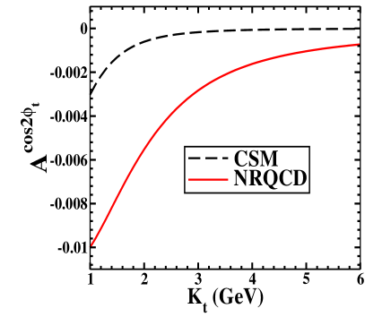
(a)   (b)

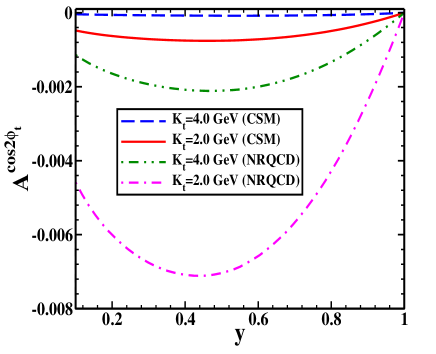
(c)

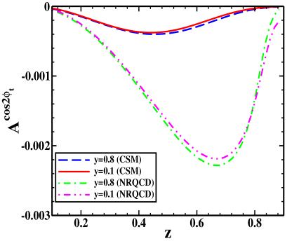
Figure 3: $\cos 2\phi_{t}$ asymmetry calculated in TMD evolution approach for $e+p\rightarrow e+J/\psi+Jet+X$, in both NRQCD and in the CS; as functions of (a) $\mathrm{K}_{t}$, (b) $y$ and (c) $z$. We have used $\sqrt{s}=140\leavevmode\nobreak\$GeV. In (a) and (b) we have used $z=0.7$. In (a) we have taken $0.1\leq y\leq 1$ for the range of $y$ integration and in (b) we have used fixed values of $\mathrm{K}_{t}$. In (c) we have taken $\mathrm{K}_{t}=3\leavevmode\nobreak\$GeV and fixed values of $y$. We have used CMSWZ set of LDMEs Chao et al. (2012).

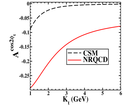
(a)   (b)

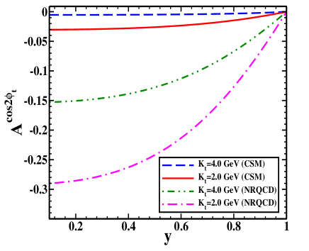
(c)

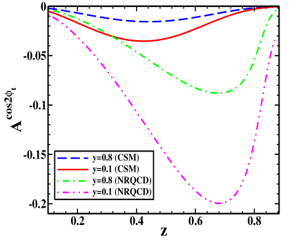
Figure 4: $\cos 2\phi_{t}$ asymmetry calculated in the spectator model for $e+p\rightarrow e+J/\psi+Jet+X$ process, in both NRQCD and in the CS; as functions of (a) $\mathrm{K}_{t}$, (b) $y$ and (c) $z$. We have used $\sqrt{s}=140$ GeV. In (a) and (b) we have used $z=0.7$. In (a) we have taken $0.1\leq y\leq 1$ for the range of $y$ integration and in (b) we have used fixed values of $\mathrm{K}_{t}$. In (c) we have taken $\mathrm{K}_{t}=3\leavevmode\nobreak\$GeV and fixed values of $y$. We have used CMSWZ set of LDMEs Chao et al. (2012).

In the upper left panel (a) of Figs. 3-5, we have plotted the $\cos 2\phi_{t}$ asymmetry as functions of $\mathrm{K}_{t}$ at $\sqrt{s}=140\leavevmode\nobreak\$GeV. In these plots, we integrated $\mathrm{q}_{t}$ and $y$ in the range $(0,1)$ and, $(0.1,1)$ respectively. We see that the $\cos 2\phi_{t}$ asymmetry is maximum (negative) for lower $\mathrm{K}_{t}$ and monotonically decreases as we go in the higher $\mathrm{K}_{t}$ region. The maximum asymmetry we obtained is $\approx 29\%$ in the spectator model at $\mathrm{K}_{t}=1\leavevmode\nobreak\$GeV followed by the Gaussian parameterization, $\approx 17\%$. Incorporation of the TMD evolution results in a smaller asymmetry, $\approx 1\%$ at $\mathrm{K}_{t}=1$ GeV.

The $y$ dependence of $\cos 2\phi_{t}$ azimuthal asymmetry is shown in the upper right panel (b) of Figs. 3-5 at $\sqrt{s}=140\leavevmode\nobreak\$GeV; we have shown the results both in NRQCD and in the CS. We plotted the asymmetry for two fixed values of $\mathrm{K}_{t}$, namely $2\leavevmode\nobreak\$GeV and $4\leavevmode\nobreak\$GeV. We have plotted the asymmetry in the range of $y\in[0.1,1]$, however in the lower $y$ region, the magnitude of the asymmetry is similar in both the spectator and the Gaussian models, whereas in TMD evolution approach, the asymmetry is maximum around $y=0.44$ at $\mathrm{K}_{t}=2\leavevmode\nobreak\$GeV in NRQCD. The asymmetry is small in the TMD evolution approach; however, we obtain a significant asymmetry, $\approx 29\%$, in the spectator model followed with $\approx 18\%$ in the Gaussian model at $\mathrm{K}_{t}=2\leavevmode\nobreak\$GeV and $y=0.1$.

In all the above discussed plots of the asymmetry as functions of $\mathrm{K}_{t}$ and $y$, we have taken a fixed value of $z=0.7$. However, in the lower panel (c) of Figs. 3-5, we have plotted the $\cos(2\phi_{t})$ asymmetry as functions of $z$ at $\sqrt{s}=140\leavevmode\nobreak\$GeV and $\mathrm{K}_{t}=3\leavevmode\nobreak\$GeV for both NRQCD and the CS. We have taken fixed values of $y$, namely, $0.1$ and $0.8$. The peak of the asymmetry is $\approx 12\%$ at $z\approx 0.7$ in NRQCD and $\approx 2\%$ at $z\approx 0.4$ in the CS at $y=0.1$. In all these plots, we have used LDMEs from Chao et al. (2012).

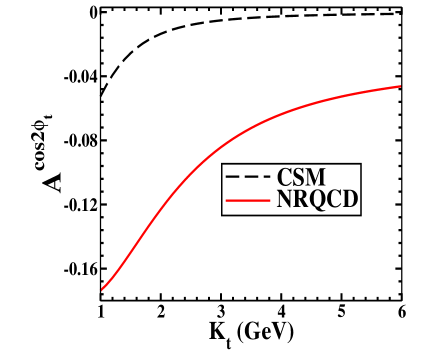
(a)   (b)

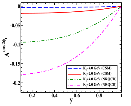
(c)

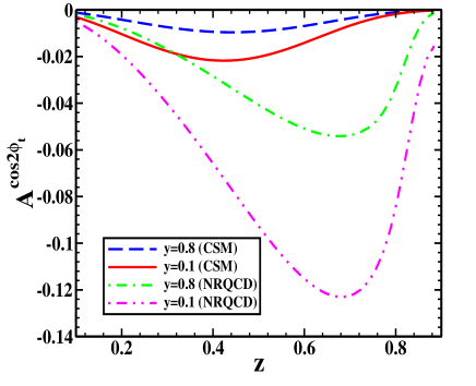
Figure 5: $\cos 2\phi_{t}$ asymmetry calculated using Gaussian parameterization of TMDs for $e+p\rightarrow e+J/\psi+Jet+X$ process, as functions of (a) $\mathrm{K}_{t}$, (b) $y$ and (c) $z$. We have used $\sqrt{s}=140\leavevmode\nobreak\$GeV. In (a) and (b) we have used $z=0.7$. In (a) we have taken $0.1\leq y\leq 1$ for the range of $y$ integration and in (b) we have used fixed values of $\mathrm{K}_{t}$. In (c) we have taken $\mathrm{K}_{t}=3\leavevmode\nobreak\$GeV and fixed values of $y$. We have used CMSWZ set of LDMEs Chao et al. (2012).

In Fig. 6, we have plotted both the TMDs, $f_{1}^{g}$ and $h_{1}^{\perp g}$ and their ratio, $\frac{\mathrm{q}_{t}^{2}h_{1}^{\perp g}}{2M_{P}^{2}f_{1}^{g}}$ as functions of $\mathrm{q}_{t}$ for all three parameterizations. In all these plots we have used similar kinematics as we considered for the plots in Fig. 3-7. In this kinematics, the $x$ value of the gluon TMDs are of the order of $10^{-3}-10^{-2}$. We have plotted at the probing scale which is the virtuality of photon, $Q^{2}=M_{\psi}^{2}+\mathrm{K}_{t}^{2}$, where $\mathrm{K}_{t}=3$ GeV and at the fixed values of $y=0.3$ and $z=0.7$. This sets $x\approx 0.012$. From the plots of the ratio, $\frac{\mathrm{q}_{t}^{2}h_{1}^{\perp g}}{2M_{P}f_{1}^{g}}$ ((d) of Fig. 6), we see that the TMDs in the spectator model indeed saturates the positivity bound, whereas, the Gaussian parameterizations and TMD evolution approach satisfy the positivity bound but do not saturate it except for $\mathrm{q}_{t}\approx 0.36$ GeV, where Gaussian parameterization is saturating the positivity bound. Moreover, the ratio is larger in the case of Gaussian as compared with TMD evolution approach for almost whole range of $\mathrm{q}_{t}$ considered. In the Spectator model, tails of the TMDs in the small-$x$ domain, depend on the trend of spectral function at large $M_{X}$ Bacchetta et al. (2020, 2020). We have checked that the spectator model results in Eqs. (12) and (15) of Bacchetta et al. (2020) for the ratio $\frac{\mathrm{q}_{t}^{2}h_{1}^{\perp g}}{2M_{P}^{2}f_{1}^{g}}$ at $x=0.001$ without integrating over the spectral function, does not saturate the positivity bound when $M_{X}$ is large. However, if we multiply by the spectral function and integrate over $M_{X}$, the TMDs saturate the positivity bound when $x$ is of the order of $10^{-3}-10^{-2}$; this could be because the spectral function is zero for higher values of $M_{X}$ in replica 11. However, in the higher $x$ region, the TMDs do not saturate the bound but satisfies it for the whole range of the transverse momentum, $\mathrm{q}_{t}$.

In Fig. 7, we show a comparison of the upper bound of the asymmetry with that calculated in Spectator model, Gaussian model and TMD evolution approach at $\sqrt{s}=140$ GeV. The upper bound of the asymmetry is calculated by saturating the positivity bound of TMDs in Eq. (78) and fixing all the parameters mentioned above. We have shown the result both in NRQCD and CS as a function of $\mathrm{K}_{t}$ at $y=0.3$ (upper panel) and as a function of $y$ at $\mathrm{K}_{t}=2$ GeV in the lower panel. In case of TMD evolution, the non - perturbative Sudakov factor corresponding to $\mathrm{b}_{tlim}=2\leavevmode\nobreak\ \mathrm{GeV}^{-1}$. For all the plots the range of integration of $\mathrm{q}_{t}\in[0.0-1.0]\mathrm{GeV}$, $z=0.7$ and we have fixed the virtuality of photon $Q=\sqrt{M_{\psi}^{2}+\mathrm{K}_{t}^{2}}$.

We can see that the asymmetry calculated with the spectator model is maximum and agrees with the upper bound. As seen from Fig. 7, the asymmetry incorporating TMD evolution is significantly smaller than that calculated using Gaussian and spectator models for the gluon TMDs. This is because the denominator of the asymmetry receives contribution from the unpolarized gluon distribution which has a leading order (LO) term Eq. (61) whereas the numerator contains the linearly polarized gluon distribution whose leading contribution comes at $O(\alpha_{s})$. If we exclude the LO term in the unpolarized gluon TMD, we find the asymmetry increases approximately three times. We also find that the magnitude of the asymmetry does not change much if $\sqrt{s}$ is lower.

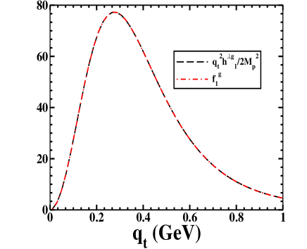
(a)   (b)

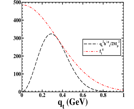
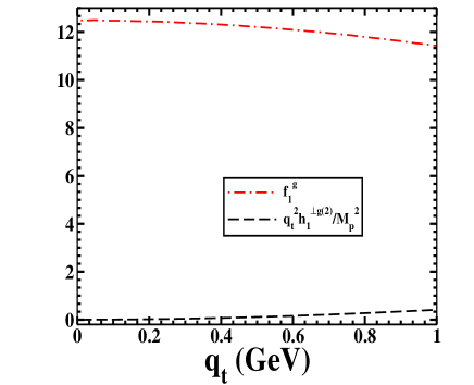
(c)   (d)

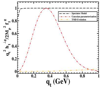
Figure 6: Unpolarized and linearly polarized gluon TMDs as a function of $\mathrm{q}_{t}$ calculated in spectator model (a), Gaussian model (b) and TMD evolution (c), respectively at $\sqrt{s}=140$, $\mathrm{K}_{t}=3.0\mathrm{GeV}$, $y=0.3$ and $z=0.7$. (d) panel shows the comparison between the positivity bound for all the parameterizations.

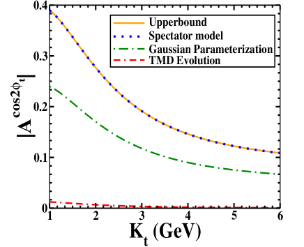
(a)   (b)

(c)   (d)

Figure 7: Upper bound of the asymmetry compared with the absolute values of $A^{\cos 2\phi_{t}}$ calculated in spectator model, Gaussian model and TMD evolution, respectively, for $e^{-}+P\to e^{-}+J/\psi+Jet+X$ at $\sqrt{s}=140$. Left panel shows the asymmetry in NRQCD and right panel in CS. We have taken $y=0.3$ in the upper panel ((a) and (b)) and $\mathrm{K}_{t}=2$ GeV in the lower panel ((c) and (d)).

Lastly, in Fig. 8, we show the upper bound for the absolute value of $|A^{\cos 2\phi_{t}}|$ within the NRQCD using two sets of LDMEs, as well as the contributions coming from individual states $i.e.$, ${}^{1}S_{0}^{(8)},^{3}S_{1}^{(1,8)}$ and ${}^{3}P_{j}^{(8)}$. One can see from (a) that for the LDME set CMSWZ Chao et al. (2012), the dominating contribution comes from one single state, ${}^{1}S_{0}^{(8)}$; while from (b) one can see that for SV set of LDME Sharma and Vitev (2013), the dominating contribution comes from two states, ${}^{1}S_{0}^{(8)}$ and ${}^{3}P_{j}^{(8)}$. So, we can conclude that the asymmetry depends on the LDME set chosen. It is worth mentioning here that our results for the upper bound of the asymmetry do not match with those presented in D’Alesio et al. (2019) even if we plot it using the same scale as in this reference. We have traced this mismatch to a difference in the sign of the contribution coming from the ${}^{3}P_{0}^{(8)}$ state to the coefficient $\mathbb{B}_{0}$.

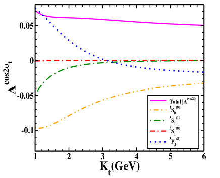
Figure 8: Contribution to the upper bound of the asymmetry coming from individual states, as a function of $\mathrm{K}_{t}$ at $\sqrt{s}=140$ GeV, $Q=\sqrt{M_{\psi}^{2}+\mathrm{K}_{t}^{2}}$ and $y=0.3$; (a) using the CMSWZ set of LDMEs Chao et al. (2012) and (b) using the SV set of LDMEs Sharma and Vitev (2013)

VII Conclusion

We have presented a calculation of the $\cos 2\phi_{t}$ asymmetry in almost back-to-back production of a $J/\psi$ and a jet in $ep$ collision, using TMD factorization and generalized parton model. This asymmetry is sensitive to the still unknown linearly polarized gluon distribution. We present a numerical estimate of the asymmetry in the kinematical region that will be accessible at the future EIC. We have used NRQCD to calculate the $J/\psi$ production rate and two recent parameterization for the gluon TMDs, one based on a Gaussian type distribution and another based on spectator model. The asymmetry is quite sizable; in fact in spectator model the asymmetry agrees with the upper bound that is obtained by saturating the positivity condition of the gluon TMDs. TMD evolution affects the asymmetry at the energy of the EIC, making it smaller. The asymmetry also depends on the LDMEs used, and dominating contribution comes from different states. We conclude that the back-to-back production of $J/\psi$ and a jet at the future EIC will be a very useful channel to probe the linearly polarized gluon TMDs.

VIII Acknowledgement

We acknowledge the funding from Board of Research in Nuclear Sciences (BRNS), Govt. of India, under sanction No. 57/14/04/2021-BRNS/57082. We thank A. Bacchetta, M. Radici and F. Celiberto for useful discussion.

References

- Mulders and Tangerman (1996) P. J. Mulders and R. D. Tangerman, Nucl. Phys. B 461, 197 (1996), [Erratum: Nucl.Phys.B 484, 538–540 (1997)], eprint hep-ph/9510301.
- Boer and Mulders (1998) D. Boer and P. Mulders, Physical Review D 57, 5780 (1998).
- Boer et al. (2000) D. Boer, R. Jakob, and P. Mulders, Nuclear Physics B 564, 471 (2000).
- Anselmino et al. (1999) M. Anselmino, M. Boglione, and F. Murgia, Physical review D 60, 054027 (1999).
- Anselmino et al. (1995) M. Anselmino, M. Boglione, and F. Murgia, Physics letters B 362, 164 (1995).
- Barone et al. (2002) V. Barone, A. Drago, and P. G. Ratcliffe, Physics reports 359, 1 (2002).
- Collins (2011) J. Collins, Foundations of perturbative QCD, vol. 32 (Cambridge University Press, 2011).
- Echevarria et al. (2012) M. G. Echevarria, A. Idilbi, and I. Scimemi, JHEP 07, 002 (2012), eprint 1111.4996.
- Echevarría et al. (2013) M. G. Echevarría, A. Idilbi, and I. Scimemi, Physics Letters B 726, 795 (2013).
- Echevarria (2019) M. G. Echevarria, JHEP 10, 144 (2019), eprint 1907.06494.
- Bacchetta et al. (2008) A. Bacchetta, D. Boer, M. Diehl, and P. J. Mulders, JHEP 08, 023 (2008), eprint 0803.0227.
- Fleming et al. (2020) S. Fleming, Y. Makris, and T. Mehen, JHEP 04, 122 (2020), eprint 1910.03586.
- Collins (2002) J. C. Collins, Physics Letters B 536, 43 (2002).
- Ji and Yuan (2002) X. Ji and F. Yuan, Physics Letters B 543, 66 (2002).
- Belitsky et al. (2003) A. V. Belitsky, X. Ji, and F. Yuan, Nuclear Physics B 656, 165 (2003).
- Boer et al. (2003) D. Boer, P. Mulders, and F. Pijlman, Nuclear Physics B 667, 201 (2003).
- Anselmino et al. (2017) M. Anselmino, M. Boglione, U. D’Alesio, F. Murgia, and A. Prokudin, JHEP 04, 046 (2017), eprint 1612.06413.
- Mulders and Rodrigues (2001) P. Mulders and J. Rodrigues, Physical Review D 63, 094021 (2001).
- Lansberg et al. (2018) J.-P. Lansberg, C. Pisano, F. Scarpa, and M. Schlegel, Physics Letters B 784, 217 (2018).
- Buffing et al. (2013) M. Buffing, A. Mukherjee, and P. Mulders, Physical Review D 88, 054027 (2013).
- Kovchegov and Mueller (1998) Y. V. Kovchegov and A. H. Mueller, Nuclear Physics B 529, 451 (1998).
- McLerran and Venugopalan (1999) L. McLerran and R. Venugopalan, Physical Review D 59, 094002 (1999).
- Dominguez et al. (2012) F. Dominguez, J.-W. Qiu, B.-W. Xiao, and F. Yuan, Physical Review D 85, 045003 (2012).
- Meissner et al. (2007) S. Meissner, A. Metz, and K. Goeke, Physical Review D 76, 034002 (2007).
- Marquet et al. (2018) C. Marquet, C. Roiesnel, and P. Taels, Phys. Rev. D 97, 014004 (2018), eprint 1710.05698.
- Pisano et al. (2013) C. Pisano, D. Boer, S. J. Brodsky, M. G. A. Buffing, and P. J. Mulders, JHEP 10, 024 (2013), eprint 1307.3417.
- Boer et al. (2009) D. Boer, P. J. Mulders, and C. Pisano, Physical Review D 80, 094017 (2009).
- Efremov et al. (2018a) A. Efremov, N. Y. Ivanov, and O. Teryaev, Physics Letters B 777, 435 (2018a).
- Efremov et al. (2018b) A. Efremov, N. Y. Ivanov, and O. Teryaev, Physics Letters B 780, 303 (2018b).
- Lansberg et al. (2017) J.-P. Lansberg, C. Pisano, and M. Schlegel, Nuclear Physics B 920, 192 (2017).
- Dumitru et al. (2019) A. Dumitru, V. Skokov, and T. Ullrich, Physical Review C 99, 015204 (2019).
- Sun et al. (2011) P. Sun, B.-W. Xiao, and F. Yuan, Physical Review D 84, 094005 (2011).
- Boer et al. (2013) D. Boer, W. J. Den Dunnen, C. Pisano, and M. Schlegel, Physical Review Letters 111, 032002 (2013).
- Boer et al. (2012) D. Boer, W. J. den Dunnen, C. Pisano, M. Schlegel, and W. Vogelsang, Physical review letters 108, 032002 (2012).
- Echevarria et al. (2015) M. G. Echevarria, T. Kasemets, P. J. Mulders, and C. Pisano, JHEP 07, 158 (2015), [Erratum: JHEP 05, 073 (2017)], eprint 1502.05354.
- Boer and Pisano (2012a) D. Boer and C. Pisano, Physical Review D 86, 094007 (2012a).
- Mukherjee and Rajesh (2017a) A. Mukherjee and S. Rajesh, Physical Review D 95, 034039 (2017a).
- Mukherjee and Rajesh (2016) A. Mukherjee and S. Rajesh, Physical Review D 93, 054018 (2016).
- Rajesh et al. (2021) S. Rajesh, U. D’Alesio, A. Mukherjee, F. Murgia, and C. Pisano, in 28th International Workshop on Deep Inelastic Scattering and Related Subjects (2021), eprint 2108.04866.
- Mukherjee and Rajesh (2017b) A. Mukherjee and S. Rajesh, The European Physical Journal C 77, 1 (2017b).
- Kishore and Mukherjee (2019) R. Kishore and A. Mukherjee, Physical Review D 99, 054012 (2019).
- D’Alesio et al. (2019) U. D’Alesio, F. Murgia, C. Pisano, and P. Taels, Phys. Rev. D 100, 094016 (2019), eprint 1908.00446.
- Kishore et al. (2020) R. Kishore, A. Mukherjee, and S. Rajesh, Phys. Rev. D 101, 054003 (2020), eprint 1908.03698.
- Hägler et al. (2001) P. Hägler, R. Kirschner, A. Schäfer, L. Szymanowski, and O. Teryaev, Physical Review Letters 86, 1446 (2001).
- Yuan and Chao (2001) F. Yuan and K.-T. Chao, Physical Review Letters 87, 022002 (2001).
- Yuan (2008) F. Yuan, Physical Review D 78, 014024 (2008).
- Bodwin et al. (1995) G. T. Bodwin, E. Braaten, and G. P. Lepage, Phys. Rev. D 51, 1125 (1995), [Erratum: Phys.Rev.D 55, 5853 (1997)], eprint hep-ph/9407339.
- Boer et al. (2021) D. Boer, C. Pisano, and P. Taels, Phys. Rev. D 103, 074012 (2021), eprint 2102.00003.
- Lepage et al. (1992) G. P. Lepage, L. Magnea, C. Nakhleh, U. Magnea, and K. Hornbostel, Physical Review D 46, 4052 (1992).
- Berger and Jones (1981) E. L. Berger and D. Jones, Physical Review D 23, 1521 (1981).
- Baier and Rückl (1983) R. Baier and R. Rückl, Zeitschrift für Physik C Particles and Fields 19, 251 (1983).
- Rajesh et al. (2018a) S. Rajesh, R. Kishore, and A. Mukherjee, Phys. Rev. D 98, 014007 (2018a), URL https://link.aps.org/doi/10.1103/PhysRevD.98.014007.
- Boer and Pisano (2012b) D. Boer and C. Pisano, Phys. Rev. D 86, 094007 (2012b), URL https://link.aps.org/doi/10.1103/PhysRevD.86.094007.
- Sharma and Vitev (2013) R. Sharma and I. Vitev, Phys. Rev. C 87, 044905 (2013), URL https://link.aps.org/doi/10.1103/PhysRevC.87.044905.
- Chao et al. (2012) K.-T. Chao, Y.-Q. Ma, H.-S. Shao, K. Wang, and Y.-J. Zhang, Phys. Rev. Lett. 108, 242004 (2012), URL https://link.aps.org/doi/10.1103/PhysRevLett.108.242004.
- Rajesh et al. (2018b) S. Rajesh, R. Kishore, and A. Mukherjee, Physical Review D 98, 014007 (2018b).
- Graudenz (1994) D. Graudenz, Physical Review D 49, 3291 (1994).
- Aybat and Rogers (2011a) S. M. Aybat and T. C. Rogers, Phys. Rev. D 83, 114042 (2011a), eprint 1101.5057.
- Aybat et al. (2012a) S. M. Aybat, A. Prokudin, and T. C. Rogers, Phys. Rev. Lett. 108, 242003 (2012a), eprint 1112.4423.
- Echevarria et al. (2014a) M. G. Echevarria, A. Idilbi, Z.-B. Kang, and I. Vitev, Physical Review D 89, 074013 (2014a).
- Aybat et al. (2012b) S. M. Aybat, J. C. Collins, J.-W. Qiu, and T. C. Rogers, Physical Review D 85, 034043 (2012b).
- Echevarria et al. (2014b) M. G. Echevarria, A. Idilbi, and I. Scimemi, Physical review D 90, 014003 (2014b).
- Boer et al. (2020) D. Boer, U. D’Alesio, F. Murgia, C. Pisano, and P. Taels, Journal of High Energy Physics 2020, 1 (2020).
- Tangerman and Mulders (1995) R. Tangerman and P. Mulders, Physical Review D 51, 3357 (1995).
- van Daal (2016) T. van Daal, arXiv preprint arXiv:1612.06585 (2016).
- Kovchegov and Levin (2012) Y. V. Kovchegov and E. Levin, Quantum chromodynamics at high energy (Cambridge University Press, 2012).
- Scarpa et al. (2020) F. Scarpa, D. Boer, M. G. Echevarria, J.-P. Lansberg, C. Pisano, and M. Schlegel, The European Physical Journal C 80, 1 (2020).
- Landry et al. (2003) F. Landry, R. Brock, P. M. Nadolsky, and C.-P. Yuan, Phys. Rev. D 67, 073016 (2003), URL https://link.aps.org/doi/10.1103/PhysRevD.67.073016.
- Aybat and Rogers (2011b) S. M. Aybat and T. C. Rogers, Phys. Rev. D 83, 114042 (2011b), URL https://link.aps.org/doi/10.1103/PhysRevD.83.114042.
- Bacchetta et al. (2020) A. Bacchetta, F. G. Celiberto, M. Radici, and P. Taels, Eur. Phys. J. C 80, 733 (2020), eprint 2005.02288.
- Martin et al. (2009) A. D. Martin, W. J. Stirling, R. S. Thorne, and G. Watt, The European Physical Journal C 63, 189 (2009).
- Shtabovenko et al. (2020) V. Shtabovenko, R. Mertig, and F. Orellana, arXiv preprint arXiv:2001.04407 (2020).
- Mertig et al. (1991) R. Mertig, M. Böhm, and A. Denner, Computer Physics Communications 64, 345 (1991).