Efficient $k$-clique Listing with Set Intersection Speedup

Abstract

Listing all $k$-cliques is a fundamental problem in graph mining, with applications in finance, biology, and social network analysis. However, owing to the exponential growth of the search space as $k$ increases, listing all $k$-cliques is algorithmically challenging. DDegree and DDegCol are the state-of-the-art algorithms that exploit ordering heuristics based on degree ordering and color ordering, respectively. Both DDegree and DDegCol induce high time and space overhead for set intersections cause they construct and maintain all induced subgraphs. Meanwhile, it is non-trivial to implement the data level parallelism to further accelerate on DDegree and DDegCol.

In this paper, we propose two efficient algorithms SDegree and BitCol for $k$-clique listing. We mainly focus on accelerating the set intersections for $k$-clique listing. Both SDegree and BitCol exploit the data level parallelism for further acceleration with single instruction multiple data (SIMD) or vector instruction sets. Furthermore, we propose two preprocessing techniques Pre-Core and Pre-List, which run in linear time. The preprocessing techniques significantly reduce the size of the original graph and prevent exploring a large number of invalid nodes. In the theoretical analysis, our algorithms have a comparable time complexity and a slightly lower space complexity than the state-of-the-art algorithms. The comprehensive experiments reveal that our algorithms outperform the state-of-the-art algorithms by $3.75$x for degree ordering and $5.67x$ for color ordering on average.

I Introduction

Real-world graphs, such as social networks, road networks, world-wide-web networks, and IoT networks often consist of cohesive subgraph structures. Cohesive subgraph mining is a fundamental problem in network analysis, with applications in community detection [1, 2, 3, 4, 5], real-time story identification [6], frequent migration patterns mining in financial markets [7], and motif detection in biological networks [8].

Clique is a cohesive subgraph structure par excellence with a variety of applications in network analysis [9, 10, 11]. A $k$-clique is a dense subgraph of a graph $G$ with $k$ nodes, and each pair of nodes are adjacent [12]. The $k$-clique listing problem is a natural generalization of the triangle listing problem [13]. In particular, the state-of-the-art triangle listing algorithm [14] is capable of processing billion-scale graphs within $1,000$ seconds. However, the $k$-clique listing problem is often deemed not feasible even for million-scale graphs, since the number of $k$-cliques could be exponentially large for a relatively large $k$ [15, 12].

Applications. In recent years, the requirement of efficiently listing $k$-cliques has been raised by the data mining and database communities. We introduce the applications of $k$-clique listing as follows.

(1) Community Detection. Detecting communities helps to reveal the structural organizations in real-world complex networks [16]. Specifically, a $k$-clique community is the union of all the $k$-cliques that each $k$-clique is adjacent to another one [16, 17]. Hui and Crowcroft [18] designed efficient forwarding algorithms for mobile networks with information in $k$-clique communities. The $k$-clique listing algorithms can be exploited to compute $k$-clique communities [16, 17].

(2) Spam Detection. Link spam is an attempt to promote the ranking of websites by cheating the link-based ranking algorithm in search engines [19]. Clique identification in the network structure helps a lot in handling the search engine spam problems, especially the link spam [20]. In particular, Jayanthi et al. [20] proposed a $k$-clique percolation method to detect the spam, which also needs to list the $k$-cliques.

(3) Biological Networks. Most cellular tasks are not performed by individual proteins, but by a group of functionally related proteins (often called modules). In gene association networks, Adamcsek et al. [21] proposed CFinder to predict the function of a single protein and to discover novel modules. CFinder needs to locate the $k$-clique percolation clusters of the network interpreted as modules, in which a $k$-clique listing algorithm can be used for computing all $k$-cliques.

Motivated by the aforementioned studies, we investigate the problem of listing all the $k$-cliques in a graph. A $k$-clique can be expanded from a ($k$-$1$)-clique. Therefore, a basic idea of the $k$-clique listing algorithms is to recursively expand the clique, starting from a single node ($1$-clique).

Existing Works. Based on a recursive framework, numerous practical algorithms have been developed for listing all the $k$-cliques in real-world graphs [22, 15, 12].

The state-of-the-art algorithms [15, 12] are based on vertex ordering and mainly focus on the construction of each induced subgraph in the recursion. Danisch et al. [12] proposed an efficient ordering-based framework kClist for listing all the $k$-cliques, which can be easily parallelized. Li et al. [15] extended kClist by proposing a new color ordering heuristics based on greedy graph coloring [23], which can prune more unpromising search paths.

To the best of our knowledge, all the state-of-the-art algorithms focus on selecting appropriate vertex ordering strategies to improve the theoretical upper bound of the time complexity.

Our Approaches. Existing algorithms [22, 15, 12] are implemented efficiently with well-designed hash tables. Furthermore, reordering nodes in the adjacency lists is sufficient for constructing the induced subgraphs, without generating a completely new one. Our approaches achieve even better performance with merge join, avoiding careful maintenance of induced subgraphs.

In this paper, we focus on accelerating the set intersections in each recursion, thereby accelerating the $k$-clique listing. Our algorithms are implemented based on the merge join, without additional operations on reordering nodes or recursively maintaining hash tables.

Our algorithms exploit the data level parallelism, e.g., single instruction multiple data (SIMD) and vector instruction sets [24, 25], to further accelerate the set intersections [26, 27, 28]. We have to emphasize that, the state-of-the-art algorithms are based on hash join with the reordered nodes in each recursion, which is non-trivial to exploit the data level parallelism.

Contributions. Our contributions in this paper are summarized as follows:

• Pre-Core and Pre-List. We develop two preprocessing algorithms, named Pre-Core and Pre-List, that not only significantly reduce the search space of the original graph, but also finish in satisfactory time.

• SDegree and BitCol. We propose a simple but effective merge-based algorithm SDegree for listing all the $k$-cliques, without reordering nodes or maintaining hash tables. BitCol improves SDegree by exploiting the color ordering and compressing the vertex set with a binary representation to compare more elements at a time. Both SDegree and BitCol are compatible with the data level parallelism to further accelerate the $k$-clique listing, which is non-trivial for hash-based algorithms.

• Efficiency. Our algorithms are efficient both theoretically and experimentally. On one hand, we achieve the same upper bound on the time complexity with less memory overhead compared to the state-of-the-art algorithms. On the other hand, we evaluate the serial and the parallel version of our algorithms on $10$ real-world datasets. Our algorithms outperform the state-of-the-art algorithms by $3.75$x for degree ordering and $5.67x$ for color ordering on average.

Paper Organization. The rest of the paper is organized as follows. Section II surveys the important related works. Section III gives a formal definition of the problem and related concepts, and briefly introduces the existing solutions. Section IV presents the overall framework briefly. The preprocessing techniques are proposed in Section V. Our algorithms are formally introduced in Section VI and Section VII. The theoretical analysis is given in Section VIII. Then the extensive experiments are conducted in Section IX. Finally, Section X concludes the paper.

II Related Work

II-A The Bron-Kerbosch Algorithm

Relying on the fact that each $n$-clique ($n\geq k$) consists of $\tbinom{n}{k}$ $k$-cliques, the algorithms for maximal clique enumerating (MCE) can be applied to the problem of $k$-clique listing. The classic Bron-Kerbosch algorithm [29] solves the MCE problem by recursively maintaining the processed states of three sets $R$, $P$, $X$, to search the maximal cliques without redundant verification. $R$ stands for the currently acquired growing clique; $P$ stands for prospective nodes that may be adjacent to each node in $R$, with which $R$ can be further expanded; $X$ stands for the nodes already processed. Initially, $P=V$, $R=\emptyset$, and $X=\emptyset$. After exploring the vertex $v$, $v$ is transferred from $P$ to $X$. The Bron-Kerbosch algorithm avoids reporting the maximal clique repeatedly by checking $X$. Specifically, a maximal clique is reported only when $P=\emptyset$ and $X=\emptyset$, since no more elements can be added to $R$.

Furthermore, Bron and Kerbosch proposed a variant version with a pivoting strategy, which reduces the number of unnecessary recursive calls. Eppstein et al. [30] improved the original Bron-Kerbosch algorithm with vertex ordering, which reduces the exponential worst-case time complexity.

II-B Vertex Ordering Approach

A common strategy to avoid redundancy and reduce the search space is the vertex ordering, which is a preprocessing step that transforms the original undirected graph into a directed acyclic graph (DAG). The orientation of each undirected edge is from the low order to the high order. Initially, vertex ordering is a classical technique designed for the triangle listing problem. It is capable of accelerating the calculation both theoretically and experimentally, by properly selecting the orientation of each edge [14]. Therefore, it is critical in determining the appropriate order of each vertex.

In recent years, vertex ordering has been successfully applied to the $k$-clique listing problem with good performance [15, 12]. The correctness is based on the fact that the $k$-clique can be discovered in any order, for the symmetrical structure of the clique. Common vertex ordering approaches include degeneracy ordering [12, 30], degree ordering [14, 13, 15], and color ordering [15].

The degeneracy ordering can be generated by the classic core-decomposition algorithm [31], which repeatedly deletes the node with the minimum degree. The degree ordering is simply generated by the degree of each vertex in descending order. The color ordering is based on the greedy graph coloring [23], which assigns each vertex a color value such that no adjacent vertices share the same color. In particular, the out-degree in the DAG based on degeneracy ordering is bounded by the degeneracy ($\beta$) [12], while the out-degree is bounded by the $h$-index ($\gamma$) for degree ordering [15].

II-C Set Intersection Acceleration

As reported in  [28, 32], the set intersection is extensively involved in graph algorithms, such as triangle listing and maximal clique enumeration. Similarly, the $k$-clique listing problem also involves a large number of set intersections, which certainly causes a bottleneck.

Given two vertex sets $S_{a}$ and $S_{b}$, there are four major methods for set intersections. Hash join has a time complexity of $O(|S_{a}|)$ with $S_{b}$ as the hash table. The additional cost is required to construct and maintain the hash tables. If $S_{a}$ and $S_{b}$ are sorted in ascending order, we can use merge-based algorithms and galloping search for set intersections [33, 34]. The time complexity of the merge-based algorithm is $O(|S_{a}|)$ (or $O(|S_{b}|)$) in the best case while $O(|S_{a}|+|S_{b}|)$ in the worst case; the time complexity of the galloping search is $O(|S_{a}|\log{|S_{b}|})$, which is efficient in practice only for $|S_{a}|\ll|S_{b}|$.

Modern microprocessors are equipped with SIMD or vector instruction sets which allow compilers to exploit fine-grained data level parallelism [24]. The application of SIMD instructions to accelerate set intersections is proposed by a bunch of algorithms [26, 35, 28]. With SIMD instructions, the merge-based algorithm can be extended by reading and comparing multiple elements at a time. In particular, the state-of-the-art algorithms for accelerating the set intersections [32, 28] are mostly developed based on merge join, instead of hash join or galloping search.

III Preliminary

The formal definition of the $k$-clique listing problem is given in this section. The existing algorithms, Chiba-Nishizeki [22], kClist [12], DDegree and DDegCol [15], are then introduced. TABLE I summarizes the most relevant notations.

TABLE I: Notations

Notations	Description
$G,\mathop{G}\limits^{\rightarrow}$	Undirected graph, directed graph
$V$, $E$	Graph vertex set, edge set
$N_{v},d_{v}$	The neighbor set of $v\in G$ and its size
$N^{+}_{v},d^{+}_{v}$	The out neighbors of $v\in\mathop{G}\limits^{\rightarrow}$ and its size
$G_{u}$	The subgraph induced by the neighbors of $u$ in $G$
$\Omega_{k},C_{k}$	$k$-core, $k$-clique
$\Delta$	The maximum out-degree in $\mathop{G}\limits^{\rightarrow}$

III-A Problem Definition

$G(V,E)$ is an undirected and unlabeled graph, where $V$ ($|V|=n$) and $E$ ($|E|=m$) denote the set of nodes and the set of edges, respectively. The neighbor set of $v$ in $G$ is denoted by $N_{v}(G)$, and the degree of $v$ in $G$ is denoted by $d_{v}(G)=|N_{v}(G)|$. We use $N_{v}$ and $d_{v}$ to refer to $N_{v}(G)$ and $d_{v}(G)$ when the context is clear. If $V^{\prime}\subseteq V$ and $E^{\prime}=\{(u,v)|(u,v)\in E,u\in V^{\prime}\land v\in V^{\prime}\}$, a subgraph $G^{\prime}(V^{\prime},E^{\prime})$ is termed an induced subgraph of $G$.

Definition 1 ($k$-core).

Given a graph $G(V,E)$, an induced subgraph $\Omega_{k}(V_{H},E_{H})$ is a $k$-core of $G$, if $\Omega_{k}$ satisfies the following constraints:

1. Cohesive: For any $u\in V_{H}$, $d_{u}\geq k$.

2. Maximal: $H$ is maximal, i.e., for any vertex set $H^{\prime}\supset H$, the subgraph induced by $H^{\prime}$ is not a $k$-core.

Definition 2 ($k$-clique).

A $k$-clique $C_{k}(V_{k},E_{k})$ is an induced subgraph of $G$ where $|V_{k}|=k$ and $|E_{k}|=\tbinom{k}{2}$, i.e., every two nodes are adjacent in $C_{k}$.

The $k$-clique listing problem is to find all the $k$-cliques in $G$, which is a natural generalization of the triangle listing problem [14, 13]. Since a $2$-clique is an edge, we only consider $k\geq 3$ by default in this paper.

Example 1.

The graph $G$ in Fig.1 has three $4$-cliques $\{v_{9},v_{10},v_{11},v_{12}\},\{v_{1},v_{2},v_{3},v_{4}\},$ and $\{v_{1},v_{2},v_{4},v_{6}\}$.

Figure 1: The Input Graph $G$

We use $\mathop{G}\limits^{\rightarrow}$ to denote a directed graph. The set of directed edges $\{\langle u,v\rangle\}$ in $\mathop{G}\limits^{\rightarrow}$ is denoted as $E(\mathop{G}\limits^{\rightarrow})$, where the direction of $\langle u,v\rangle$ is $u\rightarrow v$. The set of nodes in $\mathop{G}\limits^{\rightarrow}$ is denoted as $V(\mathop{G}\limits^{\rightarrow})$. A directed acyclic graph (DAG) is a directed graph with no directed cycles. We denote with $N^{+}_{v}(\mathop{G}\limits^{\rightarrow})$ the out-neighbor set of $v$ in $\mathop{G}\limits^{\rightarrow}$, and $d^{+}_{v}(\mathop{G}\limits^{\rightarrow})=|N^{+}_{v}(\mathop{G}\limits^{\rightarrow})|$ denotes the out-degree of $v$. If the context is clear, we use $N^{+}_{v}$ and $d^{+}_{v}$ to refer to $N^{+}_{v}(\mathop{G}\limits^{\rightarrow})$ and $d^{+}_{v}(\mathop{G}\limits^{\rightarrow})$. The vertex ordering of the undirected graph $G(V,E)$ is determined by an assignment function $\eta:V\rightarrow\{1,2,\ldots,|V|\}$. An undirected edge $(u,v)$ can be converted into a directed edge $\langle u,v\rangle$ with $\eta$, where $\eta(u)<\eta(v)$. In graph $G$ of Fig.1, we utilize the node ID as $\eta$ and the directed version $\mathop{G}\limits^{\rightarrow}$ is shown in Fig.2.

Figure 2: The Directed Version of $G$

Arboricity ($\alpha$) [22, 36, 37], degeneracy ($\beta$) [30], and $h$-index ($\gamma$) [37, 38] are three important metrics in graph analysis that we will discuss.

For algorithm design and complexity analysis, these metrics are commonly utilized in the $k$-clique listing problem. In particular, $\alpha$, $\beta$ and $\gamma$ are usually very small in real-world graphs[30].

• Arboricity ($\alpha$). The arboricity of an undirected graph $G(V,E)$, i.e., $\alpha$, is the minimum number of forests into which the edges of $G$ can be partitioned. The arboricity $\alpha$ can be used to measure the density of $G$, however, it is difficult to be calculated.

• Degeneracy ($\beta$). The degeneracy, denoted as $\beta$, is the maximum core number of $G$, where the core number of a vertex $u$ is the largest integer $l$ s.t. $u$ is contained by a $l$-core. $\beta$ can be calculated in linear time with the classic core-decomposition algorithm [31]. $\beta$ is frequently utilized to approximate the arboricity $\alpha$ since $\alpha\leq\beta\leq 2\alpha$ - $1$ [15].

• $h$-index ($\gamma$). The $h$-index of $G$, denoted as $\gamma$, can be written as $\gamma=\mathop{\arg\max}\limits_{h}{(|\{v|d_{v}(G)\geq h\}|\geq h,v\in V)}$, which is the maximum $h$ such that $G$ contains $h$ vertices with a degree at least $h$ [37]. Similarly, $\gamma$ also satisfies that $\alpha\leq\gamma\leq\sqrt{m}$.

III-B Existing Solutions

III-B1 The Chiba-Nishizeki Algorithm

We start by introducing the iconic Chiba-Nishizeki algorithm [22], which is the first practical algorithm for the $k$-clique listing problem. As illustrated in Algorithm 1, the nodes are sorted by degree in descending order, i.e., $v_{i}<v_{j}$ for $d(v_{i})>d(v_{j})$ (Line 1). For each vertex $v_{i}$, the induced subgraph $G_{v_{i}}$ is constructed by the neighbors of $v_{i}$ (Line 1). Subsequently, the algorithm invokes the recursive procedure for each induced subgraph, with a recurrence depth of $k$-$1$ (Line 1). To prevent repeating computations, $v_{i}$ and its related edges are eliminated when $G_{v_{i}}$ is processed (Line 1).

The time complexity of the Chiba-Nishizeki algorithm is $O(km\alpha^{k-2})$, which is closely associated with the arboricity. In most real-world graphs, the arboricity is generally rather small. Therefore, the Chiba-Nishizeki algorithm is proved to be effective in practice. However, the parallelization of the Chiba-Nishizeki algorithm is difficult, since each vertex $v_{i}$ is eliminated after $G_{v_{i}}$ has been processed, i.e., $G$ shrinks throughout each iteration.

Input: A graph $G$ and a positive integer $k$

Output: All the $k$-cliques in $G$

1 List($G$, $\emptyset$, $k$)

2 Procedure List($G$, $R$, $l$)

3 if $l\neq 2$ then

4       Sort the nodes by degree in descending order

5       for $i=1$ to $|V(G)|$ do

6             Compute the subgraph $G_{v_{i}}$ induced by $N_{v_{i}}$

7             List($G_{v_{i}}$, $R\cup\{v_{i}\}$, $l-1$)

8             Remove $v_{i}$ and the related edges in $G$

9            

10      

11 else

12       for each edge $(u,v)\in G$ do

13             report a $k$-clique $R\cup\{u,v\}$

14            

15      

16

Algorithm 1 Chiba-Nishizeki($G$, $k$)

III-B2 kClist

Danisch et al.[12] proposed kClist for listing all the $k$-cliques using the technique of vertex ordering. Algorithm 2 delves further into the framework of the kClist algorithm. First, a total ordering $\eta$ on nodes is selected (Line 2). Based on the classic core-decomposition algorithm [31], Danisch et al. specified the degeneracy ordering as the total ordering $\eta$. kClist creates a DAG $\mathop{G}\limits^{\rightarrow}$ based on the total ordering (Line 2) and lists all the $k$-cliques on $\mathop{G}\limits^{\rightarrow}$ without redundancy (Line 2). To prevent reporting the same $k$-clique repeatedly, kClist lists each $k$-clique in the lexicographical order based on $\eta$. In the current DAG $\mathop{G}\limits^{\rightarrow}$, kClist recursively processes on the subgraph $\mathop{G_{u}}\limits^{\rightarrow}$ induced by the out neighbors of each vertex $u$ (Lines 2-2).

As indicated in the previous work, kClist lists all the $k$-cliques in $O(km(\Delta/2)^{k-2})$ time, where $\Delta$ is the maximum out-degree in $\mathop{G}\limits^{\rightarrow}$. Specifically, $\Delta=\beta$ (degeneracy) when the degeneracy ordering is specified. Compared to the Chiba-Nishizeki algorithm, kClist is easy to be parallelized, with each thread processing on the different induced subgraphs.

Input: A graph $G$ and a positive integer $k$

Output: All the $k$-cliques in $G$

1 Select a total ordering $\eta$ on nodes

2 Generate a DAG $\mathop{G}\limits^{\rightarrow}$ on $\eta$  where $u\rightarrow v$ if $\eta(u)<\eta(v)$

3 kCliqueList($k,\mathop{G}\limits^{\rightarrow},\emptyset$)

4 Procedure kCliqueList($l,\mathop{G}\limits^{\rightarrow},R$)

5 if $l=2$ then

6       for each edge $\langle u,v\rangle\in\mathop{G}\limits^{\rightarrow}$ do

7             report a $k$-clique $R\cup\{u,v\}$

8            

9      

10 else

11       for each node $u\in V(\mathop{G}\limits^{\rightarrow})$ do

12             Let $\mathop{G_{u}}\limits^{\rightarrow}$ be a subgraph of $\mathop{G}\limits^{\rightarrow}$ induced by $N^{+}_{u}$

13             kCliqueList($l-1,\mathop{G_{u}}\limits^{\rightarrow},R\cup\{u\}$)

14            

15      

Algorithm 2 kClist($G$, $k$)

III-B3 DDegree and DDegCol

Li et al. proposed two state-of-the-art algorithms for listing $k$-cliques, namely DDegree and DDegCol [15]. Inspired by kClist, DDegree and DDegCol both embrace the idea of vertex ordering. The difference is that DDegree exploits degree ordering to generate the DAG $\mathop{G}\limits^{\rightarrow}$, while DDegCol utilizes the color ordering based on the greedy graph coloring [23].

Given an undirected graph $G(V,E)$, DDegree and DDegCol first build a DAG $\mathop{G}\limits^{\rightarrow}$ based on the degeneracy ordering. Then, for each vertex $u$, a subgraph $G_{u}(V_{u},E_{u})$ induced by $N^{+}_{u}(\mathop{G}\limits^{\rightarrow})$ is generated. For DDegree and DDegCol, the kClist algorithm is invoked on the subgraph $G_{u}(V_{u},E_{u})$, with degree ordering and color ordering, respectively. The time complexity is the same as kClist. Both DDegree and DDegCol can be parallelized easily, as well.

IV Framework Overview

In this section, we present our overall approach to solving the $k$-clique listing problem. Given an undirected graph $G$ and a positive integer $k$, the key steps of our approach are stated as follows:

1. Preprocessing. Preprocess the undirected graph $G$ to eliminate the nodes and the associated edges that would not be contained in a $k$-clique, as illustrated in Section V. Then we perform our $k$-clique listing algorithms on the reduced graph.

2. Set Intersection Acceleration. For listing $k$-cliques, we propose a recursive framework that uses SIMD instructions to speed up the set intersections. Furthermore, we exploit the technique of vertex ordering (for details, see Section VI).

3. Additional Optimizations. We improve our algorithm based on color ordering with a more powerful pruning effect. We also compress the neighbor set with bitmaps to further accelerate the set intersections (for details, see Section VII).

V Preprocessing Techniques

In this section, we propose preprocessing techniques to prune the invalid nodes that would not be contained in a $k$-clique, which run in linear time.

V-A Pre-Core

Since the $k$-clique is a special case of the ($k$-$1$)-core, our first preprocessing technique Pre-Core is based on the ($k$-$1$)-core. Recall that ($k$-$1$)-cores of $G$ are connected components where the degree of each vertex is at least $k-1$. During the Pre-Core preprocessing, $v$ and its related edges are deleted for any vertex $v$ whose degree is less than $k-1$. Because $u$ is a neighbor of $v$, when $v$ is removed, $d_{u}$ will be updated to $d_{u}-1$. Furthermore, if $d_{u}<k-1$ after the update, $u$ will be removed as well, and the above process is repeated. Obviously, Pre-Core runs in linear time.

As illustrated in Algorithm 3, the queue $Q$ is used to store the vertex $v$ that would not be contained in a ($k$-$1$)-core, and to update the degrees of $v$’s neighbors. The set $\mathcal{F}$ is used to hold the invalid nodes that are about to be removed. Both $Q$ and $\mathcal{F}$ are initialized as $\emptyset$ (Line 3). $u$ is pushed into $Q$ and inserted into $\mathcal{F}$ for each node $u$ where $d_{u}<k-1$ (Lines 3-3). Then, for each node $u\in Q$, we update the degree of each neighbor $v\in N_{u}$ to $d_{v}-1$, implying that $u$ is no longer a neighbor of $v$ (Line 3). When $d_{v}<k-1$ after the update, $v$ is inserted into $\mathcal{F}$ and pushed into $Q$ (Lines 3-3). Finally, each node $u\in\mathcal{F}$ is eliminated from $G$ (Lines 3-3).

Figure 3: The Pre-Core Preprocessing $(k=4)$

Example 2.

When $k=4$, the Pre-Core preprocessing is performed on graph $G$ of Fig.1, as shown in Fig.3. Since $d_{v_{8}}<3$, the vertex $v_{8}$ is eliminated. Then, $d_{v_{7}}$ is updated to $2$, and $v_{7}$ is removed. Finally, no more vertices can be eliminated since each remaining vertex has a degree of at least $3$.

Input: A graph $G$ and a positive integer $k$

1 $Q\leftarrow\emptyset,\mathcal{F}\leftarrow\emptyset$

2 for each node $u$ in $G$ do

3       if $d_{u}<k-1$ then

4             $Q.push(u)$

5             $\mathcal{F}\leftarrow\mathcal{F}\cup\{u\}$

6            

7      

8while $Q\neq\emptyset$ do

9       $u\leftarrow Q.pop()$

10       for each node $v\in N_{u}$ do

11             $d_{v}\leftarrow d_{v}-1$

12             if $d_{v}<k-1\wedge v\notin\mathcal{F}$ then

13                   $\mathcal{F}\leftarrow\mathcal{F}\cup\{v\}$

14                   $Q.push(v)$

15                  

16            

17      

18for each node $u\in\mathcal{F}$ do

19       Remove $u$ from $G$

20      

Algorithm 3 Pre-Core($G$, $k$)

V-B Pre-List

We propose the second preprocessing technique Pre-List after performing Pre-Core. Since the Pre-Core preprocessing leaves all the nodes with degrees of at least $k$, $|V(\mathcal{C})|\geq k$ will be satisfied for each connected component $\mathcal{C}$. If $\mathcal{C}$ is a clique, $\mathcal{C}$ contains $\tbinom{|V(\mathcal{C}_{i})|}{k}$ $k$-cliques and we can directly report the $k$-cliques in $\mathcal{C}$. $\mathcal{C}$ is removed from $G$ after reporting the $k$-cliques in $\mathcal{C}$. Since we only need to perform a BFS to verify all the connected components, the time complexity of the Pre-List preprocessing is $O(m)$.

Algorithm 4 briefly describes the Pre-List preprocessing. The vertex size and the edge size of a connected component $\mathcal{C}$ are denoted as $m_{c}$ and $n_{c}$, respectively. If $\mathcal{C}$ is a clique, i.e., $m_{c}=n_{c}(n_{c}-1)$, we report $k$-cliques in $\mathcal{C}$ and remove $\mathcal{C}$ immediately.

Example 3.

In the example of Fig.3, there are two remaining connected components after the Pre-Core preprocessing. When performing Pre-List, the $4$-clique $\{v_{9},v_{10},v_{11},v_{12}\}$ can be reported and removed from $G$. Only one connected component is left, as illustrated in Fig.4.

Input: A graph $G$ and a positive integer $k$

1 for each connected components $\mathcal{C}\in G$ do

2       $m_{c}\leftarrow|E(\mathcal{C})|$, $n_{c}\leftarrow|V(\mathcal{C})|$

3       if $m_{c}=(n_{c}-1)n_{c}$ then

4             output $k$-cliques in $\mathcal{C}$

5             Remove $\mathcal{C}$ from $G$

6            

7      

Algorithm 4 Pre-List($G$, $k$)

Figure 4: The Pre-List Preprocessing

VI The SDegree Algorithm

VI-A Motivation

The most efficient implementations of the state-of-the-art algorithms are based on the hash join. The out-neighbor set $N^{+}_{u}$ of each node $u\in\mathop{G}\limits^{\rightarrow}$ is represented as an adjacency list stored in an array. For listing all the $k$-cliques, each node $u\in\mathop{G}\limits^{\rightarrow}$ is assigned a label $l$ ($l=k$ initially), which indicates that we want to find $l$-cliques rooted from $u$. For each node $v\in N^{+}_{u}$ whose label was $l$, $v$’s label is set to $l-1$ in order to further find $(l-1)$-cliques rooted from $v$ (i.e., $l$-cliques rooted from $\{u,v\}$). More specifically, the vertex set $V(\mathop{G}\limits^{\rightarrow})$ in the current DAG $\mathop{G}\limits^{\rightarrow}$ performs a hash join with $u$’s out-neighbors, in order to obtain all the nodes with label $l-1$ and generate the new DAG in the next recursion. For each $v\in N^{+}_{u}$, all the out-neighbors of $v$ with label $l-1$ are moved in the first part of the adjacency list.

Since the out neighbors of each vertex are not sorted, the technique of data level parallelism is hard to be implemented. Meanwhile, for set intersections based on merge join, SIMD instructions with data level parallelism are frequently exploited [26, 35, 28], motivating us to accelerate the $k$-clique listing based on merge join.

Input: A graph $G$ and a positive integer $k$

Output: All the $k$-cliques in $G$

1 Perform Pre-Core preprocessing on $G$

2 Perform Pre-List preprocessing on $G$

3 Generate a DAG $\mathop{G}\limits^{\rightarrow}$ based on degree ordering

4 for each node $u\in V(\mathop{G}\limits^{\rightarrow})$ do

5       if $d^{+}_{u}\geq k-1$ then

6             $R\leftarrow\{u\}$

7             SDegreeList($k-1$, $R$, $N^{+}_{u}$, $\mathop{G}\limits^{\rightarrow}$)

8            

9      

10Procedure SDegreeList($l$, $R$, $C$, $\mathop{G}\limits^{\rightarrow}$)

11 for each node $u\in C$ do

12       if $d^{+}_{u}\leq l-2$ then

13             continue

14            

       $C^{\prime}=N^{+}_{u}\cap C$

        // Merge Join with SIMD

15       if $l=2$ then

16             for each node $v\in C^{\prime}$ do

17                   output $k$-cliques $R\cup\{u,v\}$

18                  

19            

20       else

21             if $|C^{\prime}|>l-2$ then

22                   SDegreeList($l-1$, $R\cup\{u\}$, $C^{\prime}$, $\mathop{G}\limits^{\rightarrow}$)

23                  

24            

25      

26

Algorithm 5 SDegree($G$, $k$)

VI-B SDegree

Based on merge join, we propose a simple but effective framework SDegree to list all the $k$-cliques. With data level parallelism, SDegree can apply arbitrary vertex ordering, and we choose the degree ordering as the total ordering. As illustrated in Algorithm 5, SDegree first performs the Pre-Core preprocessing and the Pre-List preprocessing on $G$ (Lines 5-5). Then, based on degree ordering, a DAG $\mathop{G}\limits^{\rightarrow}$ is generated (Line 5). For each edge $e=(u,v)$, the orientation is $u\rightarrow v$ if $d_{u}<d_{v}$ (break ties by node ID). We traverse each vertex $u$ and invoke the procedure SDegreeList for $d^{+}_{u}\geq k-1$ (Lines 5-5). Although Pre-Core ensures $d_{u}\geq k-1$, it may still be the case that $d^{+}_{u}<k-1$ in the DAG $\mathop{G}\limits^{\rightarrow}$, which can be pruned in advance.

In our implementation of the procedure SDegreeList, $R$ is the vertex set to form a clique, which is initialized as $\{u\}$. $C$ is the candidate set of vertices that would expand $R$ into a $(|R|+1)$-clique, and is initialized as $N^{+}_{u}$. The integer $l$ reflects the depth of the recursion, where $l=k-1$ initially and $l+|R|=k$. In other words, SDegreeList($l$,$R$,$C$,$\mathop{G}\limits^{\rightarrow}$) needs to find all the $l$-cliques rooted from $R$.

SDegreeList processes nodes of $k$-cliques in the order of $\eta$, which ensures the correctness (See Section VIII). Observe that for a $k$-clique $\{v_{1},v_{2},...,v_{k}\}$ in $\mathop{G}\limits^{\rightarrow}$ where $\eta(v_{i})<\eta(v_{i+1})$, $v_{i}$ has $(k-i)$ out-neighbors. In other words, SDegreeList can safely prune the $i$-th node $v_{i}$ in the order of $\eta$ when $d^{+}_{v_{i}}<k-i$. Therefore, for each $u\in C$, SDegreeList prunes $u$ for $d^{+}_{u}<l-1$ in advance (Lines 5-5).

To obtain the new candidate set $C^{\prime}$ for larger cliques, SDegreeList executes a merge join on $N^{+}_{u}$ and $C$ (Line 5). For $l=2$, SDegreeList outputs all the $k$-cliques in $R$, joined with $u\in C$ and $v\in C^{\prime}$ (Lines 5-5). Otherwise, we recursively invoke the procedure SDegreeList at the $(l-1)$ level, with new parameters $R\cup\{u\}$ and $C^{\prime}$. SDegreeList also prunes the case where $|C^{\prime}|\leq l-2$, for the size constraint (Lines 5-5). Note that SDegreeList exploits merge join for the set intersections, which can be accelerated with SIMD instructions [28, 26, 35].

Example 4.

For $k=4$ and $G(V,E)$ in Fig.1, $G$ is reduced as shown in Fig.4 after Pre-Core and Pre-List. We obtain the DAG $\mathop{G}\limits^{\rightarrow}$ as shown in Fig.5. First, SDegree prunes the other vertices except $v_{2}$ and $v_{5}$ since only $d^{+}_{v_{2}}\geq k-1$ and $d^{+}_{v_{5}}\geq k-1$. Starting from $v_{2}$, SDegree invokes the procedure SDegreeList with $N^{+}_{v_{2}}$. Only $v_{3}$ and $v_{4}$ can be further expanded due to the size constraint. Take $v_{3}$ as an example, at the second level $(l=2)$, $R=\{v_{2},v_{3}\}$, $C=\{v_{1},v_{4}\}$. For $v_{4}\in C$, $C^{\prime}=N^{+}_{v_{4}}\cap C=\{v_{1}\}$. Therefore, we report the $4$-clique $R\cup\{v_{1},v_{4}\}=\{v_{2},v_{3},v_{4},v_{1}\}$. Another $4$-clique $\{v_{2},v_{4},v_{6},v_{1}\}$ can be found similarly.

Figure 5: The DAG after Preprocessing

VI-C Data Parallelism with SIMD Instructions

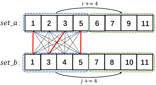
Figure 6: Merge-based Intersection with SIMD Instructions

We describe the main steps of the merge-based set intersection with SIMD instructions (Line 5) as follows [28, 35].

• Load vectors. Both two vectors of four $32$-bit integers are loaded into $128$-bit registers by SIMD load instructions such as $\_mm\_lddqu\_si128()$.

• Fully compare vectors. Make an all-pairs comparison between two vectors. First, compare four $32$-bit integers in both two vectors by SIMD compare instructions ($\_mm\_cmpeq\_epi32()$). Then shuffle one vector ($\_mm\_shuffle\_epi32()$) and repeat the comparison. Finally, store the intersection result ($\_mm\_storeu\_si128()$).

• Forward comparison. Compare the last elements of the two vectors. Advance both pointers to the next block when they are equal. Otherwise, the pointer of the smaller one is moved forward.

The intrinsic $\_mm\_lddqu\_si128()$ loads consecutive $128$-bit data from memory to a $128$-bit SIMD register; $\_mm\_cmpeq\_epi32(a,b)$ compares four $32$-bit integers in registers $a$ and $b$ for equality; $\_mm\_shuffle\_epi32(a,m)$ shuffles the four $32$-bit integers in the register $a$ with the mask $m$; $\_mm\_storeu\_si128()$ writes the $128$-bit data from the register to the result array.

Example 5.

In Fig.6, two vectors $V_{a}=set\_a[i:i+3]$ and $V_{b}=set\_b[j:j+3]$ are loaded into two $128$-bit registers with $\_mm\_lddqu\_si128()$. We compare the vectors with $\_mm\_cmpeq\_epi32()$ and get two common values $1$ and $5$. Then $V_{b}$ is shuffled as $[3,4,5,1]$, $[4,5,1,3]$ and $[5,1,3,4]$ with $\_mm\_shuffle\_epi32()$. We compare $V_{a}$ with each shuffled $V_{b}$ and get the common value $3$. Finally, the common values $[1,3,5,null]$ are written back to the result array with $\_mm\_storeu\_si128()$. We advance $i$ and $j$ to the next block (i.e., $i+=4,j+=4$) since $set\_a[i+3]=set\_b[j+3]$.

VII Optimization Strategies

VII-A Color Ordering

The main defect of other ordering heuristics is that the pruning effect is limited. They are based only on the size constraint that a $k$-clique must have at least k nodes. Color ordering [15] exploits the technique of greedy coloring [23], and prunes more unpromising search paths in the $k$-clique listing procedure. It is based on the following observation.

Lemma 1.

If $G_{k}$ contains a $k$-clique, then at least $k$ colors are needed to color $G_{k}$.

The greedy coloring colors the nodes following a fixed order, which is specified as the inverse degree ordering here. When coloring a vertex $v$, it always selects the minimum color value which has not been used by $v$’s neighbors. The greedy coloring colors each node in descending order of the degree, which tends to assign small color values to the high-degree nodes.

The color ordering first assigns a color value $c_{u}$ to each node $u$ with the greedy coloring. To construct the DAG $\mathop{G}\limits^{\rightarrow}$ by color ordering, the vertices are reordered based on the color values. Specifically, the orientation of $e=(u,v)$ is $u\rightarrow v$ if $c_{u}>c_{v}$. For the node $u\in\mathop{G}\limits^{\rightarrow}$ with $c_{u}<l$, the out-neighbors of $u$ have color values strictly smaller than $l-1$. Therefore, $u$ does not have $l-1$ out-neighbors with different colors, indicating that no $l$-clique rooted from $u$ exists.

Compared to the size constraint, the constraint of color values is stronger, which provides more pruning power. For example in Fig.7(b), since $v_{4}$ has $4$ out-neighbors, we can not prune $v_{4}$ based on the size constraint when finding a $5$-clique. However, the color value of $v_{4}$ is $4$, indicating that $v_{4}$ does not have $4$ out-neighbors with different colors. As a result, we can not find a $5$-clique rooted from $v_{4}$ and safely prune $v_{4}$.

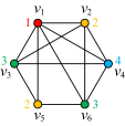
(a) Graph coloring

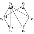
(b) DAG on color-ordering

Figure 7: The Example of Color Ordering

Example 6.

Assume the graph $G$ in Fig.7(a) is an induced subgraph, we generate the DAG $\mathop{G}\limits^{\rightarrow}$ based on the color ordering. Following the inverse degree ordering, the order for coloring the nodes is $(v_{1},v_{2},v_{3},v_{4},v_{6},v_{5})$. Firstly, $v_{1}$ is assigned with the smallest color value $1$, $v_{2}$ is colored with value $2$, then $v_{3}$ is colored with value $3$. Other nodes are colored similarly. As shown in Fig.7(b), the DAG $\mathop{G}\limits^{\rightarrow}$ is generated based on the color ordering.

VII-B Out-neighbor Reduction

In SDegree, we perform the set intersection between a candidate set $C$ and an out-neighbor set $N^{+}_{v}(\mathop{G}\limits^{\rightarrow})$ on each recursion. Initially, $C=N^{+}_{u}(\mathop{G}\limits^{\rightarrow})$ is the out neighbors of a certain vertex $u$. Some vertices of $N^{+}_{v}(\mathop{G}\limits^{\rightarrow})$ may not be in $N^{+}_{u}(\mathop{G}\limits^{\rightarrow})$, which causes unnecessary comparisons.

Motivated by the idea of induced subgraphs in [15, 12], we first construct the undirected subgraph $G_{u}$ induced by $N^{+}_{u}(\mathop{G}\limits^{\rightarrow})$ and list the ($k$-$1$)-cliques $C_{k-1}$ on $G_{u}$. All the $k$-cliques $C_{k}$ are listed as $\{u\}\cup C_{k-1}$. Therefore, we can efficiently prune the invalid nodes that will not be contained in $N^{+}_{u}(\mathop{G}\limits^{\rightarrow})$.

For the color-ordering based algorithms, the strategy of induced subgraphs can also be applied to reduce the worst-case time complexity [15]. We can first generate a DAG $\mathop{G}\limits^{\rightarrow}$ based on the degeneracy ordering. For each node $u$, we perform the ($k$-$1$)-clique listing on the undirected subgraph $G_{u}$ with color ordering.

VII-C More Efficient Set Intersection Strategies

We can efficiently reduce the set size for the intersection in two ways. On one hand, we perform the $k$-clique listing procedure on the undirected subgraph $G_{u}$ induced by $N^{+}_{u}(\mathop{G}\limits^{\rightarrow})$ for each node $u$. On the other, we exploit vertex ordering to reduce the maximum degree in $\mathop{G_{u}}\limits^{\rightarrow}$. After the neighbor set is greatly reduced, we can further accelerate the set intersections with the idea of bitmaps.

Firstly, we fix the size of nodes that a number can represent as $\mathcal{L}$. The vertex set $N^{+}_{u}(\mathop{G}\limits^{\rightarrow})$ is encoded as a vector $B_{u}$ with $\lceil d^{+}_{u}(\mathop{G}\limits^{\rightarrow})/\mathcal{L}\rceil$ numbers, and the out-neighbors of any node $v\in\mathop{G_{u}}\limits^{\rightarrow}$ are encoded as $B_{u}(v)$ with $\lceil d^{+}_{u}(\mathop{G_{u}}\limits^{\rightarrow})/\mathcal{L}\rceil$ numbers. The $i$-th bit of $B_{u}(v)$ is $1$, when the $i$-th out-neighbor of $u$ is also the out neighbor of $v$ in $\mathop{G_{u}}\limits^{\rightarrow}$. Meanwhile, a mask of $\mathcal{L}$-bits is calculated in advance, with which the neighbor sets can be recovered from a vector. Therefore, we can compress the neighbors of each node with a bitmap vector, instead of recording each specific neighbor in an adjacency list. Meanwhile, we only need to perform the bitwise AND operation based on the compressed neighbors, to obtain the intersection set that can further expand the current clique.

Example 7.

Let the graph in Fig.7(a) be an induced subgraph $G_{u}$ and Fig.7(b) be the DAG $\mathop{G_{u}}\limits^{\rightarrow}$ generated by color ordering. For $\mathcal{L}=3$, the compressed out-neighbor set of each vertex is shown in TABLE.III(a), and the corresponding mask is shown in TABLE.III(b). In this example, two numbers are needed to store each neighbor set in $\mathop{G_{u}}\limits^{\rightarrow}$. The intersection of $B_{u}(v_{3})$ and $B_{u}(v_{4})$ can be obtained with a bitwise AND operation $(\langle 3,2\rangle\&\langle 7,4\rangle=\langle 3,0\rangle)$, which can be recovered as $\{v_{1},v_{2}\}$ with the mask.

TABLE II: Bitmaps of Neighbor Sets

Bitmap	$v_{1}-v_{3}$	$v_{4}-v_{6}$
$B_{u}(u)$	$111(7)$	$111(7)$
$B_{u}(v_{1})$	$000(0)$	$000(0)$
$B_{u}(v_{2})$	$001(1)$	$000(0)$
$B_{u}(v_{3})$	$011(3)$	$010(2)$
$B_{u}(v_{4})$	$111(7)$	$100(4)$
$B_{u}(v_{5})$	$001(1)$	$000(0)$
$B_{u}(v_{6})$	$011(3)$	$010(2)$

(a) Encoding

Mask	Neighbors
$1(001)$	$\{v_{1}\}$
$2(010)$	$\{v_{2}\}$
$3(011)$	$\{v_{1},v_{2}\}$
$4(100)$	$\{v_{3}\}$
$5(101)$	$\{v_{1},v_{3}\}$
$6(110)$	$\{v_{2},v_{3}\}$
$7(111)$	$\{v_{1},v_{2},v_{3}\}$

(b) Decoding

VII-D BitCol

Based on the above optimizations, we propose our improved algorithm BitCol. First, a DAG $\mathop{G}\limits^{\rightarrow}$ is generated from $G(V,E)$, based on the degeneracy ordering. For each node $u$, BitCol constructs an undirected subgraph $G_{u}(V_{u},E_{u})$ induced by $N^{+}_{u}(\mathop{G}\limits^{\rightarrow})$. Specifically, $V_{u}=N^{+}_{u}(\mathop{G}\limits^{\rightarrow})$ and $E_{u}=\{(v_{i},v_{j})|(v_{i},v_{j})\in E,v_{i}\in V_{u},v_{j}\in V_{u}\}$. After that, a DAG $\mathop{G_{u}}\limits^{\rightarrow}$ is generated based on color ordering. Finally, BitCol iteratively processes on each induced subgraph $\mathop{G_{u}}\limits^{\rightarrow}$.

An appealing feature is that the size of vertices in each induced subgraph is restricted within the degeneracy $\beta$. Notice that the degeneracy is often very small in real-world graphs [30]. Therefore, we take the idea of bitmaps and propose a simple but effective strategy to accelerate the set intersections.

Input: A graph $G$ and a positive integer $k$

Output: All the $k$-cliques in $G$

1 Perform Pre-Core preprocessing on $G$

2 Perform Pre-List preprocessing on $G$

3 Generate a DAG $\mathop{G}\limits^{\rightarrow}$ based on degeneracy ordering

4 Fix $\mathcal{L}$ for bitmaps

5 for each node $u\in V(\mathop{G}\limits^{\rightarrow})$ do

6       if $d^{+}_{u}\geq k-1$ then

7             $R\leftarrow\{u\}$

8             $(\mathop{G_{u}}\limits^{\rightarrow},color)\leftarrow ColorOrdering(G_{u})$

9             $B_{u}\leftarrow BitEncode(\mathop{G_{u}}\limits^{\rightarrow},\mathcal{L})$

10             BitColList($k-1$, $color$, $R$, $B_{u}$, $B_{u}(u)$)

11            

12      

13Procedure BitColList($l$, $color$, $R$, $B$, $C_{B}$)

14 for each node $v\in BitDecode(C_{B})$ do

15       if $color(v)<l$ then

16             continue

17            

18       $C^{\prime}_{B}\leftarrow BitJoin(B(v),C_{B})$

19       if $l=2$ then

20             for each node $w\in BitDecode(C^{\prime}_{B})$ do

21                   output $k$-cliques $R\cup\{v,w\}$

22                  

23            

24       else

25             if $|BitDecode(C^{\prime}_{B})|)\geq l-1$ then

26                   BitColList($l-1$, $color$, $R\cup\{v\}$, $B$, $C^{\prime}_{B}$)

27                  

28            

29      

30Procedure BitJoin($B$, $C_{B}$)

31 for i = $1,2,\cdots,|B|$ do

       $C^{\prime}_{B}[i]\leftarrow B[i]\&C_{B}[i]$

        // Bitwise AND Operation

32      

return $C^{\prime}_{B}$

Algorithm 6 BitCol($G$, $k$)

As illustrated in Algorithm 6, BitCol first reduces the original graph by preprocessing (Lines 6-6). A DAG $\mathop{G}\limits^{\rightarrow}$ is generated based on degeneracy ordering. Then BitCol obtains the color values $color$ and the induced DAG $\mathop{G_{u}}\limits^{\rightarrow}$ by reordering the induced subgraph $G_{u}$ on color ordering (Line 6). After that, BitCol encodes the adjacency lists in $\mathop{G_{u}}\limits^{\rightarrow}$ with bitmaps, and invokes the procedure BitColList (Lines 6-6).

For the procedure BitColList, $R$ represents the current clique, $B$ is the bitmap, and $C_{B}$ is the encoded bitmap of the candidate set with which $R$ can be expanded into a $(|R|+1)$-clique. Before processing on each vertex $v$, BitColList decodes the bitmap of $C_{B}$ into the candidate set (Line 6). According to Lemma 1, BitColList prunes the search space for $color(v)<l$ (Lines 6-6). Since $color(v)<l$, $v$ does not have $l-1$ out neighbors with different colors, which means $v$ and its out neighbors can not form any $l$-clique.

BitColList accelerates the set intersections with the procedure BitJoin (Line 6), which performs bitwise AND operation on the candidate vector with bitmap $C_{B}$ and the encoded out-neighbor vector $B(v)$ (Lines 6-6). Note that the procedure BitJoin exploits the data level parallelism with the compiler auto-vectorization [24, 25], which can obtain further acceleration.

VII-E Data Parallelism with Auto-vectorization

Automatic vectorization is supported on Intel® 64 architectures [24, 25]. If vectorization is enabled (compiled using O2 or higher options), the compiler may use the additional registers to perform four bitwise operations in a single instruction. The obstacles to auto-vectorization are non-contiguous memory access and data dependencies, both of which are avoided by the Procedure BitJoin (Lines 6-6). However, the hash join accesses non-contiguous memory so that auto-vectorization can not be exploited.

For the original serial loop, each instruction can only handle single data. Instead, single instruction processes on a block of elements for the vectorized loop. For example, the loop in BitJoin can be vectorized as follows:

$$C_{B}^{\prime}[i:i+3]\leftarrow B[i:i+3]\&C_{B}[i:i+3],$$

where the loop bound is $\lfloor|B|/4\rfloor$ and single instruction can handle four results of the bitwise AND operation. The remaining ($|B|$ mod $4$) elements at the tail will be processed in a serial loop.

VIII Theoretical Analysis

In this section, we give a theoretical analysis of the correctness, time complexity, and space complexity of our algorithms. Let $m$ be the number of edges, $\Delta$ be the upper bound of the out-degree and $N$ be the number of threads. The state-of-the-art algorithms list all the $k$-cliques in $O(km(\frac{\Delta}{2})^{k-2})$ time, using $O(m+N\Delta^{2})$ memory.

The correctness is guaranteed by the unique listing order of the vertices which represent a $k$-clique.

Theorem 1 (Correctness).

Both SDegree and BitCol list every $k$-clique in $G$ without repetition.

Proof.

Obviously, Pre-Core and Pre-List will not affect the final results of $k$-clique listing. Let $\{v_{1},\dots,v_{k}\}$ be the nodes of a $k$-clique. There is the only ordering such that $\eta(v_{1})<\eta(v_{2})<\dots<\eta(v_{k})$. $\forall i\in[2,k]$, vertex $v_{i}$ will be detected after $v_{i-1}$ since $v_{i}\in N^{+}_{v_{i-1}}$. Therefore, the $k$-clique will only be listed in the order $(v_{1},v_{2},\dots,v_{k})$, without repetition. ∎

Theorem 2.

SDegree lists all the $k$-cliques with $O(m+kN\Delta)$ space and BitCol uses $O(m+N\Delta^{2}/\mathcal{L})$ space, where $\mathcal{L}$ is the size of nodes that each number can represent.

Proof.

The space overhead is mainly divided into two parts, the input original graph $G$ and each subgraph $G_{u}$ induced by $N^{+}_{u}$. Both SDegree and BitCol require $O(m)$ memory for storing the input graph $G$. Then we perform the analysis on the induced subgraph $G_{u}$.

SDegree only maintains the vertex set of $G_{u}$ in each recursion, which is the candidate set $C$ ($|C|\leq\Delta$). Therefore, SDegree requires additional $O(k\Delta)$ space for each thread ($k\leq\Delta$). For BitCol, each neighbor set of induced subgraph $G_{u}$ is compressed with a binary representation, where each number can represent $\mathcal{L}$ nodes. Therefore, BitCol requires additional $O(\Delta^{2}/\mathcal{L})$ space for each thread. ∎

To present a formal analysis of the time complexity, several necessary lemmas are given in the following. The $k$-clique listing problem can be solved in linear time for $\Delta<2$ or $k<3$. Therefore, we only consider $\Delta\geq 2$ and $k\geq 3$ in this paper.

Lemma 2.

Let $C$ be the candidate set for expanding the $k$-cliques. The time complexity of the procedure SDegreeList in Algorithm 5 can be upper bounded by $T(l,C)$ written as the following recurrence:

$$\left\{\begin{array}[]{ll}T(2,C)=2\sum\limits_{u\in C}(|C|+d^{+}_{u})\\ T(l,C)=\sum\limits_{u\in C}(|C|+d^{+}_{u})+\sum\limits_{u\in C}T(l-1,N^{+}_{u}\cap C)\end{array}\right.$$

Proof.

For each node $u\in C$, SDegreeList first calculates the intersection $C^{\prime}$ of $N^{+}_{u}$ and $C$, which runs in $O(\sum\limits_{u\in C}(|C|+d^{+}_{u}))$. If $l=2$, $k$-cliques of $R\cup\{u,v\}$ are reported for each node $v\in C^{\prime}$ ($O(\sum\limits_{u\in C}(|C|+d^{+}_{u}))$). Otherwise, SDegreeList is recursively executed with the new parameters $l-1$ and $C^{\prime}=N^{+}_{u}\cap C$. ∎

Lemma 3.

Let $C$ be the candidate set in Algorithm 5. For each node $u$, the following equation holds, where $\Delta$ is the upper bound of the out-degree in $\mathop{G}\limits^{\rightarrow}$.

$$\sum\limits_{u\in C}|N^{+}_{u}\cap C|\leq\frac{|C|(\Delta-1)}{2}$$

Proof.

Consider the subgraph $\mathop{G_{c}}\limits^{\rightarrow}(C,E_{c})$ induced by $C$ in $\mathop{G}\limits^{\rightarrow}$, where $E_{c}=\{\langle u,v\rangle|\langle u,v\rangle\in E(\mathop{G}\limits^{\rightarrow}),u\in C\wedge v\in C\}$. For each $u\in C$, $N^{+}_{u}(\mathop{G_{c}}\limits^{\rightarrow})=N^{+}_{u}(\mathop{G}\limits^{\rightarrow})\cap C$. Therefore, we have the following derivation.

$$\sum\limits_{u\in C}|N^{+}_{u}(\mathop{G}\limits^{\rightarrow})\cap C| =\sum\limits_{u\in C}|N^{+}_{u}(G_{c})|$$ (1)

$$\leq\frac{|C|(|C|-1)}{2}$$ (2)

$$\leq\frac{|C|(\Delta-1)}{2}$$ (3)

Equation (2) follows from the fact that $\sum\limits_{u\in C}|N^{+}_{u}(G_{c})|=|E_{c}|$, and $|E_{c}|$ is at most the number of edges in a $|C|$-clique. ∎

Lemma 4.

Let $\Delta$ be the upper bound of the out-degree in $\mathop{G}\limits^{\rightarrow}$ and $C$ be the candidate set in Algorithm 5, the following equation holds.

$$\begin{array}[]{ll}T(l,C)\leq 2\Delta(k+\frac{l}{2})(\frac{\Delta}{2})^{l-2}|C|\end{array}$$

Proof.

We prove by the induction on $l$, where $2\leq l\leq k-1$. For $l=2$ and $k\geq 3$, $T(2,C)=2\sum\limits_{u\in C}(|C|+d^{+}_{u})$. Obviously, we have $|C|\leq\Delta$ and $d^{+}_{u}\leq\Delta$ for each $u\in C$. Therefore, Lemma 4 holds for $l=2$. For $l>2$, we have the following derivation.

$$T(l,C) \leq\sum\limits_{u\in C}(|C|+d^{+}_{u})+\sum\limits_{u\in C}T(l-1,N^{+}_{u}\cap C)$$ (4)

$$\leq 2\Delta|C|+\sum\limits_{u\in C}2\Delta(k+\frac{l-1}{2})(\frac{\Delta}{2})^{l-3}|N^{+}_{u}\cap C|$$ (5)

$$=2\Delta|C|+2\Delta(k+\frac{l-1}{2})(\frac{\Delta}{2})^{l-3}\sum\limits_{u\in C}|N^{+}_{u}\cap C|$$ (6)

$$\leq 2\Delta|C|+2\Delta(k+\frac{l-1}{2})(\frac{\Delta}{2})^{l-2}|C|$$ (7)

$$\ \ \ -\Delta(k+\frac{l-1}{2})(\frac{\Delta}{2})^{l-3}|C|$$

$$\leq 2\Delta(k+\frac{l}{2})(\frac{\Delta}{2})^{l-2}|C|$$ (8)

Equation (4) follows from Lemma 2, Equation (5) follows from the inductive hypothesis, Equation (7) follows from Lemma 3, and Equation (8) follows from the fact that $2\Delta|C|\leq\Delta(k+\frac{l-1}{2})(\frac{\Delta}{2})^{l-3}|C|$ for $l>2$, $k\geq 3$, and $\Delta\geq 2$. ∎

Derived from Lemma 2 and Lemma 4, we can formally give the main theorems on the time complexity.

Theorem 3.

SDegree lists all the $k$-cliques in $O(km(\frac{\Delta}{2})^{k-2})$ time.

Proof.

According to Lemma 2, the time complexity of SDegree can be formulated as follows.

$$\begin{array}[]{ll}\mathcal{T}(k,G)=\sum\limits_{u\in V}T(k-1,N^{+}_{u})+O(m+n)\end{array}$$

First, Pre-Core and Pre-List both run in linear time. According to Lemma 4, we have the following derivation.

$$\mathcal{T}(k,G) =\sum\limits_{u\in V}T(k-1,N^{+}_{u})+O(m+n)$$

$$\leq\sum\limits_{u\in V}2\Delta(k+\frac{k-1}{2})(\frac{\Delta}{2})^{k-3}d^{+}_{u}+O(m+n)$$

$$\leq 6km(\frac{\Delta}{2})^{k-2}+O(m+n)$$

The last equation above follows from the fact that $\sum\limits_{u\in V}d^{+}_{u}=m$. ∎

Theorem 4.

BitCol lists all the $k$-cliques in $O(km(\frac{\Delta}{2})^{k-2})$ time.

Proof.

This theorem can be proved similarly as the Theorem 3. ∎

IX Experiments

TABLE III: Statistics of Datasets

Dataset	Name	$|V|$	$|E|$	$d_{avg}$	$\omega$	$N_{max}$
BerkStan	BS	685K	7M	19.41	201	4
Pokec	PK	1.6M	22.3M	27.32	29	6
DBLP	DB	317k	1M	6.62	114	1
CitPatents	CP	6M	16.5M	5.49	11	2
Linkedin	LK	6.7M	19.4M	5.76	11	33
Stanford	BB	282K	2M	14.14	61	10
WebUK05	UK05	129K	11.7M	181.19	500	2
ClueWeb09	CW	428M	446M	2.09	56	160
Wikipedia13	WP	27.1M	543M	40.01	428	4
AllWebUK02	UK02	18.5M	262M	28.27	944	1

In this section, we conduct extensive experiments to evaluate the efficiency of our algorithms SDegree and BitCol.

IX-A Experimental Setup

Settings. All experiments are carried on a Linux machine, equipped with 1TB disk, 128GB memory, and 4 Intel Xeon CPUs (4210R @2.40GHz, 10 cores). All algorithms are implemented in C/C++ and compiled with -O3 option. The source codes of DDegree and DDegCol  are publicly available in [15]. For all the algorithms, we set the time limit to 24 hours, and the reported running time is the total CPU time excluding only the I/O time of loading graph from disk.

Datasets. All datasets are downloaded from the public website NetworkRepository . The detailed data descriptions are demonstrated in TABLE III, where $d_{avg}$ denotes the average degree, $\omega$ denotes the maximum clique size, and $N_{max}$ denotes the number of maximum cliques.

If $\omega$ is large, the number of $k$-cliques is exponentially large with a relatively large $k$. For instance, BerkStan has $4$ $201$-cliques and each of them has around $1.8\times 10^{27}$ $20$-cliques, which can not be listed in a reasonable time for all the algorithms.

Algorithms. We compare two state-of-the-art algorithms DDegree and DDegCol for $k$-clique listing with our two proposed algorithms. We fix $\mathcal{L}=24$ for BitCol.

• DDegree is the state-of-the-art algorithm for degree ordering.

• DDegCol is the state-of-the-art algorithm for color ordering. For general $k$-clique listing algorithms, there does not exist a clear winner between DDegree and DDegCol [15], thus we compare both of them with our algorithms.

• SDegree is our proposed algorithm based on degree ordering.

• BitCol is our proposed algorithm based on color ordering.

To be more specific, we compare SDegree with DDegree for degree ordering, and compare BitCol with DDegCol for color ordering, respectively.

IX-B $k$-clique Listing Time in Serial

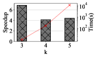
(a) AllWebUK02

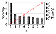
(b) Stanford

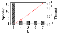
(c) BerkStan

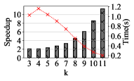
(d) CitPatents

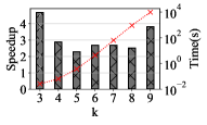
(e) DBLP

(f) Linkedin

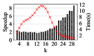
(g) Pokec

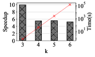
(h) WebUK05

Figure 8: Running Time on Degree Ordering. Red lines represent running time of SDegree; Histograms represent speedups of SDegree over DDegree.

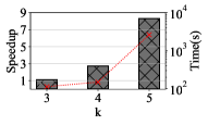
(a) AllWebUK02

(b) BerkStan

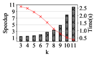
(c) CitPatents

(d) Stanford

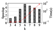
(e) DBLP

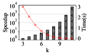
(f) Linkedin

(g) Pokec

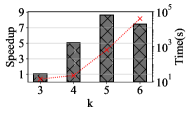
(h) WebUK05

Figure 9: Running Time on Color Ordering. Red lines represent running time of BitCol; Histograms represent speedups of BitCol over DDegCol.

In this experiment, we evaluate the $k$-clique listing time in serial with varying the size $k$. The experiments are conducted based on degree ordering and color ordering respectively, which are illustrated in Fig.8 and Fig.9. The red dotted line in Fig.8 represents the $k$-clique listing time of SDegree, and the histogram represents the speedup of SDegree over DDegree. Similarly, the red dotted line in Fig.9 represents the $k$-clique listing time of BitCol, and the histogram represents the speedup of BitCol over DDegCol. The results shown in Fig.8 and Fig.9 indicate that our algorithms outperform DDegree and DDegCol for fixed $k$, no matter based on degree ordering or color ordering.

From the perspective of the acceleration ratio w.r.t $k$, there are some interesting findings. In Fig.8, SDegree has a significant effect when dealing with triangle listing $(k=3)$. We explain that SDegree does not need to construct induced subgraphs, which requires additional time overhead. Correspondingly, BitCol only has a tiny speedup over DDegCol for triangle listing, since the listing process is dominated by constructing and reordering induced subgraphs when $k$ is small. The advantage of BitCol with bitmaps to accelerate the set intersections is gradually obvious as $k$ increases. This further demonstrates that the set intersection is an essential step in the process of $k$-clique listing.

Within the time limit, we compare the total time required for all data sets and for all $k$ in serial as a metric to calculate the speedups of our algorithms. In a word, SDegree outperforms DDegree by $3.75$x, and BitCol outperforms DDegCol by $5.67$x for the total time.

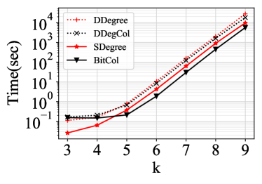
(a) DBLP

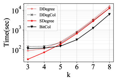
(b) ClueWeb09

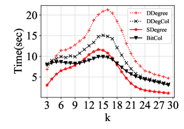
(c) Pokec

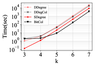
(d) BerkStan

Figure 10: Effect of $k$ after our preprocessing techniques

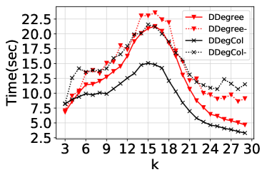
(a) Preprocessing (Pokec)

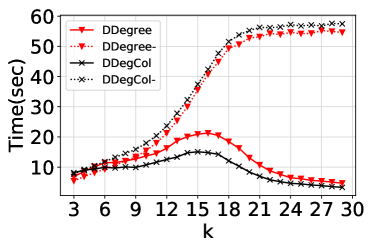
(b) Pruning (Pokec)

Figure 11: Comparison of preprocessing and pruning techniques on Pokec. DDegree- means DDegree without our preprocessing ($a$) or pruning techniques ($b$), so does DDegCol-.

Effect of $k$. DDegree and DDegCol can also exploit Pre-Core and Pre-List. Fig.10 illustrates SDegree, BitCol, DDegree, and DDegCol after our proposed preprocessing techniques. For DBLP, ClueWeb09, and BerkStan, it is in line with expectations that the listing time grows exponentially w.r.t $k$ since the number of $k$-cliques is exponential in the size $k$. However, it does not hold for Pokec where the time grows marginally or even decreases w.r.t $k$. An explanation would be that the maximum clique size $\omega$ is small, and most of the search space is pruned in the preprocessing stage. As shown in Fig.11(a), both DDegree and DDegCol run faster after our preprocessing techniques on Pokec. What’s more, the pruning effects of the color constraint and the size constraint become more and more obvious as $k$ increases, which is illustrated in Fig.11(b). Similar results can be obtained on Pokec for SDegree and BitCol.

When $k$ is small, degree-based algorithms run faster than color-based algorithms. For example, DDegree runs in $88$s and DDegCol runs in $144$s for ClueWeb09 and $k=3$ in Fig.10(b). Similar results can be observed for SDegree and BitCol. One explanation could be that the running time is dominated by greedy coloring.

Effect of Dataset. For a given $k$, the $k$-clique listing time varies in datasets with different graph topologies. The maximum clique size $\omega$ is closely related to the running time, determining the lower bound of time overhead. For example, the running time on DBLP is significantly higher than Pokec as $k$ increases for all the algorithms, even though the scale of DBLP is much smaller. This is because the maximum clique size of DBLP ($114$) is much larger than that of Pokec ($29$).

In Pokec, the running time for both the degree-ordering based and the color-ordering based algorithms first increases as $k$ increases to around $\omega/2$, and then drops as $k$ increases to $\omega$. The reason could be in two ways. First, our preprocessing and pruning techniques can prune more invalid nodes as $k$ increases in advance. Furthermore, the pruning performance becomes more effective for a larger $k$. For the sparse graph Linkedin in Fig.8 and Fig.9, most of the search space is pruned after the preprocessing, and we obtain up to three magnitudes of acceleration.

IX-C $k$-clique Listing Time in Parallel

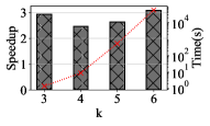
(a) AllWebUK02

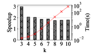
(b) Stanford

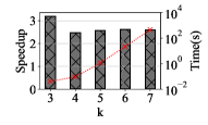
(c) BerkStan

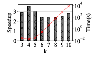
(d) DBLP

Figure 12: Running Time on Degree Ordering (NodeParallel). Red lines represent running time of $\textit{SDegree}_{32}$; Histograms represent speedups of $\textit{SDegree}_{32}$.

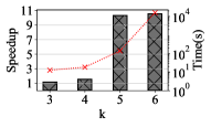
(a) AllWebUK02

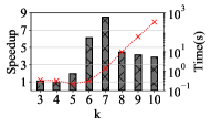
(b) Stanford

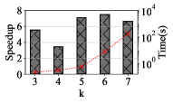
(c) BerkStan

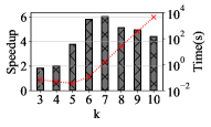
(d) DBLP

Figure 13: Running Time on Color Ordering (NodeParallel). Red lines represent running time of $\textit{BitCol}_{32}$; Histograms represent speedups of $\textit{BitCol}_{32}$.

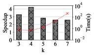
(a) BerkStan

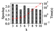
(b) Stanford

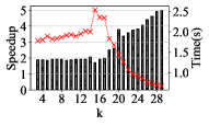
(c) Pokec

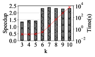
(d) DBLP

Figure 14: Running Time on Degree Ordering (EdgeParallel). Red lines represent running time of $\textit{SDegree}_{32}$; Histograms represent speedups of $\textit{SDegree}_{32}$.

(a) BerkStan

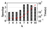
(b) Stanford

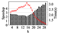
(c) Pokec

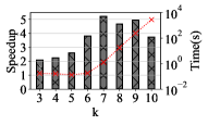
(d) DBLP

Figure 15: Running Time on Color Ordering (EdgeParallel). Red lines represent running time of $\textit{BitCol}_{32}$; Histograms represent speedups of $\textit{BitCol}_{32}$.

In this section, we conduct several experiments to evaluate the performance of SDegree and BitCol in the scenario of $32$ threads. We denote the parallel version of DDegree, SDegree, DDegCol, and BitCol as $\textit{DDegree}_{32}$, $\textit{SDegree}_{32}$, $\textit{DDegCol}_{32}$, and $\textit{BitCol}_{32}$.

Exp-I: NodeParallel with varying $k$. In this subsection, we evaluate the performance of our algorithms with the strategy of NodeParallel. More specifically, for each vertex $u\in G$, SDegree processes each candidate set $N^{+}_{u}$ in parallel, and each thread processes on each induced subgraph $G_{u}$ for BitCol. The experimental results are illustrated in Fig.12 and Fig.13.

Similarly, the running time grows exponentially w.r.t $k$ for most graphs. In parallel, all the algorithms further accelerate $k$-clique listing and are capable of listing larger cliques within the time limit. For example, we can list all the $6$-cliques in AllWebUK02 and $10$-cliques in DBLP, which is infeasible in serial. In general, $\textit{SDegree}_{32}$ outperforms $\textit{DDegree}_{32}$, and $\textit{BitCol}_{32}$ outperforms $\textit{DDegCol}_{32}$, respectively. In particular, $\textit{BitCol}_{32}$ achieves more speedup with multiple threads than BitCol, which implies that BitCol can make better use of parallelism. For example, $\textit{BitCol}_{32}$ achieves around $8$x speedup while BitCol achieves around $5$x speedup, for BerkStan and $k=6$.

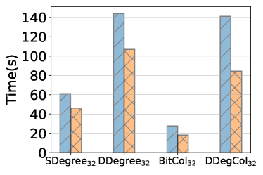
(a) DBLP ($k=8$)

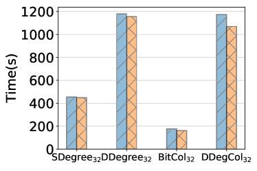
(b) BerkStan ($k=7$)

Figure 16: NodeParallel vs. EdgeParallel

Exp-II: NodeParallel vs. EdgeParallel. In this subsection, we evaluate the strategy of EdgeParallel [12]. The basic idea is that each thread handles the intersection of out-neighbors of one edge’s two endpoints. Compared to NodeParallel where the processing of each thread is based on the out-neighbors of one node, EdgeParallel processes “smaller” out-neighbor sets. Therefore, EdgeParallel can achieve a higher degree of parallelism.

Fig.16 shows the results on DBLP ($k=8$) and BerkStan ($k=7$). From Fig.16, the performance of NodeParallel is worse than that of EdgeParallel, indicating that EdgeParallel has a higher degree of parallelism.

As illustrated in Fig.14 and Fig.15, $\textit{SDegree}_{32}$ and $\textit{BitCol}_{32}$ still outperform $\textit{DDegree}_{32}$ and $\textit{DDegCol}_{32}$ with the strategy of EdgeParallel respectively, which also demonstrates the superiority of our algorithms.

IX-D Evaluation of Preprocessing Techniques

Exp-I: Preprocessing Time. In Table.IV, we evaluate the preprocessing time of DDegree, SDegree, DDegCol, and BitCol. For all datasets, we average the preprocessing time with varying $k$ within the time limit. The preprocessing time of DDegree and DDegCol is mainly dependent on the reordering of the original graph $G$ by degeneracy ordering, with a complete core decomposition. Both SDegree and BitCol apply the preprocessing techniques of Pre-Core and Pre-List. Since BitCol requires an additional reordering with degeneracy ordering, we merge Pre-Core with the complete core decomposition for BitCol.

In general, the preprocessing time of the four algorithms is almost the same, since all the techniques of preprocessing run in linear time. Meanwhile, we find that the preprocessing time of SDegree is slightly lower. This is because SDegree does not need to perform the complete core decomposition, where the Pre-Core can stop earlier when each vertex has a degree of no less than $k-1$. The preprocessing time of BitCol is a bit higher, since it exploits both the complete core decomposition and the Pre-List preprocessing. However, the speedup of BitCol can dominate the additional time consumption from preprocessing. For example, DDegCol lists all the $7$-cliques in ClueWeb09 within $3,188$ seconds, and BitCol is $1,943$ seconds faster, which is far more than the preprocessing time ($181$ seconds).

Exp-II: Efficiency of Preprocessing. As demonstrated in Fig.17, we evaluate the efficiency of our proposed preprocessing algorithms Pre-Core and Pre-List on Linkedin and Pokec. We compare the running time of the complete SDegree and BitCol algorithms with the no-preprocessing versions. It is shown that our preprocessing algorithms achieve around $1.5$x speedup for SDegree and BitCol in Pokec. Furthermore, we can achieve up to an order of magnitude acceleration for Linkedin. Our preprocessing algorithms improve the performance of SDegree and BitCol by removing invalid nodes that will not be contained in any $k$-clique.

TABLE IV: Average Preprocessing time of all algorithms

Dataset	SDegree	BitCol	DDegCol	DDegree
BerkStan	0.218s	0.283s	0.269s	0.267s
Pokec	1.347s	1.911s	1.801s	1.796s
DBLP	0.070s	0.101s	0.088s	0.090s
CitPatents	2.608s	3.556s	3.152s	3.154s
Linkedin	3.482s	4.698s	4.676s	4.659s
WebUK05	0.104s	0.152s	0.143s	0.146s
ClueWeb09	138.713s	181.113s	159.308s	161.204s
Wikipedia13	50.056s	67.318s	65.447s	64.361s
AllWebUK02	8.742s	14.063s	13.363s	13.401s
Stanford	0.130s	0.165s	0.157s	0.149s

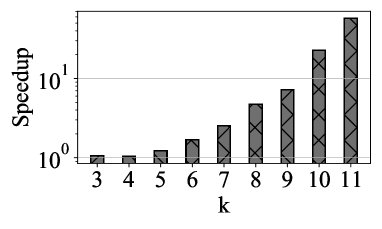
(a) Linkedin (SDegree)

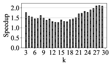
(b) Pokec (SDegree)

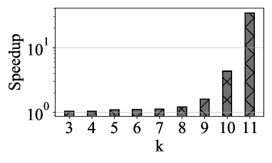
(c) Linkedin (BitCol)

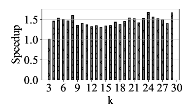
(d) Pokec (BitCol)

Figure 17: The efficiency of preprocessing (No preprocessing = $1.0$)

IX-E Evaluation of Memory Consumption

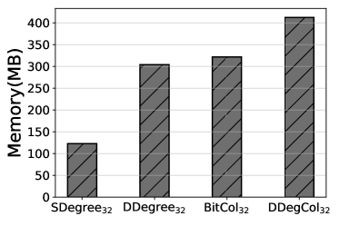
(a) Pokec ($k=18$)

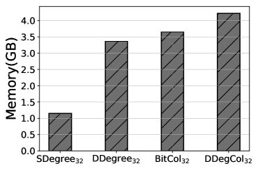
(b) AllWebUK02 ($k=4$)

Figure 18: Memory Consumption with 32 threads (NodeParallel)

We evaluate the memory consumption on Pokec ($k=18$) and AllWebUK02 ($k=4$) with NodeParallel and $32$ threads, which is shown in Fig.18. We can see that the memory overhead of $\textit{SDegree}_{32}$ is minimal. As we analyzed in Section VIII, $\textit{SDegree}_{32}$ does not require extra space to construct induced subgraphs. Moreover, the memory overhead of $\textit{BitCol}_{32}$ is smaller than that of $\textit{DDegCol}_{32}$ as expected, due to the capability of bitmap vectors to compress the out-neighbor sets. However, the memory overhead of $\textit{BitCol}_{32}$ is a bit larger than that of $\textit{DDegree}_{32}$ in Fig.18 since the color-based algorithms need to maintain additional information, such as color values.

X Conclusion

In this paper, we proposed two algorithms SDegree and BitCol to efficiently solve the $k$-clique listing problem, based on degree ordering and color ordering, respectively. We mainly focused on accelerating the set intersection part, thereby accelerating the entire process of $k$-clique listing. Both SDegree and BitCol exploit the data level parallelism, which is non-trivial for the state-of-the-art algorithms.

First, two preprocessing techniques Pre-Core and Pre-List are developed to efficiently prune the invalid nodes that will not be contained in a $k$-clique. SDegree is a simple but effective framework based on merge join while BitCol improves SDegree with bitmaps and color ordering. Our algorithms have comparable time complexity and a slightly better space complexity, compared with the state-of-the-art algorithms. We concluded from the experimental results that our algorithms outperform the state-of-the-art algorithms by $3.75$x for degree ordering and by $5.67x$ for color ordering on average.

Since a $k$-clique can be obtained by extending a vertex adjacent to all $k-1$ nodes in a $(k-1)$-clique, the existing algorithms are all based on the recursive framework to expand from a node to a $k$-clique. The state-of-the-art algorithms propose to exploit the ordering heuristics to prune invalid search space, while in this paper, we mainly focus on accelerating set intersections, which is a frequent operation in the recursive framework.

One inherent limitation for all the existing algorithms is that, when the size of the maximum clique ($\omega$) is large and $k$ is close to $\omega/2$, the problem of $k$-clique listing is often deemed infeasible. The existing algorithms take a significant amount of time to enumerate the $k$-cliques contained in the maximum cliques. Further studies can be conducted that whether we can enumerate the $k$-cliques within and outside the maximum (or near maximum) cliques separately.

References

- [1] Y. Dourisboure, F. Geraci, and M. Pellegrini, “Extraction and classification of dense implicit communities in the web graph,” ACM Trans. Web, vol. 3, no. 2, pp. 7:1–7:36, 2009.
- [2] C. E. Tsourakakis, “The k-clique densest subgraph problem,” in Proceedings of the 24th International Conference on World Wide Web, WWW 2015, Florence, Italy, May 18-22, 2015 (A. Gangemi, S. Leonardi, and A. Panconesi, eds.), pp. 1122–1132, ACM, 2015.
- [3] A. E. Sariyüce, C. Seshadhri, A. Pinar, and Ü. V. Çatalyürek, “Nucleus decompositions for identifying hierarchy of dense subgraphs,” ACM Trans. Web, vol. 11, no. 3, pp. 16:1–16:27, 2017.
- [4] C. Ma, Y. Fang, R. Cheng, L. V. S. Lakshmanan, W. Zhang, and X. Lin, “Efficient algorithms for densest subgraph discovery on large directed graphs,” in Proceedings of the 2020 International Conference on Management of Data, SIGMOD Conference 2020, online conference [Portland, OR, USA], June 14-19, 2020 (D. Maier, R. Pottinger, A. Doan, W. Tan, A. Alawini, and H. Q. Ngo, eds.), pp. 1051–1066, ACM, 2020.
- [5] B. Sun, M. Danisch, T. H. Chan, and M. Sozio, “Kclist++: A simple algorithm for finding k-clique densest subgraphs in large graphs,” Proc. VLDB Endow., vol. 13, no. 10, pp. 1628–1640, 2020.
- [6] A. Angel, N. Koudas, N. Sarkas, D. Srivastava, M. Svendsen, and S. Tirthapura, “Dense subgraph maintenance under streaming edge weight updates for real-time story identification,” VLDB J., vol. 23, no. 2, pp. 175–199, 2014.
- [7] X. Du, R. Jin, L. Ding, V. E. Lee, and J. H. T. Jr., “Migration motif: a spatial - temporal pattern mining approach for financial markets,” in Proceedings of the 15th ACM SIGKDD International Conference on Knowledge Discovery and Data Mining, Paris, France, June 28 - July 1, 2009 (J. F. E. IV, F. Fogelman-Soulié, P. A. Flach, and M. J. Zaki, eds.), pp. 1135–1144, ACM, 2009.
- [8] E. Fratkin, B. T. Naughton, D. L. Brutlag, and S. Batzoglou, “Motifcut: regulatory motifs finding with maximum density subgraphs,” in Proceedings 14th International Conference on Intelligent Systems for Molecular Biology 2006, Fortaleza, Brazil, August 6-10, 2006, pp. 156–157, 2006.
- [9] R. A. Hanneman and M. Riddle, “Introduction to social network methods,” 2005.
- [10] M. O. Jackson, Social and economic networks. Princeton university press, 2010.
- [11] L. Falzon, “Determining groups from the clique structure in large social networks,” Social networks, vol. 22, no. 2, pp. 159–172, 2000.
- [12] M. Danisch, O. Balalau, and M. Sozio, “Listing k-cliques in sparse real-world graphs,” in Proceedings of the 2018 World Wide Web Conference on World Wide Web, WWW 2018, Lyon, France, April 23-27, 2018 (P. Champin, F. Gandon, M. Lalmas, and P. G. Ipeirotis, eds.), pp. 589–598, ACM, 2018.
- [13] M. Latapy, “Main-memory triangle computations for very large (sparse (power-law)) graphs,” Theor. Comput. Sci., vol. 407, no. 1-3, pp. 458–473, 2008.
- [14] M. Yu, L. Qin, Y. Zhang, W. Zhang, and X. Lin, “AOT: pushing the efficiency boundary of main-memory triangle listing,” in Database Systems for Advanced Applications - 25th International Conference, DASFAA 2020, Jeju, South Korea, September 24-27, 2020, Proceedings, Part II (Y. Nah, B. Cui, S. Lee, J. X. Yu, Y. Moon, and S. E. Whang, eds.), vol. 12113 of Lecture Notes in Computer Science, pp. 516–533, Springer, 2020.
- [15] R. Li, S. Gao, L. Qin, G. Wang, W. Yang, and J. X. Yu, “Ordering heuristics for k-clique listing,” Proc. VLDB Endow., vol. 13, no. 11, pp. 2536–2548, 2020.
- [16] E. Gregori, L. Lenzini, and S. Mainardi, “Parallel $(k)$-clique community detection on large-scale networks,” IEEE Trans. Parallel Distributed Syst., vol. 24, no. 8, pp. 1651–1660, 2013.
- [17] G. Palla, I. Derényi, I. Farkas, and T. Vicsek, “Uncovering the overlapping community structure of complex networks in nature and society,” nature, vol. 435, no. 7043, pp. 814–818, 2005.
- [18] P. Hui and J. Crowcroft, “Human mobility models and opportunistic communications system design,” Philosophical Transactions of the Royal Society A: Mathematical, Physical and Engineering Sciences, vol. 366, no. 1872, pp. 2005–2016, 2008.
- [19] H. Saito, M. Toyoda, M. Kitsuregawa, and K. Aihara, “A large-scale study of link spam detection by graph algorithms (S),” in AIRWeb 2007, Third International Workshop on Adversarial Information Retrieval on the Web, co-located with the WWW conference, Banff, Canada, May 2007, vol. 215 of ACM International Conference Proceeding Series, 2007.
- [20] S. Jayanthi and S. Sasikala, “Clique-attacks detection in web search engine for spamdexing using k-clique percolation technique,” International Journal of Machine Learning and Computing, vol. 2, no. 5, p. 648, 2012.
- [21] B. Adamcsek, G. Palla, I. J. Farkas, I. Derényi, and T. Vicsek, “Cfinder: locating cliques and overlapping modules in biological networks,” Bioinform., vol. 22, no. 8, pp. 1021–1023, 2006.
- [22] N. Chiba and T. Nishizeki, “Arboricity and subgraph listing algorithms,” SIAM J. Comput., vol. 14, no. 1, pp. 210–223, 1985.
- [23] R. M. R. Lewis, A Guide to Graph Colouring - Algorithms and Applications. Springer, 2016.
- [24] C. Mendis, C. Yang, Y. Pu, S. P. Amarasinghe, and M. Carbin, “Compiler auto-vectorization with imitation learning,” in Advances in Neural Information Processing Systems 32: Annual Conference on Neural Information Processing Systems 2019, NeurIPS 2019, December 8-14, 2019, Vancouver, BC, Canada (H. M. Wallach, H. Larochelle, A. Beygelzimer, F. d’Alché-Buc, E. B. Fox, and R. Garnett, eds.), pp. 14598–14609, 2019.
- [25] D. Naishlos, “Autovectorization in gcc,” in Proceedings of the 2004 GCC Developers Summit, pp. 105–118, 2004.
- [26] H. Inoue, M. Ohara, and K. Taura, “Faster set intersection with SIMD instructions by reducing branch mispredictions,” Proc. VLDB Endow., vol. 8, no. 3, pp. 293–304, 2014.
- [27] D. Lemire, O. Kaser, N. Kurz, L. Deri, C. O’Hara, F. Saint-Jacques, and G. S. Y. Kai, “Roaring bitmaps: Implementation of an optimized software library,” Softw. Pract. Exp., vol. 48, no. 4, pp. 867–895, 2018.
- [28] S. Han, L. Zou, and J. X. Yu, “Speeding up set intersections in graph algorithms using SIMD instructions,” in Proceedings of the 2018 International Conference on Management of Data, SIGMOD Conference 2018, Houston, TX, USA, June 10-15, 2018 (G. Das, C. M. Jermaine, and P. A. Bernstein, eds.), pp. 1587–1602, ACM, 2018.
- [29] C. Bron and J. Kerbosch, “Finding all cliques of an undirected graph (algorithm 457),” Commun. ACM, vol. 16, no. 9, pp. 575–576, 1973.
- [30] D. Eppstein, M. Löffler, and D. Strash, “Listing all maximal cliques in large sparse real-world graphs,” ACM J. Exp. Algorithmics, vol. 18, 2013.
- [31] V. Batagelj and M. Zaversnik, “An o(m) algorithm for cores decomposition of networks,” CoRR, vol. cs.DS/0310049, 2003.
- [32] W. Zheng, Y. Yang, and C. Piao, “Accelerating set intersections over graphs by reducing-merging,” in KDD ’21: The 27th ACM SIGKDD Conference on Knowledge Discovery and Data Mining, Virtual Event, Singapore, August 14-18, 2021 (F. Zhu, B. C. Ooi, and C. Miao, eds.), pp. 2349–2359, ACM, 2021.
- [33] E. D. Demaine, A. López-Ortiz, and J. I. Munro, “Adaptive set intersections, unions, and differences,” in Proceedings of the Eleventh Annual ACM-SIAM Symposium on Discrete Algorithms, January 9-11, 2000, San Francisco, CA, USA (D. B. Shmoys, ed.), pp. 743–752, ACM/SIAM, 2000.
- [34] B. Ding and A. C. König, “Fast set intersection in memory,” Proc. VLDB Endow., vol. 4, no. 4, pp. 255–266, 2011.
- [35] B. Schlegel, T. Willhalm, and W. Lehner, “Fast sorted-set intersection using SIMD instructions,” in International Workshop on Accelerating Data Management Systems Using Modern Processor and Storage Architectures - ADMS 2011, Seattle, WA, USA, September 2, 2011 (R. Bordawekar and C. A. Lang, eds.), pp. 1–8, 2011.
- [36] C. S. A. Nash-Williams, “Decomposition of Finite Graphs Into Forests,” Journal of the London Mathematical Society, vol. s1-39, pp. 12–12, 01 1964.
- [37] M. C. Lin, F. J. Soulignac, and J. L. Szwarcfiter, “Arboricity, h-index, and dynamic algorithms,” Theoretical Computer Science, vol. 426, pp. 75–90, 2012.
- [38] D. Eppstein and E. S. Spiro, “The h-index of a graph and its application to dynamic subgraph statistics,” Journal of Graph Algorithms and Applications, vol. 16, no. 2, p. 543–567, 2012.