Emergent Universe from Energy-Momentum Squared Gravity

Abstract

In order to bypass the big bang singularity, we develop an emergent universe scenario within a covariant extension of General Relativity known as “Energy-Momentum Squared Gravity”. The extra terms of the model emerge in the high energy regime. Considering dynamics in a Friedmann-Lemaître-Robertson-Walker background, critical points, representing stable Einstein static states of the phase space, result as solutions. It then turns out that as the equation of state parameter $\omega$ gradually declines from a constant value as $t\rightarrow-\infty$, eventually some of the static past eternal solutions find the chance to naturally enter into thermal history through a graceful exit mechanism. In this way, the successful realization of the emergent universe allows an expanding thermal history without the big bang singularity for the spatially flat universe free of cosmological constant.

I Introduction

Although inflationary paradigm seems to be sufficiently supported by data so that one can take it as the default approach to describe the early universe, the initial singularity issue (the so-called Friedmann-Lemaître-Robertson-Walker (FLRW) big bang) is far from being clear and definitely solved in the framework of this paradigm. On the basis of some theorems Book , such singularities are generic and unavoidable, meaning that the classical spacetime has a threshold point beyond which the standard general relativity (GR) is not applicable Borde:1996pt ; Borde:2001nh . The singularities are commonly diagnosed by divergences of the scalar invariants of curvature or torsion tensors or the collapse of geodesics at some given points. Therefore, it seems that the initial singularity issue will potentially shed light on the answer to the question of whether our universe has a beginning or eternally existed. The lack of a solution for this fundamental issue in the context of inflationary cosmology motivated many authors to construct some pre-inflationary scenarios such as: emergent universe (EU) Ellis:2002we ; Ellis:2003qz , cyclic/ekpyriotic scenarios Khoury:2001wf ; Steinhardt:2001st ; Khoury:2003rt ; Barrow:2004ad which are commonly non-singular or past eternal. Motivations by the widespread belief that including a quantum gravity (QG) effects at very short scales leads to the natural disappearance of singularities has led to some other singularity free cosmological models Bojowald:2001xe ; Hossain:2009ru ; Battisti:2009zzb ; Alesci:2016xqa . Those models have been merely derived from semi-classical corrections to QG, see Ali:2014hma ; Vakili:2015wbw ; Khodadi:2016bcx , or considering non-local corrections Bahamonde:2017sdo ; Capozziello:2020xem as well.

The so-called EU scenario is one of the popular candidates that has been highly considered by several authors. This scenario, which is equivalent to “a creation in absence of beginning of time”, includes striking traits: no initial singularity (no beginning of time i.e infinite past), no horizon problem and no QG era. More exactly, Ellis et al Ellis:2002we ; Ellis:2003qz proposed a scenario to overcome the initial singularity within the framework of GR. In this framework a closed FLRW cosmology with a positive spatial curvature is preceded by an initially static state known as the Einstein Static Universe (ESU) in the eternal past (instead of a big bang singularity). Finally this closed FLRW is superseded by the inflationary era. According to this scenario, the closed universe has existed eternally, but eventually, at some point, it begins inflating Mukherjee:2006ds . As a result, there are two required conditions for the scenario to provide a successful description for fixing the initial singularity: a self-consistent exit from the ESU i.e. stable as well as a graceful exit from the ESU to the inflation. Note that the former and the latter are respectively necessary and sufficient conditions for the singularity circumvention so that the failure in satisfying any of the two conditions will cease the EU scenario. Failure to meet the former condition caused this scenario to face a challenge in the first place. The original EU scenario failed to solve the big bang singularity issue successfully since Barrow et al Barrow:2003ni discovered that the ESU in GR is not stable, meaning that the universe in such an initial static state is not able to survive for a long time against the existence of dominating perturbations. However, the extreme physical conditions expected in the early universe (such as those arising from quantization of gravity, or corrections to GR) may turn the stability situation of initial state in favor of EU scenario. In other words, due to the failure of the EU scenario in the context of GR, modified theories of gravity may have the potential to improve the situation. This idea has led to several studies on the natural extensions of the original EU setup into modified gravitational theories with the aim to derive some promising outputs in comparison with GR, Boehmer:2003iv -Sharif:2021 .

Recently, a modification of the matter Lagrangian (instead of gravitational Lagrangian) in a nonlinear way using a term proportional to $T_{\mu\nu}T^{\mu\nu}$ has been proposed as a new covariant generalization of GR Roshan:2016mbt ; Board:2017ign . This theory is known as “energy-momentum squared gravity” (EMSG) and induces quadratic contributions to gravity from matter side (without the appearance of novel forms of fluid stresses such as the scalar field and so on Akarsu:2018zxl ) so that it affects the cosmological dynamics considerably at high energy phases. In other words, the self-coupling of matter, instead of geometry, is assumed having interesting cosmological consequences, in particular, at early epochs. It is worth noticing that the so-called EMSG actually is a special case of theories with the general form of the Lagrangian as $f(R,T_{\mu\nu}T^{\mu\nu})$ which were first investigated in Arik:2013sti . Naturally, the expected deviations from GR in early universe can lead to non-trivial consequences for some key issues in modern cosmology such as: initial singularity, inflation and big bang nucleosynthesis. Actually due to the lack of a final theory of QG, one of the motivations behind considering modified gravities, such as EMSG, is trying to remove the big bang singularity. A previous work Roshan:2016mbt has shown that this theory is singularity free due to the bounce at early epochs. In other words, EMSG, by predicting a minimum length and a finite maximum energy density as common features of most QG approaches, cancels out the singularity issue of standard GR scenario of early universe. It is remarkable that it is the incentive to work with the EMSG model and also its generalized versions as it is not restricted to discarding the initial singularity, but, depending on the underlying EMSG model, it may result in some interesting modifications to the whole cosmic history, too. Other motivation for using EMSG come from trying to improve the usual paradigm in $\Lambda$CDM-based cosmology. Indeed, despite the $\Lambda$CDM is successful in fitting a wide range of the observational data, it not able to give a self-consistent description of the cosmic acceleration Capozziello:2011et . Tensions in measurements of the universe acceleration between early time and late time, as the so-called “Hubble tension”, may be a robust confirmation in the direction of modifying the $\Lambda$CDM picture as recently reported in DiValentino:2021izs . In other words, one may imagine the EMSG and its generalized models as phenomenological extensions of the $\Lambda$CDM, such that, despite the existence of a cosmological constant, the nonlinear matter Lagrangian, embedded in these models, leads to additional terms in Einstein’s equations, which finally can be constrained via cosmological observations. The cosmological applications of this novel modified theory of gravity along with its generalized types has attracted much attention in recent years (see some recent studies as Liu:2016qfx -Shahidi:2021lqf ). In Akarsu:2018zxl ; Ranjit:2020syg , the viability of EMSG has been studied via contrasting the relevant free parameter in light of observations. In Akarsu:2018zxl , authors used the existing observational constraints on the masses and radii of neutron stars and derived some constraints on the EMSG free parameter. In Ranjit:2020syg , by adopting recent observational data such as $i)$ cosmic chronometer and SNe Type-Ia Riess (292) $H(z)-z$ data-sets, $ii)$ baryon acoustic oscillation (BAO) peak parameter and $iii)$ cosmic microwave background (CMB) peak parameter, bounds on the model parameter $\alpha$ have been derived. It is worth mentioning that, for low redshift data, some constraints on the relevant model parameter of energy-momentum-powered gravity models have been achieved Faria:2019ejh . Although that constraints obtained on EMSG free parameter are tight, still this theory is at the play.

The above descriptions motivated us to look for another cosmological implication of EMSG model i.e. the full realization of the EU scenario. More exactly, we seek for the possibility whether EMSG model allows the EU scenario to be a viable solution of the early universe singularity. It is worth noticing that the study of the EU within the context of EMSG is well-motivated, because it changes the GR-based picture at early times, exactly when the EU scenario comes into play.

This manuscript is structured as follows. In Sec. II, we give a general review of the action as well as dynamical field equations in the framework of EMSG model. In Sec. III ,we extract ESU solutions related to the underlying gravity model and then investigate their stability using first order dynamical system analysis. In Sec. IV, we look for a realistic EU scenario via providing a graceful exit mechanism for the stable ESU solutions derived in Sec. III. Finally, we end the paper with a discussion summarized in Sec. V. Across this manuscript, for the signature of the spacetime metric, we will set the $(-,+,+,+)$ convention.

II Energy-Momentum Squared Gravity and Background Field equations

In EMSG model, the action can be written as Roshan:2016mbt ; Board:2017ign

$$S_{EMSG}=\frac{1}{2\kappa}\int\sqrt{-g}(R-2\Lambda+\alpha(T_{\mu\nu}T^{\mu\nu}))\ d^{4}x+\int L_{m}\sqrt{-g}\ d^{4}x,~{}~{}~{}\kappa\equiv 8\pi G$$ (1)

in which the Einstein-Hilbert action with a cosmological constant $\Lambda$ is extended via adding a self contracting term of energy-momentum tensor (EMT), $T_{\mu\nu}T^{\mu\nu}$. Here, $R$, $L_{m}$ and $\alpha$, respectively refer to the Ricci scalar, the matter Lagrangian density and a real constant which addresses the gravitational coupling strength of the underlying modification. The mass dimension of the EMSG parameter $\alpha$ is $[M]^{-6}$ and potentially can be any non-zero real value. So it is expected that, in early universe with high energy density, the EMSG is different from the standard GR so that, by going to lower energies, this deviation has to disappear. The action (1) can be re-express as follows

$$S_{EMSG}=\int\sqrt{-g}\big{(}\frac{R-2\Lambda}{2\kappa}+L_{m,eff}\big{)}\ d^{4}x,~{}~{}~{}L_{m,eff}=L_{m}+\frac{\alpha}{2\kappa}T_{\mu\nu}T^{\mu\nu}$$ (2)

Varying the above action with respect to the inverse metric, we acquire the following modified Einstein’s field equations

$$R_{\mu\nu}-\frac{1}{2}Rg_{\mu\nu}+\Lambda g_{\mu\nu}=\kappa T^{\text{eff}}_{\mu\nu}~{},$$ (3)

where we have defined

$$T^{\text{eff}}_{\mu\nu} =-\frac{2}{\sqrt{-g}}\frac{\delta(\sqrt{-g}L_{m,eff})}{\delta g^{\mu\nu}}$$

$$=T_{\mu\nu}+\frac{\alpha}{\kappa}\left(\frac{1}{2}T_{\alpha\beta}T^{\alpha\beta}g_{\mu\nu}+2L_{m}(T_{\mu\nu}-\frac{1}{2}g_{\mu\nu}T)+TT_{\mu\nu}-2T_{\mu}^{\alpha}T_{\nu\alpha}+4T^{\alpha\beta}\frac{\partial^{2}L_{m}}{\partial g^{\mu\nu}\partial g^{\alpha\beta}}\right)~{}~{}.$$

which clearly indicate that further degrees of freedom related to EMSG can be formally dealt under the standard of perfect fluids. See for example Capozziello:2018ddp . The above equations allow us to show that $\nabla^{\mu}T^{\text{eff}}_{\mu\nu}=0$ not $\nabla^{\mu}T_{\mu\nu}=0$ . It is assumed here that $L_{m}$ is free of derivatives of the metric components. By considering the perfect fluid form for the EMT, we have

$$T_{\mu\nu}=(\rho+p)U_{\mu}U_{\nu}+pg_{\mu\nu},~{}~{}~{}~{}~{}T_{\mu\nu}T^{\mu\nu}=\rho^{2}+3p^{2}$$ (5)

where $\rho$, $p$ and $U_{\mu}$ respectively denote the energy density, the pressure and the co-moving four-velocity satisfying the conditions, $U_{\mu}U^{\mu}=-1$, $\nabla_{\nu}U^{\mu}U_{\mu}=0$. Now by taking the Lagrangian $L_{m}=p$, the last term in the right hand side of Eq.(II) cancels so that after inserting Eq.(5) into it, the modified Einstein’s field equations finally read as

$$\begin{split}R_{\mu\nu}-\frac{1}{2}Rg_{\mu\nu}+\Lambda g_{\mu\nu}=\kappa((\rho&+p)U_{\mu}U_{\nu}+pg_{\mu\nu})+\alpha\left(\frac{1}{2}(\rho^{2}+3p^{2})g_{\mu\nu}+(\rho+p)(\rho+3p)U_{\mu}U_{\nu}\right).\end{split}$$ (6)

The right-hand side of the above equation indicates that we no longer deal with a standard perfect fluid but with an effective fluid. More precisely, the whole budget of EMT does not come from standard matter fields only but there are other contributions coming from the non-Einsteinian part of the gravitational interaction Carloni:2004kp ; Carloni:2007eu ; SantosdaCosta:2018ovq . The cosmological applications of such effective fluids, arising from generalized theories of gravity, have been considered in recent years, see e.g. Capozziello:2018ddp ; Capozziello:2019wfi ; Capozziello:2019qlt . The paradigm is that contributions coming from geometric degrees of freedom or further fields are brought to the r.h.s. of field equations and then the r.h.s. is globally considered as a source satisfying the Bianchi Identity. We want to investigate the implications of these field equations in cosmology. Therefore, we consider the FLRW cosmological models. Using the FLRW metric

$$ds^{2}=-dt^{2}+a^{2}(t)\left(\frac{dr^{2}}{1-kr^{2}}+r^{2}\left(d\theta^{2}+\sin^{2}\theta d\phi^{2}\right)\right),$$ (7)

characterized by the expansion scale factor $a(t)$ and the constant curvature parameter $k=-1,0,1$ (corresponding to spatially open, flat and closed universes respectively), we obtain the following modified dynamical equations

$$\frac{\dot{a}^{2}}{a^{2}}=-\frac{k}{a^{2}}+\frac{\Lambda}{3}+\kappa\frac{\rho}{3}+\frac{\alpha}{6}\left(\rho^{2}+3p^{2}+8\rho p\right),$$ (8)

and

$$\frac{\ddot{a}}{a}=-\kappa\frac{\rho+3p}{6}+\frac{\Lambda}{3}-\frac{\alpha}{3}\left(\rho^{2}+3p^{2}+2\rho p\right),$$ (9)

for an isotropic and homogeneous universe where dot means derivative with respect to the cosmic time. Assuming that in a spacetime with the FLRW background metric, the matter field obeys a barotropic equation of state (EoS), $p/\rho=w=Const$, then we can extend the dynamical equations expressed in the following final forms

$$\frac{\dot{a}^{2}}{a^{2}}=-\frac{k}{a^{2}}+\frac{\Lambda}{3}+\kappa\frac{\rho}{3}+\frac{\alpha A_{1}(w)}{3}\rho^{2},$$ (10)

and

$$\frac{\ddot{a}}{a}=-\kappa\frac{1+3w}{6}\rho+\frac{\Lambda}{3}-\frac{\alpha A_{2}(w)}{3}\rho^{2},$$ (11)

with constants $A_{1,2}(w)$ designated by

$$A_{1}(w)\equiv\frac{3}{2}w^{2}+4w+\frac{1}{2},\quad A_{2}(w)\equiv 3w^{2}+2w+1~{}.$$ (12)

Merging the above dynamical equations, we obtain

$$\dot{H}=-\frac{1+w}{2}\rho-\frac{\alpha}{3}(A_{1}+A_{2})\rho^{2}+\frac{k}{a^{2}},$$ (13)

where $H=\frac{\dot{a}}{a}$ and $\dot{H}=\frac{\ddot{a}}{a}-H^{2}$. Differentiating the Friedman equation (10), we see that the GR-based conservation equation also is modified as

$$\dot{\rho}+3\frac{\dot{a}}{a}(1+w)\rho\left(\frac{\kappa+\alpha\rho(1+3w)}{\kappa+2\alpha\rho A_{1}(w)}\right)=0.$$ (14)

The above modified conservation equation is the cosmological counterpart of $\nabla^{\mu}T^{\text{eff}}_{\mu\nu}=0$. It means that we do not have to demand conservation of the ordinary $T_{\mu\nu}$, but the whole right-hand side of Einstein equation (3), that is conservation of $T^{\text{eff}}_{\mu\nu}$. As a consistency check, one can see immediately that if $\alpha=0$, then dynamical equations (10), (11) as well as the modified conservation equation (14), reproduce exactly GR behaviors. Due to the fact that the source of the modification in the gravity model under consideration comes from the extension of EMT, it is quite natural that the modified terms in dynamical equations (10) and (11) appear as $\mathcal{O}(\rho^{2})$. Eqs. (10) and (11), together with (13), form a complete dynamical set to investigate the existence and stability status of static solutions, as a prerequisite for the realization of EU. Hereinafter, for simplicity we will set $\kappa=1$ in our calculations. However, the other values of $\kappa$ can be considered under the same standard.

III first order cosmological dynamics and stability analysis of Einstein static solutions

The system of Eqs. (10)-(13) admit static solutions characterized by $\dot{a}=\ddot{a}=\dot{\rho}=0$ (i.e. $a_{ES}=\rho_{ES}=$const) which address the ESU phase. Let us start with a flat FLRW metric. Considering the cosmological dynamical system with $k=0$ and applying this condition in Eqs. (10) and (11), we obtain the critical points (CPs) as follows

$$\mbox{CP:~{}A}~{}~{}~{}\rho_{ES}=\frac{-1\pm\sqrt{1-4\Lambda A_{1}\alpha}}{2A_{1}\alpha},$$ (15)

with any positive arbitrary value of $\frac{1}{a_{ES}^{2}}$. However, for the above CPs to be physically meaningful, we have to check the non-negative energy density condition $\rho_{ES}\geq 0$. Thus, the CPs $A_{\pm}$, are physically meaningful if

$$\begin{array}[]{ll}\Lambda=0,~{}~{}\alpha\neq 0,~{}~{}\bigg{(}w<-\frac{4+\sqrt{13}}{3},~{}~{}\mbox{or}~{}~{}-\frac{4+\sqrt{13}}{3}<w<\frac{-4+\sqrt{13}}{3}~{}~{}\mbox{or}~{}~{}w>\frac{-4+\sqrt{13}}{3}\bigg{)}\\ \Lambda<0,~{}~{}\alpha<0,~{}~{}\bigg{(}-\frac{4+\sqrt{13}}{3}<w<\frac{-4+\sqrt{13}}{3}~{}~{}\mbox{or}~{}~{}\frac{-4+\sqrt{13}}{3}<w\leq-\frac{4}{3}+\frac{\sqrt{26+\frac{3}{\alpha\Lambda}}}{3\sqrt{2}}\bigg{)}\\ \Lambda<0,~{}~{}0<\alpha<-\frac{3}{26\Lambda},~{}~{}\bigg{(}-\frac{4+\sqrt{13}}{3}<w<\frac{-4+\sqrt{13}}{3},~{}~{}\mbox{or}~{}~{}w>\frac{-4+\sqrt{13}}{3}\bigg{)}\\ \Lambda<0,~{}~{}\alpha>-\frac{3}{26\Lambda},~{}~{}\bigg{(}-\frac{4+\sqrt{13}}{3}<w\leq-\frac{4}{3}-\frac{\sqrt{26+\frac{3}{\alpha\Lambda}}}{3\sqrt{2}},~{}~{}\mbox{or}~{}~{}-\frac{4}{3}+\frac{\sqrt{26+\frac{3}{\alpha\Lambda}}}{3\sqrt{2}}\leq w<\frac{-4+\sqrt{13}}{3},~{}~{}\mbox{or}~{}~{}w>\frac{-4+\sqrt{13}}{3}\bigg{)}\\ \end{array}$$ (20)

and

$$\begin{array}[]{ll}\Lambda\geq 0,~{}~{}\alpha<0,~{}~{}w>\frac{-4+\sqrt{13}}{3}\\ \Lambda\geq 0,~{}~{}\alpha>0,~{}~{}-\frac{4+\sqrt{13}}{3}<w<\frac{-4+\sqrt{13}}{3}\\ \Lambda<0,~{}~{}0<\alpha<-\frac{3}{26\Lambda},~{}~{}-\frac{4+\sqrt{13}}{3}<w<\frac{-4+\sqrt{13}}{3},\\ \Lambda<0,~{}~{}\alpha>-\frac{3}{26\Lambda},~{}~{}\bigg{(}-\frac{4+\sqrt{13}}{3}<w\leq-\frac{4}{3}-\frac{\sqrt{26+\frac{3}{\alpha\Lambda}}}{3\sqrt{2}},~{}~{}\mbox{or}~{}~{}-\frac{4}{3}+\frac{\sqrt{26+\frac{3}{\alpha\Lambda}}}{3\sqrt{2}}\leq w<\frac{-4+\sqrt{13}}{3},~{}~{}\mbox{or}~{}~{}w>\frac{-4+\sqrt{13}}{3}\bigg{)}\\ \end{array}$$ (25)

respectively. So in case of satisfying any of conditions released in Eqs. (20) and (25), the physical meaning of the CPs $A_{\pm}$ can be guaranteed, respectively.

The dynamical systems with $k=\pm 1$ can be obtained by applying the condition related to ESU in Eqs. (10) and (11). We obtain the following CPs

$$\begin{array}[]{ll}\mbox{CP:~{}C}~{}~{}~{}\frac{1}{a_{ES}^{2}}=\frac{(1+3w)A_{1}\big{(}-1\pm\sqrt{1-\frac{16\Lambda A_{2}\alpha}{(1+3w)^{2}}}\big{)}^{2}}{48\alpha A_{2}^{2}}+\frac{(1+3w)\big{(}-1\pm\sqrt{1-\frac{16\Lambda A_{2}\alpha}{(1+3w)^{2}}}\big{)}}{12\alpha A_{2}}+\frac{\Lambda}{3},\\ \mbox{CP:~{}D}~{}~{}~{}\frac{1}{a_{ES}^{2}}=-\frac{(1+3w)A_{1}\big{(}-1\pm\sqrt{1-\frac{16\Lambda A_{2}\alpha}{(1+3w)^{2}}}\big{)}^{2}}{48\alpha A_{2}^{2}}-\frac{(1+3w)\big{(}-1\pm\sqrt{1-\frac{16\Lambda\alpha A_{2}}{(1+3w)^{2}}}\big{)}}{12\alpha A_{2}}-\frac{\Lambda}{3},\end{array}$$ (28)

with the energy density

$$\rho_{ES}=\frac{(1+3w)\big{(}-1\pm\sqrt{1-\frac{16\Lambda A_{2}\alpha}{(1+3w)^{2}}}\big{)}}{4A_{2}\alpha}$$ (29)

for both CPs. Note that the CPs $C_{\pm}$ and $D_{\pm}$ come from the closed and open universes, respectively. Here because of the added conditions $\frac{1}{a_{ES}^{2}}>0$ and $\rho_{ES}\geq 0$, the extraction of the limits on parameters $(w,~{}\alpha,~{}\Lambda)$ to ensure the physical meaning of the aforementioned CPs is very complicated. However, we will do that for CPs $C_{\pm}$ and $D_{\pm}$, via the parameter space plots in terms of $w-\alpha$ with some positive, negative and zero fixed values of $\Lambda$. For similar analysis in extended gravity theories, see e.g. Carloni:2004kp ; Carloni:2007eu ; SantosdaCosta:2018ovq .

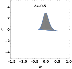
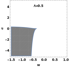
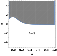
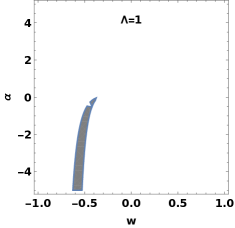
Figure 1: Regions of existence in the $(w,\alpha)$ parameter space for the stable CPs $C_{+}$ (up row) and $D_{+}$ (bottom row). $C_{+}$ and $D_{+}$ refer to the FLRW with $k=1$ and $k=-1$, respectively.

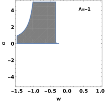
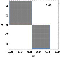
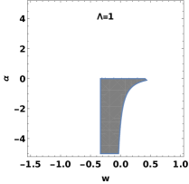
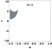
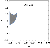
Figure 2: Regions of existence in the $(w,\alpha)$ parameter space for the stable CPs $C_{-}$ (up row) and $D_{-}$ (bottom row). $C_{-}$ and $D_{-}$ refer to the FLRW with $k=1$ and $k=-1$, respectively.

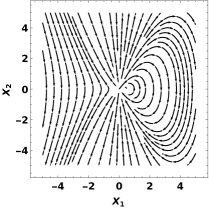
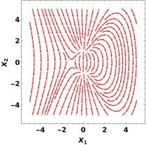
Figure 3: The phase diagram in $(a,\dot{a})$ or $(X_{1},X_{2})$ space for spatially flat, closed and open cosmology with the CPs $A_{-},~{}C_{+}$ and $D_{+}$, respectively from left to right panels. We use numerical values $(0,2,0)$, $(-0.8,-4,0.5)$ and $(0,5,-1)$ for the set parameters $(w,\alpha,\Lambda)$, respectively.

Now, in order to investigate the stability of these CPs, we follow the strategy that the second order dynamics of the cosmological model after introducing two variables $X_{1}=a,~{}~{}~{}X_{2}=\dot{a}$ can be reduced to the first order dynamics, as proposed for instance in Refs. Carneiro:2009et ; Wu:2009ah ; Zhang:2013ykz ; Huang:2015zma . Subsequently, we have a system of coupled equations as follows

$$\begin{array}[]{ll}\dot{X}_{1}=X_{2}=\mathcal{G}_{1}(X_{1},X_{2})~{},\\ \dot{X}_{2}=\frac{X_{2}^{2}}{X_{1}}-\bigg{(}\frac{1+w}{2}\rho+\frac{\alpha}{3}(A_{1}+A_{2})\rho^{2}\bigg{)}X_{1}+\frac{k}{X_{1}^{2}}=\mathcal{G}_{2}(X_{1},X_{2})~{}.\end{array}$$ (32)

The behavior of the coupled equations near the critical points can be studied by the Jacobian matrix of the coupled system. More precisely, the eigenvalues of the Jacobian matrix are related to the stability or instability of the system. Moreover, we extract the eigenvalues squared, $\lambda^{2}$, via the following Jacobian matrix

$$J\bigg{(}\mathcal{G}_{1}(X_{1},X_{2}),\mathcal{G}_{2}(X_{1},X_{2})\bigg{)}=\left(\begin{array}[]{cc}\frac{\partial\mathcal{G}_{1}}{\partial X_{1}}&\frac{\partial\mathcal{G}_{1}}{\partial X_{2}}\\ \frac{\partial\mathcal{G}_{2}}{\partial X_{1}}&\frac{\partial\mathcal{G}_{2}}{\partial X_{2}}\\ \end{array}\right)~{}~{}\Rightarrow~{}~{}~{}\lambda^{2}=\frac{\partial\mathcal{G}_{2}}{\partial X_{1}}|_{(a_{ES},\rho_{ES})}=$$ (35)

$$-\bigg{(}\frac{3}{2}\alpha w^{2}+2\alpha w+\frac{\alpha}{2}\bigg{)}\rho_{ES}^{2}-\frac{1+w}{2}\rho_{ES}-\frac{k}{a_{ES}^{2}}~{}.$$ (36)

When $\lambda^{2}<0$, we can consider the relevant physical CP as a stable ESU. Physically, $\lambda^{2}<0$ means that the relevant CP is a stable concentric center and if it undergoes some small perturbations, it does not collapse. In contrast, when $\lambda^{2}>0$, we expect to encounter an unstable saddle point .

Let us start our analysis with CPs $A_{\pm}$ which come from the flat FLRW case ($k=0$). By imposing the conditions $\lambda^{2}<0$ as well as $\rho_{ES}\geq 0$ simultaneously, we get the following constraints on the set $(w,\alpha,\Lambda)$

$$\begin{array}[]{ll}\Lambda<0,~{}~{}\alpha\leq\frac{3-\sqrt{13}}{4\Lambda}~{},~{}~{}-1<w<\sqrt{\frac{4}{54\alpha\Lambda+9}}-\frac{1}{3}\\ \Lambda<0,~{}~{}\frac{3-\sqrt{13}}{4\Lambda}<\alpha\leq\frac{1}{2\Lambda},~{}~{}\left(-1<w<\frac{\sqrt{13}-4}{3}~{}\mbox{or}~{}\frac{\sqrt{13}-4}{3}<w<\sqrt{\frac{4}{54\alpha\Lambda+9}}-\frac{1}{3}\right)\\ \Lambda<0~{},~{}~{}\frac{1}{2\Lambda}<\alpha<0,~{}~{}\left(-1<w<\frac{\sqrt{13}-4}{3},~{}\mbox{or}~{}\frac{\sqrt{13}-4}{3}<w\leq\sqrt{\frac{26\alpha\Lambda+3}{18\alpha\Lambda}}-\frac{4}{3}\right)\\ \Lambda<0,~{}~{}0<\alpha\leq-\frac{1}{8\Lambda},~{}~{}\left(-1<w<\frac{\sqrt{13}-4}{3}~{}\mbox{or}~{}w>\frac{\sqrt{13}-4}{3}\right)\\ \Lambda<0,~{}~{}-\frac{1}{8\Lambda}<\alpha\leq\frac{3}{4\Lambda}+\frac{\sqrt{13}}{4|\Lambda|},~{}~{}\left(-\sqrt{\frac{4}{54\alpha\Lambda+9}}-\frac{1}{3}<w\leq-\sqrt{\frac{26\alpha\Lambda+3}{18\alpha\Lambda}}-\frac{4}{3}~{}\mbox{or}~{}\right.\\ \left.\sqrt{\frac{26\alpha\Lambda+3}{18\alpha\Lambda}}-\frac{4}{3}\leq w<\frac{\sqrt{13}-4}{3}~{}\mbox{or}~{}w>\frac{\sqrt{13}-4}{3}\right)\\ \Lambda<0,~{}~{}\frac{3}{4\Lambda}+\frac{\sqrt{13}}{4|\Lambda|}<\alpha<-\frac{1}{6\Lambda},~{}~{}\left(-\sqrt{\frac{4}{54\alpha\Lambda+9}}-\frac{1}{3}<w<-\frac{4+\sqrt{13}}{3}~{}\mbox{or}~{}-\frac{4+\sqrt{13}}{3}<w\leq-\sqrt{\frac{26\alpha\Lambda+3}{18\alpha\Lambda}}-\frac{4}{3}~{}\mbox{or}~{}\right.\\ \left.\sqrt{\frac{26\alpha\Lambda+3}{18\alpha\Lambda}}-\frac{4}{3}\leq w<\frac{\sqrt{13}-4}{3}~{}\mbox{or}~{}w>\frac{\sqrt{13}-4}{3}\right)\\ \Lambda<0,~{}~{}\alpha\geq-\frac{1}{6\Lambda},~{}~{}\left(w<-\frac{4+\sqrt{13}}{3}~{}\mbox{or}~{}-\frac{4+\sqrt{13}}{3}<w\leq-\sqrt{\frac{26\alpha\Lambda+3}{18\alpha\Lambda}}-\frac{4}{3}~{}\mbox{or}~{}\sqrt{\frac{26\alpha\Lambda+3}{18\alpha\Lambda}}-\frac{4}{3}\leq w<\frac{\sqrt{13}-4}{3}~{}\mbox{or}\right.\\ \left.w>\frac{\sqrt{13}-4}{3}\right)\end{array}$$ (47)

and

$$\begin{array}[]{ll}\Lambda=0,~{}~{}\alpha<0,~{}~{}w>\frac{1}{3}\\ \Lambda=0,~{}~{}\alpha>0,~{}\left(-\frac{4+\sqrt{13}}{3}<w<-1~{}\mbox{or}~{}-1<w<\frac{\sqrt{13}-4}{3}\right)\\ \Lambda>0,~{}~{}-\frac{1}{6\Lambda}<\alpha<0,~{}~{}w>\sqrt{\frac{4}{54\alpha\Lambda+9}}-\frac{1}{3}\\ \Lambda>0,~{}~{}\alpha>0,~{}~{}\left(-\frac{4+\sqrt{13}}{3}<w<-1~{}\mbox{or}~{}-\sqrt{\frac{4}{54\alpha\Lambda+9}}-\frac{1}{3}<w<\frac{\sqrt{13}-4}{3}\right)\\ \Lambda<0,~{}~{}\frac{1}{2\Lambda}<\alpha<0,~{}~{}\sqrt{\frac{4}{54\alpha\Lambda+9}}-\frac{1}{3}<w\leq\sqrt{\frac{26\alpha\Lambda+3}{18\alpha\Lambda}}-\frac{4}{3}\\ \Lambda<0,~{}~{}0<\alpha\leq-\frac{1}{8\Lambda},~{}~{}\left(-\frac{4+\sqrt{13}}{3}<w<-\sqrt{\frac{4}{54\alpha\Lambda+9}}-\frac{1}{3}~{}\mbox{or}~{}-1<w<\frac{\sqrt{13}-4}{3}\right)\end{array}$$ (54)

respectively corresponding to the CPs $A_{+},~{}A_{-}$. As a result, CPs $A_{\pm}$ can address the physical stable ESUs in the context of EMSG model with a flat spacetime, if the above conditions are satisfied.

Let’s go to CPs $C_{\pm}$ and $D_{\pm}$ arising from the spatially non-flat cases. Here, by imposing the conditions $\rho_{ES}\geq 0$ and $\frac{1}{a_{ES}^{2}}>0$ along with the stability condition $\lambda^{2}<0$, it is not possible to list constraints such as (47) and (54). Instead we illustrate the parameter space plots in terms of $w-\alpha$ which address the allowed regions for existence of real and stable ESUs, see Figs. 1 and  2. As it is clear, the only CP which admits three values for the cosmological constant is $C_{-}$. The CPs $C_{+}$ and $D_{+}$ admit values $\Lambda<0$ and $\Lambda>0$ while for the CP $D_{-}$ just the value $\Lambda<0$ is allowed. As an additional check, in the Fig. 3 optionally for three CPs $A_{-},~{}C_{+}$ and $D_{+}$, we present the phase-space behavior for various set parameters $(w,\alpha,\Lambda)$.

An important issue has to be clarified at this point. The EMSG scenario modifies GR in the early phase of the universe. According to this statement, the CPs seem no longer applicable in classical evolution, because, in the EMSG phase, the universe undergoes a quantum regime. In this situation, the classical evolution and expansion seem forbidden. To address this concern, one has to note the following discussion. In Roshan:2016mbt , it is shown that, in the EMSG picture, by controlling the values of free parameter $\alpha$, the universe no longer enter a quantum era during its evolution. In other words, to guarantee that the CPs are free from quantum effects and allow the classical evolution, one has to impose additional conditions as $\rho_{ES}<\rho_{p}$ and $a_{ES}<\ell_{p}$ where $\rho_{p}$ and $\ell_{p}$ are the Planck energy density and the Planck length, respectively. More precisely, in our set up, the above mentioned constraints read as $\frac{1}{a_{ES}^{2}}<8\pi$ and $\rho_{ES}<64\pi$ since $c,~{}\hbar,~{}\kappa=1$ and $G=\frac{1}{8\pi}$. All numerical values taken into account for the EMSG parameter $\alpha$ throughout this paper satisfy both constraints, indicating that our analysis is safely classic and there is no need for any quantum considerations on the CPs. According to this result, the classical evolution is allowed.

III.1 Non-Singular oscillations around stable ESU(s)

To ensure that the previous results do show stable points, we perform analysis of small perturbations around the ESU phases. In what follows, we will show that if we impose some small perturbations around the above mentioned stable CPs (in particular spatially non-flat cases), the perturbations will undergo an infinite series of non-singular oscillations around the inception state. For this purpose, we linearly perturb Eqs. (10) and (11) around the ESUs. We define the perturbations in the scale factor and matter density as follows

$$a(t)\rightarrow a_{ES}(1+\delta a(t)),$$

$$\rho(t)\rightarrow\rho_{ES}(1+\delta\rho(t))~{},$$ (55)

and also we have the linear expansions

$$(1+\delta a(t))^{n}\simeq 1+n\delta a(t),$$

$$(1+\delta\rho(t))^{n}\simeq 1+n\delta\rho(t).$$ (56)

After discarding the cross differential and non-linear terms, Eq. (10) yields

$$\frac{\delta\rho}{\delta a}=-\frac{6k}{a_{ES}^{2}(\rho_{ES}+2\alpha A_{1})}~{}.$$ (57)

In the same way, using Eq. (III.1) to perturb Eq. (11) and replacing the above relation, we acquire

$$\delta\ddot{a}-\bigg{(}\frac{(1+3w)k\rho_{ES}+4\alpha kA_{2}\rho_{ES}^{2}}{a_{ES}^{2}(\rho_{ES}+2\alpha A_{1})}\bigg{)}\delta a=0~{}.$$ (58)

Now Eq. (58) allows us to consider the stability of the CPs extracted previously, via an alternative way i.e. a small perturbation around CPs. As a cross-check by turning off the coupling parameter $\alpha$ in Eq. (58), we recover what is expected in the context of standard GR Barrow:2003ni . In Figs. 4 and  5, we represent the evolution of the scale factor derived from Eq. (58) corresponding to CPs $C_{\pm}$ and $D_{\pm}$ with some optional parameters consistence with Figs. 1 and  2. We observe the universe displays small oscillations around the relevant ESUs.

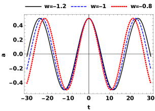
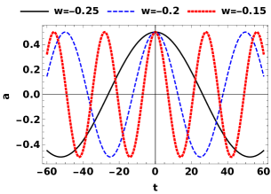
Figure 4: The evolutionary curves of scale factor corresponding to CPs $C_{-}$ (left panel) and $C_{+}$ (right panel) in terms of time with different values of $w$ and numerical values $\Lambda=0.5,~{}\alpha=-1$ and $\Lambda=0,~{}\alpha=-1$, respectively.

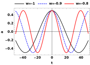
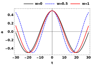
Figure 5: The evolutionary curves of scale factor corresponding to CPs $D_{-}$ (left panel) and $D_{+}$ (right panel) in terms of time with different values of $w$ and numerical values $\Lambda=-1,~{}\alpha=2$ and $\Lambda=-0.5,~{}\alpha=5$, respectively.

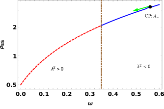
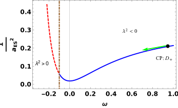
Figure 6: The general trend of transition of CPs $A_{-}$ corresponding to $\Lambda=0,~{}\alpha<0$ (left panel) and $D_{+}$ corresponding to $\Lambda<0,~{}\alpha>0$ (right panel) from stable region with $\lambda^{2}<0$ towards the unstable region with $\lambda^{2}>0$, as $\omega$ decreases. The vertical brown dashed-dotted line represents the critical value of $\omega$ where this transition occurs.

IV The realization of emergent cosmology scenario

In this section, we intend to find a graceful exit mechanism for the stable CPs in order to enter the standard thermal history of the universe by joining the CPs to the inflationary period. More precisely, by slowly reducing the universe equation of state parameter $w$, we look for a phase transition from a stable state to an unstable one for the aforementioned ESU solutions (CPs). In this way, we deal with a non-singular early universe in a stable state which finally will emerge in a standard expanding universe.

We start with CPs derived for the spatially flat case i.e. $A_{\pm}$. To extract a stable to unstable phase transition we need to know under what conditions the underlying CPs are both physical and unstable. Hence, for CPs $A_{\pm}$, we demand the conditions $\lambda^{2}>0$ as well as $\rho_{ES}\geq 0$. This will yield the following constraints on the set parameters $(w,\alpha,\Lambda)$

$$\begin{array}[]{ll}\Lambda<0,~{}~{}\alpha<\frac{3-\sqrt{13}}{4\Lambda}~{},~{}~{}\left(-\sqrt{\frac{26\alpha\Lambda+3}{18\alpha\Lambda}}-\frac{4}{3}\leq w<-\frac{4+\sqrt{13}}{3}~{}\mbox{or}~{}-\frac{4+\sqrt{13}}{3}<w<-1~{}\mbox{or}~{}\right.\\ \left.\sqrt{\frac{4}{54\alpha\Lambda+9}}-\frac{1}{3}<w<\frac{\sqrt{13}-4}{3}~{}\mbox{or}~{}\frac{\sqrt{13}-4}{3}<w\leq\sqrt{\frac{26\alpha\Lambda+3}{18\alpha\Lambda}}-\frac{4}{3}\right)\\ \Lambda<0,~{}~{}\alpha=\frac{3}{4\Lambda}-\frac{\sqrt{13}}{4|\Lambda|},~{}~{}\left(-\sqrt{\frac{26\alpha\Lambda+3}{18\alpha\Lambda}}-\frac{4}{3}\leq w<-\frac{4+\sqrt{13}}{3}~{}\mbox{or}~{}-\frac{4+\sqrt{13}}{3}<w<-1~{}\mbox{or}~{}~{}\right.\\ \left.\frac{\sqrt{13}-4}{3}<w\leq\sqrt{\frac{26\alpha\Lambda+3}{18\alpha\Lambda}}-\frac{4}{3}\right)\\ \Lambda<0~{},~{}~{}\frac{1}{2\Lambda}<\alpha<0,~{}~{}\left(-\sqrt{\frac{26\alpha\Lambda+3}{18\alpha\Lambda}}-\frac{4}{3}\leq w<\frac{1}{3},~{}\mbox{or}~{}-\frac{\sqrt{13}+4}{3}<w<-1\right)\\ \Lambda<0,~{}~{}0<\alpha\leq-\frac{3}{26\Lambda},~{}~{}\left(w<-\frac{\sqrt{13}+4}{3}~{}\mbox{or}~{}-\frac{\sqrt{13}+4}{3}<w<-1\right)\\ \Lambda<0,~{}~{}-\frac{3}{26\Lambda}<\alpha<-\frac{1}{8\Lambda}~{},~{}~{}\left(w<-\frac{4+\sqrt{13}}{3}~{}\mbox{or}~{}-\frac{4+\sqrt{13}}{3}<w\leq-\sqrt{\frac{26\alpha\Lambda+3}{18\alpha\Lambda}}-\frac{4}{3}~{}\mbox{or}~{}\sqrt{\frac{26\alpha\Lambda+3}{18\alpha\Lambda}}-\frac{4}{3}\leq w<-1\right)\\ \Lambda<0,~{}~{}\alpha=-\frac{1}{8\Lambda},~{}~{}\left(w<-\frac{4+\sqrt{13}}{3}~{}\mbox{or}~{}-\frac{4+\sqrt{13}}{3}<w<-\sqrt{\frac{26\alpha\Lambda+3}{18\alpha\Lambda}}-\frac{4}{3}\right)\\ \Lambda<0,~{}~{}-\frac{1}{8\Lambda}<\alpha<\frac{3}{4\Lambda}+\frac{\sqrt{13}}{4|\Lambda|},~{}~{}\left(w<-\frac{3}{4\Lambda}+\frac{\sqrt{13}}{4|\Lambda|}~{}\mbox{or}~{}-\frac{4+\sqrt{13}}{3}<w<-\sqrt{\frac{4}{54\alpha\Lambda+9}}-\frac{1}{3}\right)\\ \Lambda<0,~{}~{}\alpha=\frac{3}{4\Lambda}+\frac{\sqrt{13}}{4|\Lambda|},~{}~{}w<-\frac{4+\sqrt{13}}{3}\\ \Lambda<0,~{}~{}\frac{3}{4\Lambda}+\frac{\sqrt{13}}{4|\Lambda|}<\alpha<-\frac{1}{6\Lambda},~{}~{}w<-\sqrt{\frac{4}{54\alpha\Lambda+9}}-\frac{1}{3}\end{array}$$ (70)

and

$$\begin{array}[]{ll}\Lambda=0,~{}~{}\alpha<0,~{}~{}\left(w<-\frac{4+\sqrt{13}}{3}~{}\mbox{or}~{}\frac{\sqrt{13}-4}{3}<w<\frac{1}{3}\right)\\ \Lambda>0,~{}~{}\alpha\leq-\frac{1}{6\Lambda},~{}~{}\left(w<-\frac{4+\sqrt{13}}{3}~{}\mbox{or}~{}w>\frac{\sqrt{13}-4}{3}\right)\\ \Lambda>0,~{}~{}-\frac{1}{6\Lambda}<\alpha<0,~{}~{}\left(w<-\frac{4+\sqrt{13}}{3}~{}\mbox{or}~{}\frac{\sqrt{13}-4}{3}<w<\sqrt{\frac{4}{54\alpha\Lambda+9}}-\frac{1}{3}\right)\\ \Lambda>0,~{}~{}\alpha>0,~{}~{}-1<w<-\sqrt{\frac{4}{54\alpha\Lambda+9}}-\frac{1}{3}\\ \Lambda<0,~{}~{}\alpha<\frac{1}{2\Lambda},~{}~{}\left(-\sqrt{\frac{26\alpha\Lambda+3}{18\alpha\Lambda}}-\frac{4}{3}\leq w<-\frac{4+\sqrt{13}}{3}~{}\mbox{or}~{}\frac{\sqrt{13}-4}{3}<w\leq\sqrt{\frac{26\alpha\Lambda+3}{18\alpha\Lambda}}-\frac{4}{3}\right)\\ \Lambda<0,~{}~{}\alpha=\frac{1}{2\Lambda},~{}~{}\left(-\sqrt{\frac{26\alpha\Lambda+3}{18\alpha\Lambda}}-\frac{4}{3}\leq w<-\frac{4+\sqrt{13}}{3}~{}\mbox{or}~{}\frac{\sqrt{13}-4}{3}<w<\sqrt{\frac{26\alpha\Lambda+3}{18\alpha\Lambda}}-\frac{4}{3}\right)\\ \Lambda<0,~{}~{}\frac{1}{2\Lambda}<\alpha<0,~{}~{}\left(-\sqrt{\frac{26\alpha\Lambda+3}{18\alpha\Lambda}}-\frac{4}{3}\leq w<-\frac{4+\sqrt{13}}{3}~{}\mbox{or}~{}\frac{\sqrt{13}-4}{3}<w<\sqrt{\frac{4}{54\alpha\Lambda+9}}-\frac{1}{3}\right)\\ \Lambda<0,~{}~{}0<\alpha\leq-\frac{3}{26\Lambda},~{}~{}-\sqrt{\frac{4}{54\alpha\Lambda+9}}-\frac{1}{3}<w<-1\\ \Lambda<0,~{}~{}-\frac{3}{26\Lambda}<\alpha<-\frac{1}{8\Lambda},~{}~{}\left(-\sqrt{\frac{4}{54\alpha\Lambda+9}}-\frac{1}{3}<w\leq-\sqrt{\frac{26+3}{18\alpha\Lambda}}-\frac{4}{3}~{}\mbox{or}~{}\sqrt{\frac{26\alpha\Lambda+3}{18\alpha\Lambda}}-\frac{4}{3}\leq w<-1\right)\end{array}$$ (80)

respectively.

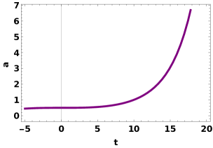
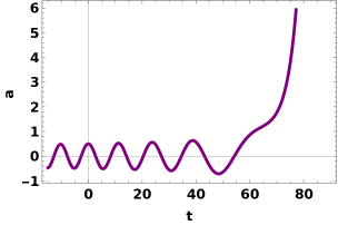
Figure 7: The graceful exit of ESU from a stable state to an inflationary epoch by supposing a gradually decreasing equation of state parameters $w(t)=0.33-0.001t$ and $w=-0.3-0.01t$ for the EMSG model with flat and spatially open geometries from left to right panels, respectively. We set numerical values ($\alpha=-1,~{}\Lambda\geq 0$) and ($\alpha=0.5,~{}\Lambda=-1$) with common initial conditions $a(0)=0.5$ and $\dot{a}(0)=0$ for left and right panels, respectively.

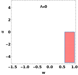
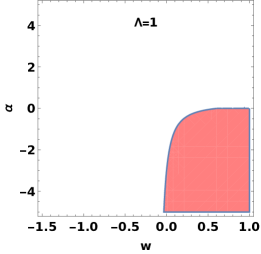
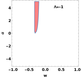
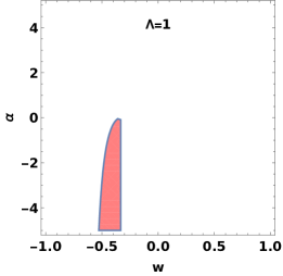
Figure 8: Regions of existence in the $(w,\alpha)$ parameter space for the unstable CPs $C_{-}$ (up row) and $D_{+}$ (bottom row).

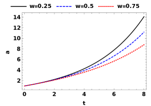
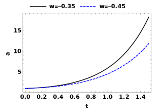
Figure 9: The increasing exponential behavior of the scale factor corresponding to the unstable CPs $C_{-}$ (left panel) and $D_{+}$ (right panel) with different values of $\omega$ and other numerical values related to Fig. 8.

Concerning the realization of the emergent universe scenario via the exit from the ESU, the CPs $A_{\pm}$ show some promising behavior.

In general, we expect this transition to be achieved in two ways, as the universe equation of state parameter slowly drops from a constant value in past ($t\rightarrow-\infty$). Either via changing the stability status of each of CPs separately from stable to unstable or exchanging a stable CP with its unstable counterpart so that finally we will deal with an unstable CP Wu:2009ah ; Zhang:2013ykz ; Huang:2015zma ; Khodadi:2015fav ; Khodadi:2016gyw . Note that in both ways, it is expected that the phase transition occurs for a critical value of $\omega$.

Concerning the former, one can find from terms in Eqs. (47) and  (70) that for the CP $A_{+}$ with negative cosmological constant and negative values for the modified parameter $\alpha$, there is the possibility of the transition discussed above. By a closer inspection after comparing the first cases in Eqs. (47) and (70), we note that by setting values $\Lambda=-1,~{}\alpha=-1$, for spatially flat geometry, we can achieve a stable ESU filled by a matter with the equation of state parameter $w$ around $-1$. However, the CP $A_{+}$ is no longer stable after gradually dropping $w$ below $-1$, meaning that it undergoes a stable-unstable phase transition. Comparing the third cases in Eqs. (47) and (70), we can also have a stable ESU, but this time filled by a matter with the equation of state parameter $w$ around $0$. After gradually decreasing $w$ below $0$, the CP $A_{+}$ exits from its stable status (for example, by setting values $\Lambda=-1,~{}\alpha=-1/4$). It turns out that this does not happen for positive values of $\alpha$.

Concerning CP $A_{-}$, we see from comparison of the first cases in Eqs. (54) and (80) that if $\Lambda=0,~{}\alpha<0$ then the phase transition does occur for a ESU filled by normal matter with the equation of state parameter $w$ around $1/3$. The third cases in Eqs. (54) and  (80) along with fifth item in Eq. (54) and the seventh in Eq. 80, signal the relevant phase transition for $\Lambda>0$ and $\Lambda<0$ but with $\alpha<0$, respectively. Given the admitted non-negative values for the cosmological constant by observation, the CPs relevant to $\Lambda\geq 0$ with $\alpha<0$ seem to be favored. Besides, the constraint obtained from the neutron stars on the coupling parameter $\alpha$ implies that the EMSG model with $\alpha<0$, also has the potential to adapt with observation Akarsu:2018zxl . Also, newly in the light of observational data analysis of cosmic chronometers and Supernovae Type Ia data, shown that the flat EMSG model with $\alpha<0$ result in a favor and consistency cosmology in the absence of cosmological constant Ranjit:2020syg . In Roshan:2016mbt , also by setting the opposite sign convention to action (1) i.e. $R-\alpha T_{\mu\nu}T^{\mu\nu}$, it is clearly discussed that in de Sitter universe with a flat geometry to have a well-behaved cosmology in late-time which is stable, it is required that $\alpha<0$. As a result of this discussion, the cases $\Lambda\geq 0,~{}\alpha<0$ are favored. In the left panel of Fig.  6, we schematically show the general trend of the transition of CP $A_{-}$, corresponding to $\Lambda=0,~{}\alpha<0$, from a stable region to an unstable one, as $\omega$ decreases and reaches a critical value.

Now we focus on the latter possibility for realization of phase transition. Comparing the third item in Eq. (47) with the seventh in Eq. (80), one finds that by setting values $\Lambda<0,~{}\frac{1}{2\Lambda}<\alpha<0$ for spatially flat geometry we can have a stable ESU addressed by CP $A_{+}$ filled by a matter with the equation of state parameter $w$ around $-1$. However, by gradually decreasing $w$ from $-1$ then the stable CP $A_{+}$ is exchanged with the unstable CP $A_{-}$. This describes a stable-unstable phase transition. The sixth and fifth (also sixth) items in Eqs. (54) and (70) respectively show that there is also the possibility of transition from stable CP $A_{-}$ to unstable CP $A_{+}$ for positive values of $\alpha$ but with $\Lambda<0$. If the an anti-de Sitter universe finds any support by evidence, this case with $\alpha>0$ can be favored. Left panel in Fig. 7 qualitatively displays the graceful exit from a stable state to inflation for the most popular possible case between mentioned above cases (i.e $\Lambda\geq 0$ and $\alpha<0$).

Considering the non-flat spatial geometries, let us start with closed universe ($k=+1$). By demanding instability conditions $\lambda^{2}>0$ , $\rho_{ES}\geq 0$ and $\frac{1}{a_{ES}^{2}}>0$ at the same time for the CPs $C_{\pm}$, we deal with allowed regions in $(w,\alpha)$ parameter space (Fig. 8). First of all, it is required that the scale factor no longer oscillates but grows exponentially to reach the inflationary phase. This can be done by setting the numerical values related to the allowed regions of Fig. 8 into the perturbed Eq. (58), as displayed in Fig. 9.

Interestingly, we find that the CP $C_{+}$ with non of the values of a cosmological constant admits these conditions. However, this is not the case for the CP $C_{-}$ with $\Lambda\geq 0$, as one can see in Fig. 8 (up row). By comparing these plots with its stable counterpart in Fig. 2 (up row), one recognizes that the stable-unstable phase transition is not possible as a result of the gradual decline of the equation of state parameter. However, by going to the spatially open geometry case, we realize that just for the CP $D_{+}$ the underlying phase transition will happen. More explicitly, the bottom row plots in Figs.  1 and 8, address a stable ESU full of normal matter filled with $w\geq 0$ for case of $\Lambda=-1$ and $\alpha>0$ which with the passage of time and decline of $w$, it is finally converted to an unstable state describing a phase transition. The right panel of Fig.  6, schematically shows the general trend of a transition from a stable region to an unstable one, as $w$ decreases. The right panel of Fig. 7 also qualitatively shows the graceful exit from a stable state to inflation for the CP $D_{+}$, as the time passes.

V Discussion and Conclusions

Aiming to circumvent the initial singularity issue in the FLRW cosmology, we investigate one of the scenarios under the spotlight in recent years named the Emergent Universe Scenario. Based on this scenario, our universe does not stem from an origin as a big bang singularity, but it comes from an Einstein static state in an infinite past and finally joins the inflationary period. The original framework for implementing this scenario was GR. Because GR does not admit a stable static universe, this led to the failure of this scenario in the first steps. Subsequent studies have shown that taking into account some mechanisms, such as effects of modified gravity, quantum gravity and extra dimensions, could improve original results in favor of the realization of Emergent Universe Scenario.

In this paper, we have implemented the Emergent Universe Scenario considering a modification of Einstein gravity known as Energy-Momentum Squared Gravity (EMSG) which is distinguished from its standard counterpart by the correcting term $T_{\mu\nu}T^{\mu\nu}$ in the action, that is considering a self-interaction of stress-energy tensor. By applying this theory into cosmology, some modified terms, addressed by the coupling parameter $\alpha$, appear in the Friedmann equations describing the dynamics of universe. These new terms can affect the original Emergent Universe Scenario.

As a first step, we started our analysis by extracting the static critical points known as Einstein Static Universe as a central concept in the study of the Emergent Universe Scenario. By employing a first order dynamical analysis within the phase space parameterized by $\alpha$, we found some stable static critical points for any three possible spatial geometries ($k=0,\pm 1$) in the absence and presence of cosmological constant $\Lambda>0~{}(<0)$.

In the next step, by finding a phase transition from a stable to an unstable state for these extracted static critical points, we investigated the graceful exist of the Einstein Static Universe superseded by an inflationary epoch. More precisely, the main idea is that for $t\rightarrow-\infty$, the value of $\omega$ is constant and the universe, in essence, has been eternally stuck in the stable Einstein static state until it finally comes out naturally from this state and evolves into an inflationary period, if $\omega$ drops slowly as time goes forward. It is worth noticing that when we say the Einstein Static Universe is stable or unstable, the statement is true only within a specified range of $w$. Besides, in the downward trend of $w$, at times when the cosmic $w$ approaches to critical values, some stable static solutions find the chance to exit from the allowed range of $w$ and, in this way, they enter into an unstable range of $w$, meaning that the standard universe evolution takes place. This can be seen schematically in Fig. 6 for the static solutions $A_{-}$ and $D_{+}$. As a result, this transition from stable to unstable Einstein Static Universe can be imagined natural in the sense that it occurs in two separated ranges of $w$, as the parameter decreases according to the time evolution.

Interestingly, we found that, in the context of EMSG, unlike the original idea in the standard general relativity, the realization of an emergent universe scenario does not impose a positive spatial curvature ($k=+1$). In the other words, our analysis have revealed that here the possibility of having an emergent universe for a closed universe, is ruled out. However, for both spatially flat $k=0$ and open $k=-1$ cases, under some constraints on the parameters ($\Lambda,\omega,\alpha$), there is the possibility of a perfect realization for the Emergent Universe Scenario. From three aspects, the most impressive output is related to the spatially flat case with $\Lambda=0$ and $\alpha<0$.

First, the spatially flat universe seems to be favored by cosmological data, also if the new Planck measurements could question this statement according to the discussion in DiValentino:2019qzk ; Vagnozzi:2020rcz . We leave its confirmation/rejection to the next data in the future.

Second, the Emergent Universe Scenario works in the absence of a cosmological constant. This fact could be relevant in view of solving the cosmological constant problem Weinberg:1988cp .

Third, it seems that the negative values of free model parameter $\alpha$ is supported by some observational constraints derived in Akarsu:2018zxl ; Ranjit:2020syg .

Our analysis, meanwhile, have shown that, in the spatially flat case with $\alpha>0$, there exists the possibility of a successful realization for the emergent universe if $\Lambda<0$, which despite its major role in AdS/CFT correspondence and a fundamental theory such as string, however, it is not supported by the cosmological observations. According to our analysis, by the Emergent Universe Scenario in the context of EMSG, it is possible to bypass the initial singularity considering some favorable conditions as well as in absence of quantum corrections. Results of our analysis become remarkable considering those reported in Barbar:2019rfn where it is shown that the initial bounce, expected from EMSG Roshan:2016mbt , is not viable as a regular bounce. This means that finding a bounce solution is not a sufficient condition to remove the singularity. On the other hand, we have shown that it is possible via a full realization of the Emergent Universe Scenario.

A further comment is worth at this point. The analysis of Emergent Universe Scenario can become richer, if one takes into account the presence of scalar fields in the EMSG Lagrangian density. This is due to the fact that EMSG not only changes the gravitational sector also modifies dynamics of all involved matter fields. So, by considering scalar fields in the Lagrangian density, due to the higher derivative terms $T_{\mu\nu}T^{\mu\nu}$ in (1), non-trivial effects come out in the Emergent Universe Scenario.

References

- (1) S. W. Hawking and G. F. R. Ellis, The large scale structure of Space-Time, Cambridge (1973).
- (2) A. Borde and A. Vilenkin, Int. J. Mod. Phys. D 5, 813 (1996) [gr-qc/9612036].
- (3) A. Borde, A. H. Guth and A. Vilenkin, Phys. Rev. Lett. 90, 151301 (2003) [gr-qc/0110012].
- (4) R. H. Brandenberger, AIP Conf. Proc. 1268, 3 (2010) [arXiv:1003.1745 [hep-th]].
- (5) R. H. Brandenberger, Lect. Notes Phys. 863, 333 (2013) [arXiv:1203.6698 [astro-ph.CO]].
- (6) R. Penrose, Annals N. Y. Acad. Sci. 571, 249 (1989).
- (7) G. F. R. Ellis and R. Maartens, Class. Quant. Grav. 21, 223 (2004) [gr-qc/0211082].
- (8) G. F. R. Ellis, J. Murugan and C. G. Tsagas, Class. Quant. Grav. 21, no. 1, 233 (2004) [gr-qc/0307112].
- (9) J. Khoury, B. A. Ovrut, P. J. Steinhardt and N. Turok, Phys. Rev. D 64, 123522 (2001) [hep-th/0103239].
- (10) P. J. Steinhardt and N. Turok, Phys. Rev. D 65, 126003 (2002) [hep-th/0111098].
- (11) J. Khoury, P. J. Steinhardt and N. Turok, Phys. Rev. Lett. 92, 031302 (2004) [hep-th/0307132].
- (12) J. D. Barrow, D. Kimberly and J. Magueijo, Class. Quant. Grav. 21, 4289 (2004) [astro-ph/0406369].
- (13) M. Bojowald, Phys. Rev. Lett. 86, 5227 (2001) [gr-qc/0102069].
- (14) G. M. Hossain, V. Husain and S. S. Seahra, Phys. Rev. D 81, 024005 (2010) [arXiv:0906.2798 [astro-ph.CO]].
- (15) M. V. Battisti, Phys. Rev. D 79, 083506 (2009).
- (16) E. Alesci, G. Botta, F. Cianfrani and S. Liberati, Phys. Rev. D 96, no. 4, 046008 (2017) [arXiv:1612.07116 [gr-qc]].
- (17) A. F. Ali and B. Majumder, Class. Quant. Grav. 31, no. 21, 215007 (2014) [arXiv:1402.5104 [gr-qc]].
- (18) B. Vakili and M. A. Gorji, Int. J. Mod. Phys. D 25, no. 02, 1650028 (2016) [arXiv:1511.03785 [gr-qc]].
- (19) M. Khodadi, K. Nozari and H. R. Sepangi, Gen. Rel. Grav. 48, no. 12, 166 (2016) [arXiv:1602.02921 [gr-qc]].
- (20) S. Capozziello, M. Capriolo and S. Nojiri, Phys. Lett. B 810, 135821 (2020) [arXiv:2009.12777 [gr-qc]].
- (21) S. Bahamonde, S. Capozziello and K. F. Dialektopoulos, Eur. Phys. J. C 77, no. 11, 722 (2017) [arXiv:1708.06310 [gr-qc]].
- (22) E. Di Valentino, A. Melchiorri and J. Silk, Nat. Astron. 4, no. 2, 196 (2019) [arXiv:1911.02087 [astro-ph.CO]].
- (23) S. Vagnozzi, E. Di Valentino, S. Gariazzo, A. Melchiorri, O. Mena and J. Silk, Phys. Dark Univ. 33, 100851 (2021) arXiv:2010.02230 [astro-ph.CO].
- (24) A. S. Eddington, Mon. Not. Roy. Astron. Soc. 90, 668 (1930).
- (25) G. Lemaître, Mon. Not. Roy. Astron. Soc. 91, 483 (1931).
- (26) S. Mukherjee, B. C. Paul, N. K. Dadhich, S. D. Maharaj and A. Beesham, Class. Quant. Grav. 23, 6927 (2006) [gr-qc/0605134].
- (27) J. D. Barrow, G. F. R. Ellis, R. Maartens and C. G. Tsagas, Class. Quant. Grav. 20, L155 (2003) [gr-qc/0302094].
- (28) C. G. Boehmer, Class. Quant. Grav. 21, 1119 (2004) [gr-qc/0310058].
- (29) D. J. Mulryne, R. Tavakol, J. E. Lidsey and G. F. R. Ellis, Phys. Rev. D 71, 123512 (2005) [astro-ph/0502589].
- (30) L. Parisi, M. Bruni, R. Maartens and K. Vandersloot, Class. Quant. Grav. 24, 6243 (2007) [arXiv:0706.4431 [gr-qc]].
- (31) C. G. Boehmer, L. Hollenstein and F. S. N. Lobo, Phys. Rev. D 76, 084005 (2007) [arXiv:0706.1663 [gr-qc]].
- (32) N. Goheer, R. Goswami and P. K. S. Dunsby, Class. Quant. Grav. 26, 105003 (2009) [arXiv:0809.5247 [gr-qc]].
- (33) R. Goswami, N. Goheer and P. K. S. Dunsby, Phys. Rev. D 78, 044011 (2008) [arXiv:0804.3528 [gr-qc]].
- (34) S. Carneiro and R. Tavakol, Phys. Rev. D 80, 043528 (2009) [arXiv:0907.4795 [astro-ph.CO]].
- (35) P. Wu and H. W. Yu, Phys. Rev. D 81, 103522 (2010) [arXiv:0909.2821 [gr-qc]].
- (36) C. G. Boehmer and F. S. N. Lobo, Eur. Phys. J. C 70, 1111 (2010) [arXiv:0909.3986 [gr-qc]].
- (37) L. Parisi, N. Radicella and G. Vilasi, Phys. Rev. D 86, 024035 (2012) [arXiv:1207.3922 [gr-qc]].
- (38) K. Zhang, P. Wu and H. Yu, Phys. Rev. D 85, 043521 (2012) [arXiv:1202.1397 [gr-qc]].
- (39) K. Zhang, P. Wu and H. Yu, JCAP 1401, 048 (2014) [arXiv:1311.4051 [gr-qc]].
- (40) K. Atazadeh, Y. Heydarzade and F. Darabi, Phys. Lett. B 732, 223 (2014) [arXiv:1401.7638 [gr-qc]].
- (41) S. Bag, V. Sahni, Y. Shtanov and S. Unnikrishnan, JCAP 1407, 034 (2014) [arXiv:1403.4243 [astro-ph.CO]].
- (42) M. Khodadi, Y. Heydarzade, K. Nozari and F. Darabi, Eur. Phys. J. C 75, no. 12, 590 (2015) [arXiv:1505.00342 [gr-qc]].
- (43) Q. Huang, P. Wu and H. Yu, Phys. Rev. D 91, no. 10, 103502 (2015) [arXiv:1504.05284 [gr-qc]].
- (44) Y. Heydarzade and F. Darabi, JCAP 1504, 028 (2015) [arXiv:1501.02624 [gr-qc]].
- (45) M. Khodadi, Y. Heydarzade, F. Darabi and E. N. Saridakis, Phys. Rev. D 93, no. 12, 124019 (2016) [arXiv:1512.08674 [gr-qc]].
- (46) M. Khodadi, K. Nozari and E. N. Saridakis, Class. Quant. Grav. 35, no. 1, 015010 (2018) [arXiv:1612.09254 [gr-qc]].
- (47) S. L. Li and H. Wei, Phys. Rev. D 96, no. 2, 023531 (2017) [arXiv:1705.06819 [gr-qc]].
- (48) H. Shabani and A. H. Ziaie, Eur. Phys. J. C 77, no. 1, 31 (2017) [arXiv:1606.07959 [gr-qc]].
- (49) B. C. Paul and A. S. Majumdar, Class. Quant. Grav. 35, no. 6, 065001 (2018).
- (50) Q. Huang, P. Wu and H. Yu, Eur. Phys. J. C 78, no. 1, 51 (2018) [arXiv:1801.04358 [gr-qc]].
- (51) H. Shabani and A. H. Ziaie, Eur. Phys. J. C 79, no. 3, 270 (2019) [arXiv:1903.04259 [physics.gen-ph]].
- (52) S. L. Li, H. Lü, H. Wei, P. Wu and H. Yu, Phys. Rev. D 99, no. 10, 104057 (2019) [arXiv:1903.03940 [gr-qc]].
- (53) Q. Huang, B. Xu, H. Huang, F. Tu and R. Zhang, Class. Quant. Grav. 37, no. 19, 195002 (2020).
- (54) M. Sharif and M. Zeeshan Gul, Phys. Scripta 96, no. 10, 105001 (2021).
- (55) M. Roshan and F. Shojai, Phys. Rev. D 94, no. 4, 044002 (2016) [arXiv:1607.06049 [gr-qc]].
- (56) C. V. R. Board and J. D. Barrow, Phys. Rev. D 96, no. 12, 123517 (2017) Erratum: [Phys. Rev. D 98, no. 12, 129902 (2018)] [arXiv:1709.09501 [gr-qc]].
- (57) Ö. Akarsu, J. D. Barrow, S. Çıkıntoğlu, K. Y. Ekşi and N. Katırcı, Phys. Rev. D 97, no. 12, 124017 (2018) [arXiv:1802.02093 [gr-qc]].
- (58) N. Katırcı and M. Kavuk, Eur. Phys. J. Plus 129, 163 (2014) [arXiv:1302.4300 [gr-qc]].
- (59) S. Capozziello and M. De Laurentis, Phys. Rept. 509, 167 (2011) [arXiv:1108.6266 [gr-qc]].
- (60) E. Di Valentino, O. Mena, S. Pan, L. Visinelli, W. Yang, A. Melchiorri, D. F. Mota, A. G. Riess and J. Silk, Class. Quant. Grav. 38, no.15, 153001 (2021) [arXiv:2103.01183 [astro-ph.CO]].
- (61) X. Liu, T. Harko and S. D. Liang, Eur. Phys. J. C 76, no. 8, 420 (2016) [arXiv:1607.04874 [gr-qc]].
- (62) C. Ranjit, P. Rudra and S. Kundu, Annals Phys. 428, 168432 (2021) arXiv:2010.02753 [gr-qc].
- (63) Ö. Akarsu, N. Katirci, S. Kumar, R. C. Nunes and M. Sami, Phys. Rev. D 98, no. 6, 063522 (2018) [arXiv:1807.01588 [gr-qc]].
- (64) N. Nari and M. Roshan, Phys. Rev. D 98, no. 2, 024031 (2018) [arXiv:1802.02399 [gr-qc]].
- (65) G. Acquaviva, D. Kofroň and M. Scholtz, Class. Quant. Grav. 35, no. 9, 095001 (2018) [arXiv:1802.09208 [gr-qc]].
- (66) Ö. Akarsu, J. D. Barrow, C. V. R. Board, N. M. Uzun and J. A. Vazquez, Eur. Phys. J. C 79, no. 10, 846 (2019) [arXiv:1903.11519 [gr-qc]].
- (67) M. C. F. Faria, C. J. A. P. Martins, F. Chiti and B. S. A. Silva, Astron. Astrophys. 625, A127 (2019) [arXiv:1905.02792 [astro-ph.CO]].
- (68) S. Bahamonde, M. Marciu and P. Rudra, Phys. Rev. D 100, no. 8, 083511 (2019) [arXiv:1906.00027 [gr-qc]].
- (69) A. H. Barbar, A. M. Awad and M. T. AlFiky, Phys. Rev. D 101, no. 4, 044058 (2020) [arXiv:1911.00556 [gr-qc]].
- (70) A. Kazemi, M. Roshan, I. De Martino and M. De Laurentis, Eur. Phys. J. C 80, no. 2, 150 (2020) [arXiv:2001.04702 [gr-qc]].
- (71) E. Nazari, F. Sarvi and M. Roshan, Phys. Rev. D 102, no.6, 064016 (2020) [arXiv:2008.06681 [gr-qc]].
- (72) P. Rudra and B. Pourhassan, Phys. Dark Univ. 33, 100849 (2021) [arXiv:2008.11034 [gr-qc]].
- (73) B. Mishra, S. K. Tripathy and S. Ray, Int. J. Mod. Phys. D 29, 2050100 (2020) [arXiv:2009.03252 [gr-qc]].
- (74) Ö. Akarsu, J. D. Barrow and N. M. Uzun, Phys. Rev. D 102, no.12, 124059 (2020) [arXiv:2009.06517 [astro-ph.CO]].
- (75) S. Shahidi, Eur. Phys. J. C 81, no.4, 274 (2021) [arXiv:2104.07931 [gr-qc]].
- (76) T. Padmanabah, “Gravitation: Foundations and Frontiers”, Cambridge University Press (2010).
- (77) S. Capozziello, M. Capriolo and M. Transirico, Annalen Phys. 529, no. 5, 1600376 (2017) [arXiv:1702.01162 [gr-qc]].
- (78) S. Capozziello, M. Capriolo and M. Transirico, Int. J. Geom. Meth. Mod. Phys. 15, 1850164 (2018) [arXiv:1804.08530 [gr-qc]].
- (79) H. Abedi, A. M. Abbassi and S. Capozziello, Annals Phys. 405, 54 (2019) [arXiv:1812.10953 [gr-qc]].
- (80) S. Capozziello, F. S. N. Lobo and J. P. Mimoso, Phys. Lett. B 730, 280 (2014) [arXiv:1312.0784 [gr-qc]].
- (81) S. Capozziello, F. S. N. Lobo and J. P. Mimoso, Phys. Rev. D 91, no. 12, 124019 (2015) [arXiv:1407.7293 [gr-qc]].
- (82) N. Katırcı and M. Kavuk, Eur. Phys. J. Plus 129, 163 (2014) [arXiv:1302.4300 [gr-qc]].
- (83) T. Koivisto, Class. Quant. Grav. 23, 4289-4296 (2006) [arXiv:gr-qc/0505128 [gr-qc]].
- (84) T. Harko, F. S. N. Lobo, J. P. Mimoso and D. Pavón, Eur. Phys. J. C 75, 386 (2015) [arXiv:1508.02511 [gr-qc]].
- (85) R. P. L. Azevedo and P. P. Avelino, Phys. Rev. D 99, no.6, 064027 (2019) [arXiv:1901.06299 [gr-qc]].
- (86) B. F. Schutz, Phys. Rev. D 2, 2762-2773 (1970).
- (87) J. D. Brown, Class. Quant. Grav. 10, 1579-1606 (1993) [arXiv:gr-qc/9304026 [gr-qc]].
- (88) O. Bertolami, F. S. N. Lobo and J. Paramos, Phys. Rev. D 78, 064036 (2008) [arXiv:0806.4434 [gr-qc]].
- (89) V. Faraoni, Phys. Rev. D 80, 124040 (2009) [arXiv:0912.1249 [astro-ph.GA]].
- (90) S. Carloni, P. K. S. Dunsby, S. Capozziello and A. Troisi, Class. Quant. Grav. 22, 4839 (2005) [gr-qc/0410046].
- (91) S. Carloni, S. Capozziello, J. A. Leach and P. K. S. Dunsby, Class. Quant. Grav. 25, 035008 (2008) [gr-qc/0701009].
- (92) S. Santos Da Costa, F. V. Roig, J. S. Alcaniz, S. Capozziello, M. De Laurentis and M. Benetti, Class. Quant. Grav. 35, no. 7, 075013 (2018) [arXiv:1802.02572 [gr-qc]].
- (93) S. Capozziello, C. A. Mantica and L. G. Molinari, Int. J. Geom. Meth. Mod. Phys. 16, no. 01, 1950008 (2018) [arXiv:1810.03204 [gr-qc]].
- (94) S. Capozziello, C. A. Mantica and L. G. Molinari, Int. J. Geom. Meth. Mod. Phys. 16, no. 09, 1950133 (2019) [arXiv:1906.05693 [gr-qc]].
- (95) S. Capozziello, C. A. Mantica and L. G. Molinari, Gen. Rel. Grav. 52, no. 4, 36 (2020) [arXiv:1908.10176 [gr-qc]].
- (96) S. Weinberg, Rev. Mod. Phys. 61, 1 (1989).